





1. Introduction
The interest in complex singularities of PDEs that model nonlinear waves can be traced to the early 1970s, when Martin Kruskal remarked that the motion of Korteweg–de Vries solitons can be seen as a ‘parade of poles’ [Reference Kruskal20]. About a decade later, Bessis & Fournier showed how shock formation in the inviscid Burgers equation can be described by a pair of branch point singularities that travel in the complex plane and coalesce on the real axis at the critical time [Reference Bessis and Fournier6, Reference Bessis and Fournier7]. Later, this was extended to the pole dynamics of the viscous Burgers equation in [Reference Senouf23, Reference Senouf24] and, more recently, also considered in [Reference VandenHeuvel, Lustri, King, Turner and McCue26]. The pole dynamics of KdV were further discussed in [Reference Deconinck and Segur11], with recent results announced in [Reference McCue, Lustri, VandenHeuvel, Zhang, King and Chapman22]. A semilinear heat equation was analysed in [Reference Fasondini, King and Weideman14], where the singularities are not poles but branch points of logarithmic type.
The focus of the present paper is on the focusing nonlinear Schrödinger equation. Its pole dynamics have been studied mostly in connection with the phenomenon of rogue waves [Reference Ankiewicz, Clarkson and Akhmediev2, Reference Chiu, Liu, Chan and Chow10, Reference Liu, Chiu, Clarkson and Chow21]. (Rogue waves are surface waves on the ocean that can reach unexpected heights, typically more than twice the height of the surrounding waves.) A possible connection between rogue waves and the NLS was proposed in the late 1990s [Reference Dysthe and Trulsen13], with later developments summarised in [Reference Yang and Yang32]. (Remark: it has been disputed whether modulational instability is necessary for an explanation of rogue waves [Reference Fedele, Brennan, de León, Dudley and Dias15].)
In the papers cited above, the approaches are theoretical: analysis of explicit solution formulas, saddle point approximations, matched asymptotic expansions, etc. On the other hand, numerical approaches to pole tracking in PDEs are described in [Reference Caflisch, Gargano, Sammartino and Sciacca8, Reference Gargano, Ponetti, Sammartino and Sciacca17, Reference Weideman29, Reference Weideman30], with the NLS featuring only in the latter of these references. The present paper follows the approach of [Reference Weideman30], namely, the PDE is first solved on the real line using a Fourier spectral method for the space discretisation combined with a highly accurate time integrator. Then the Fourier-Padé method is used to continue these solutions from the real line into the complex plane. Brief details can be found in the appendix.
The NLS is considered here in nondimensional form
 \begin{equation}
u_t = i \, u_{xx} + i \, \nu \, |u|^2 u, \quad \nu \gt 0,
\end{equation}
on a  $2\pi$-periodic
 $x$-domain. Note that many authors take
 $\nu = 2$ with a variable space period; here it will be convenient to fix the spatial domain and let the parameter
 $\nu$ determine the strength of the nonlinearity.
Associated with the periodic domain and the focusing case ( $\nu \gt 0$) is the phenomenon of modulational instability (also known as Benjamin–Feir instability in the context of water waves [Reference Benjamin and Feir4]). This arises from perturbations of the uniform solution of (1.1) (the Stokes wave in the water wave context), namely
 \begin{equation}
u = a e^{i \nu |a|^2 t}.
\end{equation}
Here,  $a$ is a complex constant. Perturb this to
 $a e^{i \nu |a|^2 t}\big(1+\delta(x,t)\big)$ and substitute into (1.1). After linearising, the evolution of the perturbation is found to be described by
 \begin{equation}
\delta_t = i \, \delta_{xx} + i \, \nu |a|^2 \big(\delta + \bar{\delta} \big).
\end{equation}
The bar denotes the complex conjugate. This equation has Fourier mode solutions of the form 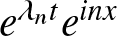 $e^{\lambda_n t} e^{i n x}$, where
 $n$ is an integer, and
 \begin{equation}
\lambda_n = \pm n \sqrt{2 \nu |a|^2-n^2}.
\end{equation}
Therefore, growing modes are possible whenever
 \begin{equation}
0 \lt n^2 \lt 2\nu |a|^2.
\end{equation}
For the remainder of this paper,  $a$ will have the value
 $1$, which leads to the following summary:
 \begin{equation*}
\begin{array}{cl}
0 \lt \nu \lt \frac12 & \text{no unstable modes}\\[3pt]
\frac12 \lt \nu \lt 2 & \text{one unstable mode} \\[3pt]
2 \lt \nu \lt \frac92 & \text{two unstable modes} \\[3pt]
\frac92 \lt \nu \lt 8 & \text{three unstable modes, etc.} \\
\end{array}
\end{equation*}
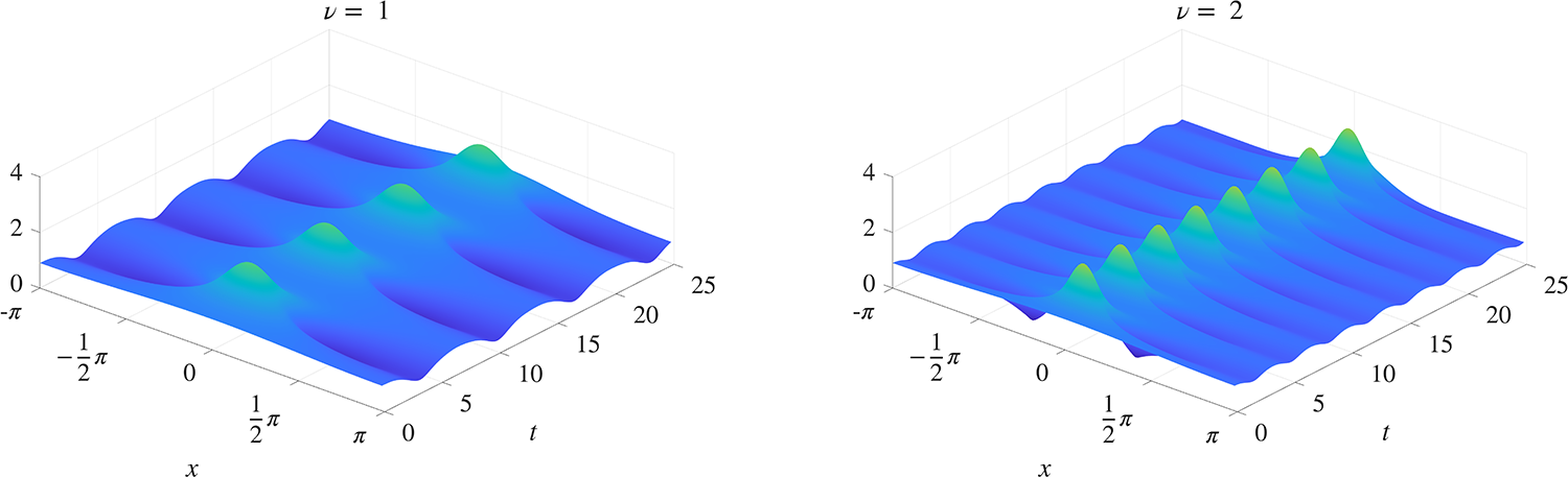
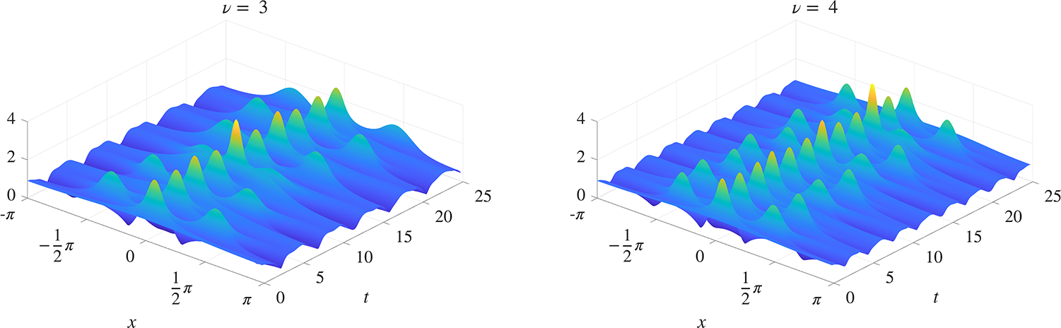
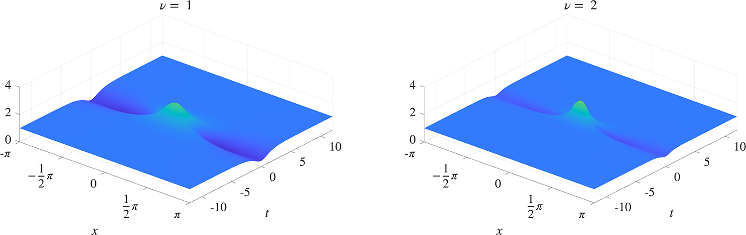
The sequence of solutions shown in Figures 1 and 2 corresponds to 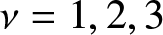 $\nu = 1, 2, 3$ and
 $4$, with the initial condition
 \begin{equation}
u(x,0) = 1 + \epsilon \cos x,
\end{equation}
where 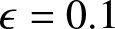 $\epsilon = 0.1$. (This initial condition will be used throughout, with smaller values of
 $\epsilon$ used when comparisons with asymptotic estimates require it.) The case
 $\nu = 1$ represents a single unstable mode, and this shows up as the breather-like solution shown in Figure 1. Initially, the solution grows according to the linear analysis, its modulus forming a single hump corresponding to the single unstable mode. (Remark: Some authors call these humps rogue waves, but here not all of them are sufficiently large to justify that term.) Then nonlinear effects take over and cause it to subside again, after which it returns to the almost uniform initial condition. This is related to the recurrence phenomenon first observed in the Fermi–Pasta–Ulam experiment [Reference Fermi, Pasta and Ulam16]. This behaviour is then repeated periodically in time. When
 $\nu$ increases to values
 $3$ and
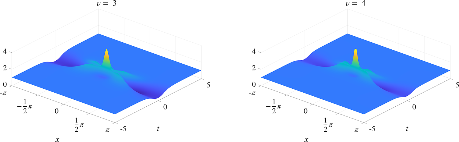
 $4$, an additional mode becomes unstable. This shows up as single- and double-hump profiles taking turns to dominate the solution. A notable difference between these solutions is the fact that the periodic behaviour of Figure 1 is not observed when two unstable modes are present; see Figure 2.
Modulational stability as the value of the nonlinear parameter  $\nu$ is increased. The modulus of the solution of (1.1) is shown over the domain
 $-\pi \leq x \leq \pi, 0 \leq t \leq 25$. The initial condition is (1.6) with
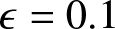 $\epsilon = 0.1$. With
 $\nu = 1$ there is one unstable mode, which grows and subsides periodically. The case
 $\nu = 2$ represents the situation when the second mode is on the edge of instability.

1 Long description
The image consists of two 3D surface plots. The first plot on the left is labeled with a nonlinear parameter value of 1. The x-axis is labeled x, ranging from negative pi over 2 to pi over 2. The t-axis is labeled t, ranging from 0 to 25. The vertical axis represents the modulus of the solution, ranging from 0 to 4. The surface shows periodic waves with peaks around 4. The second plot on the right is labeled with a nonlinear parameter value of 2. The axes are similarly labeled and scaled as the first plot. The surface also shows periodic waves, with more pronounced peaks compared to the first plot, indicating increased instability.
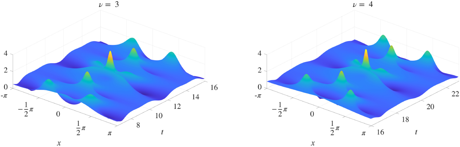
Continuation of Fig. 1. For  $\nu = 3$ and
 $\nu = 4$ there exist two unstable modes, which take turns dominating the solution. No periodicity in time can be discerned.

Figure 2 Long description
Nu equals 3 and nu equals 4. Shared axes for both 3D surface plots: The horizontal axis is labeled, t, ranging from 0 to 25 with ticks at 0, 5, 10, 15, 20, 25. Units are not indicated. The depth axis is labeled, x, ranging from minus pi to pi with ticks at minus pi, minus pi over 2, 0, pi over 2, pi. Units are not indicated. The vertical axis label is not readable. The vertical axis has tick labels 0, 2, 4. Units are not indicated. Plot for nu equals 3: The surface forms repeating ridge-like bands across t. Several taller spikes rise above the ridges around t between 10 and 15. The tallest visible spikes reach close to the tick value 4. Plot for nu equals 4: The surface also forms repeating ridge-like bands across t. Several taller spikes rise above the ridges around t between 10 and 15. The tallest visible spikes reach close to the tick value 4. The ridge pattern and spike region appear similar to the plot for nu equals 3, with no clearly readable numeric difference in peak height from the shown tick marks.
In [Reference Weideman30], the growth and decay of the unstable modes were linked to the dynamics of the poles of the solution in the complex plane. (Remark: singularities of NLS solutions are simple poles, which makes them easier to compute numerically than KdV poles, which are of double multiplicity [Reference Weideman30].) Specifically, if there is a single unstable mode, there are two simple poles that travel as a pair on the imaginary axis, one in the upper half plane and a symmetric partner in the lower half plane. As they travel towards the real axis, the hump steepens, and as they move away, the hump flattens. (Links to animations can be found in the caption of Figure 5.) When there is more than one unstable mode, the pole interaction is more complex, as will be investigated in Section 3. The experiments of [Reference Weideman30] were preliminary, and the present work aims to extend those results.
Pole dynamics of the NLS and the connection to rogue waves have been studied in [Reference Ankiewicz, Clarkson and Akhmediev2, Reference Chiu, Liu, Chan and Chow10, Reference Liu, Chiu, Clarkson and Chow21, Reference Yang and Yang31]. In these studies, the  $x$-domain was the real line, where the NLS admits explicit rational solutions. The pole locations were computed from the denominators of these formulas. In contrast, the periodic domain is considered here, and explicit solutions are rare.
The exception is the well-known Akhmediev breather [Reference Akhmediev and Korneev1, Reference Grinevich and Santini18]. When converted to the particular form of the NLS in (1.1), it is given by
 \begin{equation}
u(x,t) = e^{i \nu t}
\frac{(1/\nu-1)\cosh \big( \sqrt {2\,\nu-1} \, t\big) + i \mu \sqrt{2/\nu}\sinh \big( \sqrt {2\,\nu-1} \, t\big) + \mu \cos x}{\cosh \Big( \sqrt {2\,\nu-1} \, t \Big)-\mu \, \cos x},
\end{equation}
where
 \begin{equation}
\mu := \sqrt{\frac{2\nu-1}{2\nu}}, \quad \nu \geq \frac12.
\end{equation}
This solution is shown in Figure 3, for the cases  $\nu = 1$ and
 $\nu = 2$. Unlike the solutions shown in Figure 1, these solutions are not periodic in time. However, with appropriate translation, each of the hump-like structures in the solutions of Figure 1 can be approximated locally by the corresponding Akhmediev breather in the small
 $\epsilon$ limit [Reference Grinevich and Santini18]. Numerical verification of this will be given in Section 2. (Remark: The formula (1.7) is not the most general form of the Akhmediev breather: shifts in time and space can be included as well as a constant phase factor.)
Two examples of the Akhmediev breather. The modulus of the solution (1.7) is shown.

Figure 3 Long description
Two examples of the Akhmediev breather. The modulus of the solution is shown. The image A showing a 3D surface plot for mu equals 1, representing the modulus of the solution over time and space. The x-axis is labeled t, ranging from minus 10 to 10 and the y-axis is labeled x, ranging from minus 2 pi to 2 pi. The z-axis represents the modulus of the solution, with tick labels at 0, 2 and 4. The surface has a central peak around t equals 0 and x equals 0, with a height close to 3. The peak is narrow and the surface decreases outward. The image B showing a 3D surface plot for mu equals 2, with similar axes and ranges. The central peak is slightly higher, around 3.5 and wider compared to mu equals 1. The modulus of the solution is plotted, illustrating how the parameter mu affects the amplitude and spread of the solution. The plots demonstrate the behavior of the Akhmediev breather solution over time and space, with mu controlling the solution′s characteristics. The comparison shows that increasing mu results in a higher and wider peak, affecting the solution′s spread across the surface.
2. One unstable mode
Before looking at pole dynamics, first consider the maximum height reached by the humps in Figure 1. For this, define the growth factor as
 \begin{equation}
\gamma(\nu) = \frac{\displaystyle \max_{-\pi \leq x \leq \pi \atop t \gt 0 }|u(x,t)|}{\displaystyle \max_{-\pi \leq x \leq \pi}|u(x,0)|}.
\end{equation}
For the initial condition (1.6), the denominator in this expression is 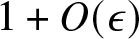 $1+O(\epsilon)$. By the asymptotic estimates of [Reference Grinevich and Santini18], the numerator can be estimated to
 $O(\epsilon)$ by evaluating the Akhmediev breather (1.7) at
 $(x,t) = (0,0)$, which gives
 \begin{equation}
\gamma(\nu) = \frac{1/\nu-1+\mu}{1-\mu}
\end{equation}
to first order in  $\epsilon$. This evaluates to
 $\gamma(1) = 1+\sqrt{2}$ and
 $\gamma(2) = 1+\sqrt{3}$; the latter value is also recorded in [Reference Grinevich and Santini18]. Two other special cases are of interest: Firstly, solving
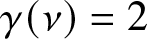 $\gamma(\nu) = 2$ gives
 $\nu = \frac23$; this is significant because the rogue wave threshold is often defined to be a height of twice the unperturbed surface (namely
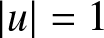 $|u| = 1$ in this case). Secondly,
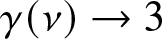 $\gamma(\nu) \to 3$ as
 $\nu \to \infty$. In Section 3, it will be shown that the Akhmediev breather remains relevant for values of
 $\nu$ also larger than
 $2$, and this shows that the generic growth is bounded by a factor
 $3$. There exist anomalous cases, however, where the factor can be much larger than
 $3$, as will be explored in the next two sections.
Other values of  $\nu$ in the interval
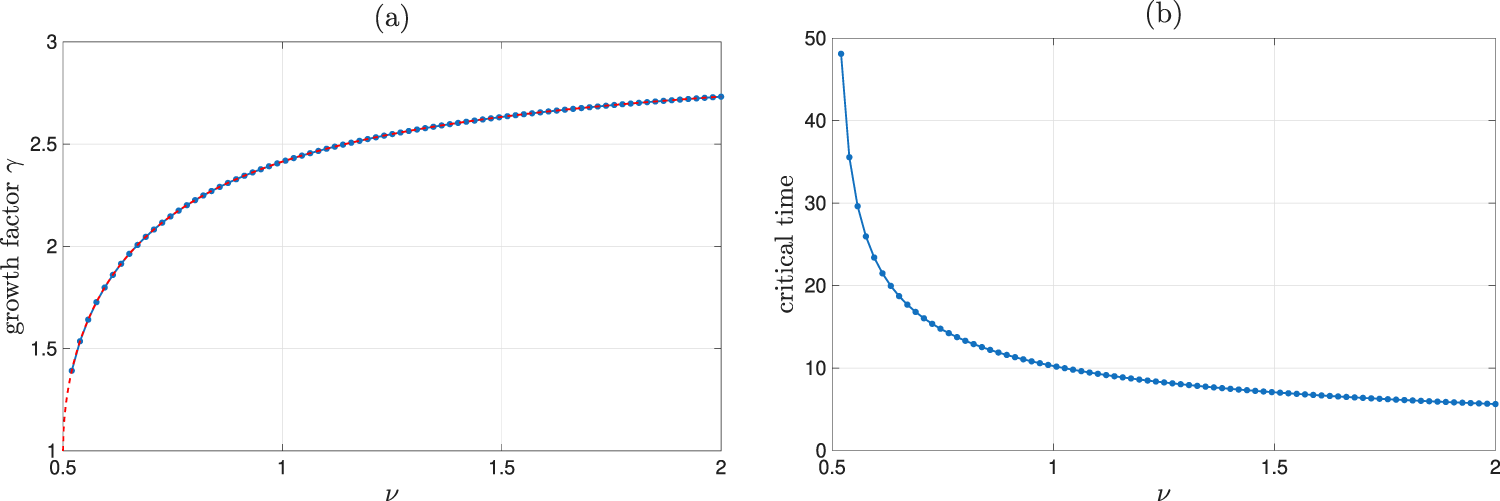
 $(\frac12,2)$ are represented in the graph of Figure 4(a). The good agreement between the estimate (2.2) and the numerically computed values serves as verification of the theorem of [Reference Grinevich and Santini18]. (The asymptotic limit in that theorem is
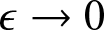 $\epsilon \to 0$. To make the verification more convincing, the value of
 $\epsilon$ was therefore reduced from
 $10^{-1}$ used elsewhere to
 $10^{-4}$ in Figure 4.) Also shown in frame (b) of that figure is the numerical approximation of the smallest value of
 $t$ where the maximum in (2.2) is achieved, i.e., the critical time when the first hump reaches maximum height. The fact that the humps occur with a period inversely proportional to
 $\nu$, consistent with the two-mode analysis of [Reference Infeld19, Reference Weideman and Herbst28], is also clear from Figure 4(b).
(a) The growth factor  $\gamma(\nu)$, defined by (2.1). The blue dots were computed by solving the NLS (1.1) numerically, and the red dotted curve (hardly visible) is the asymptotic estimate (2.2). (b) The critical value of
 $t$ when the first hump reaches its maximum. In both figures, the initial condition is (1.6), with
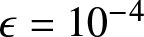 $\epsilon = 10^{-4}$.

Turning to pole dynamics, in the case of a single unstable mode, the motion of the poles is straightforward. Because the initial condition (1.6) has no singularities in the finite complex plane, a pair of poles is born at infinity and then travels along the imaginary axis, symmetrically with respect to the real axis. They approach the real axis but at a critical time reverse their direction; this is the time when the humps in Figure 1 reach their maximum growth. They then move back along the imaginary axis out to infinity, this being the time of recurrence. The process then repeats periodically. Links to animations for the cases  $\nu = 1$ and
 $\nu = 2$ are given in Figure 5. (It might be of interest to note that this pole behaviour is similar to that of the viscous Burgers equation analysed in [Reference Senouf23, Reference Senouf24] and computed in [Reference Weideman30]. In that case, a string of poles – not just one pair as in the case of the NLS – travels along the imaginary axis, and causes a near-shock when the front-running pair reaches a minimum distance to the real axis. Following that, they recede to infinity as steady-state is approached.)
The location of the pole at its closest point to the real axis can also be estimated from the theory of [Reference Grinevich and Santini18]. The substitution of  $t = 0$ into the denominator of (1.7) shows that these locations are on the imaginary axis, at
 $\pm iy$, where
 \begin{equation}
y = \mbox{arccosh}(1/\mu).
\end{equation}
The numerical confirmation of this is given in Figure 5.
Numerically computed pole locations on the positive imaginary axis as a function of  $t$, for the two solutions shown in Fig. 1 (where
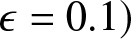 $\epsilon = 0.1)$. The asymptotic estimate of the pole location closest to the real axis is given by (2.3). For the cases
 $\nu=1$ and
 $\nu=2$, that expression evaluates to
 $0.88$ and
 $0.55$, respectively, which agrees well with the numerical results shown. Animations: Nu1.mp4, Nu2.mp4.

3. More than one unstable mode
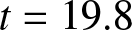
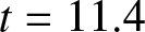
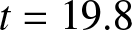
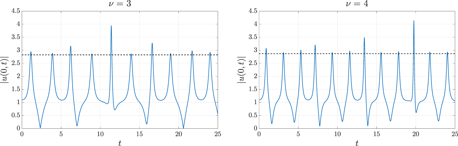
When there is more than one unstable mode, the evolution is more complex: compare Figures 1 and 2. Not only is the evolution not periodic in time, but the peaks reach different heights, with some peaks significantly higher than others. For example, such anomalous peaks can be seen in Figure 2, roughly at time 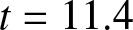 $t = 11.4$ when
 $\nu = 3$, and at
 $t = 19.8$ when
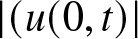
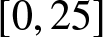
 $\nu = 4$. A clearer picture is shown in Figure 6, which shows the evolution of
 $|(u(0,t)|$, for
 $t$ in
 $[0,25]$. There, the heights of the peaks are compared to the height of the corresponding Akhmediev breather (2.2), taken to be the reference height for the generic peaks. The anomalous peaks grow to about four times the height of the unperturbed solution level
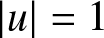 $|u|=1$, while that factor is only about three times for generic waves.
The evolution of 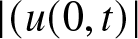 $|(u(0,t)|$, shown as the continuous curves, for the two solutions shown in Fig. 2. The dotted horizontal lines are the reference heights defined by the Akhmediev breather (2.2). Most peaks are at around this height, but roughly at
 $t = 11.4$ (
 $\nu = 3$) and at
 $t = 19.8$ (
 $\nu = 4$), there are anomalous peaks that are substantially higher than the reference value.

Figure 7 shows the same solutions as in Figure 2, but now zoomed in on the two anomalous peaks identified in Figure 6. In the generic case, the two unstable modes take turns to dominate the solution. The anomalous situation occurs when they dominate the solution at the same time. This has been referred to as the ‘coalescing of modes’ and has been suggested as a possible mechanism for the creation of rogue waves in [Reference Calini and Schober9].
Same as Fig. 2, but restricted to a smaller time interval that includes the anomalous peaks identified in Fig. 6. The extra height occurs when the two unstable modes reach their turn to dominate at the same time.

Figure 7 Long description
Two three dimensional surface plots compare p equals 3 and p equals 4, showing surface height over x and r. The x-axis is labeled x with tick labels minus 1, 0, 1 and 2. The r-axis has tick labels 8, 10, 12, 14, 16, 18, 20 and 22. The vertical axis represents surface height, but the label and units are not shown. For p equals 3, peaks are concentrated around r values 10 to 16, with the tallest peak exceeding the 4 tick mark near x equals 1. For p equals 4, peaks shift to higher r values, around 12 to 20, with the tallest peak also exceeding the 4 tick mark near x equals 1. The plots illustrate how increasing p shifts peak locations to higher r values while maintaining similar peak heights.
There exists a two-mode extension of the Akhmediev breather (1.7), which could be related to the anomalous peaks shown in Figure 7. Two of these breathers, when scaled to the interval 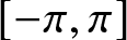 $[-\pi,\pi]$, are shown in Figure 8. (Remark: The formulas for these 2-breathers are cumbersome and not given here; they can be found in [Reference Calini and Schober9, eq. (13)–(16)] and [Reference Grinevich and Santini18, eqs. (24)–(27)].) There is qualitative agreement between Figures 7 and 8, but making the correspondence quantitative is not simple due to the number of free parameters in the formula for the two-mode breather. The examples in Figure 8 were constructed by experimenting with those parameters until a reasonable visual match was found. Similar solutions are shown in [Reference Calini and Schober9, Fig. 2] and [Reference Chiu, Liu, Chan and Chow10, Fig. 3].
Two examples of Akhmediev 2-breathers. These are in qualitative agreement with the anomalous peaks shown in Fig. 7.

The pole dynamics in the cases where there is more than one unstable mode are a lot more complex than the simple periodic motion of a single pair of poles along the imaginary axis as discussed in Section 2. The primary poles on the imaginary axis persist, driving the growth and decay of the fundamental mode. But they are now joined by secondary pairs of poles located off the imaginary axis, symmetric with respect to that axis (a consequence of the symmetry of the equation and the initial condition (1.6)).
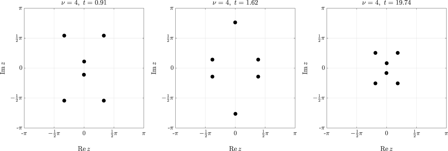
Some pole configurations for  $\nu = 4$ are shown in Figure 9. (These are qualitatively similar to the configurations for
 $\nu = 3$.) The first frame shows a situation where the primary pair of poles reaches a minimum distance from the real axis, and the second frame shows the same for the secondary poles. The anomalous situation, where both fundamental and secondary poles are close to the origin, is shown in the third frame. In between these critical times, the secondary poles trace complicated trajectories in the complex plane. At certain times, they approach the real axis, but then loop around, back out to infinity in the imaginary direction. At other times, they approach the origin, but are then repelled by the primary poles. None of the poles seems to leave the strip
 $-\frac12 \pi \lt \mbox{Re} \, z \lt \frac12 \pi$ at any time. Links to animations of this behaviour can be found in the caption of Figure 9.
Pole configurations at critical times in the case  $\nu = 4$; compare Fig. 2. The first frame corresponds to the first instance the single-hump reaches its peak, and the second frame to the first time the double-humps do so. The third frame corresponds to the anomalous situation identified in Fig. 6, where the two unstable modes seem to coalesce. Animations: Nu3.mp4, Nu4.mp4.

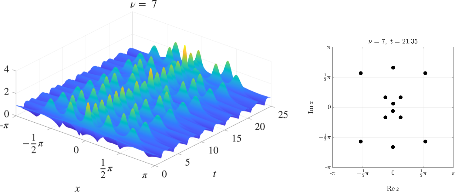
The last example, presented in Figure 10, is a case where there are three unstable modes. On the left, an anomalous peak can be seen at approximately  $t = 21.35$. The corresponding pole configuration, shown on the right, is remarkably similar to the configuration shown in [Reference Ankiewicz, Clarkson and Akhmediev2, Fig. 1] (which was computed from an explicit rational solution). This suggests that these anomalous pole configurations might be a generic feature of the NLS.
An example with three unstable modes. On the left, the modulus of the solution for  $\nu = 7$ is shown, revealing an anomalous peak near
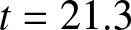 $t = 21.3$. The corresponding pole configuration at that instant is shown on the right. Now six pairs of poles seem to coalesce at the critical time. Animation: Nu7.mp4.

Figure 10 Long description
A showing a 3D surface plot with the title text, nu equals 7. The horizontal axis along the front edge is labeled x, with tick labels minus pi, minus 1 over 2 pi, 0, 1 over 2 pi and pi. The horizontal axis along the right edge is labeled t, with tick labels 0, 5, 10, 15, 20 and 25. The vertical axis has tick labels 0, 2 and 4. The surface shows repeating ridges along t and multiple narrow spikes, with the tallest spikes located around t between about 15 and 22 and x near 0 to 1 over 2 pi. B showing a scatter plot with the title text, nu equals 7, t equals 21.35. The horizontal axis is labeled Re z, with tick labels minus pi, minus 1 over 2 pi, 0, 1 over 2 pi and pi. The vertical axis is labeled Im z, with tick labels minus pi, minus 1 over 2 pi, 0, 1 over 2 pi and pi. There are 12 plotted points. Four points lie near the corners at approximately Re z equals minus 1 over 2 pi and Im z equals 1 over 2 pi, Re z equals 1 over 2 pi and Im z equals 1 over 2 pi, Re z equals minus 1 over 2 pi and Im z equals minus 1 over 2 pi and Re z equals 1 over 2 pi and Im z equals minus 1 over 2 pi. One point lies on the vertical axis near Im z equals minus 1 over 2 pi. One point lies on the vertical axis near Im z equals 1 over 2 pi. The remaining six points form a cluster around the origin, with points on or near Re z equals 0 and Im z equals 0 and additional points slightly offset to the left, right, above and below the origin.
4. Conclusion
Modulational instability in the NLS is a well-studied field, with a variety of analytical tools that can be brought to bear on the problem. In contrast, the present study utilised numerical methods, specifically to track the motion of the poles that drive the instability. This work was started in [Reference Weideman30], a review paper that focused more on the Burgers and KdV equations, with NLS results limited to a single figure. The subsequent explorations reported here focused on establishing the trajectories of the NLS poles.
It was found that the pole dynamics ranged from simple periodic motion along the imaginary axis to quite complicated trajectories in the complex plane. Pole configurations associated with maximal instability were identified, which may be of interest to rogue wave investigations. As part of the investigation, an asymptotic estimate found in the literature was numerically verified.
The hope is that this view from the complex plane may stimulate further analysis that would lead to a better understanding of modulational instability as it occurs in various applications.
Supplementary material
The supplementary material for this article can be found at https://doi.org/10.1017/jnw.2026.10044.
Data availability statement
No data were used.
Acknowledgements
This work was presented at the 80th birthday celebrations of Mark Ablowitz in June 2025 in Boulder, Colorado. Much appreciation goes to Mark, who was always welcoming and supportive during numerous visits to Boulder over the years. The author is also grateful to the organisers for the invitation to speak at the meeting. Discussions with Ben Herbst are also acknowledged, as is the input from anonymous referees.
Author contributions
Single-authored paper.
Funding statement
No funding was received for this research.
Competing interests
None.
Ethical standards
Not applicable.
Appendix A. Numerical Pole Tracking
The pole tracking used in this paper is done in two phases. In the first, the equation is solved on the real line using a Fourier method combined with an accurate time integrator. In the second, the solution is continued into the complex plane using the Fourier–Padé method [Reference Driscoll and Fornberg12, Reference Weideman30].
The recommended candidate for the first phase is the Fourier pseudospectral method, which leads to a semi-discrete version of the NLS
 \begin{equation}
\frac{d u_j}{dt} = i D_2 u_j + i \nu |u_j|^2 u_j, \qquad j = -N, \ldots, N-1.
\end{equation}
The  $u_j$ represent the approximations to
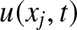 $u(x_j,t)$ on the grid
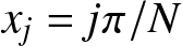 $x_j = j\pi/N$. The
 $D_2$ is the Fourier second derivative operator (which converts the function values to Fourier space, differentiates there and returns to physical space, with both the forward and inverse transforms done with FFTs). For the time integration, split-step methods and exponential integrators are popular [Reference Berland, Islas and Schober5], but current versions do not allow for error control. For the high accuracy required here, MATLAB’s ode15s function was used instead. It implements both variable order and variable step-sizes for error control (tolerances were set to
 $10^{-10}$). In addition, being based on backward differentiation formulas, ode15s is suitable for the stiffness in the system associated with the second derivative operator [Reference Shampine and Reichelt25].
After solving the system (A.1), an FFT can be used at each time step to convert function values to Fourier coefficients, which then yields the approximation
 \begin{equation}
u(x,t) \approx \sum_{k=-N}^{N} c_k(t) e^{ik x}, \quad -\pi \leq x \lt \pi.
\end{equation}
Because it is an entire function, this series will reveal very little about the pole locations in the complex plane. To obtain such information, one strategy is to convert this into a rational trigonometric form where pole information can be extracted from the denominator. The first step is to discard all terms in (A.2) without information content. For example, if  $N$ is sufficiently large, then the values of the
 $|c_k|$ will plateau at roundoff level for
 $k$ large enough. Here, all trailing terms with
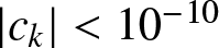 $|c_k| \lt 10^{-10}$ were set to zero, leading to a truncated version of (A.2) with
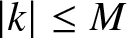 $|k| \leq M$. (The values of
 $c_k$ and
 $M$ depend on
 $t$, but this dependence will be suppressed in what follows.)
By setting 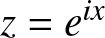 $z = e^{ix}$ and splitting the truncated series (A.2) into terms with
 $k \gt 0$ and
 $k \lt 0$ one gets
 \begin{equation}
\sum_{k=-M}^{M} c_k e^{ik x} = f_-(z) + f_+(z),
\end{equation}
where
 \begin{equation}
f_+(z) = \frac12 c_0 + \sum_{k=1}^M c_k z^k,
\end{equation}
with a similar expression for  $f_-(z)$. The polynomial (A.4) can be converted to a rational function, say
 $r_+(z)$, by the method of Padé approximation [Reference Baker and Graves-Morris3]. (This involves writing
 $r_+(z) = p_+(z)/q_+(z)$ where both numerator and denominator polynomials are assumed here to have degree
 $\frac12 M$, with
 $M$ even. Clearing the denominator and requiring that the resulting polynomial equation is satisfied to maximal degree, a linear system is obtained that can be solved for the coefficients of
 $p_+(z)$ and
 $q_+(z)$.) Doing the same for
 $f_-(z)$, one obtains the Fourier–Padé approximation
 \begin{equation}
u(x,t) \approx r_-(e^{-ix}) + r_+(e^{ix}).
\end{equation}
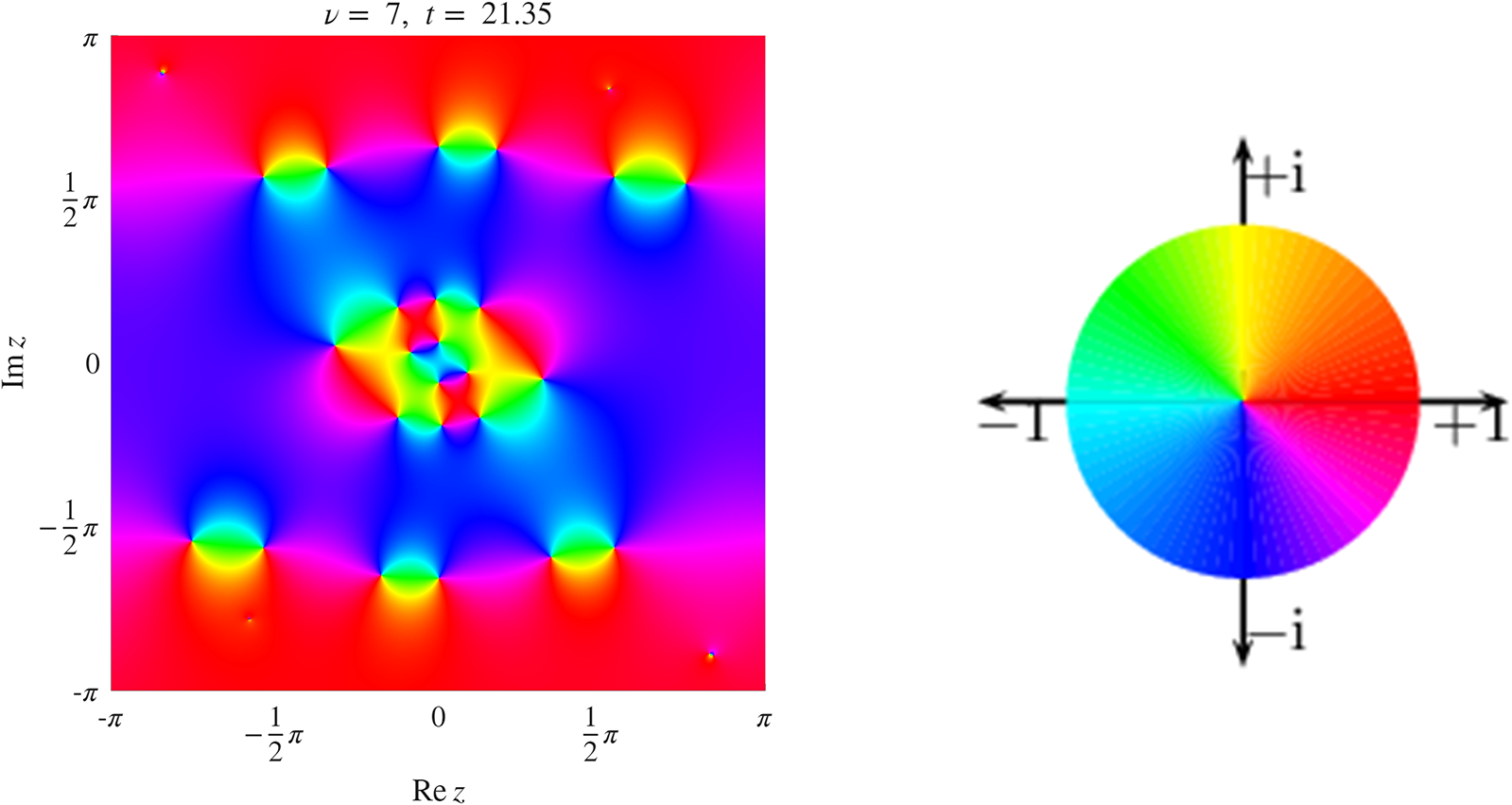
Pole locations can be computed by applying a root-finding algorithm to the denominator of (A.5). For visual representation, as shown in Figures 9 and 10, for example, high accuracy is not required. There, and in the animations of Figures 5, 9 and 10, poles have been located by evaluating (A.5) on a fine grid in the complex plane and searching for local maxima of  $|u|$ (using MATLAB’s function islocalmax2). Another method is to represent (A.5) as a phase plot, shown in Figure A1 (see also [Reference Weideman30]). It provides phase information in addition to pole locations, but in animations it makes the pole motion harder to follow visually.
Phase plot representation of the pole configuration in Fig. 10 (produced by the software of [Reference Wegert27]). The colour wheel is shown on the right: Real and positive values (resp. negative) are shown as red (resp. cyan). Likewise, pure imaginary values are shown as yellow or dark blue, etc. Poles and zeros are located at the critical points where the colours meet. Poles (resp. zeros) are identified by the colours running in a clockwise direction (resp. anti-clockwise). The fact that the colour wheel is traversed only once at each of these critical points confirms that the poles (as well as the zeros) are simple.

Figure A1 Long description
The composite figure contains two parts: a square phase map of a complex function plotted over the complex plane and a separate circular phase wheel used as a legend for interpreting the phase values shown in the map. The phase map has a horizontal axis labeled Re z, ranging from minus pi to pi, with tick marks at minus pi, minus 1 over 2 pi, 0, 1 over 2 pi and pi. The vertical axis is labeled Im z, ranging from minus pi to pi, with the same tick increments. A label above the plot reads nu equals 7, l equals 21.35, where nu equals 7 identifies the mode number and l equals 21.35 identifies the associated parameter value. The plot displays a continuous phase field across the entire complex plane domain. Multiple singular points are visible where distinct phase regions converge. A cluster of singular points appears at and near the origin, at approximately 0 and 0. Additional singular points are distributed symmetrically at locations near the boundaries of the domain, appearing at positions close to plus or minus pi along both the real and imaginary axes. The arrangement of these singular points follows a symmetric pattern about both the real and imaginary axes. The phase wheel legend is a circle with four directional arrows extending outward along the cardinal directions. The rightward arrow is labeled plus 1, corresponding to positive real values. The leftward arrow is labeled minus 1, corresponding to negative real values. The upward arrow is labeled plus i, corresponding to positive imaginary values. The downward arrow is labeled minus i, corresponding to negative imaginary values. The wheel maps phase angle continuously around the full 360 degrees, allowing identification of zeros and poles at points where phase regions meet in the main plot.
Among computational mathematicians, numerical analytic continuation is known not as a science but as an art. In the absence of theoretical proofs, one has to rely on plausibility checks to gain confidence in the results. For example, by representing the solution as a phase plot (see Figure A1) one can check that the poles have the right order. Residues can be checked by numerical contour integration. Spurious poles (a well-known artefact in Padé methods) can be identified by symmetry breaking or by their appearance and disappearance from one time step to the next.
Moreover, there are limits on how far one can push into the upper and lower half-planes; the further out, the more unstable the process. (For example, spurious poles with tiny residues can be seen near the four corners of Figure A1.) Also, in the case of the NLS, the smaller the value of  $\epsilon$ in the initial condition (1.6), the more unreliable the pole tracking becomes. (Presumably, this is caused by the proximity to the unstable homoclinic orbit [Reference Calini and Schober9].) Likewise, larger values of
 $\nu$ imply more unstable modes, which poses an increasingly difficult challenge. The case of three unstable modes, shown in Fig. 10, seems to be the limit in standard floating-point arithmetic. In both the small
 $\epsilon$ and the large
 $\nu$ cases, a switch to quadruple precision might help, but this has not been explored yet.
















 Open access

