1 Introduction
High viscosity liquids such as polymer melts, foods, paints, pharmaceutics and cosmetics are usually processed in rotary equipment which can generate shear, extensional, but in general, much more complicated flows. When a drop is present in these types of flows it will deform, and if the strength of the flow exceeds some critical value, the drop may even break. The deformation of the drop spans a wide domain, from a slightly perturbed sphere up to a slender body with pointed ends. This phenomenon of deformation and breakup of drops in viscous liquids can be found in many physical problems, such as in the design of efficient emulsifiers and homogenizers. While most of the creeping flow literature refers to small and medium deformations, this report is dedicated to slender drops only. The reviews of Rallison (Reference Rallison1984), Stone (Reference Stone1994), and Briscoe, Lawrence & Mietus (Reference Briscoe, Lawrence and Mietus1999) and the books of Clift, Grace & Weber (Reference Clift, Grace and Weber1978), Levitskiy & Shulman (Reference Levitskiy and Shulman1995), Sadhal, Ayyaswamy & Chung (Reference Sadhal, Ayyaswamy and Chung1997), Zapryanov & Tabakova (Reference Zapryanov and Tabakova1999) and Chhabra (Reference Chhabra2006), contain an extensive literature review and discuss many industrial applications of this subject.
Slender drops were experimentally observed many years ago by Taylor (Reference Taylor1934). Such drops were produced in a parallel-band apparatus (simple shear flow) and in a four-roller apparatus (two-dimensional extensional flow). Thirty years later, Taylor (Reference Taylor1964) suggested a theoretical treatment for the deformation and breakup of a slender drop in an axisymmetric linear extensional creeping flow, a case where the cross-section of the drop is circular. The theory, that was refined by Buckmaster (Reference Buckmaster1972, Reference Buckmaster1973), Acrivos & Lo (Reference Acrivos and Lo1978) and others, suggests a drop with a parabolic radius profile having pointed ends. The problem is governed by two dimensionless parameters: the large capillary number
 $Ca=\unicode[STIX]{x1D707}Aa/\unicode[STIX]{x1D70E}\gg 1$
and the small viscosity ratio
 $\unicode[STIX]{x1D706}=\unicode[STIX]{x1D707}_{in}/\unicode[STIX]{x1D707}\ll 1$
. Here
 $a$
is the equivalent radius (the radius of a sphere having the same volume as the deformed drop),
 $A$
is the extension rate,
 $\unicode[STIX]{x1D707}$
and
 $\unicode[STIX]{x1D707}_{in}$
are the viscosities of the external and internal fluids, respectively, and
 $\unicode[STIX]{x1D70E}$
is the surface tension. A further exploration reveals that the number of dimensionless governing parameters can be reduced from two
 $(Ca,\unicode[STIX]{x1D706})$
to one: the viscous strength of the flow
 $F=Ca\unicode[STIX]{x1D706}^{1/6}\sim O(1)$
. As
 $F$
increases, the drop becomes thinner and longer until the breakup point at
 $F=0.148.$
It follows that a bubble or an inviscid drop
 $(F=0)$
in a linear extensional creeping flow is always stable and breakup is not possible.
Over the years, a few theoretical extensions have been suggested. A slender drop in a two-dimensional extensional flow was treated by Hinch & Acrivos (Reference Hinch and Acrivos1979), since it describes better (than the axisymmetric case) the experiments performed in a four-roller apparatus. Although the cross-section was found to be significantly non-circular, the breakup criterion was practically identical to the axisymmetric case. Acrivos & Lo (Reference Acrivos and Lo1978) suggested including weak inertial effects
 $(Re\ll 1)$
to the external fluid as the Reynolds number based on the length of a long slender drop may be not so small. The analysis, that was expanded by Favelukis, Lavrenteva & Nir (Reference Favelukis, Lavrenteva and Nir2006), predicts that contrary to the creeping flow case, an inviscid drop
 $(F=0)$
can be broken. As inertia increases, drop breakup is facilitated as it requires less critical values of
 $F$
. The evolution studies of Favelukis, Lavrenteva & Nir (Reference Favelukis, Lavrenteva and Nir2012), show that under creeping flow conditions or at low inertia intensity the drop breaks up via indefinite elongation, while for an inviscid drop or at higher inertia intensities the drop breaks via a centre pinching mechanism. Brady & Acrivos (Reference Brady and Acrivos1982) considered the effects of inertia inside and outside the drop and found that internal inertia has a weak effect on drop breakup. A slender non-axisymmetric drop was treated by Howell & Siegel (Reference Howell and Siegel2004), while Booty & Siegel (Reference Booty and Siegel2005) investigated an insoluble surfactant on the surface of an inviscid slender drop.
Sherwood (Reference Sherwood1984) included nonlinear terms to the extensional creeping flow as it describes better (than the linear flow) the outer flow in Taylor’s four-roller apparatus, see also Antanovskii (Reference Antanovskii1996). The theory that was recently reviewed and expanded by Favelukis (Reference Favelukis2016) suggests a problem which is governed by two
 $O(1)$
dimensionless parameters. The viscous strength of the flow
 $F=Ca\unicode[STIX]{x1D706}^{1/6}$
and the nonlinear strength of the flow
 $G=Ca^{4}E$
, where
 $E=Ba^{2}/A$
such that
 $|E|\ll 1$
, and
 $B$
is connected to the nonlinearity of the velocity. Similar to linear extensional flow
 $(G=0)$
, nonlinear effects
 $(G\neq 0)$
do not change the shape at the end of the steady drop which is still pointed. Contrary to the linear flow, where a bubble or an inviscid drop
 $(F=0)$
cannot be broken, the nonlinear flow can cause a bubble to break. In the linear extensional flow, the local radius of the drop decreases monotonically
 $(z\geqslant 0)$
while in the nonlinear flow, the local radius may decrease monotonically (stable or unstable) or may have a local maximum, besides the one at the centre of the drop (unstable). Three types of breakup mechanisms were discovered, a centre pinching mode, indefinite elongation and mechanism reminding us of tip-streaming where a cusp is developed at the end of the drop.
So far, our discussion has been limited to slender drops in Newtonian systems. The only theoretical studies in extensional flow dealing specifically with slender drops in non-Newtonian systems are our previous reports which include non-Newtonian behaviour inside (Favelukis, Lavrenteva & Nir Reference Favelukis, Lavrenteva and Nir2005; Favelukis et al.
Reference Favelukis, Lavrenteva and Nir2006), and outside the drop (Favelukis & Nir Reference Favelukis and Nir2001). For the case of a power-law non-Newtonian slender drop in a linear extensional creeping flow, the problem is governed by the viscous strength of flow
 $F=Ca\unicode[STIX]{x1D706}^{1/[3(1+n)]}$
and the power-law index
 $n$
. Only shear thinning and Newtonian drops
 $(n\leqslant 1)$
with pointed ends exist, with (for the same
 $F$
) Newtonian drops being more elongated than shear thinning drops. For the same viscosity ratio, shear thinning drops are more difficult to break than Newtonian drops, as they require higher critical capillary numbers. A few experiments with non-Newtonian drops experiencing medium deformations were performed. In the entrance region to a tube (Han & Funatsu Reference Han and Funatsu1978), in planar extensional flow (Milliken & Leal Reference Milliken and Leal1991; Tretheway & Leal Reference Tretheway and Leal1999) or in uniaxial elongational flows (Delaby et al.
Reference Delaby, Ernst, Germain and Muller1994). No experimental study primarily focuses on non-Newtonian slender drops; yet, extrapolation of medium deformation findings indicate that non-Newtonian drops are less deformable than Newtonian ones as predicted by the theory.
Two of the extensions concerning slender drops in an extensional creeping flow that were discussed above are (i) a Newtonian drop in a nonlinear extensional flow (Favelukis Reference Favelukis2016), as it describes better (than the linear flow) the flow occurring in industrial rotating equipment; and (ii) a non-Newtonian drop in a linear extensional flow (Favelukis et al.
Reference Favelukis, Lavrenteva and Nir2005, Reference Favelukis, Lavrenteva and Nir2006), as it describes better (than the Newtonian drop) the behaviour of polymer liquids. These cases resulted in interesting findings and their combination, a non-Newtonian slender drop in a nonlinear extensional flow, is the subject of this report. Similar to previous cases, we shall see that only Newtonian and shear thinning drops
 $(n\leqslant 1)$
with pointed ends are possible, with shear thinning drops being less elongated and more difficult to break than Newtonian drops. Furthermore, we shall also conclude that as the flow becomes more nonlinear, drop breakup is facilitated.
2 The governing equations
2.1 The flow outside the drop
Consider the motion suggested by Sherwood (Reference Sherwood1984) for an incompressible Newtonian fluid undergoing an axisymmetric nonlinear extensional creeping flow. In cylindrical coordinates, the velocity components and the pressure of the undisturbed motion are
 $$\begin{eqnarray}\displaystyle & \displaystyle v_{r}=-{\textstyle \frac{1}{2}}Ar-{\textstyle \frac{3}{2}}Brz^{2}, & \displaystyle\end{eqnarray}$$
 $$\begin{eqnarray}\displaystyle & \displaystyle v_{z}=Az+Bz^{3}, & \displaystyle\end{eqnarray}$$
 $$\begin{eqnarray}\displaystyle & \displaystyle p=3\unicode[STIX]{x1D707}B(z^{2}-{\textstyle \frac{1}{2}}r^{2}). & \displaystyle\end{eqnarray}$$
Note that Sherwood (Reference Sherwood1984) excluded quadratic terms in the velocity in order to maintain the symmetry at
 $z=0$
. We assume that
 $A>0$
, yet we allow
 $B$
to be positive or negative. When
 $B=0$
, the familiar (linear) extensional flow is obtained and
 $A$
becomes the extension rate.
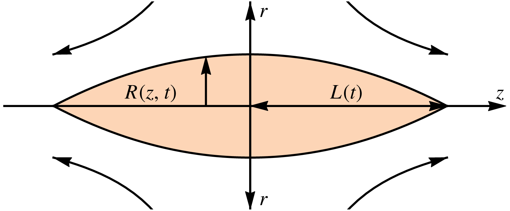
Next, and as described in figure 1, we place a drop at the origin of the coordinate system. Then, under certain conditions described later, a slender drop with a local radius
 $R(z,t)$
and a half-length
 $L(t)$
, such that
 $R/L\ll 1$
, can be obtained.
A slender drop in an axisymmetric extensional creeping flow:
 $R(z,t)$
is the local radius and
 $L(t)$
is the half-length of the drop.

According to Acrivos & Lo (Reference Acrivos and Lo1978), for a slender drop, only the radial component of the velocity is disturbed which can be found from the continuity equation and the kinematic condition. Together with the Stokes equation we find the leading order of the disturbed motion just outside the drop to be (Favelukis Reference Favelukis2016)
 $$\begin{eqnarray}\displaystyle & \displaystyle v_{r}=\frac{R}{r}\frac{\unicode[STIX]{x2202}R}{\unicode[STIX]{x2202}t}+A\left\{-\left(1+3\frac{B}{A}z^{2}\right)\frac{r}{2}+\frac{R}{r}\left[\left(1+3\frac{B}{A}z^{2}\right)\frac{R}{2}+\left(1+\frac{B}{A}z^{2}\right)z\frac{\unicode[STIX]{x2202}R}{\unicode[STIX]{x2202}z}\right]\right\}\qquad & \displaystyle\end{eqnarray}$$
 $$\begin{eqnarray}\displaystyle & \displaystyle v_{z}=Az\left(1+\frac{B}{A}z^{2}\right), & \displaystyle\end{eqnarray}$$
 $$\begin{eqnarray}\displaystyle & \displaystyle p_{out}=3\unicode[STIX]{x1D707}Bz^{2}. & \displaystyle\end{eqnarray}$$
2.2 The flow inside the drop
Let the incompressible non-Newtonian fluid inside the drop be described by the simple power-law model
 $$\begin{eqnarray}\unicode[STIX]{x1D749}=m\left|\sqrt{\frac{1}{2}(\dot{\unicode[STIX]{x1D738}}\boldsymbol{ : }\dot{\unicode[STIX]{x1D738}})}\right|^{n-1}\dot{\unicode[STIX]{x1D738}},\end{eqnarray}$$
with
 $\unicode[STIX]{x1D749}$
being the viscous stress tensor,
 $\dot{\unicode[STIX]{x1D738}}$
is the rate of deformation tensor and
 $m$
and
 $n$
are parameters of the model. In a Newtonian fluid
 $n=1$
and
 $m$
is the Newtonian viscosity. For a shear thinning (pseudoplastic) fluid
 $n<1$
and in a shear thickening (dilatant) fluid
 $n>1$
.
According to Taylor (Reference Taylor1964), the flow inside a slender drop is a Poiseuille flow with an axial velocity at the surface of the drop
 $(r=R)$
, given by (2.2) or (2.5), and a positive pressure gradient
 $(z\geqslant 0)$
. Based on these assumptions and the equation of motion under creeping flow conditions we can develop the internal velocity profile for the region
 $0\leqslant z\leqslant L$
 $$\begin{eqnarray}v_{z}=A\left(1+\frac{B}{A}z^{2}\right)z-\left(\frac{n}{1+n}\right)\left(\frac{R}{2m}\frac{\unicode[STIX]{x2202}p_{in}}{\unicode[STIX]{x2202}z}\right)^{1/n}R\left[1-\left(\frac{r}{R}\right)^{1+1/n}\right],\end{eqnarray}$$
where
 $p_{in}$
is the pressure inside the drop, assumed uniform at each cross-section.
The instantaneous volumetric flow rate can be obtained applying an integral mass balance to a control volume from
 $z=0$
to any arbitrary
 $z$
inside the drop
 $$\begin{eqnarray}\displaystyle Q & = & \displaystyle -\frac{\unicode[STIX]{x2202}}{\unicode[STIX]{x2202}t}\int _{0}^{z}\unicode[STIX]{x03C0}R^{2}\,\text{d}z=\int _{0}^{R}v_{z}2\unicode[STIX]{x03C0}r\text{d}r\nonumber\\ \displaystyle & = & \displaystyle \unicode[STIX]{x03C0}R^{2}\left[A\left(1+\frac{B}{A}z^{2}\right)z-\left(\frac{n}{1+3n}\right)\left(\frac{R}{2m}\frac{\unicode[STIX]{x2202}p_{in}}{\unicode[STIX]{x2202}z}\right)^{1/n}R\right].\end{eqnarray}$$
Note that at steady state, the volumetric flow rate at every cross-section within the drop is zero. By combining the second and fourth expressions of the above equation, the pressure inside the drop can be found
 $$\begin{eqnarray}\displaystyle & \displaystyle p_{in}=p_{in}(0,t)+2wmA^{n}\int _{0}^{z}\frac{1}{R}\left[\left(1+\frac{B}{A}z^{2}\right)\frac{z}{R}+\frac{1}{R^{3}}\frac{\unicode[STIX]{x2202}}{\unicode[STIX]{x2202}(At)}\int _{0}^{z}R^{2}\,\text{d}z\right]^{n}\,\text{d}z, & \displaystyle\end{eqnarray}$$
 $$\begin{eqnarray}\displaystyle & \displaystyle w=\left(\frac{1+3n}{n}\right)^{n}. & \displaystyle\end{eqnarray}$$
Here
 $p_{in}(0,t)$
represents the unknown internal pressure at the centre of the drop. For an inviscid drop or a bubble,
 $m=0$
, and the pressure inside the drop is uniform, that is, it is a function of time but not of position.
2.3 The normal stress balance
A normal stress balance at the surface of the slender drop takes the form of
 $$\begin{eqnarray}p_{in}-p_{out}-\unicode[STIX]{x1D70F}_{rr,in}+\unicode[STIX]{x1D70F}_{rr,out}=\frac{\unicode[STIX]{x1D70E}}{R}.\end{eqnarray}$$
Here the subscripts in and out represent the inside and outside of the drop, respectively, while
 $\unicode[STIX]{x1D70E}$
denotes the surface tension. Since slender drops are obtained at very low viscosity ratios (drop to external fluid), we can safely neglect the normal viscous stress inside the drop.
We now transform all the equations into a dimensionless form as follows: the pressures and viscous stresses with respect to the characteristic stress outside the drop
 $(\unicode[STIX]{x1D707}A)$
, with
 $\unicode[STIX]{x1D707}$
being the viscosity of the external Newtonian fluid, all the lengths with respect to the equivalent radius
 $(a)$
, the radius of a sphere of an equal volume to the deformed drop, and finally the time with
 $1/A$
. Substituting into the normal stress balance, the external and internal pressures, given by (2.6) and (2.10), and the external normal viscous stress which can be developed from (2.4) and Newton’s viscosity law (the external fluid is Newtonian), we find the dimensionless governing equation to be
 $$\begin{eqnarray}\displaystyle & & \displaystyle p_{in}(0)+2w\unicode[STIX]{x1D706}\int _{0}^{z}\frac{1}{R}\left[(1+Ez^{2})\frac{z}{R}+\frac{1}{R^{3}}\frac{\unicode[STIX]{x2202}}{\unicode[STIX]{x2202}t}\int _{0}^{z}R^{2}\,\text{d}z\right]^{n}\,\text{d}z\nonumber\\ \displaystyle & & \displaystyle \quad -\,\frac{2}{R}\frac{\unicode[STIX]{x2202}R}{\unicode[STIX]{x2202}t}-2\left(1+\frac{9}{2}Ez^{2}\right)-2\left(1+Ez^{2}\right)\frac{z}{R}\frac{\unicode[STIX]{x2202}R}{\unicode[STIX]{x2202}z}=\frac{1}{CaR}.\end{eqnarray}$$
Note that (2.13) suggests four dimensionless governing parameters: the capillary number
 $(Ca)$
, the viscosity ratio
 $(\unicode[STIX]{x1D706})$
, the power-law index
 $(n)$
and the nonlinear intensity of the flow
 $(E)$
, which contrary to the other three parameters, can have positive or negative values
 $$\begin{eqnarray}Ca=\frac{\unicode[STIX]{x1D707}Aa}{\unicode[STIX]{x1D70E}},\quad \unicode[STIX]{x1D706}=\frac{mA^{n-1}}{\unicode[STIX]{x1D707}},\quad E=\frac{Ba^{2}}{A}.\end{eqnarray}$$
The solution to the problem demands three conditions: an initial drop shape,
 $R(z,0)$
; a vanishing radius at the end of the drop,
 $R(L,t)=0$
; and the fact that the volume of the initially spherical drop is conserved after deformation takes place,
 $$\begin{eqnarray}\int _{0}^{L}R^{2}\,\text{d}z={\textstyle \frac{2}{3}}.\end{eqnarray}$$
Equations (2.13) and (2.15) suggest that,
 $R\sim O(1/Ca)$
,
 $L\sim O(Ca^{2})$
,
 $p_{in}(0)\sim O(1)$
and
 $t\sim O(1)$
. By defining a small parameter,
 $\unicode[STIX]{x1D700}\sim O(R/L)\ll 1$
, we find that our slender drop can be realized at large capillary numbers
 $Ca\sim 1/\unicode[STIX]{x1D700}^{1/3}$
, small viscosity ratios
 $\unicode[STIX]{x1D706}\sim \unicode[STIX]{x1D700}^{1+n}$
and small nonlinear intensities of the flow
 $E\sim \unicode[STIX]{x1D700}^{4/3}$
. From this order of magnitude analysis and our previous reports (Favelukis et al.
Reference Favelukis, Lavrenteva and Nir2006; Favelukis Reference Favelukis2016), we redefine the local radius and the axial coordinate as
 $y=RCa=O(1)$
and
 $x=z/Ca^{2}=O(1)$
, such that (2.13) and (2.15) take now the form of
 $$\begin{eqnarray}\displaystyle & & \displaystyle p_{in}(0)+2wF^{3(1+n)}\int _{0}^{x}\frac{1}{y}\left[(1+Gx^{2})\frac{x}{y}+\frac{1}{y^{3}}\frac{\unicode[STIX]{x2202}}{\unicode[STIX]{x2202}t}\int _{0}^{x}y^{2}\,\text{d}x\right]^{n}\,\text{d}x\nonumber\\ \displaystyle & & \displaystyle \quad -\,\frac{2}{y}\frac{\unicode[STIX]{x2202}y}{\unicode[STIX]{x2202}t}-2\left(1+\frac{9}{2}Gx^{2}\right)-2(1+Gx^{2})\frac{x}{y}\frac{\unicode[STIX]{x2202}y}{\unicode[STIX]{x2202}x}=\frac{1}{y},\end{eqnarray}$$
 $$\begin{eqnarray}\displaystyle \int _{0}^{x_{L}}y^{2}\,\text{d}x=\frac{2}{3},\quad x_{L}=\frac{L}{Ca^{2}}. & & \displaystyle\end{eqnarray}$$
The new definitions reduce the number of dimensionless governing numbers from four
 $(Ca,\unicode[STIX]{x1D706},n,E)$
to three having order of magnitude of 1. These are, the viscous strength of the flow
 $(F)$
, the power-law index
 $(n)$
and the nonlinear strength of the flow
 $(G)$
, which contrary to the previous two, it can be positive or negative
 $$\begin{eqnarray}F=Ca\unicode[STIX]{x1D706}^{1/3(1+n)},\quad G=Ca^{4}E.\end{eqnarray}$$
Following Hinch (Reference Hinch1980), for the case of an inviscid drop in a linear extensional flow, the unknown pressure at the centre of the drop can be found from (2.16) and (2.17)
 $$\begin{eqnarray}\displaystyle p_{in}(0) & = & \displaystyle 1+\frac{\displaystyle \int _{0}^{x_{L}}\left(y+2Gx^{3}y\frac{\unicode[STIX]{x2202}y}{\unicode[STIX]{x2202}x}+9Gx^{2}y^{2}\right)\,\text{d}x}{\displaystyle \int _{0}^{x_{L}}y^{2}\,\text{d}x}\nonumber\\ \displaystyle & & \displaystyle -\,\frac{\displaystyle 2wF^{3(1+n)}\int _{0}^{x_{L}}y^{2}\left\{\int _{0}^{x}\frac{1}{y}\left[(1+Gx^{2})\frac{x}{y}+\frac{1}{y^{3}}\frac{\unicode[STIX]{x2202}}{\unicode[STIX]{x2202}t}\int _{0}^{x}y^{2}\,\text{d}x\right]^{n}\,\text{d}x\right\}\,\text{d}x}{\displaystyle \int _{0}^{x_{L}}y^{2}\,\text{d}x}.\qquad\end{eqnarray}$$
Note that Hinch (Reference Hinch1980) recommends not to replace the denominators in (2.19) by
 $2/3$
, as suggested by the conservation of volume in (2.17), as this will cause a numerical instability. This recommendation was implemented successfully in our previous time dependent studies (Favelukis et al.
Reference Favelukis, Lavrenteva and Nir2012; Favelukis Reference Favelukis2016).
We can now eliminate the unknown internal pressure at the centre of the drop by differentiating equation (2.16) with respect to
 $x$
. After some algebraic manipulation we find
 $$\begin{eqnarray}\displaystyle & & \displaystyle 2\frac{\unicode[STIX]{x2202}^{2}y}{\unicode[STIX]{x2202}x\unicode[STIX]{x2202}t}-\frac{2}{y}\frac{\unicode[STIX]{x2202}y}{\unicode[STIX]{x2202}x}\frac{\unicode[STIX]{x2202}y}{\unicode[STIX]{x2202}t}+2x(1+Gx^{2})\frac{\unicode[STIX]{x2202}^{2}y}{\unicode[STIX]{x2202}x^{2}}\nonumber\\ \displaystyle & & \displaystyle \qquad -\,2\frac{x}{y}(1+Gx^{2})\left(\frac{\unicode[STIX]{x2202}y}{\unicode[STIX]{x2202}x}\right)^{2}+\left[2(1+3Gx^{2})-\frac{1}{y}\right]\frac{\unicode[STIX]{x2202}y}{\unicode[STIX]{x2202}x}+18Gxy\nonumber\\ \displaystyle & & \displaystyle \quad =2wF^{3(1+n)}\left[\frac{x}{y}(1+Gx^{2})+\frac{1}{y^{3}}\frac{\unicode[STIX]{x2202}}{\unicode[STIX]{x2202}t}\int _{0}^{x}y^{2}\,\text{d}x\right]^{n}.\end{eqnarray}$$
Once again, in order to solve (2.16) or (2.20), we need an initial drop shape,
 $y(x,0)$
, a zero drop radius at the end of the drop,
 $y(x_{L},t)=0$
, and the conservation of volume, equation (2.17). Note the
 $18Gxy$
term (positive or negative) on the left-hand side of (2.20) which is similar in form to a negative term which appears when a weak amount of external inertia is present (Favelukis et al.
Reference Favelukis, Lavrenteva and Nir2006). Thus, when
 $G<0$
, similar deformation patterns are to be expected for these two different physical situations, as was observed for the case of a Newtonian drop (Favelukis Reference Favelukis2016).
3 The centre and the end of the drop
In this section we examine steady-state asymptotic solutions near the centre and close to the end of the slender drop. From the solution near the centre we will be able to suggest a transformation in order to find the shape of the drop in the form of a series expansion. The accuracy of these expansions, that is the number of terms needed to match a desired accuracy, will be tested against the asymptotic solution close to the end of the drop.
3.1 The solution near the centre of the drop
Following the suggestion of Acrivos & Lo (Reference Acrivos and Lo1978), we define the steady radius at the centre of the drop as
 $$\begin{eqnarray}y(0)=\frac{1}{2\unicode[STIX]{x1D708}},\quad v=\frac{1}{2}p_{in}(0)-1.\end{eqnarray}$$
So that a small deviation from the centre
 $(x\rightarrow 0)$
, takes the form of
 $$\begin{eqnarray}y(x)=\frac{1}{2\unicode[STIX]{x1D708}}-\unicode[STIX]{x1D70C}(x),\quad \unicode[STIX]{x1D70C}(x)\ll 1.\end{eqnarray}$$
We can now substitute (3.2) into the steady form of (2.20), and by neglecting terms of
 $O(\unicode[STIX]{x1D70C}^{2})$
, we find to a first approximation that
 $$\begin{eqnarray}-x\frac{\text{d}^{2}\unicode[STIX]{x1D70C}}{\text{d}x^{2}}+(\unicode[STIX]{x1D708}-1)\frac{\text{d}\unicode[STIX]{x1D70C}}{\text{d}x}+\frac{9}{2\unicode[STIX]{x1D708}}Gx=2^{n}\unicode[STIX]{x1D708}^{n}wF^{3(1+n)}x^{n}.\end{eqnarray}$$
This last equation can be solved with the condition that
 $\unicode[STIX]{x1D70C}(0)=0$
to give
 $$\begin{eqnarray}\displaystyle & \displaystyle \unicode[STIX]{x1D70C}=\frac{2^{n}\unicode[STIX]{x1D708}^{n}wF^{3(1+n)}x^{1+n}}{(1+n)(\unicode[STIX]{x1D708}-n-1)}-\frac{9Gx^{2}}{4\unicode[STIX]{x1D708}(\unicode[STIX]{x1D708}-2)}+C\frac{x^{\unicode[STIX]{x1D708}}}{\unicode[STIX]{x1D708}}, & \displaystyle\end{eqnarray}$$
 $$\begin{eqnarray}\displaystyle & \displaystyle \frac{\text{d}y}{\text{d}x}=-\frac{2^{n}\unicode[STIX]{x1D708}^{n}wF^{3(1+n)}x^{n}}{(\unicode[STIX]{x1D708}-n-1)}+\frac{9Gx}{2\unicode[STIX]{x1D708}(\unicode[STIX]{x1D708}-2)}-Cx^{\unicode[STIX]{x1D708}-1}. & \displaystyle\end{eqnarray}$$
Here
 $C$
is an integration constant. For a Newtonian drop with
 $n=1$
, there is one singular point at
 $\unicode[STIX]{x1D708}=2$
. Yet,
 $\unicode[STIX]{x1D708}=2$
corresponds to an inviscid drop
 $(F=0)$
in a linear
 $(G=0)$
extensional flow. In this situation, the first two terms on the right-hand side of (3.4) and (3.5) do not exist and
 $C=1/800$
. Remaining with the Newtonian drop
 $(n=1)$
, and if
 $x>0$
, the following conclusions can be made (Favelukis Reference Favelukis2016). If
 $n=1$
and
 $\unicode[STIX]{x1D708}>2$
, the last term on the right-hand side of (3.4) and (3.5) can be neglected when compared to the first two terms suggesting physical solutions. When
 $n=1$
and
 $\unicode[STIX]{x1D708}>2$
, solutions with negative slopes were found to be sometimes stable and sometimes unstable while those with positive slopes suggest unstable physical situations. Stable solutions were obtained for all cases with
 $n=1$
and
 $\unicode[STIX]{x1D708}<2$
. Here the last term on the right-hand side of (3.4) and (3.5) is the largest one, suggesting a non-physical solution at
 $x=0$
. Yet, according to Acrivos & Lo (Reference Acrivos and Lo1978), this type of non-physical term can be eliminated by a proper choice of
 $\unicode[STIX]{x1D708}$
. For a non-Newtonian drop
 $n\neq 1$
, we have two singular points at
 $\unicode[STIX]{x1D708}=n+1$
and
 $\unicode[STIX]{x1D708}=2$
. We shall concentrate here with shear thinning
 $(n<1)$
drops only, as the next section predicts that shear thickening
 $(n>1)$
drops cannot exist. For a shear thinning drop
 $(n<1)$
in a linear flow
 $(G=0)$
, Favelukis et al. (Reference Favelukis, Lavrenteva and Nir2006) found stable and unstable solutions with negative slopes if
 $\unicode[STIX]{x1D708}>n+1$
. Under this condition, the first term on the right-hand side of (3.4) and (3.5) is the leading one suggesting a negative slope, and the same applies when nonlinear
 $(G\neq 0)$
terms are included as well. However, if the first term is the leading one, a physical solution does not exist. This problem can be resolved by defining an inner solution (very close to
 $x=0$
). We will not treat here this inner solution as it is not expected to determine the deformation or the breakup of the drop (which are governed by the outer problem described here). Finally for a shear thinning drop
 $(n<1)$
with
 $\unicode[STIX]{x1D708}<n+1$
, in both linear or nonlinear flows, the last term on the right-hand side of (3.4) and (3.5) is the largest one, and the same explanation given above for the Newtonian drop applies here as well.
3.2 The solution near the end of the drop
Let the end of the drop
 $(x\rightarrow x_{L})$
have a local radius profile in the form of
 $$\begin{eqnarray}y=M\unicode[STIX]{x1D70C}^{\unicode[STIX]{x1D6FC}},\quad \unicode[STIX]{x1D70C}=x_{L}-x\ll 1.\end{eqnarray}$$
We assume that
 $M$
and
 $\unicode[STIX]{x1D6FC}$
are both positive. With this definition the end shape of the drop may be cusped
 $(\unicode[STIX]{x1D6FC}>1)$
, pointed
 $(\unicode[STIX]{x1D6FC}=1)$
or rounded
 $(\unicode[STIX]{x1D6FC}<1)$
. We now substitute (3.6) into the steady form of (2.20) to find, as in our previous reports, that Newtonian and shear thinning drops
 $(n\leqslant 1)$
have pointed ends
 $(\unicode[STIX]{x1D6FC}=1)$
while shear thickening drops
 $(n>1)$
cannot exist. At the end of the drop, for
 $n\leqslant 1$
and
 $\unicode[STIX]{x1D6FC}=1$
, the leading terms of the steady (2.20) are
 $$\begin{eqnarray}-2(1+Gx^{2})\frac{x}{y}\left(\frac{\text{d}y}{\text{d}x}\right)^{2}-\frac{1}{y}\frac{\text{d}y}{\text{d}x}=2wF^{3(1+n)}\left[(1+Gx^{2})\frac{x}{y}\right]^{n}.\end{eqnarray}$$
In a Newtonian drop
 $(n=1)$
, all the terms are of the same order of magnitude and the solution presented in our previous report (Favelukis Reference Favelukis2016) reads
 $$\begin{eqnarray}M=\frac{1+\sqrt{1-64F^{6}(x_{L}+G{x_{L}}^{3})^{2}}}{4(x_{L}+G{x_{L}}^{3})},\quad \frac{\text{d}y}{\text{d}x}=-M.\end{eqnarray}$$
For a shear thinning drop
 $(n<1)$
, the viscous term on the right-hand side of (3.7) can be neglected (when compared to the left-hand side terms), resulting in a solution in which the power-law index
 $n$
is not directly present
 $$\begin{eqnarray}M=\frac{1}{2(x_{L}+G{x_{L}}^{3})},\quad \frac{\text{d}y}{\text{d}x}=-M.\end{eqnarray}$$
A further exploration of the governing equation at the end of the drop reveals the fact that shear thinning drops
 $(n<1)$
having cusped ends
 $(\unicode[STIX]{x1D6FC}>1)$
are also possible if
 $\unicode[STIX]{x1D6FC}n=1$
. However, since this case breaks down when the asymptotic limit for inviscid drops is taken, we have to exclude this option.
4 Inviscid drop
 $(\unicode[STIX]{x1D706}=0)$

For an inviscid drop
 $(\unicode[STIX]{x1D706}=0)$
or a bubble,
 $F=0$
, the second term on the left-hand side of (2.16) or the term on the right-hand side of (2.20) vanish and the governing equation becomes independent of
 $n$
. Yet, as we shall see later, the different types of fluids are reflected in the parameter
 $\unicode[STIX]{x1D708}$
via the boundary condition (radius) at the centre of the drop, see (3.1).
4.1 Linear flow
$(G=0)$

The steady shape of an inviscid drop
 $(\unicode[STIX]{x1D706}=0)$
in a linear flow
 $(G=0)$
is discussed in great detail in Acrivos & Lo (Reference Acrivos and Lo1978). The steady solution of (2.16), (2.17) and (3.1) reads
 $$\begin{eqnarray}\displaystyle & \displaystyle y=\frac{1}{2\unicode[STIX]{x1D708}}\left(1-\left|\frac{x}{x_{L}}\right|^{\unicode[STIX]{x1D708}}\right), & \displaystyle\end{eqnarray}$$
 $$\begin{eqnarray}\displaystyle & \displaystyle x_{L}={\textstyle \frac{4}{3}}(\unicode[STIX]{x1D708}+1)(2\unicode[STIX]{x1D708}+1). & \displaystyle\end{eqnarray}$$
Taylor (Reference Taylor1964) suggested that
 $\unicode[STIX]{x1D708}=2$
. Buckmaster (Reference Buckmaster1972) argued that in order to obtain an analytical shape
 $\unicode[STIX]{x1D708}$
must be an even integer and obtained the same conclusion as Taylor did, since then the smallest possible deformation is achieved. By solving the solution near the stagnation circle
 $x\rightarrow 0$
(singular region) together with a stability analysis, Acrivos & Lo (Reference Acrivos and Lo1978) showed that only
 $\unicode[STIX]{x1D708}=2$
results in a stable shape. Hence, from the above discussion, the shape of an inviscid drop is a parabola with pointed ends and with
 $x_{L}=20$
.
Our previous analysis, for shear thinning
 $(n<1)$
non-Newtonian viscous drops
 $(\unicode[STIX]{x1D706}\neq 0)$
in a linear flow
 $(G=0)$
, shows that when the limit of an inviscid drop is
 $(\unicode[STIX]{x1D706}=0)$
reached, the inviscid drops are stable with
 $\unicode[STIX]{x1D708}=n+1$
(Favelukis et al.
Reference Favelukis, Lavrenteva and Nir2005, Reference Favelukis, Lavrenteva and Nir2006). Thus, the previous argument that
 $\unicode[STIX]{x1D708}=2$
applies to viscous Newtonian drops with
 $n=1$
, when the inviscid limit is taken. Clearly, for shear thinning drops
 $(n<1)$
, the shape of the drop is not analytic at
 $x=0$
, and a singular region,
 $x=O(\unicode[STIX]{x1D700})$
, near the stagnation circle must therefore exist. However, this small singular region does not affect the deformation pattern or breakup criteria, as they are governed by the large region,
 $x=O(1)$
, located outside the singular region. We conclude that, for inviscid drops in a linear flow corresponding to
 $n\leqslant 1$
, the local radius of the drop decreases monotonically (at
 $x\geqslant 0$
) and breakup is not possible (Favelukis et al.
Reference Favelukis, Lavrenteva and Nir2005, Reference Favelukis, Lavrenteva and Nir2006).
4.2 Nonlinear flow
$(G\neq 0)$

For the case of an inviscid drop
 $(\unicode[STIX]{x1D706}=0)$
in a nonlinear flow
 $(G\neq 0)$
, the solution of the steady (2.16) and its boundary condition,
 $y(x_{L})=0$
, can be represented in a closed form
 $$\begin{eqnarray}\displaystyle y & = & \displaystyle \frac{1}{2\unicode[STIX]{x1D708}}(1+Gx^{2})^{-(\unicode[STIX]{x1D708}+9/2)/2}\nonumber\\ \displaystyle & & \displaystyle \times \,\left\{K[-(5+2\unicode[STIX]{x1D708})/4,-\unicode[STIX]{x1D708}/2,1-\unicode[STIX]{x1D708}/2,-Gx^{2}]\right.\nonumber\\ \displaystyle & & \displaystyle -\left.\left(\frac{x}{x_{L}}\right)^{\unicode[STIX]{x1D708}}K[-(5+2\unicode[STIX]{x1D708})/4,-\unicode[STIX]{x1D708}/2,1-\unicode[STIX]{x1D708}/2,-G{x_{L}}^{2}]\right\},\end{eqnarray}$$
where
 $K$
is the hypergeometric function
 $_{2}F_{1}$
. This last equation must be combined with the conservation of volume, given by (2.17) in order to obtain the solution of the problem, which unfortunately requires a multiple trial and error procedure. In order to overcome this difficulty, the reader is referred to Favelukis (Reference Favelukis2016) where a mathematical transformation is suggested and the solution for inviscid Newtonian drops can be found.
5 Viscous drop
$(\unicode[STIX]{x1D706}\neq 0)$

The solution of the governing equation, its boundary conditions, and the volume conservation requires once again a trial and error approach in order to find the complicated relation between
 $\unicode[STIX]{x1D708}$
,
 $x_{L}$
,
 $F$
and
 $G$
. From the solution near the centre of the drop and similar to our previous report (Favelukis et al.
Reference Favelukis, Lavrenteva and Nir2006), we can facilitate this search by defining a new variable,
 $\unicode[STIX]{x1D719}=F^{3(1+n)}x^{1+n}$
, so that
 $\unicode[STIX]{x1D719}_{L}=F^{3(1+n)}{x_{L}}^{1+n}$
. The governing equation (2.20) and the conservation of volume (2.17), now take the form of
 $$\begin{eqnarray}\displaystyle & & \displaystyle 2(1+n)\frac{\unicode[STIX]{x2202}^{2}y}{\unicode[STIX]{x2202}\unicode[STIX]{x1D719}\unicode[STIX]{x2202}t}-2(1+n)\frac{1}{y}\frac{\unicode[STIX]{x2202}y}{\unicode[STIX]{x2202}\unicode[STIX]{x1D719}}\frac{\unicode[STIX]{x2202}y}{\unicode[STIX]{x2202}t}\nonumber\\ \displaystyle & & \displaystyle \qquad +\,2(1+n)^{2}[1+H\unicode[STIX]{x1D719}^{2/(1+n)}]\unicode[STIX]{x1D719}\frac{\unicode[STIX]{x2202}^{2}y}{\unicode[STIX]{x2202}\unicode[STIX]{x1D719}^{2}}-2(1+n)^{2}[1+H\unicode[STIX]{x1D719}^{2/(1+n)}]\frac{\unicode[STIX]{x1D719}}{y}\left(\frac{\unicode[STIX]{x2202}y}{\unicode[STIX]{x2202}\unicode[STIX]{x1D719}}\right)^{2}\nonumber\\ \displaystyle & & \displaystyle \qquad +\,(1+n)\left[2(1+n)+2(3+n)H\unicode[STIX]{x1D719}^{2/(1+n)}-\frac{1}{y}\right]\frac{\unicode[STIX]{x2202}y}{\unicode[STIX]{x2202}\unicode[STIX]{x1D719}}+18Hy\unicode[STIX]{x1D719}^{(1-n)/(1+n)}\nonumber\\ \displaystyle & & \displaystyle \quad =2w\unicode[STIX]{x1D719}^{-n/(1+n)}\left\{[1+H\unicode[STIX]{x1D719}^{2/(1+n)}]\frac{\unicode[STIX]{x1D719}^{1/(1+n)}}{y}+\frac{1}{(1+n)}\frac{1}{y^{3}}\frac{\unicode[STIX]{x2202}}{\unicode[STIX]{x2202}t}\int _{0}^{\unicode[STIX]{x1D719}}y^{2}\unicode[STIX]{x1D719}^{-n/(1+n)}\,\text{d}\unicode[STIX]{x1D719}\right\}^{n}\qquad\end{eqnarray}$$
 $$\begin{eqnarray}\displaystyle F=\left[\frac{3}{2(1+n)}\int _{0}^{\unicode[STIX]{x1D719}_{L}}y^{2}\unicode[STIX]{x1D719}^{^{-n/(1+n)}}\,\text{d}\unicode[STIX]{x1D719}\right]^{1/3}, & & \displaystyle\end{eqnarray}$$
where, the parameter
 $H$
represents the ratio of the nonlinear strength of the flow to the viscous strength of the flow
 $$\begin{eqnarray}H=\frac{G}{F^{6}}=\frac{E}{Ca^{2}\unicode[STIX]{x1D706}^{2/(1+n)}},\end{eqnarray}$$
with the parameter
 $H$
covering the complete domain,
 $-\infty <H<+\infty$
. When
 $H=0$
the linear extensional flow
 $(E=0)$
of a viscous drop
 $(\unicode[STIX]{x1D706}\neq 0)$
is obtained, while
 $H\rightarrow \pm \infty$
denotes an inviscid drop
 $(\unicode[STIX]{x1D706}=0)$
in a nonlinear
 $(E\neq 0)$
extensional flow.
5.1 The steady-state procedure
At the end of § 2 we discussed the similarities between the present report (nonlinear flow under creeping flow conditions) and the case of a non-Newtonian slender drop in a linear flow under the influence of a small amount of external inertia (Favelukis et al. Reference Favelukis, Lavrenteva and Nir2006). We shall adopt here the suggestion in that report by assuming a solution in the form of a double series expansion about the centre of the drop
 $$\begin{eqnarray}y=\mathop{\sum }_{k=0}^{\infty }(b_{k}\unicode[STIX]{x1D719}^{k}+c_{k}\unicode[STIX]{x1D719}^{kp}),\end{eqnarray}$$
where
 $p$
is a function of the power-law index
 $n$
, such that if
 $n$
is a rational number,
 $n=n_{1}/n_{2}$
, then
 $p=1/(n_{1}+n_{2})$
. Of course, we demand that if
 $kp$
is zero or an integer, then the appropriate
 $c_{k}$
is equal to zero. Substituting the series representation, equation (5.4), into the steady equation (5.1) results in that the first coefficients, as expected from the solution near the centre of the drop in § 3.1, can be expressed as
 $$\begin{eqnarray}b_{0}=+\frac{1}{2\unicode[STIX]{x1D708}},\quad b_{1}=-\frac{2^{n}\unicode[STIX]{x1D708}^{n}w}{(1+n)[\unicode[STIX]{x1D708}-(n+1)]},\quad c_{2n_{2}}=+\frac{9H}{4\unicode[STIX]{x1D708}(\unicode[STIX]{x1D708}-2)}.\end{eqnarray}$$
Thus, for shear thinning drops
 $(n<1)$
, the coefficients
 $b_{k}$
and
 $c_{k}$
have many singular points and in ascending order the first four are
 $\unicode[STIX]{x1D708}=1+n$
,
 $\unicode[STIX]{x1D708}=2$
,
 $\unicode[STIX]{x1D708}=2(1+n)$
and
 $\unicode[STIX]{x1D708}=4$
. Based on our experience in previous reports, we shall focus our search on low values of
 $\unicode[STIX]{x1D708}$
, in the range
 $(1+n)<\unicode[STIX]{x1D708}<2(1+n)$
, since there, stable solutions are expected to be found.
Once again, we apply a procedure which avoids a trial and error solution. For a specific
 $H$
, we chose a value for
 $\unicode[STIX]{x1D708}$
and the end of the drop
 $\unicode[STIX]{x1D719}_{L}$
is obtained by solving equation (5.4) from the centre
 $y(0)=1/(2\unicode[STIX]{x1D708})$
till the end of the drop
 $y(\unicode[STIX]{x1D719}_{L})=0$
. Then, the parameter
 $F$
can be obtained from the conservation of volume given by (5.2),
 $G$
is found from (5.3) and finally
 $x_{L}$
, from our previous definition that
 $\unicode[STIX]{x1D719}_{L}=F^{3(1+n)}{x_{L}}^{1+n}$
.
5.2 Linear flow
$(H=0)$

Before exploring behaviours of non-Newtonian slender drops in a nonlinear extensional flow, it is worthwhile to make a short revision of the linear flow (Favelukis et al.
Reference Favelukis, Lavrenteva and Nir2005). In this case, the steady shape of the viscous drop
 $(\unicode[STIX]{x1D706}\neq 0)$
in a linear flow
 $(G=H=0)$
is represented by the series expansion of (5.4) with
 $c_{k}=0$
.
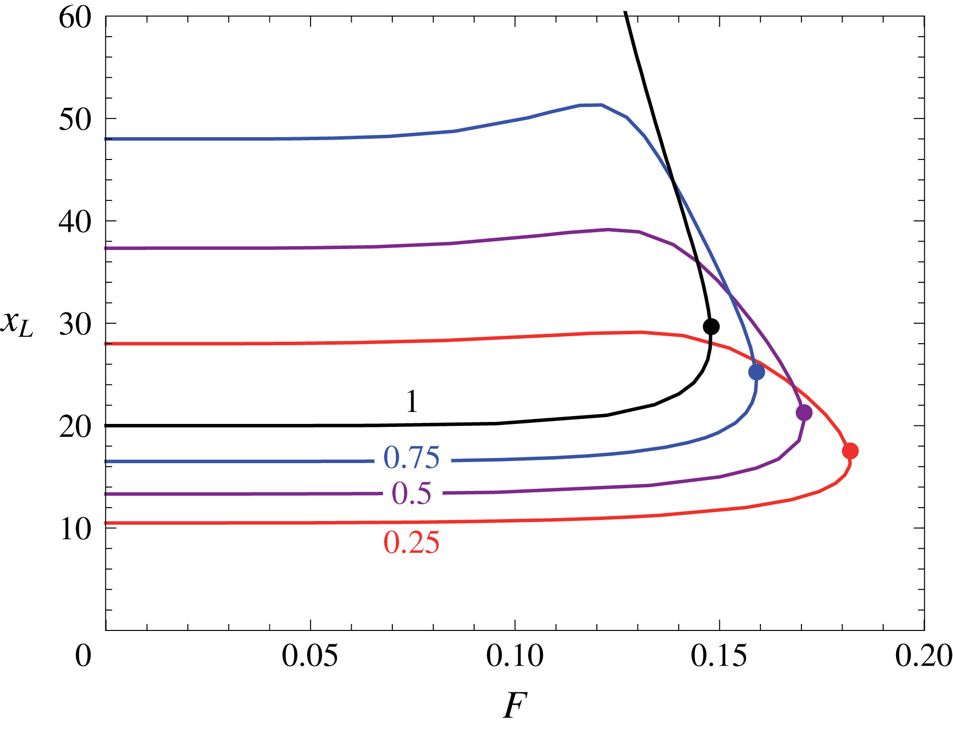
The deformation curve of viscous drops
 $(\unicode[STIX]{x1D706}\neq 0)$
in a linear flow
 $(H=0)$
, for different values of
 $n$
. Solid circles are placed at breakup points.

Figure 2 shows the deformation curve which has the form of a lobe starting at
 $\unicode[STIX]{x1D708}=n+1$
and ending at
 $\unicode[STIX]{x1D708}=2(n+1)$
for shear thinning drops
 $(n<1)$
or ending at
 $\unicode[STIX]{x1D708}=\infty$
for the Newtonian drop
 $(n=1)$
. The lobe is composed of two branches and separated by the bifurcation turning (breakup) point. A stability analysis performed in a consecutive report (Favelukis et al.
Reference Favelukis, Lavrenteva and Nir2006) reveals that the lower branch represents steady stable shapes while the unstable steady shapes are located at the upper branch. We observe that for the same viscous strength of low
 $(F)$
, Newtonian drops are more elongated than shear thinning drops, yet shear thinning drops are more difficult to break than Newtonian drops as they require larger critical values of
 $F$
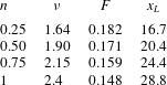
at the breakup point. Several physical properties at the breakup point are listed in table 1.
5.3 Newtonian drops
$(n=1)$
in a nonlinear flow
$(H\neq 0)$


The deformation and breakup of a Newtonian slender drop in a nonlinear extensional creeping flow was first suggested by Sherwood (Reference Sherwood1984) and recently reviewed and expanded by Favelukis (Reference Favelukis2016).
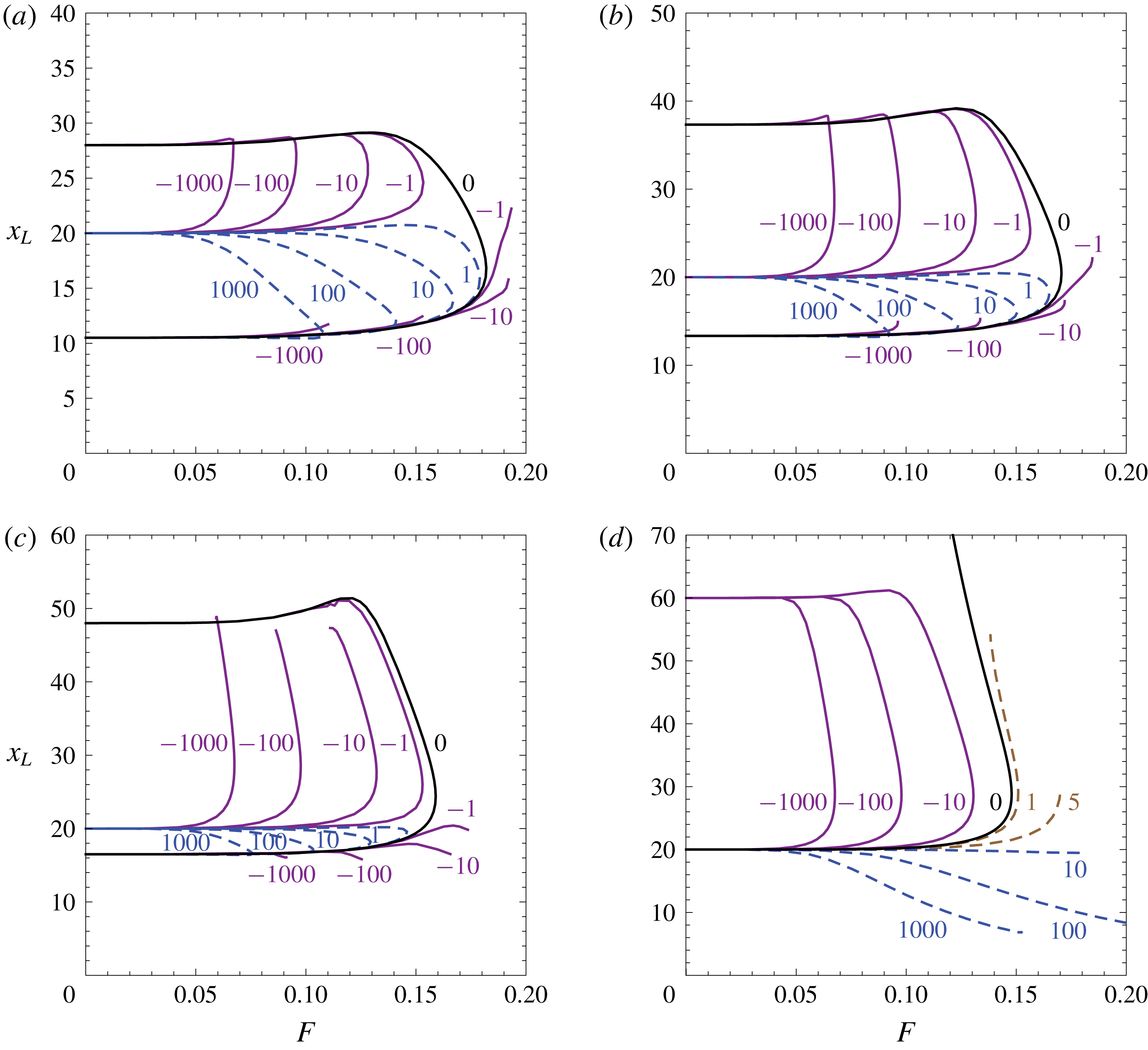
Deformation curve of shear thinning and Newtonian viscous drops
 $(\unicode[STIX]{x1D706}\neq 0,n\leqslant 1)$
, for different values of
 $H$
: (a)
 $n=0.25$
, (b)
 $n=0.50$
, (c)
 $n=0.75$
and (d)
 $n=1$
.

Parameters at the breakup point for a viscous drop
 $(\unicode[STIX]{x1D706}\neq 0)$
in a linear flow
 $(H=0)$
.

The deformation curve of a viscous Newtonian drop for different values of the parameter
 $H$
, is depicted in figure 3(d). First, the reader can easily locate the linear case
 $(H=0)$
, which is also plotted in figure 2. Time dependent studies performed by Favelukis et al. (Reference Favelukis, Lavrenteva and Nir2012) suggests that the breakup mechanism of a viscous Newtonian slender drop in a linear extensional creeping flow is by indefinite elongation in qualitative agreement with the experiments of Bentley & Leal (Reference Bentley and Leal1986).
When the flow is nonlinear
 $(H\neq 0)$
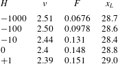
, we have four families of steady solutions, in which three of them are shown in figure 3(d). The first family, located to the left of the linear case, corresponds to
 $H<0$
,
 $x_{L}>20$
and
 $\unicode[STIX]{x1D708}>2$
. Here, the deformation curve, which behaves like the linear case, is composed of a lower stable branch, an upper unstable branch and a breakup point located at the bifurcation turning point, see also table 2. Contrary to the linear case, the upper branch is not extended to infinity but rather turns back on itself and ends at
 $F=0$
and
 $x_{L}=60$
, belonging to the singular point
 $\unicode[STIX]{x1D708}=4$
. Two breakup mechanisms were found for this family (Favelukis Reference Favelukis2016): indefinite elongation (low
 $|H|$
) and a centre pinching mode (high
 $|H|$
).
The next family of solutions, located to the right of the linear case
 $(H=0)$
, corresponds to
 $0<H<64/9=7.11$
,
 $x_{L}>20$
and
 $\unicode[STIX]{x1D708}>2$
. Some curves stop after the turning point
 $(H=1)$
and others stop before the turning point
 $(H=5)$
. The stability analysis done revealed that lines with bifurcation turning points are stable at the lower branch and unstable at the upper branch, with the turning point being the breakup point. Lines without a bifurcation turning point are stable everywhere. Time dependent studies on this family suggests a breakup mechanism reminding us of tip-streaming where a cusp is developed at the end of the slender drop (Favelukis Reference Favelukis2016).
The third family described in figure 3(d) is valid for
 $H>64/9$
,
 $x_{L}<20$
and
 $\unicode[STIX]{x1D708}<2$
. This family, which presents stationary drops which are fatter and shorter than the previous families, is stable everywhere. We are not sure whether the lines extend to infinity or just stop as a result of the numerical procedure. One common feature of all of the three families depicted in figure 3(d) is that the local radius of the drop decreases monotonically with increasing
 $x\,(x>0)$
. There is also a fourth family of solutions, corresponding to
 $H>64/9$
,
 $x_{L}>20$
and
 $\unicode[STIX]{x1D708}>2$
, which is not shown in this figure. This last family, suggesting strange drops with a maximum in the local radius besides the one at the centre of the drop, is all unstable.
Parameters at breakup point for a viscous Newtonian drop
 $(\unicode[STIX]{x1D706}\neq 0,n=1)$
, for the families of solutions with
 $H<64/9$
and bifurcation turning points.

5.4 Shear thinning drops
$(n<1)$
in a nonlinear flow
$(H\neq 0)$


Now that we are familiar with some deformation curves, we can proceed and explore the steady shapes of shear thinning drops
 $(n<1)$
in a nonlinear flow
 $(H\neq 0)$
which is the subject of this report. Following the procedure described in § 5.1, we produced in figure 3 deformation curves for different types of non-Newtonian shear thinning drops. The specific case of
 $n=1$
, is also incorporated here for comparison.
Consider any one of the shear thinning drops cases presented in figure 3(a–c). Let us observe first the linear case
 $(H=0)$
, already discussed in figure 2. It starts at
 $F=0$
,
 $\unicode[STIX]{x1D708}=n+1$
, and ends up once again at
 $F=0$
but with
 $\unicode[STIX]{x1D708}=2(n+1)$
. At these two points where
 $F=0$
, the half-length of the drop corresponds to an inviscid drop in a linear flow according to (4.2). When the flow is nonlinear
 $(H\neq 0)$
, we find two families of solutions depending on the sign of
 $H$
.
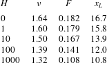
Parameters at the breakup point for a drop with
 $n=0.25$
and
 $H\geqslant 0$
.

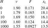
Parameters at the breakup point for a drop with
 $n=0.5$
and
 $H\geqslant 0$
.

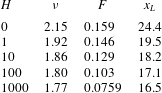
Parameters at the breakup point for a drop with
 $n=0.75$
and
 $H\geqslant 0$
.

The first family, corresponding to
 $H>0$
, starts at
 $F=0$
,
 $\unicode[STIX]{x1D708}=n+1$
and
 $x_{L}=4(n+2)(2n+3)/3$
, and ends at
 $F=0$
,
 $\unicode[STIX]{x1D708}=2$
and
 $x_{L}=20.$
It has the form of a lobe, composed of two branches which are separated by a bifurcation turning point. The stability analysis that we shall perform in the next section reveals, as expected, stable drops at the lower branch, unstable drops at the upper branch, and a breakup point at the turning point. A summary of properties at the breakup point, for this family of solutions and for different types of shear thinning drops, can be found in tables 3–5. For this family we can conclude the following: (i) stable shear thinning drops are less elongated than stable Newtonian drops; (ii) as the flow becomes more nonlinear or as
 $H$
increases, drop breakup is facilitated as it requires less critical values of
 $F$
; (iii) for a constant
 $H$
, as non-Newtonian effects increase or as
 $n$
decreases, breakup becomes more difficult since larger critical values of
 $F$
are required.
Steady-state drop shapes for
 $n=0.50$
and
 $H=+10$
.

The second family, belonging to
 $H<0$
, is divided into two unconnected subfamilies. The first subfamily, covering the range
 $(n+1)<\unicode[STIX]{x1D708}<2$
, contains a single open branch which starts at
 $F=0$
and
 $x_{L}=4(n+2)(2n+3)/3$
. Cases corresponding to low values of
 $|H|$
end closer to
 $\unicode[STIX]{x1D708}=2$
, while cases having large values of
 $|H|$
will end near
 $\unicode[STIX]{x1D708}=n+1$
. We are not sure about the end shape of this open branch since, near the end of the branch, the numerical slope at the end of the drop deviates from its asymptotic value given by (3.9). Nevertheless, the existence of a maximum value of
 $\unicode[STIX]{x1D708}$
or
 $F$
for this open branch is clear. Later on, our stability analysis will indicate that this open branch is stable everywhere. The second subfamily, corresponding to
 $2<\unicode[STIX]{x1D708}<2(n+1)$
, has the form of a lobe. It starts at
 $F=0$
,
 $x_{L}=20$
and ends at
 $F=0$
,
 $x_{L}=4(2n+3)(4n+5)/3$
. Note that for the specific case
 $n=0.75$
in figure 3(c), the lobe has a discontinuity section as result of numerical difficulties. We shall see that this subfamily is found to be unstable everywhere. The conclusions for this family are once again: (i) stable shear thinning drops are less elongated than Newtonian drops; (ii) as the flow becomes more nonlinear or as
 $|H|$
increases, drop breakup is facilitated as the maximum possible value of
 $F$
decreases; and (iii) for a constant
 $H$
, as non-Newtonian effects increase or as
 $n$
decreases, breakup becomes more difficult since larger critical values of
 $F$
are required.
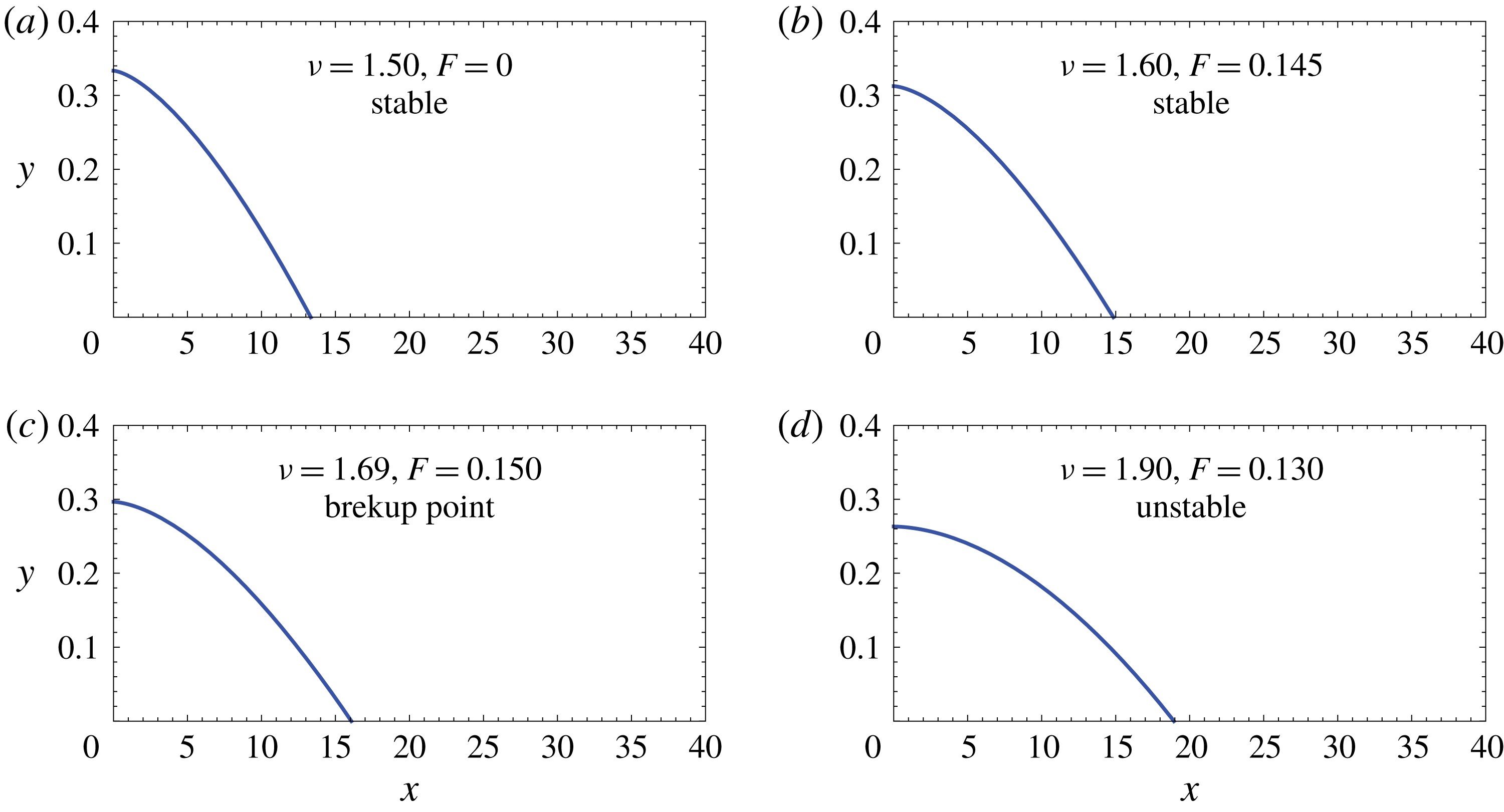
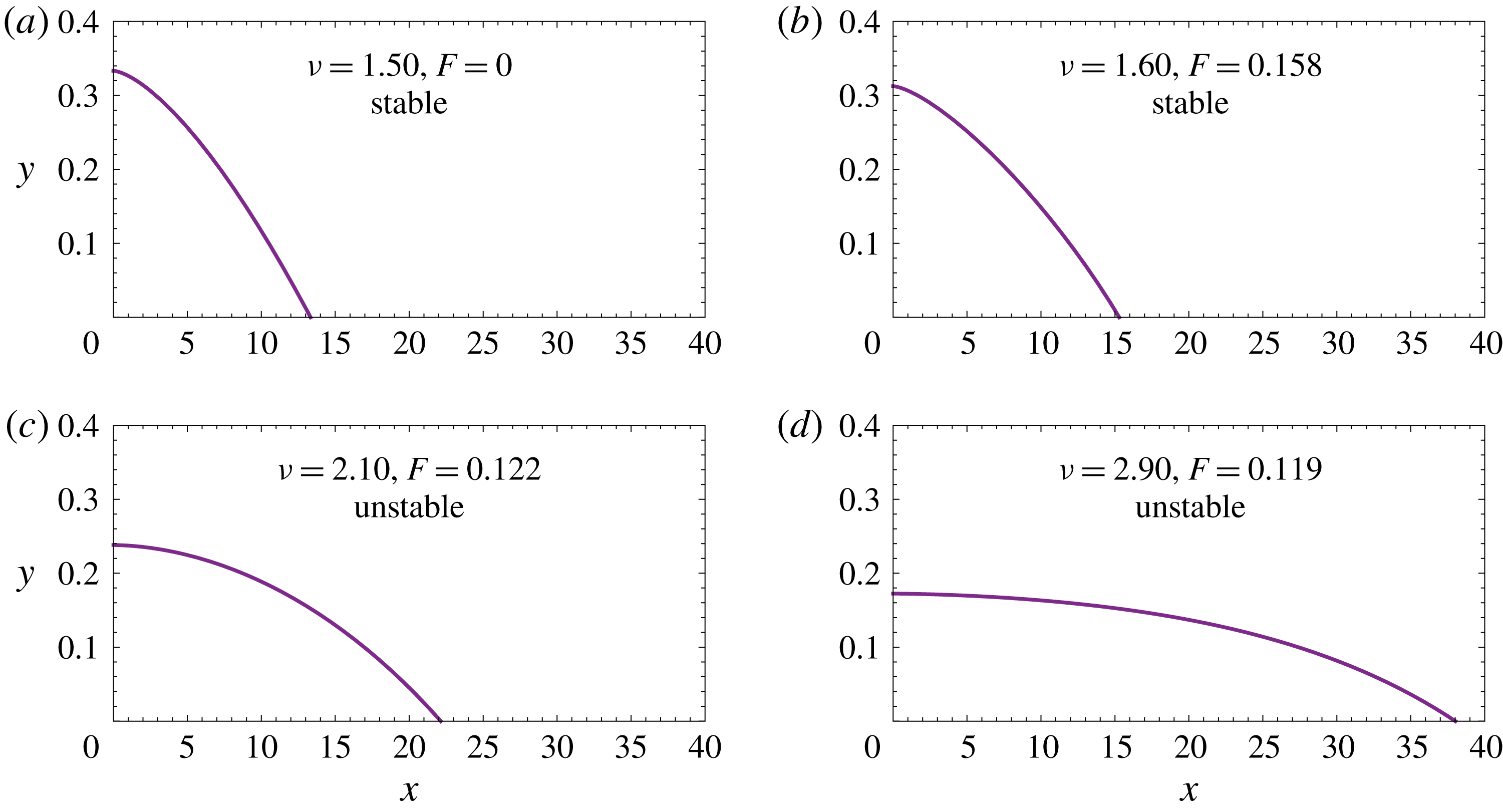
Finally, in figures 4 and 5 we describe steady-state drop shapes (stable and unstable) of shear thinning drops with
 $n=0.50$
, for
 $H=+10$
and
 $H=-10$
, respectively. For the simplest case of a steady Newtonian drop in a linear extensional flow, both stable and unstable drops are represented by a parabolic radius profile which monotonically decreases with the axial direction
 $(z\geqslant 0)$
. Also here, by looking at the shape, it is impossible to distinguish between stable and unstable stationary drops. Nevertheless, these steady unstable drops may break, in several types of breakup mechanisms such as centre pinching, indefinite elongation, or even tip streaming, as we saw for a Newtonian drop in a nonlinear extensional flow (Favelukis Reference Favelukis2016).
Steady-state drop shapes for
 $n=0.50$
and
 $H=-10$
.

5.5 The stability analysis
In order to locate the regions of stationary stable and stationary unstable drops, we shall perform here a stability analysis. Let the steady solution be
 $y_{0}(\unicode[STIX]{x1D719})$
, then we define a small axisymmetric disturbance
 $y_{1}(\unicode[STIX]{x1D719},t)$
as follows:
 $$\begin{eqnarray}y(\unicode[STIX]{x1D719},t)=y_{0}(\unicode[STIX]{x1D719})+y_{1}(\unicode[STIX]{x1D719},t),\quad y_{1}\ll y_{0}.\end{eqnarray}$$
Substituting the above definition into (5.1) and neglecting terms of
 $O(y_{1}^{2})$
or higher we obtain two equations. The first one is the steady form of (5.1), while the second equation reads
 $$\begin{eqnarray}\displaystyle & & \displaystyle 2(1+n)\frac{\unicode[STIX]{x2202}^{2}y_{1}}{\unicode[STIX]{x2202}\unicode[STIX]{x1D719}\unicode[STIX]{x2202}t}-2(1+n)\frac{1}{y_{0}}\frac{\text{d}y_{0}}{\text{d}\unicode[STIX]{x1D719}}\frac{\unicode[STIX]{x2202}y_{1}}{\unicode[STIX]{x2202}t}+2(1+n)^{2}[1+H\unicode[STIX]{x1D719}^{2/(1+n)}]\unicode[STIX]{x1D719}\frac{\unicode[STIX]{x2202}^{2}y_{1}}{\unicode[STIX]{x2202}\unicode[STIX]{x1D719}^{2}}\nonumber\\ \displaystyle & & \displaystyle \qquad +\,(1+n)\left\{2(1+n)+2(3+n)H\unicode[STIX]{x1D719}^{2/(1+n)}\right.\nonumber\\ \displaystyle & & \displaystyle \qquad -\left.\frac{1}{y_{0}}-4(1+n)[1+H\unicode[STIX]{x1D719}^{2/(1+n)}]\frac{\unicode[STIX]{x1D719}}{y_{0}}\frac{\text{d}y_{0}}{\text{d}\unicode[STIX]{x1D719}}\right\}\frac{\unicode[STIX]{x2202}y_{1}}{\unicode[STIX]{x2202}\unicode[STIX]{x1D719}}\nonumber\\ \displaystyle & & \displaystyle \qquad +\,\left\{\begin{array}{@{}l@{}}\displaystyle 2(1+n)^{2}[1+H\unicode[STIX]{x1D719}^{2/(1+n)}]\frac{\unicode[STIX]{x1D719}}{{y_{0}}^{2}}\left(\frac{\text{d}y_{0}}{\text{d}\unicode[STIX]{x1D719}}\right)^{2}+(1+n)\frac{1}{{y_{0}}^{2}}\frac{\text{d}y_{0}}{\text{d}\unicode[STIX]{x1D719}}\\ \displaystyle \quad +\,18H\unicode[STIX]{x1D719}^{(1-n)/(1+n)}+\frac{2nw[1+H\unicode[STIX]{x1D719}^{2/(1+n)}]^{n}}{{y_{0}}^{1+n}}\end{array}\right\}y_{1}\nonumber\\ \displaystyle & & \displaystyle \quad =\frac{4wn}{(1+n)}\frac{[1+H\unicode[STIX]{x1D719}^{2/(1+n)}]^{n-1}\unicode[STIX]{x1D719}^{-1/(1+n)}}{{y_{0}}^{2+n}}\frac{\unicode[STIX]{x2202}}{\unicode[STIX]{x2202}t}\int _{0}^{\unicode[STIX]{x1D719}}y_{0}y_{1}\unicode[STIX]{x1D719}^{-n/(1+n)}\,\text{d}\unicode[STIX]{x1D719}.\end{eqnarray}$$
Upon setting
 $y_{1}=g(\unicode[STIX]{x1D719})\exp (\unicode[STIX]{x1D6FF}t)$
into the last equation we obtain
 $$\begin{eqnarray}\displaystyle & & \displaystyle 2(1+n)^{2}[1+H\unicode[STIX]{x1D719}^{2/(1+n)}]\unicode[STIX]{x1D719}\frac{\text{d}^{2}g}{\text{d}\unicode[STIX]{x1D719}^{2}}\nonumber\\ \displaystyle & & \displaystyle \qquad +\,(1+n)\left\{2\unicode[STIX]{x1D6FF}-4(1+n)[1+H\unicode[STIX]{x1D719}^{2/(1+n)}]\frac{\unicode[STIX]{x1D719}}{y_{0}}\frac{\text{d}y_{0}}{\text{d}\unicode[STIX]{x1D719}}\right.\nonumber\\ \displaystyle & & \displaystyle \qquad +\left.2(1+n)+2(3+n)H\unicode[STIX]{x1D719}^{2/(1+n)}-\frac{1}{y_{0}}\right\}\frac{\text{d}g}{\text{d}\unicode[STIX]{x1D719}}\nonumber\\ \displaystyle & & \displaystyle \qquad +\,\left[\begin{array}{@{}l@{}}\displaystyle -2(1+n)\frac{\unicode[STIX]{x1D6FF}}{y_{0}}\frac{\text{d}y_{0}}{\text{d}\unicode[STIX]{x1D719}}+2(1+n)^{2}[1+H\unicode[STIX]{x1D719}^{2/(1+n)}]\frac{\unicode[STIX]{x1D719}}{{y_{0}}^{2}}\left(\frac{\text{d}y_{0}}{\text{d}\unicode[STIX]{x1D719}}\right)^{2}\\ \displaystyle \quad +\,(1+n)\frac{1}{{y_{0}}^{2}}\frac{\text{d}y_{0}}{\text{d}\unicode[STIX]{x1D719}}+18H\unicode[STIX]{x1D719}^{(1-n)/(1+n)}+\frac{2nw[1+H\unicode[STIX]{x1D719}^{2/(1+n)}]^{n}}{{y_{0}}^{1+n}}\end{array}\right]g\nonumber\\ \displaystyle & & \displaystyle \quad =\frac{4wn\unicode[STIX]{x1D6FF}}{(1+n)}[1+H\unicode[STIX]{x1D719}^{2/(1+n)}]^{n-1}\frac{\unicode[STIX]{x1D719}^{-1/(1+n)}}{{y_{0}}^{2+n}}\int _{0}^{\unicode[STIX]{x1D719}}y_{0}g\unicode[STIX]{x1D719}^{-n/(1+n)}\,\text{d}\unicode[STIX]{x1D719}.\end{eqnarray}$$
Following the double series expansion for the steady solution
 $y_{0}$
represented by (5.4), we assume a similar solution for the
 $g(\unicode[STIX]{x1D719})$
function
 $$\begin{eqnarray}g(\unicode[STIX]{x1D719})=\mathop{\sum }_{k=0}^{\infty }d_{k}\unicode[STIX]{x1D719}^{kp},\end{eqnarray}$$
with
 $p$
defined as in (5.4), except for the Newtonian case where
 $p=1$
. Furthermore, we can set
 $d_{0}=1$
without loss of generality (Acrivos & Lo Reference Acrivos and Lo1978). Once the coefficients
 $d_{k}$
and the function
 $g(\unicode[STIX]{x1D719})$
are determined, we can obtain the eigenvalues
 $\unicode[STIX]{x1D6FF}$
by solving the time derivative of the volume conservation, equation (2.17), which takes the form of
 $$\begin{eqnarray}\int _{0}^{x_{L}}y_{0}y_{1}\,\text{d}x=\int _{0}^{\unicode[STIX]{x1D719}_{L}}y_{0}g\unicode[STIX]{x1D719}^{-n/(1+n)}\,\text{d}\unicode[STIX]{x1D719}=0.\end{eqnarray}$$
For a specific value of
 $\unicode[STIX]{x1D708}$
there are many eigenvalues
 $\unicode[STIX]{x1D6FF}$
and we are interested in the one with the highest real part
 $Re\unicode[STIX]{x1D6FF}$
. It is clear that
 $Re\unicode[STIX]{x1D6FF}<0$
represents a stable solution, as small perturbations decay with time, while
 $Re\unicode[STIX]{x1D6FF}>0$
denotes an unstable physical situation. Thus, the point where
 $Re\unicode[STIX]{x1D6FF}=0$
is considered as the breakup point.
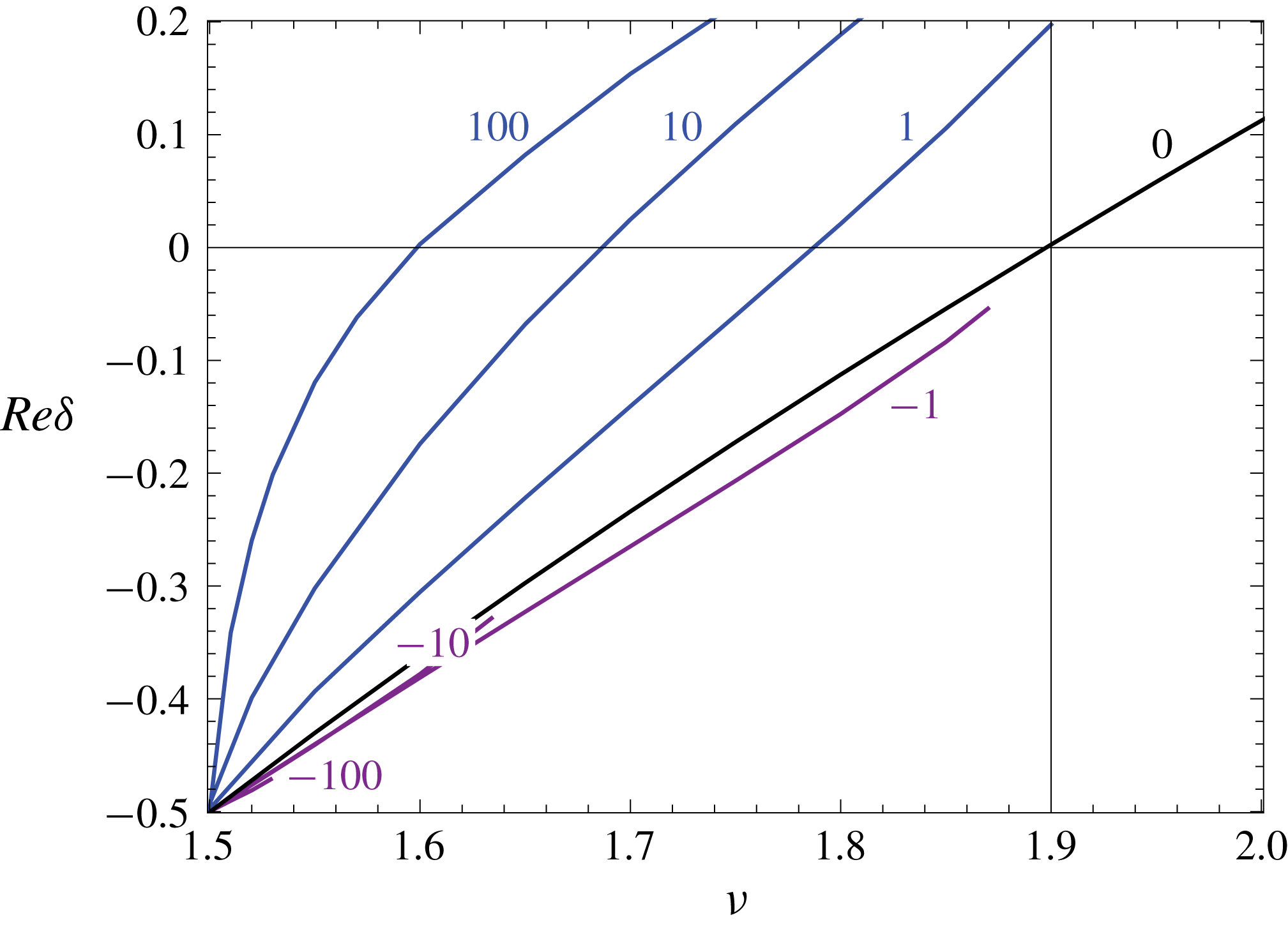
As an example, in figure 6 we present the highest eigenvalue
 $Re\unicode[STIX]{x1D6FF}$
as a function of
 $\unicode[STIX]{x1D708}$
for a shear thinning drop with
 $n=0.5$
. First, let us observe the linear case
 $(H=0)$
and its breakup point
 $(Re\unicode[STIX]{x1D6FF}=0)$
located at
 $\unicode[STIX]{x1D708}=1.90$
and
 $F=0.171$
corresponding to the bifurcation turning point, see also figure 2 and table 1 or table 4. To the left of the linear case we locate the first family of solutions in which
 $H>0$
and
 $(1+n)<\unicode[STIX]{x1D708}<2$
. The stability analysis for this family, which has the form of a lobe and is described in figure 3(b), confirms our earlier expectations of a lower stable branch, an upper unstable branch and the bifurcation turning point at the breakup point. A summary of the properties at the breakup point, for this family of solutions and for different type of shear thinning drops, was presented earlier in tables 3–5.
We continue with the next family of solutions corresponding to
 $H<0$
and located to the right of the linear case. Remember that this family is composed of two subfamilies, an open branch at
 $(n+1)<\unicode[STIX]{x1D708}<2$
and a lobe at
 $2<\unicode[STIX]{x1D708}<2(n+1)$
. The open branch, shown in the figure, is stable everywhere as
 $Re\unicode[STIX]{x1D6FF}<0$
, while for the lobe, not shown in the figure, we obtained
 $Re\unicode[STIX]{x1D6FF}>0$
and therefore it represents an unstable physical situation. Note that for the open branch, there is a maximum value of
 $\unicode[STIX]{x1D708}$
or
 $F$
. That is, beyond this value, a stable steady drop cannot exist and will break. Similar to the other family, as the flow becomes more nonlinear or as
 $|H|$
increases, drop breakup is facilitated since it requires fewer maximum values of
 $F$
, see also figure 3.
The stability of a shear thinning drop with
 $n=0.5$
, at different values of
 $H$
.

The stability analysis presented here and done on the creeping flow equations neglects the local acceleration which is very small in our case. Due to the small scale and high viscosity, typical to the creeping flow regime, and the dominance of viscous shear over capillary surface vibrations for such a slender body
 $(Ca\gg 1)$
, high frequency interfacial oscillations (as obtained by Sumanasekara, Azese & Bhattacharya Reference Sumanasekara, Azese and Bhattacharya2017 and Sumanasekara & Bhattacharya Reference Sumanasekara and Bhattacharya2017) are not expected for the present problem.
6 Conclusions
The deformation and stability of a power-law non-Newtonian slender drop in a nonlinear axisymmetric extensional and creeping flow has been theoretically studied. The problem is governed by four dimensionless numbers, the capillary number
 $(Ca\gg 1)$
, the viscosity ratio
 $(\unicode[STIX]{x1D706}\ll 1)$
, the power-law index
 $(n)$
and the nonlinear intensity of the flow
 $(|E|\ll 1)$
. A further exploration suggests that the number of dimensionless governing parameters can be reduced from four to three having the order of magnitude of 1, namely the viscous strength of the flow
 $F=Ca\unicode[STIX]{x1D706}^{1/3(1+n)}$
, the nonlinear strength of the flow
 $G=Ca^{4}E$
, which can be positive or negative, and the power-law index
 $n$
.
A theory for a slender Newtonian drop in a nonlinear axisymmetric extensional creeping flow was first suggested by Sherwood (Reference Sherwood1984) and recently reviewed and expanded by Favelukis (Reference Favelukis2016). In this report we further expand the theory by including non-Newtonian effects to the fluid inside the drop. We follow Acrivos & Lo (Reference Acrivos and Lo1978) and define the radius at the centre of the drop as
 $1/(2\unicode[STIX]{x1D708})$
, with
 $\unicode[STIX]{x1D708}$
being related to the steady pressure at the centre of the drop. Let a parameter
 $H$
represent the ratio of the nonlinear strength of the flow to the viscous strength of the flow
 $H=G/F^{6}$
. Thus,
 $H=0$
corresponds to a viscous drop
 $(\unicode[STIX]{x1D706}\neq 0)$
in a linear extensional flow
 $(G=0)$
, while
 $H\rightarrow \pm \infty$
represents an inviscid drop
 $(\unicode[STIX]{x1D706}=0)$
in a nonlinear extensional flow
 $(G\neq 0)$
.
The steady-state solution close to the end of the drop suggests that only Newtonian and shear thinning drops
 $(n\leqslant 1)$
are possible. These slender drops with or without nonlinear effects have pointed ends. The shape of the drop, which is obtained by assuming a solution in the form of a double series expansion about the centre of the drop, suggests singular points located, in ascending order, at
 $\unicode[STIX]{x1D708}=(n+1)$
,
 $\unicode[STIX]{x1D708}=2$
,
 $\unicode[STIX]{x1D708}=2(n+1)$
,
 $\unicode[STIX]{x1D708}=4$
and so on. The solution reveals a deformation curve containing multiple lobes and based on past experience in this subject, we concentrated our search to low values of
 $\unicode[STIX]{x1D708}$
and in drops shapes where the local radius decreases monotonically
 $(z\geqslant 0)$
, as there stable drops are expected to be found.
For a Newtonian drop
 $(n=1)$
, three main families of solutions exist. The first family, located at
 $\unicode[STIX]{x1D708}>2$
and
 $H<0$
, has a deformation curve which is composed of a lower stable branch, an upper unstable branch and a breakup point located at the bifurcation turning point. In the second family, corresponding to
 $\unicode[STIX]{x1D708}>2$
and
 $0<H<64/9$
, some deformation curves stop after the turning point and others stop before the turning point. Lines with bifurcation turning points are, as expected, stable at the lower branch and unstable at the upper branch, with the turning point being the breakup point. Lines without a bifurcation turning point are stable everywhere. The third family, located at
 $\unicode[STIX]{x1D708}<2$
and
 $H>64/9$
, is stable everywhere.
A complicated picture is also revealed when dealing with shear thinning drops
 $(n<1)$
. Here, two families of solutions with a monotonically decreasing local radius were obtained. The first family, corresponding to
 $H>0$
and located where
 $(n+1)<\unicode[STIX]{x1D708}<2$
, has the form of a lobe composed of a lower stable branch, an upper unstable branch and a breakup point at the bifurcation turning point. The second family, belonging to
 $H<0$
, is divided into two unconnected regions, a lower stable region,
 $(n+1)<\unicode[STIX]{x1D708}<2$
, described by a stable open branch, and an upper unstable region,
 $2<\unicode[STIX]{x1D708}<2(n+1)$
, having the form of a lobe with a bifurcation turning point. The stability and the breakup conclusions for these two families are based on a stability analysis to small perturbation also executed in this report. Our findings suggest that shear thinning drops are less elongated and more difficult to break than Newtonian drops. Also, as
 $|H|$
increases or the flow becomes more nonlinear, in terms of the viscous strength of the flow
 $F$
, breakup is facilitated.
High viscosity liquids such as polymer melts, foods, cosmetics and pharmaceutical products exhibit non-Newtonian effects such as shear thinning and elasticity. Emulsions made from these materials are usually processed in mixing devices undergoing shear, extensional, but in general, much more complicated flows such as nonlinear flows. The work presented here attempts to explain the deformation and stability of slender drops in an extensional flow when non-Newtonian fluids and nonlinear flows appear simultaneously. Hopefully, the results of this report will provide a better understanding in the design of such rotary equipment.
Acknowledgements
This research was supported by Shenkar College of Engineering and Design. The author would like to thank Professor A. Nir from the Technion – Israel Institute of Technology, for very useful discussions.