Nomenclature
- a, b
-
respectively represent the major axis and minor axis
- A
-
the area distribution of the inlet duct
- D
-
outlet diameter
- F y
-
component of the vertical force acting on the ice-debris
- L
-
diffuser length
- L I
-
the inertia tensor of ice
- m
-
mass of the ice
- M B
-
moment vector of the ice
- M G
-
moment vector of the ice in the body coordinate system
- n
-
super-ellipse parameter
- R
-
transformation matrix from inertial to body coordinate
- S 1/4
-
quarter of the area covered by a super-ellipse curve
-
 $\boldsymbol{v}$
-
velocity of the fluid
-
$\bar{\boldsymbol{v}}_G$
-
the translational motion of the centre of gravity


Greek symbol
-
$\Delta y$
-
longitudinal offset
-
$\mu $
-
molecular viscosity
- ρ
-
density
-
$\phi $
,
$\theta $
,
$\psi $
-
Euler angles that represent the rotations around the z, y and x
-
${\bar{\boldsymbol{\omega }}_B}$
-
the angular motion of the ice-debris


Subscripts
- CG
-
centre of gravity
1.0 Introduction
The ability of aircraft engines to resist foreign object impact is an important assessment indicator in the engine development process. For engines equipped with complex S-shaped inlet ducts, the influence of the inlet duct on the behaviour of foreign objects must be considered. Since S-shaped inlet contribute to enhancing the stealth performance of aircraft, advanced military fighters often adopt this design. During high-altitude flight, the high-power turbofan engine matched with the S-shaped inlet generates a strong negative pressure near the inlet of the engine, causing hailstones and ice-debris floating in the air to be sucked into the inlet duct. In addition, ice-debris shedding inside the inlet duct will also move downstream under the action of high-speed airflow and are likely to collide with rotating components such as the engine fan, causing serious damage or even leading to engine surges, flameouts, etc., posing a serious threat to flight safety [Reference Ozgen and Cambek1]. Therefore, analysing the trajectory of ice-debris in the S-shaped inlet in advance to provide data support for foreign object impact damage experiments has become one of the key measures to prevent Foreign Object Damage (FOD) issues.
In the 1950s, foreign scholars such as Kaufman pioneered research on the impact of foreign object damage on the fatigue strength of jet engine compressor rotor blades [Reference Kaufman and Meyer2]. With the development of computational fluid dynamics (CFD) technology, numerical simulation has been able to replace experimental studies on FOD issues. Earlier simulations were mostly based on erosion models to investigate the motion characteristics of foreign objects in FOD events and the metal behaviour of engine components [Reference Wakeman and Tabakoff3–Reference Hamed, Tabakoff and Wenglarz5]. Nowadays, numerical simulations can replace some wind tunnel tests, and research on the fatigue strength of engine rotating components through simulated FOD damage tests is gradually increasing [Reference Zhang, Du and Ren6–Reference Jacobs, Harman, Ladani, Das and Orifici8].
Research on ice trajectory in FOD events is mainly divided into external ingested ice and internal shedding ice. As current studies mostly focus on nacelle engines in civil aviation, there is more research on external ingested ice trajectories. Hinson et al. [Reference Chandrasekharan and Hinson9] demonstrated through calculations of two models of commercial aircraft that changes in fuselage length do not increase the risk of engine ice ingestion. Papadakis et al. [Reference Papadakis, Yeong, Suares and Jacob10–Reference Papadakis, Yeong, Shimoi and Wong12] described a methodology that integrates experimental aerodynamic characteristics, computational fluid dynamics, trajectory analysis and Monte Carlo methods to compute the trajectories of large ice particles shed from aircraft surfaces. This approach aims to enhance the prediction of ice particle randomness and aerodynamic behaviour, particularly in assessing the risk of engine ingestion and generating probability distribution maps. Deschenes et al. [Reference Deschenes, Baruzzi, Lagace and Habashi13] presented a fully CFD-based methodology within the FENSAP-ICE system for tracking ice particle trajectories using a Monte Carlo statistical approach and six degrees-of-freedom particle-tracking, with forces and moments determined from precomputed aerodynamic coefficients, and validated through comparison with experimental data for a complete aircraft geometry. Additionally, Chen et al. [Reference Chen, Dong, Wang and Fu14] discussed factors influencing ice shedding and fragmentation by establishing a numerical model coupling the surface damage of engine fan blades with ice and ice fragmentation itself. Védie et al. [Reference Védie, Morency and Kubler15] addressed the challenge of predicting ice particle trajectories in inflight aircraft de-icing systems by proposing a method to estimate the number of Monte Carlo samples required for a desired accuracy, validating the approach through comparison with existing experimental and numerical results, and demonstrating agreement with previous studies.
Recent advancements by scholars like Beaugendre et al. [Reference Beaugendre, Nouveau, Costes, Wervaecke and Kilian16] have incorporated the coupling of aerodynamics and rigid body dynamics to accurately simulate ice trajectories on wing leading edges, validating their findings through wind tunnel experiments using the overset mesh method. Ayan et al. [Reference Ayan and Özgen17] integrated models for solid- and mixed-phase icing, developed within the European Commission’s HAIC project, into a numerical tool comprising flow-field, particle trajectory, thermodynamic and ice accretion modules, and validates the tool against experimental data for various geometries, showing promising agreement with experimental results. Furthermore, Sengupta et al. [Reference Sengupta, Raj, Cho, Son, Yoon, Yee and Myong18] developed a methodology for predicting ice accretion, break-off, and shedding trajectories in rotorcraft flow fields, incorporating aerodynamic databases, CFD analyses and six degrees-of-freedom (6-DOF) trajectory simulations, and highlights the critical role of rotor wakes and ice fragment shape in determining the potential hazards to engine intake and tail rotor systems.
Due to the simple geometric characteristics of nacelle engine inlets, the aforementioned studies primarily focus on whether external ice fragments are ingested into the engine and their landing positions on the engine fan. There is relatively limited research on the trajectories of ice-debris within complex geometric inlet ducts. Similar research conducted by Mi et al. [Reference Mi and Zhan19] investigated the behaviour of spherical and hexahedral metallic foreign objects in turboprop engine intake systems with a bypass duct, finding that such objects, especially hexahedral ones, significantly impact intake performance before exiting through the bypass duct. In a subsequent study [Reference Mi20], they explored the effects of ice-debris and hailstones at the inlet, revealing that large ice chunks can cause severe impacts on the duct wall, reducing pressure recovery and increasing distortion at the junction with the bypass duct, thereby compromising engine safety.
Current research mainly relies on the database method or dynamic mesh to analyse the trajectory of external ice-debris, primarily focusing on civil nacelle engines and turboprop engine intakes. However, this paper introduces a novel approach by employing 6-DOF overset mesh technology, which effectively avoids the mesh distortion and computational burden typically associated with dynamic mesh methods. Moreover, the accuracy of the model is validated through experimental data on the aerodynamic motion of ice-debris within the channel, significantly enhancing computational efficiency. Additionally, a dorsal S-shaped inlet with a length of 6.74m is constructed, and the aerodynamic behaviour of internal ice-debris is studied using the Euler-Lagrange gas-solid two-phase method. This study mainly investigates two scenarios: one where external ice is ingested with an initial velocity, and another where ice delaminates from the inner wall of the inlet duct. By analysing these two cases, the research aims to acquire information on the trajectories and impact velocities of ice-debris. The findings provide a fundamental reference for optimising complex aircraft inlet structures and advancing future studies on foreign object damage in S-shaped inlets, thereby ensuring flight safety and significantly reducing the risk of foreign object damage incidents.
2.0 Numerical models
2.1 Design of the geometry model for a dorsal S-shaped inlet
A conventional parameterised design is adopted to construct the geometry of the dorsal S-shaped inlet. Figure 1 illustrates the internal passage of a conventional subsonic S-shaped inlet. This paper focuses on the dynamic behaviour of ice-debris inside the inlet duct, thus the S-shaped inlet used mainly involves the transition section, diffuser and export transition section for drawing.
As shown in Fig. 1, to avoid the non-uniformity of high Mach number airflow in the throat and to prevent separated airflow downstream of the intake from entering the engine, this study introduces straight transition sections both after the throat and at the intake duct outlet. The length of the former is equal to 0.5 times the equivalent diameter of the throat, while the length of the latter is equal to the diameter of the intake duct outlet [Reference Zhang, Wang and Lum22]. For the design of the diffuser, besides the inlet and outlet parameters, the variation law of the centreline and area distribution, as well as the determination of cross-sectional parameters (referred to as diffuser shape parameters), are critical aspects of the design. They determine the airflow conditions inside the duct and whether the inner wall of the inlet duct is smooth enough.
2.1.1 Design of the inlet and outlet parameters for the diffuser
The present study intends to conduct simulation research on a dorsal S-shaped inlet with an elliptical inlet transitioning to a circular outlet, where the aspect ratio of the elliptical inlet is 2:1. To approximate the inlet duct of military aircraft, parameters such as inlet duct outlet area, diffuser length and diffusion ratio are referenced from the design of the YF-16 aircraft inlet duct [Reference Hawkins23]. The final settings for the inlet duct include an outlet diameter of 0.9m, a diffuser length of 5.5m and a diffusion ratio of 1.3. The determination of the longitudinal offset relies on the outlet diameter of the inlet duct. Hence, the longitudinal offset is set to be 1 times the diameter of the outlet diameter in this study [Reference Zhang21]. It should be noted that the 5.5m refers only to the length of the diffuser section of the inlet duct. The overall length of the inlet duct, which includes the inlet transition section, diffuser section, and outlet sections, is calculated to be 6.74m. In summary, the inlet and outlet parameters of the dorsal S-shaped inlet designed in this study are shown in Table 1. The key design parameters, such as the longitudinal offset, outlet diameter and diffuser length, are indicated in Fig. 2. Additionally, in Fig. 2, the red and purple highlighted lines represent the centreline and section lines of the duct, respectively. Detailed design specifications are provided in section 2.1.2.
Inlet and outlet parameters of the diffuser

The schematic of subsonic S-shaped inlet [Reference Zhang21].

The schematic of key parameters of 3D S-shaped inlet.

2.1.2 Design of the diffuser shape parameters
The variations in the centreline and area distribution commonly adopt three patterns proposed in Ref. (Reference Lee and Boedicker24), corresponding to the three patterns shown in Equation (1). Figure 3 provides a detailed illustration of the different centreline and area distribution curves.
 \begin{align}{{{\left\{ \begin{array}{l}{\rm{Centerline\; \# 1\; }}y = \Delta y\Big[ - 3{\Big(\dfrac{x}{L}\Big)^4} + 4{\Big(\dfrac{x}{L}\Big)^3}\Big]\\[6pt]{\rm{Centerline\; \# 2\; }}y = \Delta y\Big[3{\Big(\dfrac{x}{L}\Big)^2} - 2{\Big(\dfrac{x}{L}\Big)^3}\Big]\\[6pt]{\rm{Centerline\; \# 3\; }}y = \Delta y\Big[3{\Big(\dfrac{x}{L}\Big)^4} - 8{\Big(\dfrac{x}{L}\Big)^3} + 6{\Big(\dfrac{x}{L}\Big)^2}\Big]\end{array} \right.\left\{ \begin{array}{l}{\rm{Area\ Distribution\; \# 1\; }}\dfrac{A}{{{A_1}}} = \Big(\dfrac{{{A_2}}}{{{A_1}}} - 1\Big)\Big[ - 3{\Big(\dfrac{x}{L}\Big)^4} + 4{\Big(\dfrac{x}{L}\Big)^3}\Big] + 1\\[6pt]{\rm{Area\ Distribution\; \# 2\; }}\dfrac{A}{{{A_1}}} = \Big(\dfrac{{{A_2}}}{{{A_1}}} - 1\Big)\Big[3{\Big(\dfrac{x}{L}\Big)^2} - 2{\Big(\dfrac{x}{L}\Big)^3}\Big] + 1\\[6pt]{\rm{Area\ Distribution\; \# 3\; }}\dfrac{A}{{{A_1}}} = \Big(\dfrac{{{A_2}}}{{{A_1}}} - 1\Big)\Big[3{\Big(\dfrac{x}{L}\Big)^4} - 8{\Big(\dfrac{x}{L}\Big)^3} + 6{\Big(\dfrac{x}{L}\Big)^2}\Big] + 1\end{array} \right.\!\!.}}}\end{align}
The centreline and area distribution of the diffuser section.

Where x and y, respectively, represent the horizontal and vertical coordinates of centreline;
 $\Delta y$
denotes the longitudinal offset; L represents the length of the diffuser; A is the area distribution of the inlet duct; A
2/A
1 represents the diffusion ratio of the duct.
Numerous experimental and numerical results indicate that the #3 centreline minimises pressure distortion at the outlet and ensures a uniform diffusion ratio, reducing airflow separation. Additionally, for ducts with flatter inlets or larger longitudinal offsets, the #3 centreline facilitates an earlier airflow direction change, aligning the flow with the engine axis at the outlet. Since this study designs an elliptical inlet, the #3 centreline and corresponding area distribution are ultimately chosen.
The transition of the inlet duct’s cross-sectional shape is controlled using the super-ellipse equation, with its key parameter n determining the smoothness of the inner wall [Reference Shu, Xue and Zhu25]:
 \begin{align}{\left(\frac{{{x^2}}}{{{a^2}}}\right)^{\frac{n}{2}}} + {\left(\frac{{{y^2}}}{{{b^2}}}\right)^{\frac{n}{2}}} = 1.\end{align}
Where a, b and n are positive real numbers. The parameters of the major axis a and minor axis b are derived based on the chosen #3 area distribution, allowing for the calculation of cross-sectional areas and smooth transitions along the duct. It is possible to obtain the parameter n for any cross-section through the inverse solution of the definite integral equation:
 \begin{align}{S_{1/4}} = ab{\int_0^1 {(1 - {y^n})} ^{\frac{1}{n}}}dy.\end{align}
Where
 ${S_{1/4}}$
represents the area formed by the super-ellipse curve in the first quadrant with the coordinate axes.
By combining the inlet and outlet parameters with the cross-sectional shapes, seven control lines were generated to model the S-shaped inlet using SolidWorks software. Transition sections were added at the front and rear of the diffuser, resulting in the dorsal S-shaped inlet design, as shown in Fig. 4. The diagram illustrates the geometric configuration of the inlet duct, with critical parameters highlighted in red. These parameters include the longitudinal offset, outlet diameter, diffuser section length and section position. By systematically modifying these parameters, the inlet duct can achieve a suitable structure and good aerodynamic performance to meet different operational requirements.
Geometry of the dorsal S-shaped inlet used in this study.

2.2 Computational method
2.2.1 Overset mesh technology of rigid body motion
The movement of ice-debris in the high-speed flow field of the inlet duct is a crucial issue. Currently, methods for simulating rigid body motion mainly include sliding mesh, dynamic mesh and overset mesh. Sliding mesh is often used for studying rigid body motion with fixed trajectories. Although dynamic mesh can achieve the movement between objects by mesh deformation and stretching, the computation process often leads to severe mesh distortion and negative volume mesh generation, resulting in poor computational results while significantly consuming computational resources. The overset mesh involves interpolation within two or more mutually nested computational domains. It couples different computational domains by exchanging data between the acceptor cells of one domain and the donor cells of another domain.
As a method of domain decomposition and mesh assembly, overset mesh integrates the advantages of sliding mesh and dynamic mesh. Compared to sliding mesh, overset mesh ensures that meshes in different regions within the computational domain do not interfere with each other and allows for the use of different types of meshes, thereby reducing the difficulty of mesh generation while maintaining mesh quality. Additionally, during the computation process, overset mesh only updates the boundary meshes of the over-set regions as objects move, without generating mesh deformation, thus overcoming the mesh distortion issues encountered with dynamic mesh updates [Reference Secco and Martins26]. Clearly, overset mesh technology is well-suited for the long-distance and irregular motion of ice-debris in this study.
2.2.2 Mesh division of the inlet duct containing ice-debris
The overset mesh used in this study consists of two sets of nested meshes. The fluid domain of the inlet duct belongs to the background region, while the custom region containing the ice-debris belongs to the overset region. Figure 5 illustrates the mesh division of the inlet duct containing ice-debris. The subsequent mesh division methods for ice-debris at different positions in the inlet duct are consistent and will not be repeated.
Mesh generation of inlet duct.

The overset mesh allows for the utilisation of different types of meshes in the background and overset domains. In this study, the background region adopts ‘poly-hexcore’ mesh, with the interior divided into cubic meshes and the boundary meshes transitioning with polyhedral meshes. The overset region is partitioned using Hexahedron mesh. Both regions mostly employ orthogonal hexahedral meshes with high-quality. Therefore, the mesh division method can significantly improve mesh quality while conserving computational resources. Additionally, this study employs polyhedral prism mesh to generate eight layers of boundary layer near the wall, with a total thickness of 14.8mm and a growth rate of 1.12.
Figure 6 illustrates the mesh distribution near the ice-debris on the z = 0 plane before and after the establishment of the overset mesh, with the red box indicating the boundary of the overset region. Before establishing the overset mesh, the background domain has not undergone ‘mesh marking’ and ‘hole cutting’ processing. After the generation of the overset mesh, inactive cells are removed from the central region and information transfer within the computational domain relies mainly on the meshes in the boundary region of the overset part.
(a) Initial mesh; (b) The generated overset mesh.

2.3 Numerical methodology
The SST k-ω model is employed to simulate the flow field inside the inlet duct. This model incorporates the effects of turbulent shear stress transport in the definition of turbulent viscosity, making the SST k-ω model more accurate and widely applicable compared to other two-equation RANS models. Jin et al. [Reference Jin, Taghav and Farokhi27] also used this turbulence model to simulate compressible viscous flow in an S-shaped inlet duct, verifying the reliability of the model. The transport equations for turbulent kinetic energy k and specific dissipation rate ω are expressed as follows:
 \begin{align}\frac{\partial }{{\partial t}}(\rho k) + \frac{\partial }{{\partial {x_i}}}\left( {\rho k{u_i}} \right) = \frac{\partial }{{\partial {x_j}}}\left(\frac{{\partial k}}{{\partial {x_j}}}\left(\mu + \frac{{{\mu _t}}}{{{\sigma _k}}}\right)\right) + {G_k} - \rho {\beta ^*}k\omega + {G_b},\end{align}
 \begin{align}\frac{\partial }{{\partial t}}(\rho \omega ) + \frac{\partial }{{\partial {x_i}}}\left( {\rho \omega {u_i}} \right) = \frac{\partial }{{\partial {x_j}}}\left(\frac{{\partial \omega }}{{\partial {x_j}}}\left(\mu + \frac{{{\mu _t}}}{{{\sigma _\omega }}}\right)\right) + {G_\omega } - \rho \beta {\omega ^2} + {D_\omega } + {G_{\omega b}}.\end{align}
The interaction forces between the gas and solid phases are accounted for through source terms in the momentum equations:
 \begin{align}\frac{\partial }{{\partial t}}(\rho {\rm{v}}) + \nabla \cdot (\rho \boldsymbol{vv}) = - \nabla p + \nabla \cdot (\bar{\bar{\tau}}) + \rho \boldsymbol{g} - {a_d}\boldsymbol{v} + {\boldsymbol{F}_{fluid}}.\end{align}
Where,
 $\bar{\bar{\tau}} = \mu [(\nabla \boldsymbol{v} + \nabla {\boldsymbol{v}^T}) - \frac{2}{3}\nabla \cdot \boldsymbol{v}I]$
represents the stress tensor;
 $ - {a_d}\boldsymbol{v}$
is the linear damping force; and the fluid force is defined by Equation (7).
 \begin{align}{\boldsymbol{F}_{fluid}} = \sum {{p_f}{\boldsymbol{a}_f}} - \sum {{\tau _f}{\boldsymbol{a}_f}} .\end{align}
Where,
 ${p_f}$
and
 ${\tau _f}$
are, respectively, the pressure and shear stress acting on face f;
 ${\boldsymbol{a}_f}$
is the area vector of face f.
2.4 6-DOF governing equation of ice-debris
The 6-DOF solver uses the ice-debris’ forces and moments in order to compute the translational and angular motion of the centre of gravity of an object. The governing equation for the translational motion of the centre of gravity is solved for in the inertial coordinate system:
 \begin{align}{\dot{\bar{\boldsymbol{v}}}_G} = \frac{1}{m}\sum {{\boldsymbol{f}_G}}, \end{align}
where
 $\dot{\bar{\boldsymbol{v}}}_G$
is the translational motion of the centre of gravity, m is the mass, and
 ${\boldsymbol{f}_G}$
is the force vector due to gravity.
The angular motion of the ice-debris,
 ${\bar{\boldsymbol{\omega}}_B}$
, is more easily computed using body coordinates:
 \begin{align}{\bar{\boldsymbol{\omega}}_B} = {L_{\rm{I}}}^{ - 1}\left(\sum {{\boldsymbol{M}_B}} - {{\boldsymbol{\omega }}_B} \times {L_I}{{\boldsymbol{\omega }}_B}\right),\end{align}
where L
I
is the inertia tensor,
 ${\boldsymbol{M}_B}$
is the moment vector of the body, and
 ${{\boldsymbol{\omega }}_B}$
is the rigid body angular velocity vector.
The moments are transformed from inertial to body coordinates using:
 \begin{align}{\boldsymbol{M}_B} = \boldsymbol{R}{\boldsymbol{M}_G},\end{align}
where, R represents the following transformation matrix:
 \begin{align}\left[ {\begin{array}{c@{\quad}c@{\quad}c}{{C_\theta }{C_\psi }} & {}{{C_\theta }{S_\psi }}& {}{ - {S_\theta }}\\{{S_\phi }{S_\theta }{S_\psi } - {C_\phi }{S_\psi }} {}&{{S_\phi }{S_\theta }{S_\psi } + {C_\phi }{C_\psi }}& {}{{S_\phi }{C_\theta }}\\{{C_\phi }{S_\theta }{C_\psi } + {S_\phi }{S_\psi }} {}&{{C_\phi }{S_\theta }{S_\psi } - {S_\phi }{C_\psi }}& {}{{C_\phi }{C_\theta }}\end{array}} \right],\end{align}
where, in generic terms,
 ${C_i} = \cos\! (i)$
and
 ${S_i} = \sin\! (i)$
. The angles
 $\phi $
,
 $\theta $
, and
 $\psi $
are Euler angles that represent the rotations around the z, y and x axes, respectively.
After the angular and the translational accelerations are computed from Equation (8) and Equation (9), the rates are derived by numerical integration [Reference Snyder, Koutsavdis and Anttonen28]. The angular and translational velocities are used in the dynamic mesh calculations to update the ice-debris position.
3.0 Results and discussion
3.1 Model validation
To ensure the accurate prediction of the trajectory of ice-debris within the inlet duct using a 6-DOF overset mesh numerical model, experimental trajectory data of ice-debris, generated by Papadakis et al. in the WSU Beech Memorial Wind Tunnel, were used for validation [Reference Papadakis, Yeong, Shimoi and Wong12]. The experiment involved a small wind tunnel with a single-return closed-loop facility, where the test section measured 7-ft in height, 10-ft in width, and 12-ft in length. High-speed cameras captured the rolling behaviour of the ice-debris within the airflow channel, and the corresponding centroid trajectories were obtained. Under the assumption that ice collisions and fragmentation were not considered, this experimental data provided accurate validation for the trajectory simulation of the ice in unsteady turbulence within the inlet duct.
The researchers in the above experiment used high-speed video and a grid attached to the tunnel wall to record the ice trajectories (as shown in Fig. 7). They studied the aerodynamic behaviour of ice-debris with different shapes within the airflow channel. In this study, we selected trajectory data for the rectangular-shaped ice-debris under the RFP6 case for model validation. The mass parameters of the ice, flow field parameters and other key details are provided in Table 2.
The key parameters of the experiment under the RFP6 case

Side view of experimental device and inertial coordinate system.

The overset mesh and adaptive mesh are applied to establish the information transfer between the ice and the fluid domain, and the overset mesh at the y = 0 plane of the ice centre is shown in Fig. 8. The velocity inlet and pressure outlet boundary conditions are applied to the upstream and downstream of the fluid domain, respectively, while the remaining solid surfaces are considered as no-slip wall boundaries.
Overset mesh of the central section of ice (y = 0).

Figure 9 shows a comparison between the simulation results and experimental data. The comparison indicates that the numerical model used in this study better predicts the variation trend of the ice-debris’ centroid displacement within the channel. Furthermore, the simulation result shows a respectable agreement with the experimental data, with the maximum error in the vertical direction not exceeding 8.5%. In the horizontal direction, viscous effects lead to an underestimation of the drag, resulting in slight differences in the later part of the trajectory. However, the maximum error still does not exceed 10%, which is within an acceptable range for engineering applications. Overall, the numerical model used in this study can accurately predict the roll and displacement of ice-debris within the inlet duct.
The comparison between the simulation results and experimental data.

3.2 Effect of different falling positions
The locations most prone to ice accumulation and with the highest ice accretion in the S-shaped inlet are near the inlet lip of the duct [Reference Ahn, Jung, Myong, Shin and Habashi29, Reference Shen, Lin, Yu, Bu and Du30]. Additionally, according to the research conducted by Yang et al. [Reference Yang and Zhou31] it has been demonstrated that the bend region in the inlet duct are also susceptible to ice formation. Considering the S-shaped inlet utilised in this study, the area most prone to ice accretion are the entrance section and the S-shaped section of the duct. Therefore, this study also includes a comparative experiment with ice-debris falling near the duct outlet, and provides a comprehensive analysis of the trajectories of ice-debris released from three locations along the top of the intake (Entrance section; S-shaped section; Export section).
Trajectory simulation will be conducted based on the steady-state flow field containing ice-debris, utilising a transient 6-degree-of-freedom overset mesh method. The simulation will terminate upon collision between the ice-debris and the walls or when the ice-debris exits the duct.
3.2.1 Properties of ice
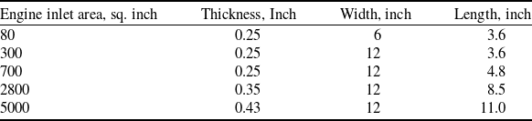
According to the U.S. Federal Aviation Administration (FAA) airworthiness standard ‘14 CFR 33.77 Foreign object ingestion-ice’, the specific requirements for engine ice ingestion testing are outlined, which specify the minimum size of the ice-debris (as shown in Table 3, excerpted [32]). The engine inlet area in this study is 985.8 in2. By interpolation, the minimum size of the ingested ice is calculated to be 0.264 in × 12 in × 5.3 in (equivalent to 6.7 mm × 304.8 mm × 134.6 mm). Based on this minimum size, three factors were considered, leading to the final choice of an ice-debris size of 220 mm × 200 mm × 60 mm:
Minimum ice dimensions based on engine inlet size

-
1. Stokes Number Analysis: The Stokes number compares the inertia of a particle to the characteristic timescale of the flow. According to Equation (12), the Stokes number for the minimum ice-debris size is calculated.
(12)where the ice density is 0.9 g/m3, the characteristic diameter of the ice is computed using the equivalent sphere diameter method as 0.0403 m, the characteristic velocity of fluid is 230 m/s, the dynamic viscosity of the air is 18.6 × 10⁻⁶ Pa·s, and the characteristic fluid length is taken as the inlet equivalent diameter of 0.34 m. Based on this, the Stokes number for the minimum ice size is 2.95 × 10⁶. The high Stokes number: This indicates that the ice-debris has significant inertia, preventing it from closely following the airflow streamlines, which is consistent with real-world observations. Under the same conditions, the selected Stokes number for the ice-debris should be greater than this value. For the chosen ice size, the calculated Stokes number is 1.33 × 10⁷, which preliminarily proves the validity of the ice size choice. However, due to the substantial kinetic energy carried by the high-speed airflow within the inlet duct, the motion of the ice-debris exhibits significant uncertainty, which is dependent on the subsequent velocity and force analyses presented in later sections.
\begin{align}S{\rm{t}} = \frac{{{\tau _p}}}{{{\tau _f}}} = \frac{{{\rho _p}d_p^2U}}{{18\mu {L_f}}},\end{align}
-
2. Limitations of inlet geometry: The high longitudinal offset (0.9 m) and narrow entrance section (with elliptical axes of 0.56 m and 0.28 m) make elongated ice-debris unsuitable for analysis. Such ice is prone to premature wall collisions, which would disrupt the study of its full aerodynamic trajectory. In contrast, the compact dimensions of the selected ice-debris (220 mm × 200 mm × 60 mm) is more stable during motion within the confined and curved duct geometry. They ensure that the debris can effectively traverse the S-shaped path, allowing for meaningful observations and simulations. This choice also reduces the challenges associated with mesh distortion during numerical simulations, making the selected dimensions more practical for studying aerodynamic performance in such duct configurations.
-
3. Characteristics of the external ingestion ice: We referred to the Chinese GJB 5032-2001 regulations for engine hail ingestion tests [Reference Qi, Chang and Yang33]. The standard stipulates the ingestion of one hail particle with a diameter of 5 cm for each 0.25 m² of engine inlet area. Given that the engine inlet area in this study significantly exceeds the reference size, we increased the ice-debris thickness from the baseline 50 mm to 60 mm. This adjustment enables us to simulate a more challenging and realistic ingestion scenario, allowing for the evaluation of the aerodynamic behaviour of ice under demanding conditions.

Overall, the ice-debris with dimensions of 220 mm × 200 mm × 60 mm were selected for simulation as large as possible. The density of the ice is 0.9 g/cm3. The calculated moments of inertia of the ice-debris about each axis are as follows: I xx = 0.010296 kg·m², I yy = 0.017503 kg·m², Izz = 0.008633 kg·m².
3.2.2 Steady-state flow field containing ice
The YF-16 aircraft mentioned uses an F100-PW-229 engine with a rated airflow of 114 kg/s. Instead of the engine operating condition, this paper calculates the flow field by using the negative pressure boundary condition at the outlet of the inlet duct. Based on the above boundary conditions, after establishing the overset mesh, the steady-state flow field when the ice-debris falls at three different positions can be simulated as shown in Fig. 10, which depicts the z = 0 plane of the inlet duct.
Steady-state flow field inside the inlet duct containing delaminating ice.

It can be observed that the airflow velocity is higher at the inlet of the inlet duct in Fig. 10. The high-speed fluid passing through the expansion and transition of the inlet duct causes the airflow velocity to decrease, leading to a tendency towards uniform and stable flow conditions. This can reduce the total-pressure distortion of the high-speed airflow at the engine inlet interface. However, the presence of ice-debris impedes the airflow in the rear region, causing different airflow velocities in the upper and lower parts of the inlet duct. Figure 11 shows the distribution of the total pressure recovery coefficient and streamline at the engine inlet under the three conditions mentioned above. Under the extrusion of the high-speed fluid in the lower part, a pair of inverse vortices is formed due to the change in direction of low kinetic energy fluid in the middle and upper parts, leading to lower total pressure recovery coefficients at corresponding positions. Evidently, as ice-debris approaches the front of the inlet duct, the total pressure recovery coefficient at the engine inlet decreases. It suggests that the ingress of ice-debris at the entrance section leads to a significant airflow loss within the inlet duct, resulting in a notable decline in engine performance. In severe cases, it may induce engine surges or even flameout.
The total-pressure recovery coefficient and streamline of the engine inlet under the three conditions.

3.2.3 Trajectories of ice-debris at different falling positions
The trajectories of ice-debris within the S-shaped inlet were obtained through data analysis and visualisation, as shown in Fig. 12.
The trajectories of ice delaminating at different positions in the inlet duct.

Figure 12(a) reveals that the ice-debris experiences a slight upward motion in the entrance section. It is attributed to the combined effect of airflow and gravity, causing the front part of the ice-debris to tilt upwards and increase the windward area, resulting in a brief upward motion. The vertical velocity variation of the ice-debris, as shown in Fig. 13, clearly illustrates that during the initial stage, the vertical velocity of the ice-debris is positive, reaching a maximum of 1.316 m/s. It indicates that during this stage, the ice-debris experiences a greater lift force from the airflow than gravity. Subsequently, the ice-debris continues to descend under the influence of boundary layer effect at the top of the duct and gravity, ultimately colliding with the bottom wall of the duct. Within the range of 1 m to 2.25 m in the middle section, the velocity variation indicates that the ice-debris experiences an upward force, attributed to the boundary layer effects generated by the bottom wall of the duct.
In the S-shaped and Export sections shown in Fig. 12, the ice-debris is not observed to rise due to the restriction from the top wall of the inlet duct. However, there is a brief transitional period in both sections (as shown in Fig. 13). During this period, the ice-debris experiences a balance between the uplifting force from the airflow and gravity, resulting in a gradual descent with a small velocity. Subsequently, the effect of gravity on the ice-debris becomes significantly stronger, leading to a continuous increase in the downward velocity. Eventually, the ice-debris collides separately with the bottom wall of the duct and the engine fan. To provide detailed information about the motion at the time of collision, the positions and velocities of the ice-debris upon collision are listed in Table 4.
Collision information of delaminating ice at different positions in the inlet duct

The vertical velocity changes of delaminating ice at different positions in the inlet duct.

The comprehensive analysis presented in this section reveals that, besides the aerodynamic influence of high-velocity airflow on the ice-debris, the inlet duct walls and gravity also exert significant effects on the ice behaviour. When the ice is close to the duct walls, the drag or compression generated by the walls prevails over gravity. Conversely, gravity becomes dominant as the ice-debris moves away from the walls. Furthermore, ice-debris falling in the export section has a higher probability of directly impacting the engine fan, posing a greater threat of impact damage to the engine. The ice-debris in the entrance section undergoes greater acceleration from the airflow. Consequently, it exhibits the highest destructive kinetic energy, with the velocity upon collision increasing by 46.51 m/s.
3.3 Effect of different entered attitudes
During aircraft operation, ice-debris formed in snowy weather and ice formed by the condensation of supercooled water inside the inlet duct enter the duct in different ways. Typically, in ground tests, ice-debris formed in snowy weather (hereafter referred to as ingesting ice) is imparted with an initial velocity, while ice formed by supercooled water (hereafter referred to as delaminating ice) enters the duct in free fall. This section first analyses the ingesting ice from the upper, middle and lower regions of the entrance section of the duct, followed by a comparison between ingesting ice taken in from the upper region and delaminating ice. The basic principle for introducing ingesting ice from these three regions is based on reasonable assumptions. Depending on the relative position of the ice-debris to the duct opening, ingesting ice can be captured from three different heights of the intake: the upper, middle and lower regions.
The velocity of the ingested ice is characterised by both its initial speed and inclination angle, with the initial sliding angle set to 45 degrees in this study. The choice of velocity for the ice ingested into the inlet duct differs from that used in engine impact experiments. Excessive velocity would result in immediate contact between the ice and the duct walls, which would not be representative of the aerodynamic behaviour of the ice inside. Authors’ previous simulations indicated that when the vertical velocity exceeds 6 m/s, ice ingested from the lower region of the duct almost instantly collides with the bottom wall. Considering this, a velocity of 6 m/s was chosen for the initial velocity of the external ingested ice in this study. Additionally, in section 3.4, ice ingested from the upper region was tested at velocities of 10 m/s and 13 m/s to investigate the effect of velocity on the aerodynamic behaviour of the ice. Therefore, velocities of 6 m/s and –6 m/s are chosen for the x and y directions, respectively, in this section.
3.3.1 Trajectories of ingesting ice ingested at different positions
Consistent with the flow field calculation method described in the previous section, the airflow rate was adjusted by altering the negative pressure at the outlet of the duct to achieve the rated value of 114 kg/s. The steady-state flow field when ingesting ice just enters the inlet duct is depicted in Fig. 14.
Steady-state flow field of each suction position of ingesting ice.

In comparison to the steady-state flow field of delaminating ice (Fig. 10), the larger windward surface obstructed by the inclined angle of ingesting ice evidently exacerbates the flow losses within the inlet duct. Figure 15 presents the total pressure recovery coefficient and streamline distribution at the engine inlet interface under the three aforementioned conditions. Compared to the case of delaminating ice (Fig. 11), regions with lower total pressure recovery coefficients notably expand, exacerbating the total-pressure distortion at the engine inlet. The cause of lower total pressure recovery coefficients lies in the squeezing action of the bottom high-speed airflow, which alters the direction of the low-speed airflow, thereby generating reverse vortices. Furthermore, the closer the entrance position of the ingesting ice to the upper region, the smaller the total pressure recovery coefficient at the engine inlet. In other words, the higher the ice-debris is positioned, the greater the influence of gas disturbance on the flow losses within the inlet duct.
The trajectories of ice-debris ingesting into the inlet duct from three different positions were obtained through data analysis and visualisation, as shown in Fig. 16. Collision information of ice-debris for the three operating conditions is listed in Table 5.
Collision information of the ice ingesting into the inlet duct at different regions

The total-pressure recovery coefficient and streamline of the engine inlet under the three conditions.

The trajectories of the ice sliding into the inlet duct at different regions.

As shown in Fig. 16, although the intake positions and final landing points of the three types of ice-debris are not consistent, their trajectories are roughly similar. In the initial stage, the ice-debris still moves along the direction of its initial velocity. Subsequently, it experiences a brief upward movement due to the lifting effect of the airflow. Finally, it rapidly descends in the S-shaped section due to the combined effect of the airflow and the squeezing action of the duct walls. Except for the ice taken in from the middle part, all other ice-debris collide with the engine fan face. Furthermore, the velocities of ice at the time of collision under the three operating conditions are 53.17 m/s, 57.37 m/s and 55.10 m/s, respectively, with relatively small differences in kinetic energy carried. However, ice-debris taken in from the upper and lower regions have smaller vertical velocities before collision, which is a key factor leading to their impact on the engine.
The reason for the smaller vertical velocities of ice-debris taken in from the upper and lower region before collision is illustrated in Fig. 17. Within the range of 3 to 3.5m along the x direction (axial direction) of the duct, there exists a ‘Force steering zone’. In this region, the force acting on the ice-debris changes from initially downward to upward vertically. This decelerates the descent velocity of the ice-debris taken in from the upper and lower region, resulting in their vertical velocities being smaller than those taken in from the middle part.
The vertical velocity changes of the ice ingesting into the inlet duct at different parts.

Within the axial range of 3 to 3.5m in the inlet duct, the three types of ice-debris shown in Fig. 18 are positioned near the top wall. However, the forces acting on the ice-debris vary significantly. This phenomenon is not only influenced by wall compression and gravity but also closely related to the orientation of the ice.
The instantaneous state of three kinds of ice in the range of 3 ∼ 3.5 m in the axial direction.

The ice-debris sucked in from the upper and lower regions both form angles greater than 90 degrees with the incoming flow direction (considering upward as the positive direction of the ice-debris), resulting in the formation of a low-pressure separation zone at the upper right part of the ice-debris. In the lower region of ice, under the motion of high-speed airflow, a high-pressure zone is formed, and the significant pressure difference causes the ice to experience an upward lift force. Moreover, as the angle between the ice-debris and the incoming flow direction increases, the pressure difference between its upper and lower surfaces decreases, resulting in less upward lift force acting on the ice. On the contrary, ice-debris ingested from the middle part with an angle less than 90 degrees relative to the incoming flow direction results in a low-pressure separation region located in its lower-right area, inducing a downward force on the ice. By tracking the motion attitudes of three types of ice-debris, it is also evident that this phenomenon applies the entire motion process of ice within the inlet duct. Moreover, the change in the angle between the ice-debris and the incoming flow direction results in the phenomenon of ‘Force steering’.
3.3.2 Trajectories of ice with different attitudes
A comparation of the behaviour of ice-debris with two different attitudes at the upper region of the entrance section was conducted. The trajectory comparison is illustrated in Fig. 19. The trajectories of ice with different attitudes at the upper region of inlet duct, while the vertical velocity is shown in Fig. 20.
The trajectories of ice with different attitudes at the upper region of inlet duct.

The vertical velocity changes of ice with different attitudes at the upper region of inlet duct.

The delaminating ice, lacking an initial velocity, undergoes a slow rise during the initial stage. Subsequently, influenced by gravity and the orientation of the ice-debris, it descends rapidly, ultimately impacting the bottom wall of the inlet duct. In contrast, for ingesting ice, its motion is significantly affected by the orientation of the ice-debris, resulting in a lower descent velocity. Furthermore, the ingesting ice, possessing a horizontal initial velocity aligned with the mainstream direction, induces significant axial displacement. This ultimately leads to an impact on the engine fan face.
The comprehensive comparation reveals that for two different orientations of ice-debris entering the same part of entrance section, the probability of ingesting ice impacting the engine is higher. Moreover, when considering the data presented in Table 4 (Entrance section) and Table 5 (Upper region), ingesting ice also exhibits higher impact kinetic energy.
3.4 Effect of different entered velocities
Taking ingesting ice as the primary focus, a comparative experiment was conducted with velocities of 10 m/s and 13 m/s to investigate the trajectories of ice within the inlet duct at different initial speeds. Through data analysis and visualisation, the trajectories of ingesting ice at three different initial velocities are shown in Fig. 21. It can be observed that the trajectories of ice-debris exhibit obvious regularity, wherein ice-debris with higher initial velocities tend to have lower trajectories and collide with the bottom wall of the duct earlier. The phenomenon is attributed not only to the larger downward displacement of ice-debris with higher initial velocities but also to the orientation of the ice.
The trajectories of ice sliding into the inlet duct at different initial velocities.

It is evident that the ice-debris with an initial velocity of 6 m/s experiences a phenomenon known as ‘force steering’, resulting in a decrease in descent velocity when passing through the S-shaped section. However, ice-debris with initial velocities of 10 m/s and 13 m/s pass through the S-shaped section in a state where the angle with the incoming flow direction is less than 90 degrees. As a result, they experience a downward force from the airflow, accelerating the descent of the ice (as shown in Fig. 22(b)). The horizontal velocity influences the axial displacement of the ice-debris. As shown in Fig. 22(a), the horizontal velocities of the ice increase in all three conditions. However, due to the limited vertical space within the inlet duct, ice-debris with higher vertical velocities tend to impact the duct first, while horizontal velocity does not play a decisive role. Similarly, the velocities of the ice-debris at the time of impact are 53.17 m/s, 55.45 m/s, and 54.56 m/s for the three scenarios respectively, with minor differences in kinetic energy carried (as shown in Table 6). However, ice-debris with smaller initial velocities have a higher probability of impacting the engine.
The collision information of ice ingesting into the inlet at different initial velocities

The velocity changes of ice sliding into the inlet at different initial velocities.

3.5 Effect of different shapes of ice-debris
The shape of the ice significantly influences the aerodynamic forces and moments acting on the object, which in turn affects its interaction with the internal flow field. In the current work, we extended our previous simulations using a cuboid-shaped ice-debris to include two additional shapes: spherical (hail) and irregularly shaped debris. The irregular debris was designed with internal curvature to mimic debris that might break off from the fuselage or wing. In this section, the ice shape [Reference Papadakis, Rachman, Wong, Hung and Bidwell34] was obtained using the NASA Glenn LEWICE ice accretion code with 22.5-minute ice accretion times for the 36-inch chord NACA 23012 aerofoil.
For each shape, we ensured that the total volume remained consistent across all cases, with an initial velocity of 6 m/s for all debris types. The initial position of the debris at the inlet duct entrance was also kept approximately constant to ensure a fair comparison of aerodynamic performance. By conducting simulations on these three types of ice-debris (cuboid, spherical and irregular), we aimed to explore how shape variations influence the aerodynamic forces and trajectories, and consequently, the potential for debris interaction with engine components.
Consistent with the flow field calculation method described in section 3.2.2, the steady-state flow field when ice of different shapes just enters the inlet duct is depicted in Fig. 23.
Steady-state flow field and pressure recovery inside the inlet duct containing different shape of ice.

As shown in Fig. 23, under three conditions, the tilted cuboid and irregular ice-debris cause strong flow separation and turbulence near the ice due to their sharp edges. This affects the airflow downstream of the inlet duct, resulting in lower total-pressure recovery coefficients in the lower regions of the duct outlet, which is disadvantageous for engine intake performance. In contrast, the spherical ice generates less disturbance, which is primarily concentrated in the central region of the inlet duct. The airflow remains relatively stable, leading to lower energy losses in the inlet duct. Overall, non-streamlined ice-debris cause more significant disturbances to the airflow, severely reducing the airflow recovery efficiency at the engine intake.
Through data analysis and visualisation, the trajectories of different shapes of ingesting ice inside the inlet duct are shown in Fig. 24.
It can be observed that the trajectories of the different ice shapes do not exhibit significant regularity. Specifically, the spherical ice undergoes an initial descent, then nearly moves horizontally before colliding with the S-bend section of the duct. The cuboid and irregular ice show similar trajectories, both of which ultimately collide with the engine fan.
Unlike the previous case, spherical ice does not experience the ‘Force steering’ phenomenon due to its shape. As it descends, the closer the spherical ice approaches the lower wall of the duct, the stronger the aerodynamic lift, eventually reaching a near force equilibrium and causing horizontal motion. The variation in vertical velocity shown in Fig. 25(b) explains this phenomenon, with minimal and nearly constant vertical force in the later stages of the ice’s movement. Figure 25(b) also shows that the force distribution in irregularly ice is more complex than in cubic ice, with multiple small fluctuations. When areas with larger curvatures face the oncoming airflow, the flow pattern around the ice changes, leading to a transient increase or decrease in lift. Additionally, curvature variations can cause flow separation in localised regions, forming vortical structures that contribute to vertical lift fluctuations. Of course, the above conclusions also apply to explaining the fluctuations in horizontal velocity of the irregular ice (as shown in Fig. 25(a)).
The collision information of different shapes of ingesting ice inside the inlet duct

The trajectories of different shapes of ingesting ice inside the inlet duct.

The velocity changes of different shapes of ingesting ice inside the inlet duct.

Table 7 presents the collision data for different shapes of ice within the inlet duct. The spherical ice, due to its early collision with the duct wall, experienced a smaller increase in velocity. Moreover, as a result of the rotational effects, irregular and cuboid ice are more likely to undergo spinning or irregular tumbling during their movement, resulting in a higher rate of horizontal velocity increase compared to spherical ice under similar conditions (Fig. 25(a)). Ultimately, the irregularly ice exhibits the highest destructive kinetic energy, with a velocity increase approaching six times the initial value.
4.0 conclusion
A Euler-Lagrange two-phase flow model was designed and established to analyse the motion of ice-debris in the dorsal S-shaped inlet. With the prerequisite of obtaining a stable flow field containing ice-debris, the 6-DOF overset mesh technique was employed to address the motion of ice-debris in the high-speed flow field within the inlet duct. Furthermore, the numerical model’s high accuracy was validated through similar experimental data. Key information regarding the trajectory, attitude, collision velocity and collision position of ice-debris in the dorsal S-shaped inlet under different parameters was obtained. The summarised patterns provide valuable data references for optimising complex inlet ducts of aircraft and studying foreign object damage in subsequent research.
-
1. The ingestion of ice-debris, especially non-streamlined shapes like cuboid and irregular debris, significantly exacerbates total-pressure distortion at the engine inlet by causing greater flow disturbance and reducing intake performance. Moreover, the closer the ice-debris is to the upper region of the inlet duct’s entrance section, the greater the flow loss within the inlet duct, leading to poorer aerodynamic performance of the engine.
-
2. In addition to the influence of gravity and wall’s boundary layer effects, the orientation of the ice-debris relative to the incoming flow direction is a decisive factor in its force dynamics. When the angle between the ice and the incoming flow direction exceeds 90 degrees (considering upward as the positive direction of the ice), the ice experiences an upward force, with a smaller angle resulting in less upward force. Conversely, the angles below 90 degrees induce a downward force, accelerating its descent.
-
3. Ice-debris has a higher probability of impacting the engine when it falls from the export section of the inlet duct, posing a greater threat of impact damage to the engine. In contrast, ice-debris detached from the entrance section experiences a stronger acceleration effect from the airflow, with a velocity increment of up to 46.51 m/s, resulting in higher kinetic energy upon impact with the walls of the inlet duct.
-
4. For ice ingested from different positions, the velocity amplification before collision can exceed 520%. Irregularly ice, due to rotational effects, exhibits a velocity increase of up to six times and generates higher destructive kinetic energy. Moreover, ice-debris ingested from both the upper and lower regions of the entrance section have a higher probability of impacting the engine fan. Additionally, ice-debris with smaller initial velocities have a greater probability of impacting the engine, with larger velocity amplifications.
Acknowledgments
This project was supported by the Fundamental Research Funds for the Central Universities (N2025013) and the National Natural Science Foundation of China (Grant No. 51934002).
Competing interests
No conflict of interest exists in the submission of this manuscript, and manuscript is approved by all authors for publication.
Appendix: Code for solving diffuser shape parameters
import numpy as np
from scipy.integrate import quad
from scipy.optimize import fsolve, root
def integrand(y, n):
return (1 - y* *n)* *(1/n)
def objective_function(n, x, L, M, D, K, dy):
y = dy * (3 * (x/L)* *4 - 8 * (x/L)* *3 + 6 * (x/L)* *2)
J = (np.pi * M * M) / K
C = np.pi * M * M
U = D * np.sqrt(J / (np.pi * D))
V = np.sqrt(J / (np.pi * D))
S = 0.25 * J * (((C/J - 1) * (3 * (x/L)* *4 - 8 * (x/L)* *3 + 6 * (x/L)* *2)) + 1)
a = np.sqrt((M* *2 - U* *2) * (3 * (x/L)* *4 - 8 * (x/L)* *3 + 6 * (x/L)* *2) + U* *2)
b = np.sqrt((M* *2 - V* *2) * (3 * (x/L)* *4 - 8 * (x/L)* *3 + 6 * (x/L)* *2) + V* *2)
if not hasattr(objective_function, "already_printed"):
print("S: {:.5f}".format(S*4))
print("a: {:.5f}".format(a))
print("b: {:.5f}".format(b))
objective_function.already_printed = True
result, _ = quad(lambda y: integrand(y, n), 0, 1)
return result - S / (a * b)
initial_guess = 1
# parameters setting
K_val = * * * # diffusion ratio
M_val = * * * # outlet radius, m
D_val = * * * # aspect ratio of elliptical inlet
L_val = * * * # diffuser length, m
dy_val = * * * # longitudinal offset, m
x_val = * * * # x-direction position, m
numerical_solution_fsolve, info_fsolve, ier, msg = fsolve(objective_function, initial_guess, args=(x_val, L_val, M_val, D_val, K_val, dy_val), full_output=True)
numerical_solution_root = root(objective_function, initial_guess, args=(x_val, L_val, M_val, D_val, K_val, dy_val), method=‘hybr’)
tolerance = 0.000000001
if np.abs(numerical_solution_fsolve[0] - numerical_solution_root.x[0]) < tolerance:
final_result = (numerical_solution_fsolve[0] + numerical_solution_root.x[0]) / 2
print("The iterative solution of n is: {:.5f}".format(final_result))
else:
print("error!")