1 Introduction
The performance and pollutant emission of combustion devices heavily depend on the evaporation and homogeneity of the fuel–air mixture which is controlled by the preceding atomization process. It describes the disintegration of a liquid core into a large number of droplets. Further crucial technical applications can be found in medicine (e.g. asthma spray) or agriculture (e.g. manuring apparatus). The underlying physics of spray formation, especially the interaction between the turbulent flow and the liquid–gas interface, is not yet fully understood (Desjardins et al. Reference Desjardins, McCaslin, Owkes and Brady2013).
The development of advanced numerical techniques in the context of direct numerical simulation (DNS) significantly improved our understanding of the atomization physics. Each exhibiting particular advantages and disadvantages, the volume-of-fluid method (Hirt & Nichols Reference Hirt and Nichols1981), the level-set method (Sussman, Smereka & Osher Reference Sussman, Smereka and Osher1994) and the front-tracking method (Tryggvason et al. Reference Tryggvason, Bunner, Esmaeeli, Juric, Al-Rawahi, Tauber, Han, Nas and Jan2001) are well established for accurate interface propagation. One of the first reported diesel spray DNS at low Reynolds and Weber number goes back to Leboissetier & Zaleski (Reference Leboissetier and Zaleski2001), demonstrating that no break-up occurs for laminar flow conditions inside the nozzle. Taking into account realistic turbulent conditions at the injection nozzle, DNS of a liquid sheet exhausting into gaseous atmosphere was performed by Klein (Reference Klein2005). For the planar water jet at the low Weber number of 270, no jet break-up and spray formation occurred. Flow and interface statistics in the near-nozzle region were also compared to experimental data, revealing good qualitative agreement. Sander & Weigand (Reference Sander and Weigand2008) later found that not only the inflow turbulence characteristics but also the mean velocity profile at the inlet has a strong influence on the stability of liquid sheets. Accompanied by a first discussion of mesh resolution requirements in the context of two-phase DNS, diesel jet simulations at an increased Weber number of 11 600, showing severe liquid break-up, were presented by Ménard, Tanguy & Berlemont (Reference Ménard, Tanguy and Berlemont2007). This discussion of resolution requirements for the smallest interfacial structures was continued by Desjardins & Pitsch (Reference Desjardins and Pitsch2010) who studied the break-up of a temporally evolving turbulent liquid sheet at Weber numbers between 500 and 2000. Herrmann (Reference Herrmann2011) investigated the primary atomization of a round diesel jet, also highlighting the impact of finite grid resolution on interface geometry and droplet size distributions. Highly resolved round diesel jets at the high Weber number of 14 000, injected at laminar conditions into stagnant air, were presented by Shinjo & Umemura (Reference Shinjo and Umemura2010).
To obtain a comprehensive picture of the jet atomization phenomenon, this paper contributes with a local flow topology analysis based on the invariants of the velocity-gradient tensor following the pioneering work of Perry & Chong (Reference Perry and Chong1987) and Chong, Perry & Cantwell (Reference Chong, Perry and Cantwell1990). In the case of incompressible flows, all possible small-scale flow structures can be categorized into two nodal and two focal topologies. To analyse the different manifestations of coherent structures, the methodology has been applied to a variety of flows including wall-bounded shear flows (Chong et al. Reference Chong, Soria, Perry, Chacin, Cantwell and Na1998) and homogeneous isotropic turbulence (Elsinga & Marusic Reference Elsinga and Marusic2010). In the context of incompressible two-phase flows, Hasslberger, Klein & Chakraborty (Reference Hasslberger, Klein and Chakraborty2018b ) analysed the distribution of local flow topologies in bubbly air–water systems. It has been found that focal topologies, representing vortical motion, predominantly reside inside the gaseous bubbles. An example of application to a single-phase jet flow has been presented by Watanabe et al. (Reference Watanabe, Sakai, Nagata, Ito and Hayase2014) who focused upon vortex stretching and compression near the turbulent/non-turbulent interface in a planar jet. The authors are not aware of any applications of this methodology to liquid jet atomization however. If the flow is compressible, e.g. in the context of turbulent premixed combustion (Wacks et al. Reference Wacks, Chakraborty, Klein, Arias and Im2016), the first invariant (trace) of the velocity-gradient tensor assumes non-zero values. The number of possible flow topologies consequently increases from four to eight. Potential further analysis steps were demonstrated by Dopazo, Martín & Hierro (Reference Dopazo, Martín and Hierro2007) who studied the connection between local flow topologies and local interface curvature. Including also the evolution of the invariants, an extension of the snapshot-based topology analysis has been proposed by Ooi et al. (Reference Ooi, Martin, Soria and Chong1999).
2 Direct numerical simulation database
2.1 Numerical methodology
The state-of-the-art two-phase solver PARIS (PArallel Robust Interface Simulator, written in Fortran, and developed by Stéphane Zaleski et al. at Institut Jean Le Rond d’Alembert, UPMC & CNRS, Paris, France; see Ling, Zaleski & Scardovelli Reference Ling, Zaleski and Scardovelli2015) was applied for the simulations discussed in this paper. This code is based on the one-fluid formulation of the unsteady incompressible Navier–Stokes equations including capillary forces. Two immiscible fluids are represented by a jump in density and viscosity. Propagation of the phase interface is implicitly calculated by an advection equation
 $$\begin{eqnarray}\frac{\unicode[STIX]{x2202}\unicode[STIX]{x1D6FC}}{\unicode[STIX]{x2202}t}+u_{j}\frac{\unicode[STIX]{x2202}\unicode[STIX]{x1D6FC}}{\unicode[STIX]{x2202}x_{j}}=0\end{eqnarray}$$
for the cell-based volume fraction
 $\unicode[STIX]{x1D6FC}$
of the liquid phase. Cell-averaged fluid properties are then obtained from a weighted arithmetic mean for density and dynamic viscosity,
 $$\begin{eqnarray}\displaystyle & \displaystyle \unicode[STIX]{x1D70C}=\unicode[STIX]{x1D6FC}\unicode[STIX]{x1D70C}_{l}+(1-\unicode[STIX]{x1D6FC})\unicode[STIX]{x1D70C}_{g}, & \displaystyle\end{eqnarray}$$
 $$\begin{eqnarray}\displaystyle & \displaystyle \unicode[STIX]{x1D707}=\unicode[STIX]{x1D6FC}\unicode[STIX]{x1D707}_{l}+(1-\unicode[STIX]{x1D6FC})\unicode[STIX]{x1D707}_{g}. & \displaystyle\end{eqnarray}$$
The subscripts
 $g$
and
 $l$
indicate the gaseous and liquid phase, respectively. To obtain the velocity field
 $\boldsymbol{u}$
, the momentum balance equation for two-phase flows
 $$\begin{eqnarray}\unicode[STIX]{x1D70C}\left(\frac{\unicode[STIX]{x2202}u_{i}}{\unicode[STIX]{x2202}t}+\frac{\unicode[STIX]{x2202}u_{i}u_{j}}{\unicode[STIX]{x2202}x_{j}}\right)=-\frac{\unicode[STIX]{x2202}p}{\unicode[STIX]{x2202}x_{i}}+\frac{\unicode[STIX]{x2202}\unicode[STIX]{x1D70F}_{ij}}{\unicode[STIX]{x2202}x_{j}}+\unicode[STIX]{x1D70E}\unicode[STIX]{x1D705}n_{i}\unicode[STIX]{x1D6FF}_{S}\end{eqnarray}$$
is solved, in which the interface Dirac function
 $\unicode[STIX]{x1D6FF}_{S}\equiv \unicode[STIX]{x1D6FF}(\boldsymbol{x}-\boldsymbol{x}_{S})$
is approximated by
 $|\unicode[STIX]{x1D735}\unicode[STIX]{x1D6FC}|$
, and thus
 $\boldsymbol{n}\unicode[STIX]{x1D6FF}_{S}=-\unicode[STIX]{x1D735}\unicode[STIX]{x1D6FC}$
, according to the continuum surface force methodology proposed by Brackbill, Kothe & Zemach (Reference Brackbill, Kothe and Zemach1992). The quantities
 $\unicode[STIX]{x1D70E}$
,
 $\unicode[STIX]{x1D705}$
and
 $\boldsymbol{n}=-\unicode[STIX]{x1D735}\unicode[STIX]{x1D6FC}/|\unicode[STIX]{x1D735}\unicode[STIX]{x1D6FC}|$
denote the surface tension, interface mean curvature and interface-normal vector, respectively. The viscous stress tensor
 $\unicode[STIX]{x1D70F}_{ij}$
is formulated on the basis of Stokes’ hypothesis, which reduces to
 $$\begin{eqnarray}\unicode[STIX]{x1D70F}_{ij}=\unicode[STIX]{x1D707}\left(\frac{\unicode[STIX]{x2202}u_{i}}{\unicode[STIX]{x2202}x_{j}}+\frac{\unicode[STIX]{x2202}u_{j}}{\unicode[STIX]{x2202}x_{i}}\right)\end{eqnarray}$$
for incompressible flows (
 $\unicode[STIX]{x1D735}\boldsymbol{\cdot }\boldsymbol{u}=0$
).
In terms of interface treatment, advanced numerical techniques are applied: a geometrical volume-of-fluid method including piecewise linear interface reconstruction, and a height function method combined with continuous surface force balancing for interface curvature determination (Popinet Reference Popinet2018). In the framework of the finite-volume method, spatial discretization on a cubic staggered grid is implemented by the third-order quadratic upstream interpolation for convective kinematics (QUICK) scheme for momentum advection and the second-order central differencing scheme for diffusive fluxes. Volume fraction advection, equation (2.1), is implemented by the calcul d’interface affine par morceaux (CIAM) scheme (Scardovelli & Zaleski Reference Scardovelli and Zaleski2003) (similar to the method of Parker & Youngs (Reference Parker and Youngs1992)) and explicit temporal discretization by a second-order accurate Runge–Kutta scheme. The projection method invokes a successive over-relaxation solver for the pressure Poisson equation. Parallelization is realized by the domain decomposition technique and MPI processor communication. Further details on the utilized numerical techniques can be found in Tryggvason, Scardovelli & Zaleski (Reference Tryggvason, Scardovelli and Zaleski2011).
2.2 Computational set-up
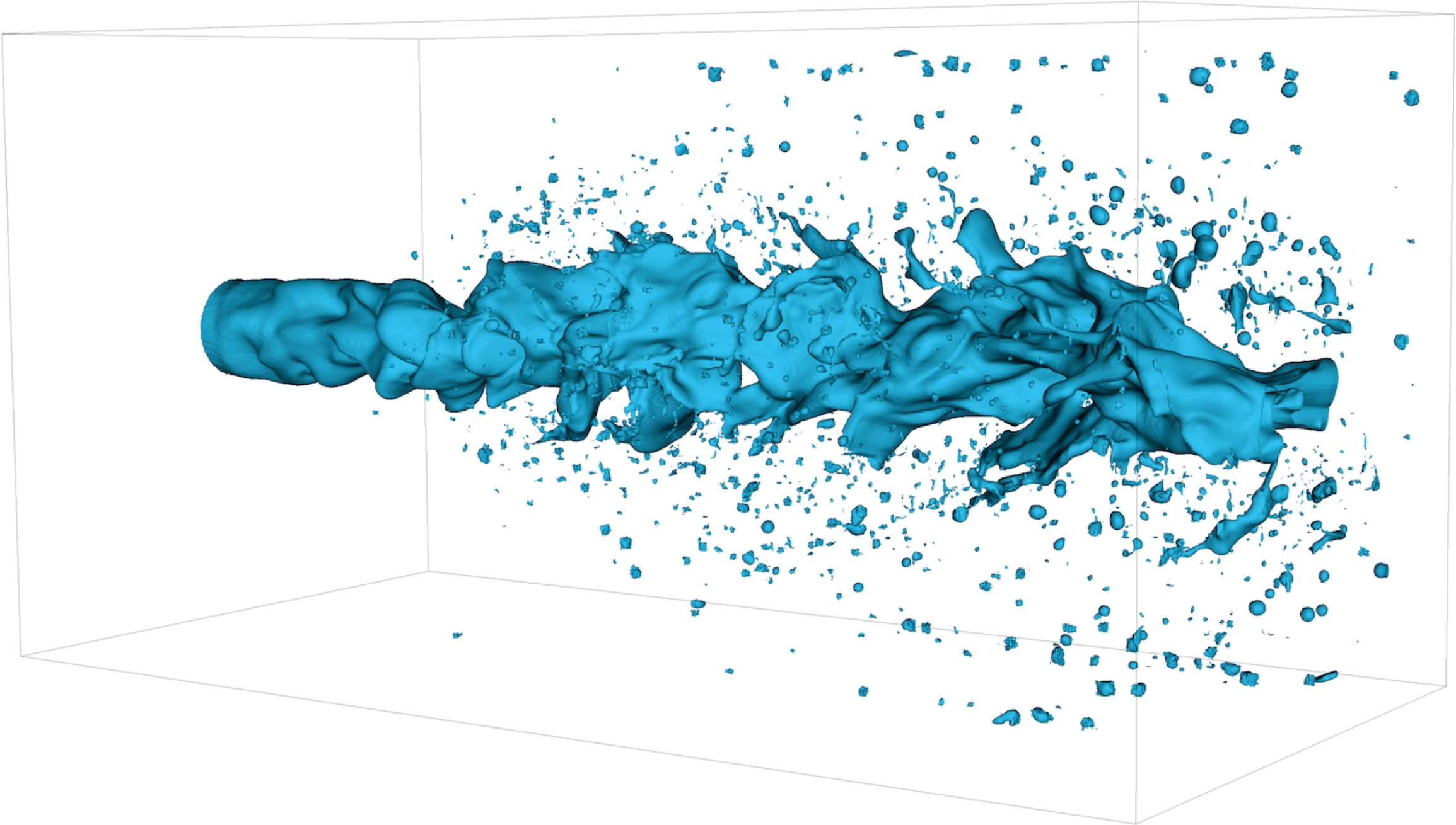
Three-dimensional round jet configuration: primary atomization in the hi
 $Re$
-lo
 $We$
case visualized by the blue
 $\unicode[STIX]{x1D6FC}=0.5$
iso-contour indicating the liquid–gas interface. The mean flow direction is oriented from left to right.

The investigated set-up is similar to the configuration studied by Ketterl & Klein (Reference Ketterl and Klein2018). For one of the examined cases, figure 1 visualizes the primary atomization process. The liquid is injected through a round nozzle on the left and the interface immediately starts to wrinkle according to the turbulent inflow conditions. Interface corrugations grow in the downstream direction and ligaments are formed. These ligaments are stretched, eventually rupture and form droplets. Secondary atomization, i.e. the break-up of droplets into smaller droplets, is naturally included in the simulation but is not at the focus of this work.
The near field of a liquid round jet injected through a nozzle into a quiescent gas is a classical flow instability problem. Mean vorticity and its fluctuations evolve from a wall-confined stream to an unbound environment as the flow leaves the nozzle. Coherent structures (Brown & Roshko Reference Brown and Roshko1974), due to the mean vorticity shedding, form, grow and interact with vorticity fluctuations downstream of the nozzle. For large enough Reynolds numbers, the flow transitions to a turbulent jet. Due to the liquid jet oscillation and due to the no-slip condition at the liquid–gas interface, pressure and viscous forces set the initially quiescent gas in motion.
The rectangular computational domain extends
 $12D$
in the axial direction and
 $6D$
in both spanwise directions, where
 $D$
denotes the diameter of the round nozzle. At the side boundaries, homogeneous Neumann conditions are imposed, including a narrow band where the velocity is filtered to avoid numerical instabilities. At the outflow boundary, back-flow into the domain is prevented by clipping negative velocities to zero, also for stability reasons. Dirichlet conditions are applied at the inlet boundary. To imitate a turbulent channel flow inside the nozzle region, the mean velocity profile of Stanley, Sarkar & Mellado (Reference Stanley, Sarkar and Mellado2002) is superimposed by a homogeneous isotropic fluctuation level of 5 % and an integral turbulent length scale of
 $L_{t}=D/4$
using the digital filter method of Klein, Sadiki & Janicka (Reference Klein, Sadiki and Janicka2003). This method is based on the scaling and Gaussian filtering of random fluctuations, and it reproduces first- and second-order one-point statistics as well as given length scales.
Corresponding to diesel engine conditions at a pressure of approximately 5.2 MPa and a temperature of approximately 900 K, the density and viscosity ratio are specified to be
 $\unicode[STIX]{x1D70C}_{l}/\unicode[STIX]{x1D70C}_{g}=40$
and
 $\unicode[STIX]{x1D707}_{l}/\unicode[STIX]{x1D707}_{g}=40$
, respectively. It follows that there is no jump of kinematic viscosity at the phase boundary, i.e.
 $\unicode[STIX]{x1D708}=\unicode[STIX]{x1D708}_{l}=\unicode[STIX]{x1D708}_{g}$
. The liquid viscosity
 $\unicode[STIX]{x1D707}_{l}$
and the surface tension
 $\unicode[STIX]{x1D70E}$
are adjusted to achieve the desired values of the inflow-based Reynolds number
 $Re=\unicode[STIX]{x1D70C}_{l}u_{0}D/\unicode[STIX]{x1D707}_{l}$
and Weber number
 $\mathit{We}=\unicode[STIX]{x1D70C}_{l}u_{0}^{2}D/\unicode[STIX]{x1D70E}$
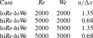
in table 1, respectively.
Spatial discretization by a uniform Cartesian mesh of grid size
 $\unicode[STIX]{x0394}x=\unicode[STIX]{x0394}y=\unicode[STIX]{x0394}z=D/64$
yields an overall number of
 $768\times 384\times 384\approx 1.13\times 10^{8}$
computational cells. According to the universal equilibrium theory by Kolmogorov, the smallest dissipative length scale that has to be resolved for DNS can be estimated by
 $\unicode[STIX]{x1D702}\sim L_{t}Re_{t}^{-3/4}$
using the integral turbulent length scale
 $L_{t}$
and the turbulent Reynolds number
 $Re_{t}=u^{\prime }L_{t}/\unicode[STIX]{x1D708}_{l}$
(Batchelor Reference Batchelor1953). Inserting the prescribed inflow characteristics for
 $u^{\prime }$
and
 $L_{t}$
yields
 $\unicode[STIX]{x1D702}/\unicode[STIX]{x0394}x$
values between 0.68 and 1.35: cf. table 1. Thus, the grid size is of the order of the Kolmogorov length scale in all investigated cases, and should be sufficient to resolve small-scale flow topologies. It is hardly possible to draw further conclusions from the given values of
 $\unicode[STIX]{x1D702}/\unicode[STIX]{x0394}x$
because their calculation is based on dimensional considerations rather than being exact.
Case overview in terms of the inflow-based Reynolds number
 $Re$
, Weber number
 $\mathit{We}$
and estimated ratio of Kolmogorov length scale to grid spacing
 $\unicode[STIX]{x1D702}/\unicode[STIX]{x0394}x$
.

Manual mesh refinement (in one coordinate direction) is not a convenient choice because the interface is moving heavily, showing arbitrary alignment with the underlying mesh and including strong topological changes. Alternative strategies like adaptive mesh refinement involve new issues like flux splitting at the boundary between different refinement levels as well as load balancing in a massively parallel environment. Furthermore, the theoretical order of discretization is difficult to maintain for local mesh refinement. The usage of uniform meshes is a standard procedure for solvers, which are based on a geometrical volume-of-fluid method since this method provides some kind of sub-grid treatment of the interface (Ménard et al. Reference Ménard, Tanguy and Berlemont2007; Ling et al. Reference Ling, Fuster, Zaleski and Tryggvason2017). There are further practical aspects related to the meshing strategy. The implementation of special-purpose post-processing tools (like the topology analysis in this work) is relatively straightforward for uniform Cartesian meshes. Any kind of interpolation introduces a new source of uncertainty.
Resolution of the Kolmogorov scale might not be sufficient in the context of two-phase flow DNS simulations. Turbulent structures are believed to follow cascade dynamics such that the smallest flow structures can be determined based on dimensional arguments. However, primary atomization is a more complex problem. In particular, the stretching and break-up of thin ligament structures is a highly nonlinear process involving strong topological changes, and does not necessarily follow a cascade process (Ling et al. Reference Ling, Zaleski and Scardovelli2015). It is a matter of ongoing discussion how to determine the required mesh density in terms of accurate representation of interface dynamics. There are empirical criteria (e.g. by Desjardins & Pitsch Reference Desjardins and Pitsch2010) to evaluate the grid spacing with respect to droplet stability resolution requirements. Nevertheless, a universal criterion, e.g. based on dimensional arguments, has not been found so far. Furthermore, the required resolution always depends on the kind of information to be extracted from the simulation. First- and second-order statistics like mean flow and fluctuation profiles converge faster than higher-order statistics. For very sensitive statistics like droplet size distributions, it may even be impossible to achieve a grid-independent solution, as argued by Herrmann (Reference Herrmann2011) and Ling et al. (Reference Ling, Fuster, Zaleski and Tryggvason2017).
The same point in time is compared for all four cases. Considering the constant time step
 $\unicode[STIX]{x0394}t$
, which yields a Courant–Friedrichs–Lewy (CFL) number of approximately 0.3, the analysed snapshot after 15 000
 $\unicode[STIX]{x0394}t$
corresponds to approximately 3.5 flow-through times based on the centreline velocity.
3 Mathematical background
According to Perry & Chong (Reference Perry and Chong1987) and Chong et al. (Reference Chong, Perry and Cantwell1990), amongst others, the invariants of the velocity-gradient tensor
 $$\begin{eqnarray}\unicode[STIX]{x1D608}_{ij}\equiv \frac{\unicode[STIX]{x2202}u_{i}}{\unicode[STIX]{x2202}x_{j}}=\unicode[STIX]{x1D61A}_{ij}+\unicode[STIX]{x1D61E}_{ij}\end{eqnarray}$$
give rise to a set of local flow topologies. Here,
 $\unicode[STIX]{x1D61A}_{ij}=0.5(\unicode[STIX]{x1D608}_{ij}+\unicode[STIX]{x1D608}_{ji})$
and
 $\unicode[STIX]{x1D61E}_{ij}=0.5(\unicode[STIX]{x1D608}_{ij}-\unicode[STIX]{x1D608}_{ji})$
represent the tensor’s symmetric and anti-symmetric components, respectively. The corresponding characteristic equation
 $\unicode[STIX]{x1D706}^{3}+P\unicode[STIX]{x1D706}^{2}+Q\unicode[STIX]{x1D706}+R=0$
exhibits three solutions, i.e. the eigenvalues
 $\unicode[STIX]{x1D706}_{1}$
,
 $\unicode[STIX]{x1D706}_{2}$
and
 $\unicode[STIX]{x1D706}_{3}$
of
 $\unicode[STIX]{x1D608}_{ij}$
. Since the first invariant of
 $\unicode[STIX]{x1D608}_{ij}$
is given by
 $$\begin{eqnarray}P\equiv -\text{trace}(\unicode[STIX]{x1D608}_{ij})=-(\unicode[STIX]{x1D706}_{1}+\unicode[STIX]{x1D706}_{2}+\unicode[STIX]{x1D706}_{3})=-S_{ii}=0\end{eqnarray}$$
for incompressible flows (
 $\unicode[STIX]{x1D735}\boldsymbol{\cdot }\boldsymbol{u}=0$
), the second and third invariant of
 $\unicode[STIX]{x1D608}_{ij}$
reduce to
 $$\begin{eqnarray}Q\equiv (\text{trace}(\unicode[STIX]{x1D608}_{ij})^{2}-\text{trace}(\unicode[STIX]{x1D608}_{ij}^{2}))/2=(-\unicode[STIX]{x1D61A}_{ij}\unicode[STIX]{x1D61A}_{ij}+\unicode[STIX]{x1D61E}_{ij}\unicode[STIX]{x1D61E}_{ij})/2\end{eqnarray}$$
and
 $$\begin{eqnarray}R\equiv -\text{det}(\unicode[STIX]{x1D608}_{ij})=(-\unicode[STIX]{x1D61A}_{ij}\unicode[STIX]{x1D61A}_{jk}\unicode[STIX]{x1D61A}_{ki}-3\unicode[STIX]{x1D61E}_{ij}\unicode[STIX]{x1D61E}_{jk}\unicode[STIX]{x1D61A}_{ki})/3.\end{eqnarray}$$
The characteristic equation’s discriminant
 $$\begin{eqnarray}D=(27R^{2}+4Q^{3})/108\end{eqnarray}$$
divides the
 $Q{-}R$
phase space into two regions:
 $D>0$
, where
 $\unicode[STIX]{x1D608}_{ij}$
shows one real eigenvalue and two complex conjugate eigenvalues (and therefore focal topologies), and
 $D<0$
, where
 $\unicode[STIX]{x1D608}_{ij}$
shows three real eigenvalues (and therefore nodal topologies). Corresponding to
 $D=0$
, two lines separating the topologies in the phase space are given by
 $$\begin{eqnarray}\displaystyle & \displaystyle r_{1a}=-2(-3Q)^{3/2}/27, & \displaystyle\end{eqnarray}$$
 $$\begin{eqnarray}\displaystyle & \displaystyle r_{1b}=+2(-3Q)^{3/2}/27. & \displaystyle\end{eqnarray}$$
In the region
 $D>0$
,
 $\unicode[STIX]{x1D608}_{ij}$
has purely imaginary eigenvalues on the line
 $r_{2}=0$
. The lines
 $r_{1a}$
,
 $r_{1b}$
and
 $r_{2}$
divide the
 $Q{-}R$
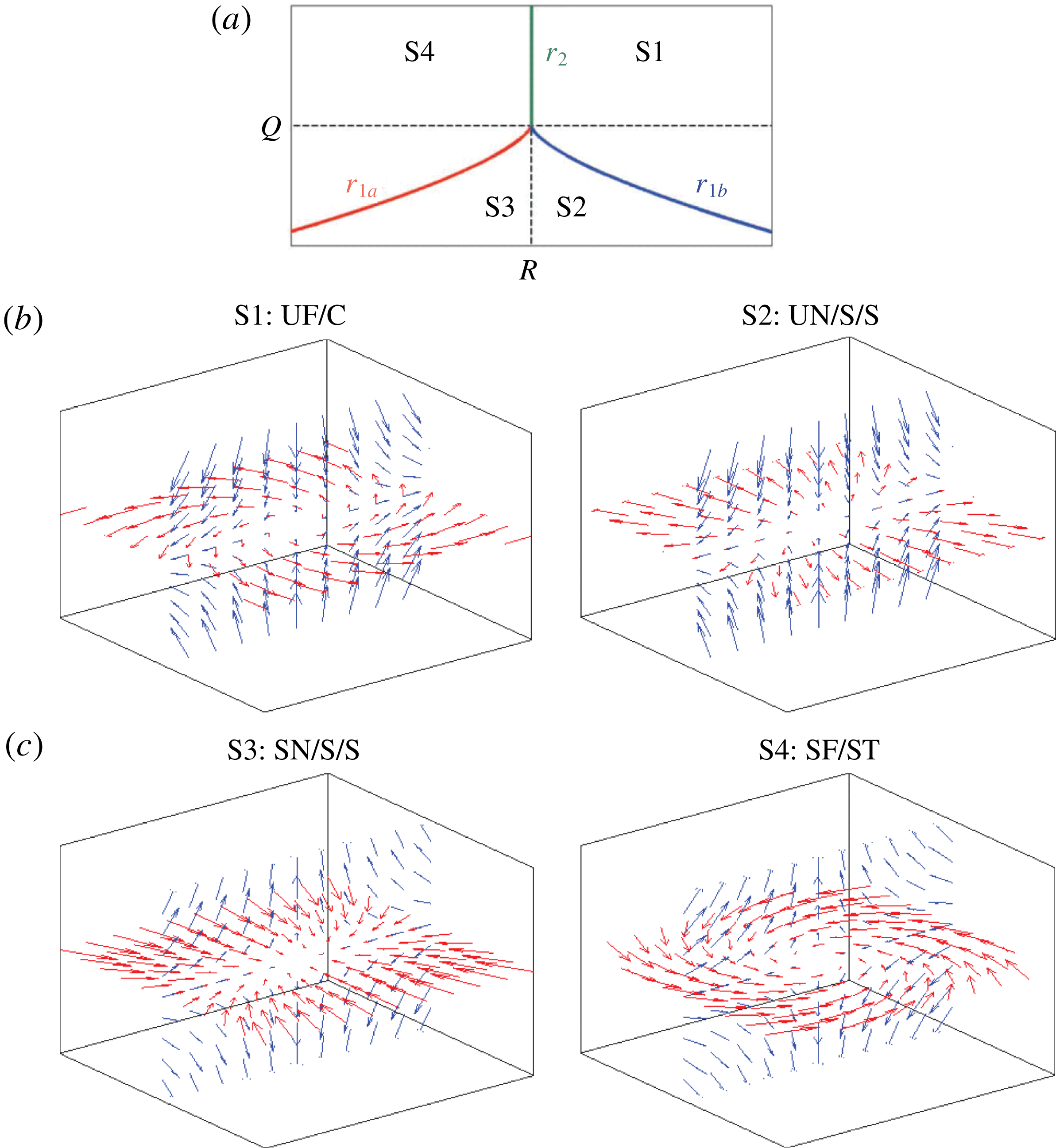
phase space into four flow topologies in the incompressible case. Both the topology borders
 $r_{1a}$
,
 $r_{1b}$
and
 $r_{2}$
in the
 $Q{-}R$
phase space, as well as a graphical representation of topologies S1–S4, are shown in figure 2. To simplify the interpretation, the second invariant of
 $\unicode[STIX]{x1D608}_{ij}$
,
 $Q$
, can be split into two parts:
 $$\begin{eqnarray}Q=Q_{S}+Q_{W}=-\unicode[STIX]{x1D61A}_{ij}\unicode[STIX]{x1D61A}_{ij}/2+\unicode[STIX]{x1D61E}_{ij}\unicode[STIX]{x1D61E}_{ij}/2,\end{eqnarray}$$
where
 $Q_{S}$
and
 $Q_{W}$
denote the second invariants of
 $\unicode[STIX]{x1D61A}_{ij}$
and
 $\unicode[STIX]{x1D61E}_{ij}$
, respectively.
 $Q_{S}$
is always a negative quantity since
 $-4\unicode[STIX]{x1D708}Q_{S}=2\unicode[STIX]{x1D708}\unicode[STIX]{x1D61A}_{ij}\unicode[STIX]{x1D61A}_{ij}$
, i.e. the dissipation of kinetic energy into heat per unit mass. The latter part
 $Q_{W}$
is directly related to vorticity
 $\unicode[STIX]{x1D74E}$
and enstrophy
 $\unicode[STIX]{x1D6F7}$
according to
 $$\begin{eqnarray}\unicode[STIX]{x1D61E}_{ij}\unicode[STIX]{x1D61E}_{ij}/2=\unicode[STIX]{x1D714}_{i}\unicode[STIX]{x1D714}_{i}/4=\unicode[STIX]{x1D6F7}/2.\end{eqnarray}$$
Thus,
 $Q<0$
is indicative of strain-dominated regions and
 $Q>0$
is indicative of vorticity-dominated regions.
(a) Classification of topologies S1–S4: projection of topology borders
 $r_{1a}$
,
 $r_{1b}$
and
 $r_{2}$
in the
 $Q{-}R$
plane. Dashed lines indicate
 $Q=0$
and
 $R=0$
, respectively. (b,c) Graphical representation corresponding to UF
 $=$
unstable focus, UN
 $=$
unstable node, SN
 $=$
stable node, SF
 $=$
stable focus, C
 $=$
compressing, S
 $=$
saddle, ST
 $=$
stretching.

4 Results and discussion
4.1 Vorticity field
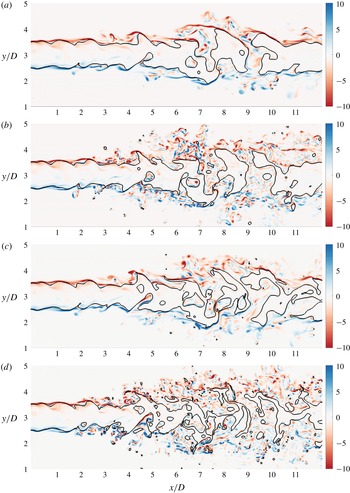
Since vortical motion is inherently connected to the nature of turbulence, a first impression of the atomization flow dynamics is given by means of the plane-normal component of the vorticity, i.e.
 $\unicode[STIX]{x1D714}_{z}=\unicode[STIX]{x2202}u_{y}/\unicode[STIX]{x2202}x-\unicode[STIX]{x2202}u_{x}/\unicode[STIX]{x2202}y$
in figure 3 and
 $\unicode[STIX]{x1D714}_{x}=\unicode[STIX]{x2202}u_{z}/\unicode[STIX]{x2202}y-\unicode[STIX]{x2202}u_{y}/\unicode[STIX]{x2202}z$
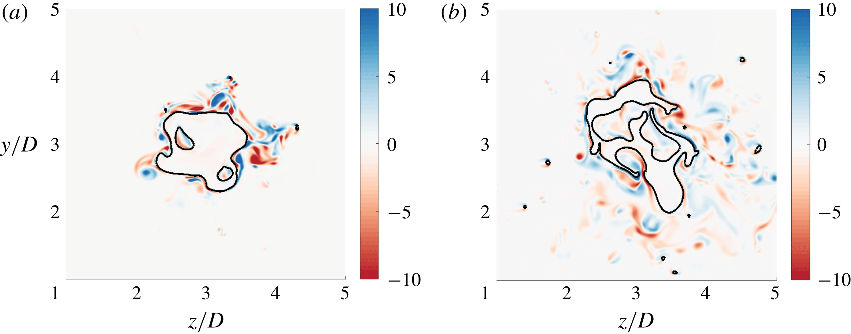
in figure 4. The slices in figure 4 represent two different stages of the jet break-up process. The vorticity and topology distributions are obviously strongly linked as elaborated in § 3. Some aspects of the flow are similar in all four cases.
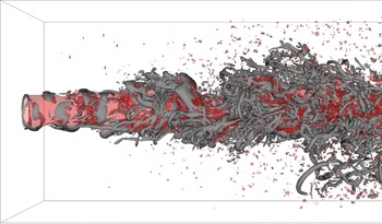
Counter-rotating vortex pairs can wrinkle and pinch off liquid structures. However, separated liquid structures can induce vortex pairs in a similar manner. Both phenomena can be identified in figure 3. The causality is not unambiguous in this context. Besides, it is difficult to draw consistent conclusions from two-dimensional slices since the considered structures, e.g. thin ligaments, do not necessarily align with the observation plane. In general, the liquid structures exhibit a strongly three-dimensional shape. Lasheras & Choi (Reference Lasheras and Choi1988) experimentally showed that streamwise and spanwise vortices are interacting and leading to a three-dimensional turbulent planar mixing layer. In the round jet configuration investigated here, azimuthal (i.e. vortex rings) and axial vorticity components are interacting as is evident from figure 5. Since the behaviour is qualitatively in agreement with the other cases, only the lo
 $Re$
-hi
 $We$
case is shown. In order to accentuate dominant focal structures (referring to topology S1 or S4), the three-dimensional
 $Q=5u_{0}^{2}/D^{2}$
iso-contour is displayed. In the high Reynolds number cases, the focal structures are even smaller and harder to distinguish.
Slices of the normalized plane-normal component of vorticity
 $\unicode[STIX]{x1D714}_{z}D/u_{0}$
, with the black line indicating the phase interface. From (a) to (d): lo
 $Re$
-lo
 $We$
, hi
 $Re$
-lo
 $We$
, lo
 $Re$
-hi
 $We$
, hi
 $Re$
-hi
 $We$
.

The lo
 $Re$
-hi
 $We$
case: slices of the normalized plane-normal component of vorticity
 $\unicode[STIX]{x1D714}_{x}D/u_{0}$
, with the black line indicating the phase interface, for two different axial locations:
 $x/D=4$
(a) and
 $x/D=8$
(b).

The lo
 $Re$
-hi
 $We$
case: three-dimensional iso-contours of
 $\unicode[STIX]{x1D6FC}=0.5$
(semi-transparent red) indicating the phase interface and
 $Q=5u_{0}^{2}/D^{2}$
(grey) indicating dominant focal structures.

Moreover, noticeable vorticity production occurs in the shear layers close to the inlet, where the jet is still compact. It is well known that vorticity is produced in shear layers (Brown & Roshko Reference Brown and Roshko1974). This is exactly the situation in the vicinity of the nozzle where a strong vertical gradient of axial velocity,
 $\unicode[STIX]{x2202}u_{x}/\unicode[STIX]{x2202}y$
, can be found. In this region, the gas is initially at rest whereas the liquid velocity is still close to the inlet velocity. As can be seen, the sign of the induced vorticity is reversed on opposite sides of the jet. This observation might be interpreted as vortices wrapping around the liquid jet.
The vorticity level in the liquid phase is clearly lower than in the gaseous phase, which is characterized by a lower density but also lower viscosity. Tripathi, Sahu & Govindarajan (Reference Tripathi, Sahu and Govindarajan2014) claim that vorticity accumulates in the lighter fluid independent of the viscosity ratio and the concaveness/convexness of the interface which follows from stability arguments (Dixit & Govindarajan Reference Dixit and Govindarajan2010). In order to exclude the viscosity ratio being responsible for this behaviour, Tripathi et al. (Reference Tripathi, Sahu and Govindarajan2014) imposed identical viscosities in their simulation and observed the same behaviour. Dopazo, Lozano & Barreras (Reference Dopazo, Lozano and Barreras2000) present an analytically exact instantaneous relation between the vorticity values immediately above and below the interface, as a function of the strain-rate tensor components and the viscosity ratio. However, using a linearized prediction equally applicable to the vorticity values immediately above and below the interface, Farsoiya, Mayya & Dasgupta (Reference Farsoiya, Mayya and Dasgupta2017) found that the vorticity jump across the interface generally depends on both the density and viscosity ratio of the two fluids. Both statements from the literature do not contradict an additional vorticity accumulation effect due to density differences, in unsteady turbulent flows and in regions sufficiently away from the interface.
The jet half-width (radial distance at which the considered variable drops to 50 % of the corresponding mean centreline value) with respect to the velocity field is clearly larger than with respect to the liquid volume fraction.
As a first approximation, the effects of the variation of Reynolds and Weber number (cf. table 1) on jet break-up seem to be comparable in the sense of the intact liquid core length and the number of separated ligaments or droplets. Strongest break-up consequently appears in the high Reynolds high Weber case. Increasing the Weber number means that the effect of surface tension forces is reduced compared to inertia effects. Accordingly, interfacial structures are less rounded off and tend to develop thin ligaments with sharp edges. This behaviour can also be observed in figure 3. In contrast, the size of turbulent flow structures in the gaseous phase is determined by the Reynolds number. According to the common understanding, smaller structures are expected at higher values of the Reynolds number. This behaviour is not directly evident since the enhanced jet break-up might induce additional turbulent motion in the gaseous phase.
4.2 Topology field
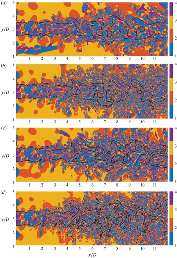
Figure 6 shows the result of the invariants-based topology analysis introduced in § 3. The topology field, consisting of focal topologies S1 (blue) and S4 (purple) as well as nodal topologies S2 (red) and S3 (orange), confirms the impression from the vorticity field that the size of flow structures is mainly determined by the Reynolds number. Agreeing with the cascade process in turbulent flows, a spectrum of topology island sizes can be observed, which will be quantified in § 4.4. It should be kept in mind that the kinematic viscosity
 $\unicode[STIX]{x1D708}$
and therefore the Reynolds number based on inflow conditions,
 $Re=u_{0}D/\unicode[STIX]{x1D708}$
, is identical in both phases. However, the turbulent Reynolds number
 $Re_{t}=u^{\prime }L_{t}/\unicode[STIX]{x1D708}$
varies locally and appears to be higher in the gaseous phase. Examining DNS statistics of a three-dimensional two-phase jet configuration at a similar inflow-based Reynolds number (Klein Reference Klein2005), it may roughly be estimated that
 $u_{l}^{\prime }/u_{g}^{\prime }\approx 0.2$
and
 $L_{t,l}/L_{t,g}\approx 0.5$
. Accordingly,
 $Re_{t,l}/Re_{t,g}\approx 0.1$
– a difference of approximately one order of magnitude in terms of the turbulent Reynolds number.
Another interesting observation from figure 6 is the periodic occurrence of nodal S2 structures near the points of maximum local interface deflection on the gas side in the vicinity of the interface near the nozzle. In an independent study on the topology distribution in incompressible bubbly flows, Hasslberger, Klein & Chakraborty (Reference Hasslberger, Klein and Chakraborty2018a ) and Hasslberger et al. (Reference Hasslberger, Klein and Chakraborty2018b ) observed a switch from nodal topology S2 to nodal topology S3 when the character of the flow around the bubble changes from diverging (up to the bubble centre) to converging (behind the bubble centre), respectively. In both the case from the literature and the case investigated here, the switch of nodal topology occurs at the position of maximum local interface deflection.
The liquid flow structures in the vicinity of the inlet nozzle are similar in all cases since the synthetic turbulent inflow velocity and the analysed time snapshot are identical. The focal topologies at the left boundary, outside of the nozzle region, must be assessed as spurious behaviour which stems from the ill-conditioned velocity-gradient tensor in that region. This nearly laminar flow region is in fact a correct solution of the Navier–Stokes equations, i.e. the flow solution itself does not show any spuriousness. Since the topology classification is local, spurious identification in some regions does not affect the results in the rest of the computational domain. Provided that the velocity gradients are non-zero (satisfied everywhere except in the mentioned region), the topology classification is correct.
Slices of the flow topology field where 1–4 in the colour bar refer to S1–S4 respectively; the black line indicates the phase interface. From (a) to (d): lo
 $Re$
-lo
 $We$
, hi
 $Re$
-lo
 $We$
, lo
 $Re$
-hi
 $We$
, hi
 $Re$
-hi
 $We$
.

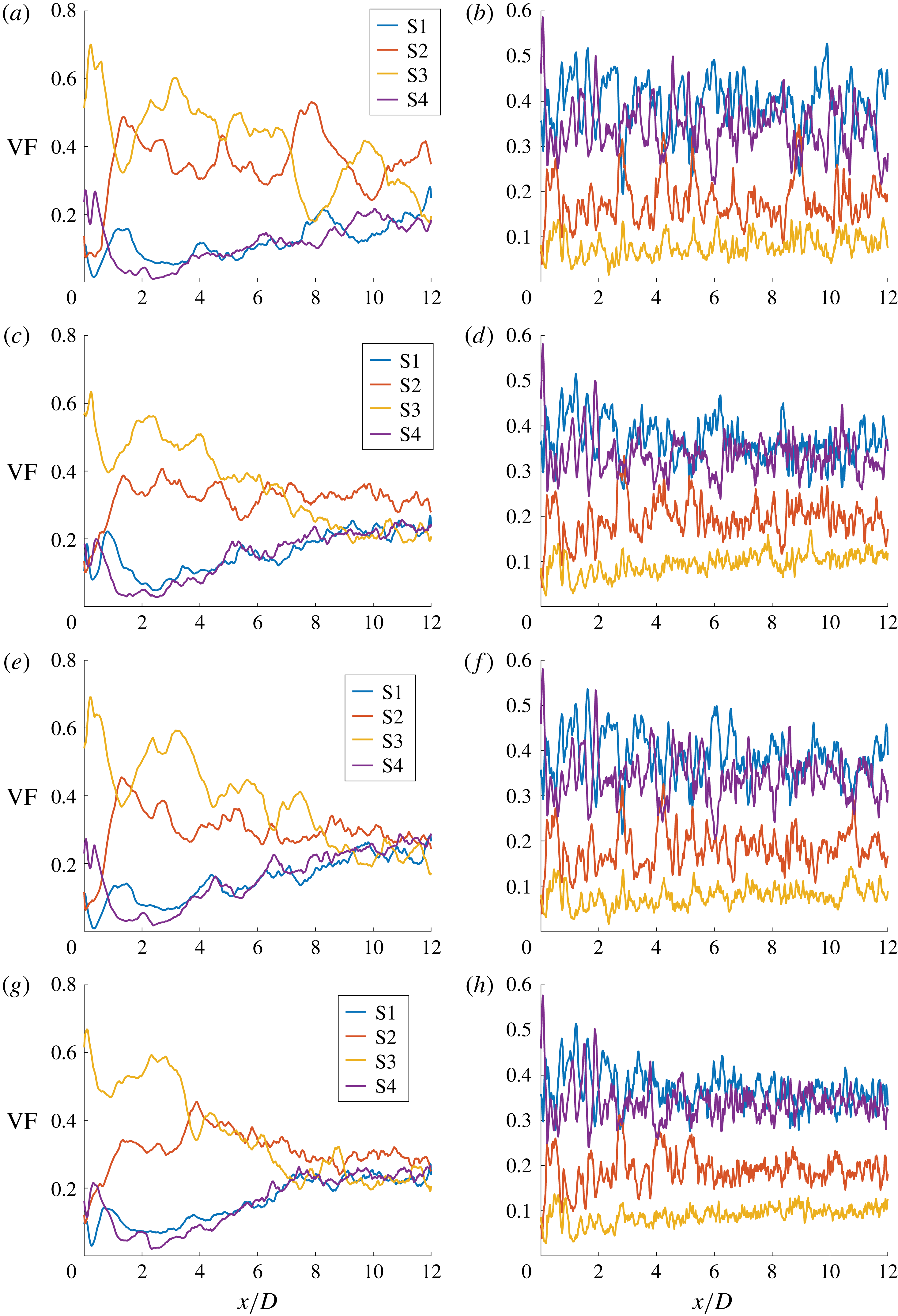
Axial volume fraction distribution of focal topologies S1 and S4 as well as nodal topologies S2 and S3 for the gaseous phase (a,c,e,g) and liquid phase (b,d,f,h). From top to bottom: lo
 $Re$
-lo
 $We$
, hi
 $Re$
-lo
 $We$
, lo
 $Re$
-hi
 $We$
, hi
 $Re$
-hi
 $We$
.

4.3 Axial volume fraction distribution
The axial development of plane-averaged (with respect to both spanwise directions) topology volume fractions is depicted in figure 7. The data are evaluated in a conditional manner, i.e. separately for the gaseous phase (a,c,e,g) and the liquid phase (b,d,f,h). In the gaseous phase, from inlet to outlet, the share of focal topologies S1 and S4 increases at the expense of nodal topologies S2 and S3 as vortical motion is continuously induced by the mechanisms mentioned in § 2.2. It is worth noting that a coupling of azimuthal and axial vorticity filaments, as displayed in figure 5, is involved in the nodal-to-focal transition process in the axial direction. Whereas the general behaviour is the same in all cases, the tendency towards an asymptotic state with respect to the volume fraction distribution scales both with
 $Re$
and
 $\mathit{We}$
. As discussed above, the size of the topology islands scales primarily with
 $Re$
but the corresponding averaged volume fractions seem to depend also on
 $\mathit{We}$
. Regarding the global exchange from nodal topology S3 to nodal topology S2 in the axial direction, the gas entrainment from the surrounding atmosphere of the jet must be taken into account. There is a net inflow via the side boundaries of the domain which, for small values of
 $x/D$
, gives rise to a globally converging flow situation in the gaseous phase (corresponding to S3). The entrainment increases in the axial direction (note that there is a no-slip condition at the inflow plane everywhere except the nozzle) and saturates roughly where the liquid jet starts breaking up, at around
 $x/D=5$
. The inward-directed radial flow at the lateral boundaries is countered by the break-up and spreading of the jet flow, resulting in local diverging flow situations surrounding the liquid core (corresponding to S2). Figure 6 shows that the major part of the converging S3 topologies can be found at the lateral boundaries towards the nozzle side, whereas the diverging S2 topologies are mainly found at the edge of the developing and expanding shear flow. Accordingly, the dominant nodal topology changes from S3 to S2 at a certain distance from the nozzle. In the investigated set-up, the cross-over point occurs approximately at half of the axial domain length but the location generally depends on the size of the computational domain in the radial direction. Nevertheless, the physical processes are unaffected by the domain set-up.
In the liquid phase, only marginal changes in the axial direction can be observed. Due to the fluctuating nature of the two-phase jet flow, the topology shares are oscillating but their means remain at a fairly constant level. Note that the behaviour directly at the nozzle is prescribed by the synthetic turbulent inflow data. In all cases, the volume fraction is at approximately 35 % for focal topologies S1 and S4, somewhat below 20 % for nodal topology S2 and approximately 10 % for nodal topology S3.
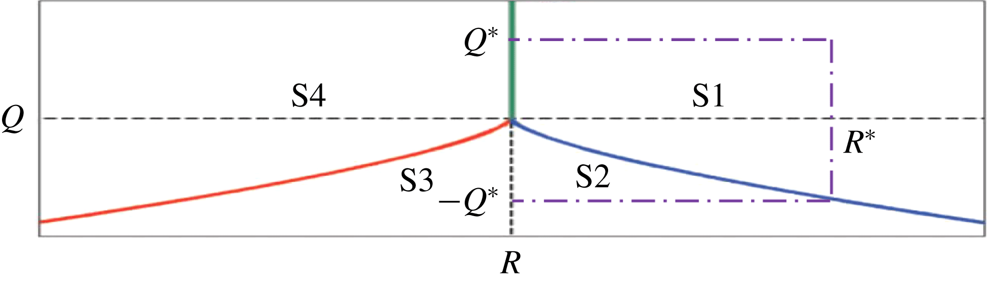
Incompressible topology map including the topology borders
 $r_{1a}$
(red line),
 $r_{1b}$
(blue line),
 $r_{2}$
(green line) and the hypothetical boundary between populated and unpopulated regions (dash-dotted purple line). Dashed black lines indicate
 $Q=0$
and
 $R=0$
, respectively.

The following theoretical discussion on incompressible homogeneous isotropic turbulence serves as a reference for comparison. The topology border relationship
 $$\begin{eqnarray}r_{1b}(Q)\propto (-3Q)^{3/2}\end{eqnarray}$$
reflects the scaling behaviour of the second and third invariant: cf. § 3.
 $Q(C\cdot \unicode[STIX]{x1D608}_{ij})=C^{2}\cdot Q(\unicode[STIX]{x1D608}_{ij})$
and
 $R(C\cdot \unicode[STIX]{x1D608}_{ij})=C^{3}\cdot R(\unicode[STIX]{x1D608}_{ij})$
hold for any arbitrary constant
 $C\in \text{I\!R}^{+}$
since
 $\text{trace}(C\cdot \unicode[STIX]{x1D608}_{ij})=C\cdot \text{trace}(\unicode[STIX]{x1D608}_{ij})$
and
 $\det (C\cdot \unicode[STIX]{x1D608}_{ij})=C^{3}\cdot \det (\unicode[STIX]{x1D608}_{ij})$
. In other words, scaling of a reference flow solution to obtain different levels of velocity fluctuation
 $u^{\prime }$
or integral length scale
 $L_{t}$
does not change the classification of each sample in the topology diagram. The corner point (
 $Q^{\ast },R^{\ast }$
) of a hypothetical rectangle, which is lying on the mentioned topology border (cf. figure 8), is given by
 $$\begin{eqnarray}R^{\ast }=r_{1b}(Q=Q^{\ast })=2/27(-3Q^{\ast })^{3/2}.\end{eqnarray}$$
Let us now assume that the rectangle represents the boundary between heavily populated (towards the origin) and poorly populated (towards infinity) regions in the topology diagram. In realistic flows, local deviations from the rectangular shape are likely to exist but may well annihilate each other in terms of the populated area. The populated area
 $\unicode[STIX]{x1D6FA}_{S2}$
corresponding to topology S2 can then be calculated by
 $$\begin{eqnarray}\unicode[STIX]{x1D6FA}_{S2}=\left|\int _{0}^{Q^{\ast }}r_{1b}(Q)\,\text{d}Q\right|=4/405(-3Q^{\ast })^{5/2}.\end{eqnarray}$$
The assumption of a homogeneous isotropic flow suggests a symmetric population in the
 $Q{-}R$
space such that the populated overall area
 $\unicode[STIX]{x1D6FA}$
reads
 $$\begin{eqnarray}\unicode[STIX]{x1D6FA}=\mathop{\sum }_{k=1}^{4}\unicode[STIX]{x1D6FA}_{Sk}=2Q^{\ast }\cdot 2R^{\ast }.\end{eqnarray}$$
The presented ansatz finally allows for the calculation of the different volume fractions,
 $$\begin{eqnarray}\displaystyle & \displaystyle \text{VF}_{S2}=\text{VF}_{S3}=\unicode[STIX]{x1D6FA}_{S2}/\unicode[STIX]{x1D6FA}=10\,\%, & \displaystyle\end{eqnarray}$$
 $$\begin{eqnarray}\displaystyle & \displaystyle \text{VF}_{S1}=\text{VF}_{S4}=(\unicode[STIX]{x1D6FA}/2-\unicode[STIX]{x1D6FA}_{S2})/\unicode[STIX]{x1D6FA}=40\,\%, & \displaystyle\end{eqnarray}$$
which are independent of the particular choice of
 $Q^{\ast }$
(and therefore
 $R^{\ast }$
). Thus, the total percentage of volume fractions in incompressible homogeneous isotropic turbulence is expected to be 20 % for nodal and 80 % for focal topologies. The two-phase jet configuration investigated here naturally deviates from this idealized state. In particular, the nodal topology S2 is increased (at the expense of other topologies), which matches the globally diverging character of the jet flow.
4.4 Topology island size distribution
For example, in spray combustion, the investigation of turbulence–chemistry interaction is an outstanding field of research. In this context, it is important to know the spectrum of turbulent length scales interacting with the flame. A flood-fill algorithm is thus applied here to determine the size distribution of the topology islands. Regarding the connectivity definition of discrete topology fields, three possibilities naturally arise. Eventually, the usage of face neighbours (6 potential neighbours of each cell not residing at the domain boundary) was preferred over edge neighbours (18 potential neighbours) and point neighbours (26 potential neighbours). Especially when using point neighbours, a disproportionately strong neighbourhood connectivity was observed. Owing to the exponential character of the size distribution, the size range is partitioned into 50 exponentially sized bins. At the lowest level, the island size is limited to three finite-volume cells to exclude single- and double-cell islands which are likely to be influenced by numerical effects.
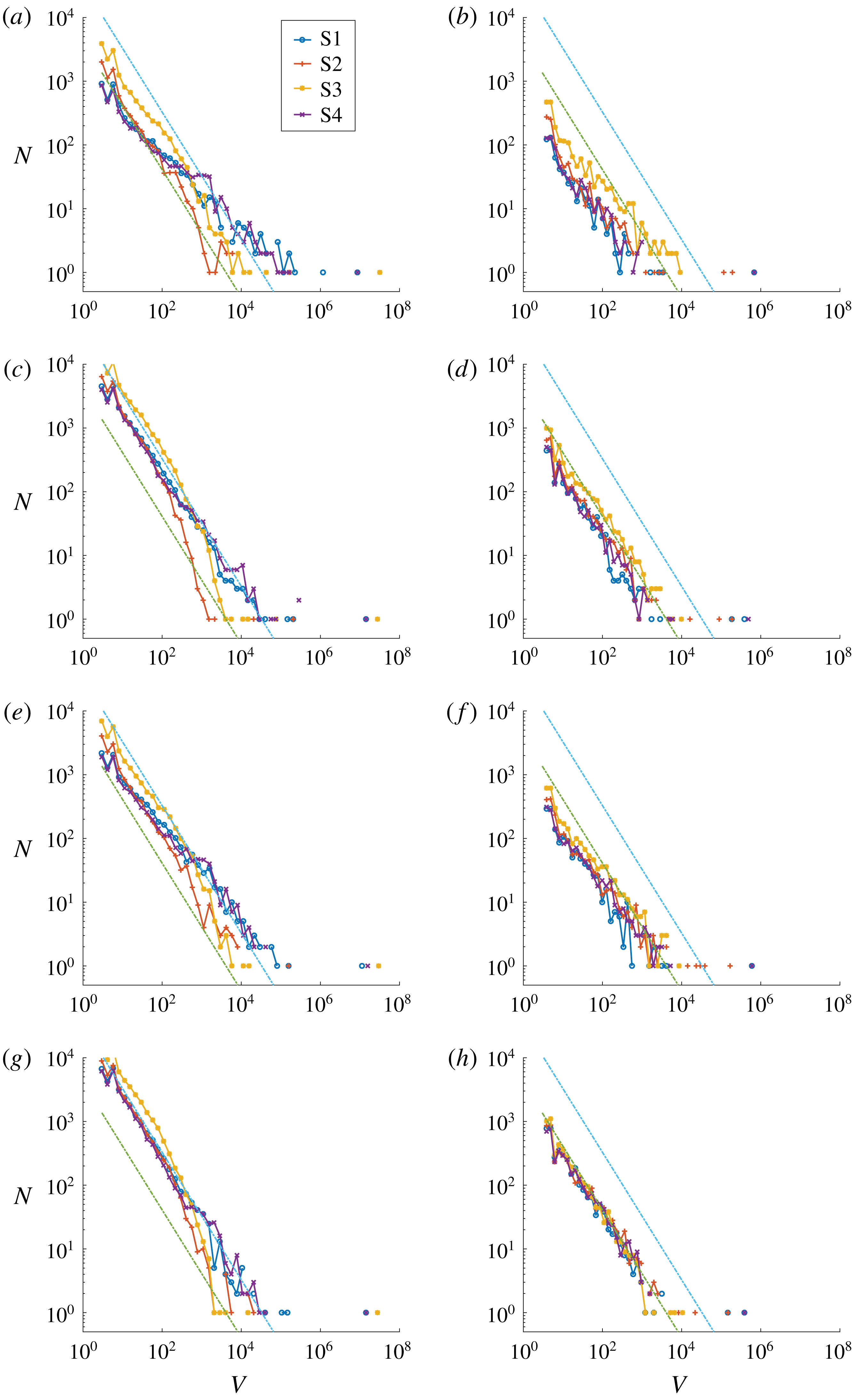
Topology island size distribution for the gaseous phase (a,c,e,g) and liquid phase (b,d,f,h). The turquoise and the green line represent the corresponding power law models of the gaseous phase and the liquid phase, respectively. From top to bottom: lo
 $Re$
-lo
 $We$
, hi
 $Re$
-lo
 $We$
, lo
 $Re$
-hi
 $We$
, hi
 $Re$
-hi
 $We$
.

Inspecting the result in figure 9, where
 $N$
is the number of topology islands of a certain size
 $V=V^{\ast }/(\unicode[STIX]{x0394}x)^{3}$
where
 $V^{\ast }$
is the actual topology island volume, several interesting observations can be made: most prominently, the size distribution follows roughly a linear trend in the log–log diagram for all four cases and it appears to be consistently higher in the gaseous phase (a,c,e,g) than in the liquid phase (b,d,f,h). Outliers, not following the linear trend, occur scarcely at large island sizes for all cases and are mainly located in the laminar region, i.e. sufficiently away from the jet core. In the less homogeneous gaseous phase, the linear trend is slightly less pronounced and small differences between nodal and focal topologies can be identified. Furthermore, the number of nodal topologies S3 for small island sizes is slightly increased compared to the other topologies – an observation that has also been made in turbulent premixed combustion (Chakraborty et al.
Reference Chakraborty, Wacks, Ketterl, Klein and Im2018).
The approximately linear size distribution in the log–log diagram suggests a power law formulation to describe the topology spectrum. Its derivation is based on the general ansatz
 $$\begin{eqnarray}N(V)=aV^{b}\end{eqnarray}$$
with the constants
 $a,b\in \text{I\!R}$
. First of all, we require
 $$\begin{eqnarray}\int _{V_{min}}^{V_{max}}N(V)\,\text{d}V=\text{VF}_{Sk}\cdot V_{total},\end{eqnarray}$$
where
 $\text{VF}_{Sk}$
is the volume fraction of the considered topology
 $\text{S}k$
(
 $k\in [1,2,3,4]$
). It follows that
 $$\begin{eqnarray}\frac{a}{b+1}\left(V_{max}^{b+1}-V_{min}^{b+1}\right)=\text{VF}_{Sk}\cdot V_{total}\end{eqnarray}$$
for
 $b\neq -1$
. For
 $b=-1$
,
 $\ln (V)$
appears as the primitive. Considering the scale disparity in turbulent flows, it is reasonable to assume
 $|V_{max}^{b+1}|\gg |V_{min}^{b+1}|$
and therefore
 $$\begin{eqnarray}\frac{a}{b+1}V_{max}^{b+1}\approx \text{VF}_{Sk}\cdot V_{total}.\end{eqnarray}$$
Now, let us assume we have
 $\unicode[STIX]{x1D713}\in \text{I\!N}$
structures of size
 $V_{max}$
:
 $$\begin{eqnarray}N(V=V_{max})=aV_{max}^{b}=\unicode[STIX]{x1D713}.\end{eqnarray}$$
Inserting (4.11) into (4.10) to eliminate
 $a$
yields
 $$\begin{eqnarray}b\approx \frac{\unicode[STIX]{x1D713}V_{max}}{\text{VF}_{Sk}\cdot V_{total}}-1.\end{eqnarray}$$
Using
 $\text{VF}_{Sk}\cdot V_{total}\gg \unicode[STIX]{x1D713}V_{max}$
, we finally obtain
 $b\approx -1$
and hence
 $a\approx V_{max}\unicode[STIX]{x1D713}$
.
Alternatively, one may interpret
 $V$
as the actual topology island volume and the power law
 $N(V)=aV^{b}$
as the corresponding number density. It is then clear from dimensional arguments that
 $b=-1$
.
To obtain a useful simple model of the spectrum, we require
 $$\begin{eqnarray}N(V=V_{max})=1\end{eqnarray}$$
which is equivalent to setting
 $\unicode[STIX]{x1D713}=1$
. The topology size distribution then reads
 $$\begin{eqnarray}N(V)=V_{max}V^{-1}\end{eqnarray}$$
and
 $V_{max}=(L_{t}/\unicode[STIX]{x0394}x)^{3}$
is taken to be the corresponding volume measure of the integral turbulent length scale
 $L_{t}$
. As can be seen in figure 9, there may exist a few larger topology islands (usually at occurrence one) but the number
 $N$
does not considerably increase above the volume corresponding to
 $L_{t}$
. We know
 $L_{t,l}\approx D/4$
from the prescribed inflow data and we re-use
 $L_{t,l}/L_{t,g}\approx 50\,\%$
from § 4.2 to obtain
 $L_{t,g}\approx D/2$
. Both models for the gaseous phase (turquoise line) and liquid phase (green line) are included in figure 9. Since
 $\text{VF}_{Sk}$
does not enter the simple model, it does not distinguish between different topologies. Consequently, the model is identical for all four cases, only distinguishing the gaseous and liquid phases. In a general situation,
 $L_{t}$
may be estimated by the nozzle diameter
 $D$
as a first-order approximation.
It has been seen in § 4.2 that the topology field is determined by the Reynolds number rather than the Weber number. Since the total turbulent volume
 $V_{total}$
(i.e. the region where both focal and nodal topologies appear; somewhat larger than the spray volume) is smaller in the low Reynolds cases,
 $b>-1$
must be expected in these cases according to (4.12). From a close examination of figure 9, the slightly different slope in the log–log diagram can be discerned because of the aforementioned effect.
The convincing performance of this simple model raises the question whether this method can be used to estimate the integral length scale
 $L_{t}$
when this quantity is a priori unknown in complex flows. There is some algorithmic complexity involved to determine the topology size distribution but its advantage lies in the fact that it is based on a single time snapshot (which is usually available, in contrast to long time series). Following the standard procedure,
 $L_{t}$
is obtained by the integration of the normalized auto-correlation tensor which requires a certain, sometimes considerable, length of the time series to guarantee a reasonable result. The proposed methodology might be seen as an alternative to the well-established approximation
 $L_{t}\approx k^{3/2}/\unicode[STIX]{x1D716}$
(where
 $\unicode[STIX]{x1D716}$
is the dissipation rate of the specific turbulent kinetic energy
 $k$
), which requires statistics as well.
5 Concluding remarks
Using a direct numerical simulation database of primary jet atomization, a local flow topology analysis has been performed based on the invariants of the velocity-gradient tensor. It categorizes all possible small-scale flow structures into two focal and two nodal topologies for incompressible flows.
Although both the inflow-based Reynolds number and Weber number are heavily influencing the jet break-up, the flow topology behaviour seems rather to be dominated by the Reynolds number. As may be expected, the flow dynamics in the gaseous phase is generally less homogeneous than in the liquid phase because some flow regions resemble a laminar-to-turbulent transition state rather than fully developed turbulence. Regarding the axial development of topology volume fractions, a strong shift from nodal to focal topologies was observed in the gaseous phase. In the liquid phase, the topology shares remain fairly constant in the axial direction (fluctuations due to the oscillating jet behaviour excluded).
The discussion of DNS observations is complemented by a theoretical derivation of topology volume fractions in incompressible homogeneous isotropic turbulence. This reference solution allows for the comparison with atomization cases which only slightly deviate from this idealized state in the liquid phase. Additionally, a simple model of the size distribution of flow structures is proposed. Motivated by the approximately linear behaviour of the topology spectrum in the log–log diagram, a power law ansatz is adopted. The only other input to the model is the turbulent integral length scale which is assumed to be different in both phases. Applying reverse logic, it may be possible to utilize the snapshot-based topology analysis to estimate the integral turbulent length scale when this quantity is a priori unknown in complex flows. The robustness of this hypothesis is however yet to be assessed for a broader range of flow conditions.
Future work deals with the development of sub-grid models for the computationally more efficient large eddy simulation. Observations from the topology analysis, e.g. the ratio of focal to nodal topologies, might be helpful to derive appropriate assumptions in the context of functional or structural modelling of interface-dominated two-phase flows.
Acknowledgements
Support by the German Research Foundation (Deutsche Forschungsgemeinschaft – DFG, GS: KL1456/1-1 and KL1456/4-1) is gratefully acknowledged. Computer resources for this project have been provided by the Gauss Centre for Supercomputing/Leibniz Supercomputing Centre under grant no. pr48no. The authors also express their gratitude to the developers of PARIS for providing the source code.