





Introduction
Non-tone-language (e.g., English) learners of a tone language as an L2 (second language) experience difficulties in distinguishing between words that only differ in lexical tone (Pelzl et al., Reference Pelzl, Lau, Guo and DeKeyser2021). Lexical tones are based on, and contrasted by, the height and contour of their fundamental frequency (F0, perceived as pitch). For example, the consonant-vowel [CV] syllable /ma/ in Mandarin Chinese has four different meanings when carrying each of the four Mandarin Chinese tones: level tone = mother, rising = hemp, dipping = horse, and falling = scold. Although talker variability during training appears to facilitate L2 tone-word learning (Dong et al., Reference Dong, Clayards, Brown and Wonnacott2019; Perrachione et al., Reference Perrachione, Lee, Ha and Wong2011; see also Uchihara et al., Reference Uchihara, Karas and Thomson2025, for a meta-analysis of high-variability phonetic training), the effects of other types of natural variability, such as regional accent, on L2 lexical tone learning remain unexplored. As a higher-order level of phonetic variability, regional accent differences further modulate talker-specific phonetic patterns in speech. Both talker and accent variability are ubiquitous in natural spoken language, and increased variability has been argued to promote more abstract and robust phonological representations. If talker variability in the input benefits tone-language learning, then higher-order accent variability may further enhance this effect, potentially improving L2 word learning. While the effects of phonetic variability (e.g., talker and/or regional variability) on L2 word learning have been investigated (Barcroft & Sommers, Reference Barcroft and Sommers2014; Fichtner et al., Reference Fichtner, Barcroft, Sommers and Olejarczuk2025; Uchihara et al., Reference Uchihara, Webb, Saito and Trofimovich2022), these studies have focused almost exclusively on non-tone languages. Given that over half of the world’s population speaks a tone language as either a first language (L1) or L2 (Fromkin, Reference Fromkin1978), regional and foreign accent variability is widespread across tone languages (Li et al., Reference Li, Best, Tyler and Burnham2020a). Accordingly, the present study investigates the effects of high accent variability in lexical tones on Mandarin tone-word learning by novice English learners.
Lexical processing of tone contrasts and L2 tone-word training
Non-tone-language learners of tone languages are capable of categorically identifying and discriminating tone categories (Hao, Reference Hao2012, Reference Hao2018), and naïve listeners can achieve a high degree of mastery in identifying and discriminating them through focused training (Chandrasekaran et al., Reference Chandrasekaran, Sampath and Wong2010). However, excellence in tone identification and discrimination alone does not necessarily translate to improved lexical processing of words differentiated by tone contrasts (Pelzl et al., Reference Pelzl, Lau, Guo and DeKeyser2021). Difficulty with tone distinctions in their lexical contexts may stem from the linguistic status of F0 variation within the phonological hierarchy of learners’ L1s (Best, Reference Best2019). As shown in Table 1, all languages use F0 variation linguistically to mark intonation distinctions at the supra-lexical level (sentences, phrases) and the lexical level (lexical emphasis/focus, stress or pitch accent contrasts) of the phonological hierarchy (Nespor & Vogel, Reference Nespor and Vogel2007). In addition, tone languages use not only consonant and vowel segmental distinctions but also F0 distinctions (analogous to segments) at the sub-lexical level, as phonological sub-components of words. That is, they use contrastive F0 specifications at all three, rather than only two, levels of the phonological hierarchy. On the other hand, non-tone languages such as English have a phonological gap in contrastive use of F0 at the sub-lexical (segmental) level. This gap may explain non-tone-language listeners’ persistent difficulties in perceiving and remembering the lexical tones of words in L2 tone languages (Pelzl et al., Reference Pelzl, Lau, Guo and DeKeyser2021), even though they can discriminate and learn to categorize/label the tones fairly well as isolated pitch patterns (Burnham et al., Reference Burnham, Brooker and Reid2015; Hao, Reference Hao2012). It may thus be necessary for lexical tone training of English tone-L2 learners to promote the perception of F0 as a sub-lexical segmental phonological feature, rather than as a supra-lexical/lexical phonological pattern or as a paralinguistic property of the stimulus (Liu et al., Reference Liu, Götz, Lorette and Tyler2022; So & Best, Reference So and Best2014).
The F0 variation used in tone and non-tone languages at different levels of the phonological hierarchy

Table 1. Long description
The table consists of three columns: Levels of phonological hierarchy, Tone languages, and Non-tone languages. It breaks down the data into three rows:
* Supra-lexical (phrasal intonation): Both Tone languages and Non-tone languages are marked with a checkmark, indicating the presence of F 0 variation.
* Lexical (emphasis/focus, stress/pitch accent): Both Tone languages and Non-tone languages are marked with a checkmark.
* Sub-lexical (segmental-level distinctions): Tone languages are marked with a checkmark, while Non-tone languages are marked with an X, indicating the absence of F 0 variation at this level.
Indeed, training L2 non-tone-language learners to acquire tone-contrastive words does appear to confer a benefit on being able to use tones in a lexical context. For example, Wong and Perrachione (Reference Wong and Perrachione2007) used a sound-to-meaning paradigm to train novice English learners in tone acquisition through lexical identification. Participants were asked to associate tonal pseudowords with drawings representing high-frequency English nouns. The pseudowords were not real words in either English or Mandarin (or other tone languages), and the meanings associated with the drawings were arbitrarily assigned. Successful learners improved tone-word identification and reached asymptotic performance after seven training sessions, suggesting that tone training in a lexical context fostered the use of pitch variation as an integral phonological feature of the words, a conclusion further supported by recent L2 word training studies (Ge et al., Reference Ge, Correia, Fernandes, Hanson, Rato and Rebuschat2026), including tone-word learning studies (Laméris et al., Reference Laméris, Llompart and Post2024). It could be inferred that linking tone contours to lexical meanings can help non-tone-language novice learners establish robust phonological tone categories at the sub-lexical segmental level. These findings suggest that L2 speech training, particularly for tone acquisition, may be most effective when embedded in a lexical context. If lexical-context training facilitates the establishment of tone categories, an important next question concerns the conditions under which these emerging representations become robust and generalizable. The following section reviews this issue.
High-talker variability training and phonological constancy in L2 word learning
High-talker variability phonetic training has been shown to facilitate L2 speech perception (Uchihara et al., Reference Uchihara, Karas and Thomson2025). More specifically, variability in speaking styles (speech registers), speaking rates, and talkers introduced during training has been found to benefit L2 word learning. For example, novice English learners of Spanish achieved higher word-recall accuracy when exposed to concrete nouns spoken by six talkers (high-talker variability) than when exposed to only three talkers or just a single talker (low-talker variability; Barcroft & Sommers, Reference Barcroft and Sommers2005). These findings suggest that exposure to high-talker variability enhances L2 word learning, potentially by encouraging learners to extract invariant phonological representations across variable input. However, in these studies, generalization tests to new speaking styles, speaking rates, or talkers were not included, leaving it unclear whether learners had established robust, abstract phonological representations. Studies on L2 tone-word learning have addressed this concern by incorporating generalization tests with new talkers, for example, allowing researchers to directly assess whether learners have established abstract tone representations. For instance, following L2 tone-word training, novice English learners were tested on the trained words spoken by new talkers. Participants in the high-talker variability group outperformed those in the low-talker variability group on word identification in those post-training tests, indicating superior talker-general generalization (Perrachione et al., Reference Perrachione, Lee, Ha and Wong2011). High-talker variability during training also facilitated the weighting of lexical tone cues, shifting reliance from pitch height to pitch contour (Chandrasekaran et al., Reference Chandrasekaran, Sampath and Wong2010; Sadakata & McQueen, Reference Sadakata and McQueen2014), the latter being the primary cue used by tone-language L1 listeners for tone-specific word identification (Gandour, Reference Gandour1983). These findings indicate that high-talker variability promotes the development of robust tonal representations in a lexical context, providing empirical support for its role in L2 tone-word learning.
However, although the prior studies suggest that high-talker variability can facilitate L2 tone-word learning, some findings indicate that such variability does not consistently confer an advantage in L2 speech learning. For example, Dong et al. (Reference Dong, Clayards, Brown and Wonnacott2019) examined Mandarin tone-word training for novice English learners under conditions of high-talker versus low-talker variability and observed comparable learning and generalization outcomes between the two groups. This discrepancy may reflect differences in the training materials and task demands. Many earlier studies used synthesized or hybrid stimuli, resynthesizing English syllables produced by L1-English talkers with lexical tone contours produced by L1-Chinese talkers (Chandrasekaran et al., Reference Chandrasekaran, Sampath and Wong2010), whereas Dong et al. (Reference Dong, Clayards, Brown and Wonnacott2019) used real Mandarin words encompassing all six Mandarin vowels (cf. Sadakata & McQueen, Reference Sadakata and McQueen2014, who used five, excluding /y/) combined with all four tones (cf. Perrachione et al., Reference Perrachione, Lee, Ha and Wong2011, who used only three, excluding the dipping tone), increasing phonetic and lexical complexity relative to previous work. As the authors noted, this higher cognitive load may have attenuated the potential benefits of phonetic variability for L2 tone-word learning. Accordingly, effective L2 tone-word training should maintain ecologically valid phonetic variability while reducing unnecessary cognitive demands, thereby creating conditions under which variability can promote robust phonological abstraction.
The empirical benefits of high-talker variability under such conditions raise a key question: what perceptual and cognitive mechanisms enable exposure to multiple talkers to foster robust, generalizable lexical tone representations? The answer may be found in considering the fact that natural exemplars of a given spoken word display substantial but lexically irrelevant phonetic variability across talkers and their emotional states, speaking styles, and other indexical factors that reflect properties of the talker rather than the linguistic content of the message. The Perceptual Attunement account (Best, Reference Best, Romero and Riera2015) suggests that acquiring and recognizing words requires a learner to distinguish which phonetic differences signal a change in meaning (phonological distinctiveness) and which other phonetic differences, such as talker-specific indexical information, leave the identity of the word intact (phonological constancy). Crucially, phonological constancy depends on phonological abstraction, a core assumption of abstractionist models of spoken word recognition (McQueen et al., Reference McQueen, Cutler and Norris2006), which posit that lexical representations encode linguistically relevant phonological structure while abstracting away from indexical acoustic variation associated with individual talkers and exemplars. Consequently, purely exemplar-based representations (Johnson, Reference Johnson1997) are insufficient to support phonological constancy, because they can only support recognition of words produced in previously experienced voices. Hybrid models of spoken word representation (Cutler & Weber, Reference Cutler, Weber, Trouvain and Barry2007; Goldinger, Reference Goldinger, Trouvain and Barry2007) reconcile these positions by hypothesizing that perceivers (including learners) retain exemplar-specific detail while organizing it around abstract phonological representations, thereby enabling both sensitivity to indexical variability and generalization to new talkers. For L2 learners, indexical variability in words may hinder lexical acquisition unless phonological constancy has emerged. Thus, incorporating indexical variability during L2 word learning may foster abstraction and support the development of robust L2 lexical representations.
High-variability training across multiple talkers exposes learners to talker-specific phonetic differences while preserving word identity, but there are other types of indexical variability that reflect broader, shared phonetic patterns across groups of talkers. It is reasonable to predict that presenting learners with indexical variability beyond individual talkers may further support the extraction of stable phonological representations and promote L2 lexical learning. Importantly, this should be reflected in more robust generalization to a new group of talkers. Regional accent differences are one such type of group-level indexical variability. The next section will review studies that incorporate accent variability to investigate its effects on L2 tone-word learning.
Incorporating accent variability to L2 (tone) word learning
Both talker and accent variation generate idiosyncratic and systematic acoustic-phonetic differences in words, respectively, constituting critical sources of variability that L2 learners must learn to accommodate. Talker variation gives rise to idiosyncratic differences in the realization of lexical tones across individual talkers (between-talker variation; Tyler & Best, Reference Tyler and Bestin preparation; see also Foulkes & Hay, Reference Foulkes, Hay, O’Grady and MacWhinney2015). These differences may stem from anatomical and physiological properties of the vocal apparatus (e.g., F0 dynamic range, voice quality) as well as from indexical characteristics of individual talkers that reflect broader group memberships, such as gender, age, and sociocultural factors (e.g., education level, social class). Beyond individual talkers, accent variation reflects broader, shared phonetic patterns across groups of talkers, introducing an additional and more abstract source of systematic acoustic-phonetic variability (between-group variation). Together, these sources of variability shape how L2 learners extract stable lexical representations from variable speech input.
Accent variation encompasses systematic differences in speech production that arise from shared phonetic patterns across groups of talkers. Such variation may reflect regional accent differences among L1 talkers of the target language (typical English), as in British versus American varieties, or systematic deviations in L2 talkers’ productions relative to those of L1 talkers. For example, the words r ock and l ock are realized as /ɹɔk/ and /lɔk/ (mid-low back rounded vowel) in British English, but as /ɹɐk/ and /lɐk/ (low mid-central vowel) in American English. These same words may also be produced as [ɾ okɯ] by Japanese learners of L2 English, reflecting the influence of Japanese phonology, in which the English liquids /l/ and /ɹ/ are both commonly realized as the alveolar tap /ɾ/ in syllable-initial position (Tyler, Reference Tyler2021), a high back unrounded vowel is appended to the final consonant, and the stressed vowel is mid-high back rounded. These examples illustrate how accent-related variation introduces systematic acoustic-phonetic differences that extend beyond individual talker idiosyncrasies and must be accommodated in L2 lexical learning. The present study focused on training effects induced by accent variability in addition to talker variability, both of which constitute critical sources of indexical information in speech (Best, Reference Best, Romero and Riera2015). Since the usually beneficial effects of talker variability have already been shown in prior research, talker variability was held constant across low-accent and high-accent variability training conditions in the current design.
Exposure to regional accents has been shown to facilitate L2 word learning. For example, Fichtner et al. (Reference Fichtner, Barcroft, Sommers and Olejarczuk2025) incorporated accent variability into L2 word learning by training novice English learners on German words spoken by six talkers either in a single accent (multiple talkers, single accent) or in six different varieties of German (multiple talkers, multiple accents). Learners were tested on word recall, not identification of the learned words, so the study did not include tests of generalization to new talkers or accents. More words were recalled in the multiple-German-accent condition than in the single-accent condition, an effect that held when word groups and learning conditions were counterbalanced. To the best of our knowledge, Fichtner et al. (Reference Fichtner, Barcroft, Sommers and Olejarczuk2025) provide the most directly relevant evidence on the effects of accent variability in L2 word learning. However, neither English nor German is a tone language, so the findings of Fichtner et al. cannot shed light on whether regional accent variability could enhance L2 tone-word learning by learners who lack lexical tones in their L1s (i.e., a phonological gap at the sub-lexical level; see Table 1). Therefore, the present study investigated the effect of regional accent variability versus talker variability alone on novel tone-word learning by non-tone-language speakers. We hypothesized that learners exposed to regional accent variability would learn tone-words better than those exposed to talker variability alone. Crucially, we hypothesized that this learning would generalize more effectively to new talkers with a familiar and an unfamiliar regional accent than in the single-accent training condition.
The present study
The learners in this study were native English speakers from non-tone-language backgrounds. For the stimulus tone language, we chose Mandarin Chinese, as it is widely spoken, widely geographically distributed, and has extensive regional accent variability. Mandarin Chinese shows substantial dialectal variation in mainland China, represented across 7–10 distinct dialect groups that include the Mandarin, Wu, and Yue dialect groups, which are regarded as different languages and are often not mutually intelligible. Beijing dialect is the prestige variety of the Mandarin group, which is designated as Standard Mandarin (henceforth, Mandarin). Children raised in Beijing acquire Mandarin as their L1 and their pronunciation is the standard accent of Mandarin. Children from other regions of mainland China acquire other regional Chinese languages as their L1s, which are widely spoken at home and more generally within the home region. They start to learn Mandarin as their L2 upon enrolment in primary school (i.e., from around six years of age). After years of immersion and daily use of Mandarin, most Chinese adults residing outside Beijing speak Mandarin fluently. Therefore, they are fluent early-onset L2-Mandarin talkers.
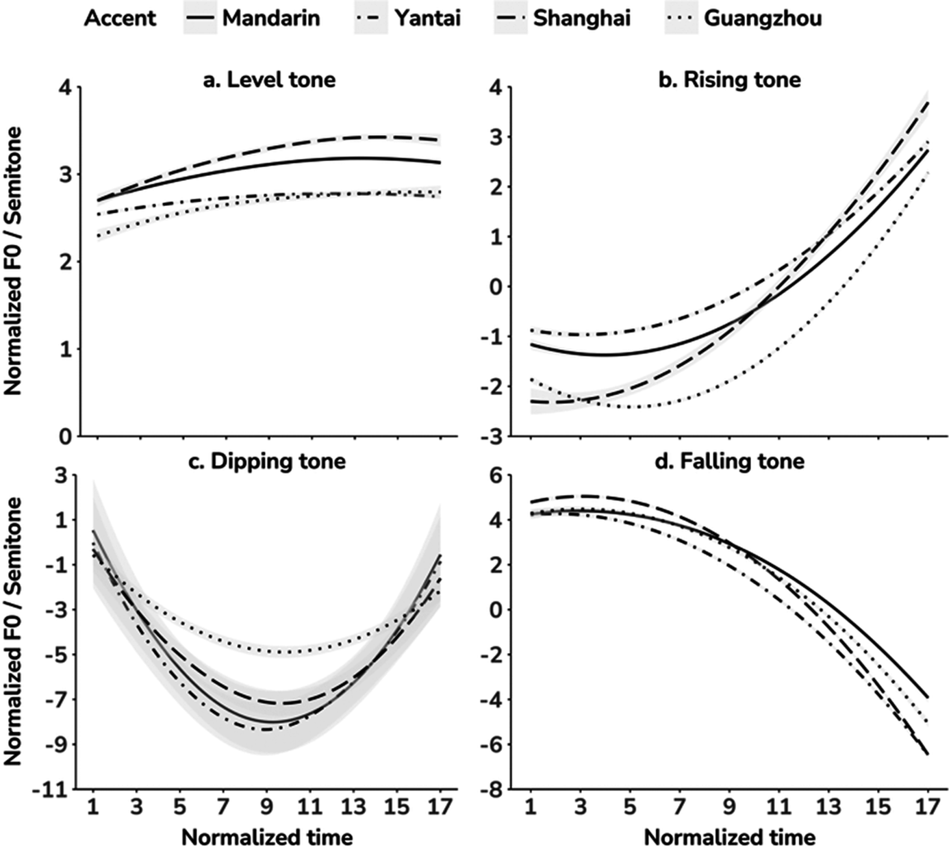
Regional talkers’ L2 pronunciation of Mandarin tones can deviate from native Mandarin norms due to influences of their L1s, which often have different tone systems from Beijing Mandarin and/or different phonetic realizations of shared tones. Yantai, Shanghai, and Guangzhou are different from each other, as well as from Mandarin (see Li et al., Reference Li, Best, Tyler, Burnham, Meng, Xu and Zheng2020b for more details about their differences in tone inventories), with differing tone inventories among them. Li et al. (Reference Li, Best, Tyler and Burnham2020a, Reference Li, Best, Tyler, Burnham, Meng, Xu and Zheng2020b) examined their productions of Mandarin tones in detail and found that while L2-Mandarin talkers from each region clearly distinguish the four tones, their productions of each tone deviate acoustically (phonetically) from L1-Mandarin, resulting in regionally accented Mandarin lexical tones. As shown in Figure 1, the F0 contours of the Mandarin level tone for L1-Mandarin and the three L2-Mandarin accents are all straight lines with high F0, but there are subtle rising or falling differences at some parts of the level tone’s F0 contours. Mandarin rising and falling tones show a trajectory of rising and falling, respectively, in all four accents, but the steepness of the slopes differs across accents. F0 contours of L2-Mandarin dipping tones in the Shanghai (long-dash line in Figure 1) and Guangzhou (dotted line) accents are shallower than those in L1-Mandarin (solid line) and Yantai L2-Mandarin (dot-dashed line). Moreover, the dipping curve in the Guangzhou accent is much shallower than that of the Shanghai accent, yielding an overall higher F0 height in Guangzhou. It is these F0 deviations that are expected to facilitate English learners’ tone-word learning and generalization to new talkers with a familiar and an unfamiliar accent in a high-variability training task that includes both accent and talker variability, as compared to those trained only with talker variability.
F0 variations of the Mandarin tones in L2-Mandarin accents in relation to the L1-Mandarin accent for the stimuli used in this study. Lines indicate the mean normalized F0 contours across four talkers of each accent in normalized time. The stimuli and this figure are adapted from Li et al. (Reference Li, Best, Tyler, Burnham, Meng, Xu and Zheng2020b).

Figure 1. Long description
A four-panel line graph displays normalized F 0 in semitones on the y-axis against normalized time on the x-axis. A legend at the top identifies four accents: Mandarin (solid line), Yantai (dashed line), Shanghai (dash-dotted line), and Guangzhou (dotted line).
* Panel a, Level tone: All accents show relatively flat or slightly arched contours between 2 and 4 semitones. Yantai is the highest, followed by Mandarin, while Shanghai and Guangzhou are lower and nearly overlapping.
* Panel b, Rising tone: Contours start between -3 and -1 semitones and rise sharply. Yantai reaches the highest peak near 4 semitones, while Guangzhou remains the lowest throughout the time scale.
* Panel c, Dipping tone: Contours show a U-shaped parabolic curve. They start near 0, drop to a trough between -5 and -9 semitones around time point 9, and rise again. Mandarin and Yantai have the deepest dips, while Guangzhou has the shallowest dip.
* Panel d, Falling tone: Contours start high between 4 and 5 semitones and show a concave downward decline. Mandarin maintains the highest F 0 during the fall, while Yantai and Shanghai drop more steeply to approximately -6 semitones by time point 17.
We extended previous research on L2 tone-word training with talker variability, by training native English speakers on Mandarin minimal-tone contrasts in a high-talker-variability tone-word learning task with either the Beijing accent alone (single accent) or with the Beijing, Yantai, and Guangzhou accents (multiple accents). We predicted:
-
1) Learners trained on words spoken in the Beijing, Yantai, and Guangzhou accents will achieve better tone-word identification than learners trained on words spoken in the Beijing accent only.
-
2) In the test of generalization to new talkers, learners trained on words spoken in Beijing, Yantai, and Guangzhou accents will identify tone-words more accurately than learners trained on the Beijing accent only, for both the familiar Beijing accent and especially for the unfamiliar Shanghai accent.
Materials and methods
Participants
Forty-eight L1-English speaking students were recruited online from Australian universities and randomly assigned to a single-accent (n = 24, M age = 24.5 years, SD = 5.8, 14 females) or multiple-accent (n = 24, M age = 25.5 years, SD = 5.1, 15 females) group. All had acquired English from birth, either in Australia (n = 46, 27 females) or in the United States (n = 2, 2 females). Some of them had learned other language(s) such as Spanish and/or French, but all were linguistically naïve to Mandarin or any other lexical tone languages. Because sensitivity to pitch height and contour (i.e., pitch aptitude) is necessary for the adequate perception and learning of lexical tones (Perrachione et al., Reference Perrachione, Lee, Ha and Wong2011; Wong & Perrachione, Reference Wong and Perrachione2007), all participants demonstrated high pitch aptitude, as evidenced by above-chance performance on a pre-training F0 height and contour discrimination test (see Supplementary Materials for details: https://doi.org/10.17605/OSF.IO/C6SBM). Given evidence that extensive musical training facilitates non-native tone perception and L2 tone-word learning (Laméris et al., Reference Laméris, Llompart and Post2024), only non-musicians were recruited (defined as having no more than three cumulative years of private lessons across any combination of instruments, Wong & Perrachione, Reference Wong and Perrachione2007). Their language and music backgrounds were self-reported through an online survey, which also confirmed that none of them had any speech or hearing disorders.
This study was approved by the Western Sydney University Human Research Ethics Committee (Ethics Reference ID: H13105). Participants signed informed consent prior to testing and received eGift smart cards or course credits for their participation.
Stimuli
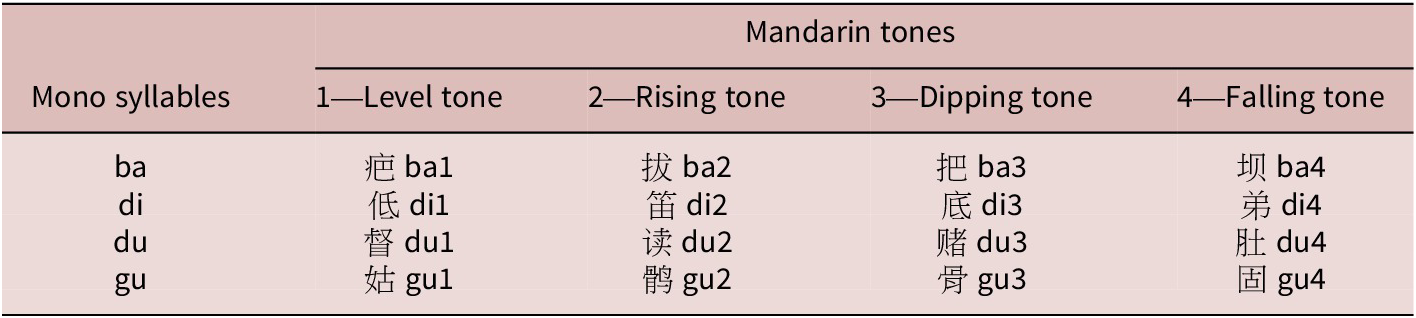
For the training and word identification tests, we selected 16 Mandarin words comprised of easily distinguished stop consonant-vowel (CV) syllables /ba/Footnote 1, /di/, /du/, and /gu/, combined with all four Mandarin tones (see Table 2). We included the dipping tone, which had been previously excluded in Perrachione et al. (Reference Perrachione, Lee, Ha and Wong2011) due to its confusion with the rising tone (Hao, Reference Hao2012). Our target lexicon instead reflected the full Mandarin tone system across multiple CV syllables, and thus was more challenging to learn than the 3-tone set used in Perrachione et al. (Reference Perrachione, Lee, Ha and Wong2011).
Monosyllabic Mandarin words used in tone-word training and identification tasks.

Table 2. Long description
The table is organized into five columns. The first column lists the base monosyllables, while the subsequent four columns represent Mandarin Tones 1 through 4.
* Row 1 Header: Monosyllables | 1 Level tone | 2 Rising tone | 3 Dipping tone | 4 Falling tone.
* Row 2: Syllable ba. Tone 1 is ba1. Tone 2 is ba2. Tone 3 is ba3. Tone 4 is ba4.
* Row 3: Syllable di. Tone 1 is di1. Tone 2 is di2. Tone 3 is di3. Tone 4 is di4.
* Row 4: Syllable du. Tone 1 is du1. Tone 2 is du2. Tone 3 is du3. Tone 4 is du4.
* Row 5: Syllable gu. Tone 1 is gu1. Tone 2 is gu2. Tone 3 is gu3. Tone 4 is gu4.
Each tonal entry includes the corresponding Chinese character followed by the syllable and tone number.
The single-accent training group (talker-only variability) were trained with multiple tokens of all target words by 12 L1 female talkers of Beijing Mandarin (M age = 21.83 years, SD = 1.99). The multiple-accent training group (talker and accent variability) were also trained with multiple tokens of all words by 12 female talkers (M age = 21.58 years, SD = 2.19), but the talkers were four L1 Mandarin talkers from Beijing (M age = 23.50 years, SD = 1.00) and four early-fluent L2-Mandarin talkers each from Yantai (M age = 21.25 years, SD = 1.50) and Guangzhou (M age = 19.75 years, SD = 1.26). Both training groups included recordings from 12 talkers, representing high-talker variability in both groups; they were differentiated only by the level of accent variability (one vs. four accents).
We recorded the target word materials from the native talkers under controlled conditions in a sound-attenuated booth at the Speech Acquisition and Intelligent Technology Lab, Beijing Language and Cultural University, China. Their productions were captured by a Shure SM57 dynamic microphone and recorded in Audacity (v. 2.3.0) on a Dell desktop computer at a 44.1-kHz sampling rate (32-bit resolution) via an M-audio M-track II external sound card. The Chinese characters displayed in Table 2 were presented individually per trial on an external monitor via E-Prime Professional 2.0 (Psychology Software Tools, Inc.) running on a Dell Latitude 7280 laptop. Each talker recorded 10 tokens of each word, once each per 10 recording blocks, yielding 160 trials per talker (16 words × 10 blocked repetitions), with the 16 words within each block presented in randomized order. Recordings were high-pass filtered at 70 Hz and manually segmented into individual utterances using Praat (Boersma & Weenink, Reference Boersma and Weenink2018). The resulting stimuli were subsequently used in an accent-similarity test, administered in E-Prime on a Dell OptiPlex 3030 AIO desktop computer and presented over AKG K272 headphones. Accent similarity was verified by four new Beijing L1-Mandarin listeners for the Beijing accent, and by four new Yantai and four new Guangzhou L2-Mandarin listeners for the Yantai and Guangzhou accents, respectively. Listeners rated how similar each Mandarin-word pronunciation was to that of their native region on a 7-point Likert scale (1 = not at all similar, 7 = highly similar). For each talker and training condition, the four tokens of each word receiving the highest similarity ratings were selected for use in the training study, resulting in a total of 768 stimuli (12 talkers × 16 pseudowords × 4 tokens).
For investigating the generalization of the trained words to new talkers of the familiar Beijing accent and the unfamiliar (untrained) Shanghai accent, multiple tokens of the 16 Mandarin words in Table 2 were recorded by two additional female talkers as described above, one a 13th L1 talker of Beijing Mandarin (19.00 years; familiar accent) and the other an early fluent L2-Mandarin talker from Shanghai (24.00 years; unfamiliar accent). Neither talker was presented to the participants during training before the generalization tests, i.e., both were new talkers. As before, four tokens per word by each of the new talkers were selected for the post-training generalization tests, yielding 64 tokens per talker (16 words × 4 tokens). As with the training stimuli, the selected tokens were verified by four new Beijing L1-Mandarin or four new Shanghai L2-Mandarin female talkers.
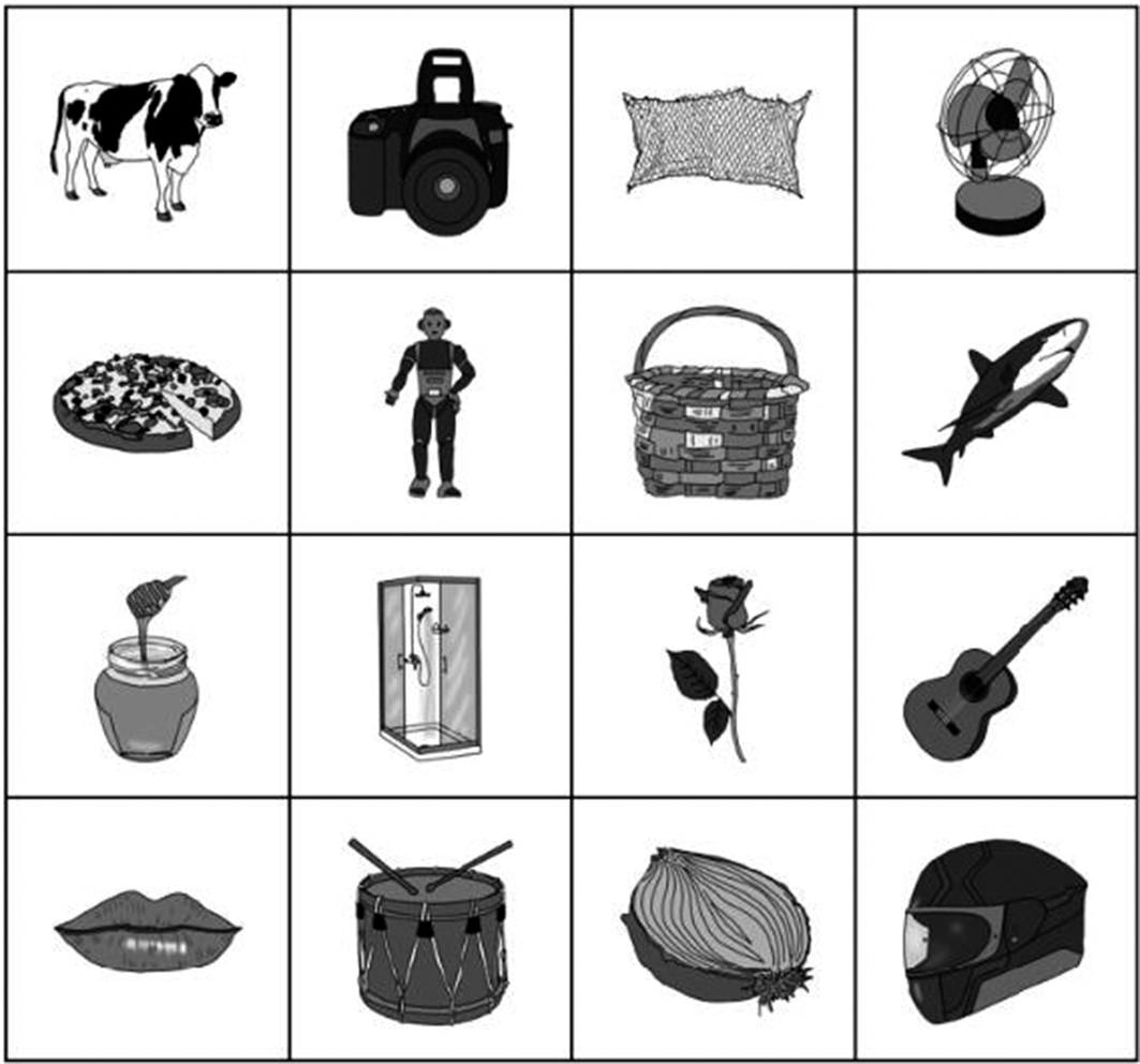
Since our task required easily recognizable objects, the assigned English meanings for the 16 words were arbitrary, resulting in Mandarin pseudowords. The meanings (see Figure 2), which referred to depictable concrete objects with moderate to high word frequency, were selected from van Heuven et al. (Reference van Heuven, Mandera, Keuleers and Brysbaert2014). They were depicted with gray-scaled drawings with high naming agreement and low visual complexity selected from the Multilingual Picture (MultiPic) database (Duñabeitia et al., Reference Duñabeitia, Crepaldi, Meyer, New, Pliatsikas, Smolka and Brysbaert2018). Word-meaning pairings were counterbalanced across participants (e.g., the cow corresponded to different Mandarin words such as 疤 /ba1/ and 拔 /ba2/ for different participants).
The 16 drawings for training.

Figure 2. Long description
The grid is organized into four rows and four columns.
Row 1 from left to right: a cow with black patches, a digital single-lens reflex camera, a rectangular mesh net, and an electric desk fan.
Row 2 from left to right: a pizza with one slice partially cut, a humanoid robot standing upright, a woven wicker basket with a handle, and a shark swimming toward the right.
Row 3 from left to right: a jar of honey with a wooden dipper, a glass-walled shower cubicle, a single rose with leaves on its stem, and an acoustic guitar.
Row 4 from left to right: a pair of human lips, a snare drum with two drumsticks resting on top, a cross-section of an onion showing its internal layers, and a motorcycle helmet with a visor.
Procedure
The participants completed six training sessions on the 16 pseudowords over six consecutive days with a sound-to-meaning paradigm adapted from Wong and Perrachione (Reference Wong and Perrachione2007). Each training session presented four talkers of the same accent (approximately 45 min), yielding three sessions for a total of 12 talkers. Set order was counterbalanced across participants, and those three sessions (Sessions 1–3: Block 1) were repeated a second time (Sessions 4–6: Block 2) for a total of six sessions to ensure sufficient training as recommended in Wong and Perrachione (Reference Wong and Perrachione2007). The 12 Beijing Mandarin talkers for the single-accent group were randomly assigned to the three sessions per block, and the four talkers each of the Beijing, Yantai, and Guangzhou accents in the multiple-accent group were blocked by session. There were 256 randomized trials (4 talkers × 4 syllables × 4 tones × 4 tokens) in each session with 16 words blocked by talker (n = 4) to optimize word learning (Perrachione et al., Reference Perrachione, Lee, Ha and Wong2011). For the same reason, talker blocks were further subdivided by syllable (i.e., by minimal-tone-contrast word set), yielding 16 randomized trials per word set (4 words × 4 tokens). Talker and syllable orders within talker were randomized across participants.
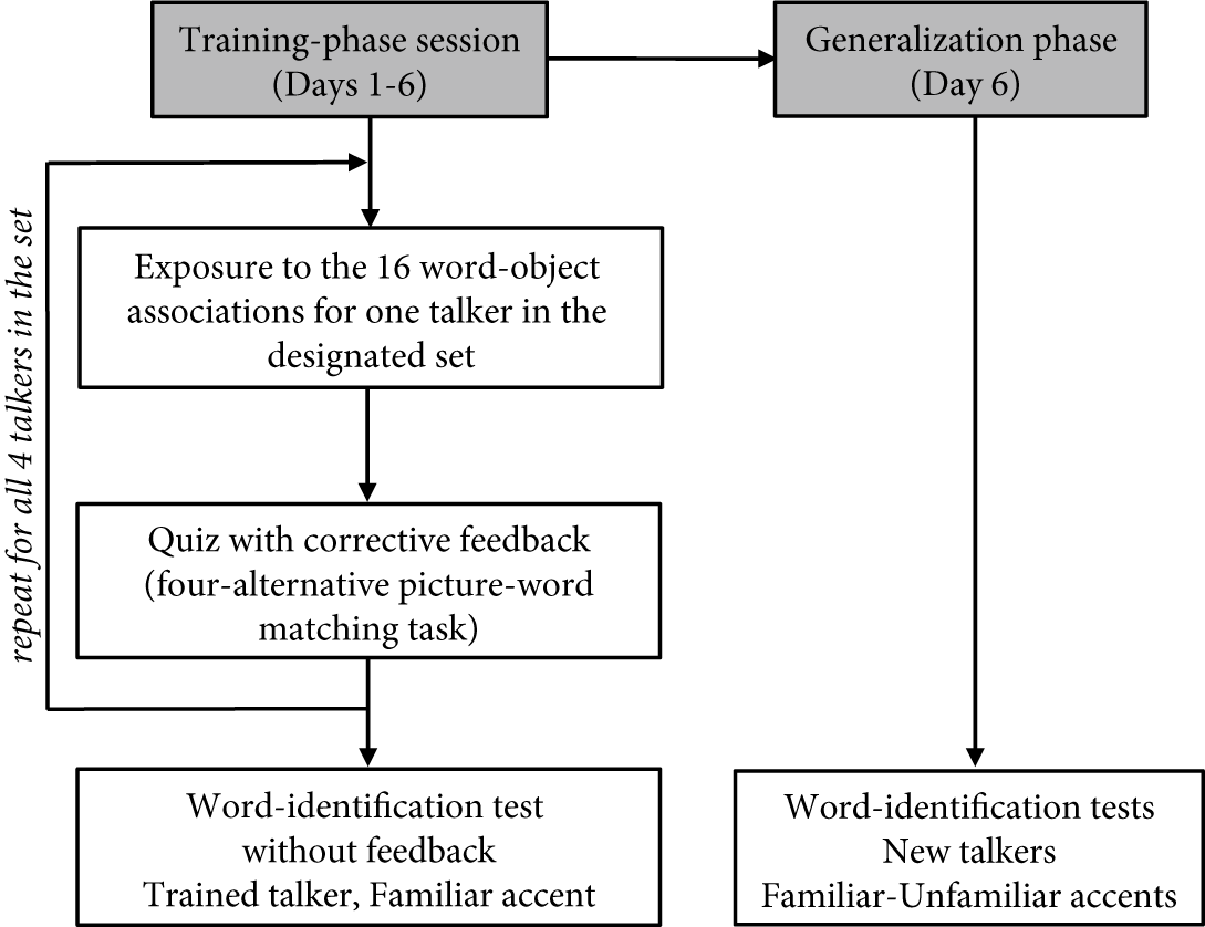
On each tone-word training trial, the target object image was displayed, starting 0.5 s earlier than the paired word began; the image remained on screen during the word presentation. Learners were instructed to remember as many word-meaning pairs as possible. After training on the four minimal-tone-contrast words of a syllable set by a given talker, they completed a corresponding 16-trial quiz. In each quiz trial, they heard one target word and had to choose the correct item in the display of four drawings. Correct answers were followed by a green tick on the screen and incorrect answers by a red cross mark. If the participant gave no response within 5.5 s, a reminder appeared asking them to respond more quickly. Following wrong or no answers, the correct drawing and audio word were presented to facilitate tone-word training (Laméris et al., Reference Laméris, Llompart and Post2024). Participants then were trained and quizzed on the 16 words produced by each of the other three talkers of the set, with the same cycle as shown in the second and third rectangles in the left panel of Figure 3.
Summary of the experimental protocol.

Figure 3. Long description
The flowchart is organized into two main columns representing different experimental phases.
1. Training-phase session (Days 1-6): Located at the top left in a gray box. An arrow points down to a white box labeled ‘Exposure to the 16 word-object associations for one talker in the designated set’.
2. Training Loop: An arrow points down to a second white box labeled ‘Quiz with corrective feedback (four-alternative picture-word matching task)'. A return arrow on the left side loops back to the exposure step, labeled ‘repeat for all 4 talkers in the set’.
3. Training Outcome: An arrow from the quiz box points down to a final white box at the bottom left labeled ‘Word-identification test without feedback: Trained talker, Familiar accent’.
4. Generalization phase (Day 6): A horizontal arrow from the top-left gray box points to a top-right gray box labeled ‘Generalization phase (Day 6)'.
5. Generalization Outcome: A long vertical arrow points from the generalization phase box down to a white box at the bottom right labeled ‘Word-identification tests: New talkers, Familiar-Unfamiliar accents’.
To track learning progress across the six sessions, learners completed tone-word identification tests at the end of each session with 64 randomized trials (16 words × 4 tokens) (Figure 3, bottom left). The four tokens per word were one each from the four talkers of a given session to maintain talker variation, and token per talker per word was counterbalanced across learners to include token variation. On a given trial, learners saw the 16 pictures, which were displayed on a 4 × 4 answer matrix (as shown in Figure 2) on the participant’s computer screen, where syllables and tones were blocked by row and column, respectively, and they heard a token depicting one of the 16 pictures. The item positions in the answer display were counterbalanced across participants but were constant across sessions for each participant.
After hearing the word, learners were instructed to identify the word by clicking on the correct picture. To ensure each tone-word was heard in full before an identification judgment was made, learners had to activate each trial by pressing and holding a mouse-click on a centered button on the screen until they heard the full stimulus. If they released it too soon, the trial ended automatically with a reminder to respond after hearing the word. Terminated trials (139 occurrences, or 0.7% of all trials across learners and sessions) were repeated in a random order at the end of each test. In contrast to the quizzes within training sessions, identification tests provided no feedback. To encourage careful thinking, there was no timeout, but learners responded within 5.5 s on average.
Immediately after the word-identification test of the final training session, learners completed generalization tests to new talkers of the familiar Beijing and the unfamiliar Shanghai accents, in that order, following the same word-identification procedure (Figure 3, bottom right). Only 38 trials (0.6%) were terminated by premature mouse click release. These two tests took about 7 min to complete.
Participants completed the training and testing online using their own laptop computer. The experimenter supervised the sessions via ZOOM to ensure data quality. The experiment was controlled using E-Prime Go (Psychology Software Tools, Inc.), which set the display resolution at 1920 × 1080. Stimuli were presented via the participant’s wired earphones or headphones, which they adjusted to comfortable loudness during a pre-test practice session.
Statistical analysis
Bayesian mixed-effects models were used to analyze the perceptual data, because they account for cross-participant and cross-item effects, and prove measures of evidence regarding the hypotheses under investigation. This is particularly valuable in our study, where graded evidence for learning effects across sessions is more informative than simply determining whether effects are statistically significant. All models were implemented using the brms package in R (v. 4.4.0) (R Core Team, 2024).
We used a Bernoulli logit link to predict correct versus incorrect identification based on the training group, the session, and their interaction for learning and generalization data. This approach is well-suited for analyzing categorical response data and allows for interpretable estimates of changes in accuracy over time. We also included predictors for trial number to account for fatigue effects, and how often a specific stimulus had been presented to account for token familiarity (Herff et al., Reference Herff, Olsen and Dean2018). All models included random intercepts for participant. Continuous variables were standardized to a mean of 0 and a standard deviation of 1. We used weakly informative priors in the form of t distributions with a mean of 0, a standard deviation of 1, and 3 degrees of freedom (Gelman et al., Reference Gelman, Jakulin, Pittau and Su2008). R-hat was used to assess convergence, and all R-hats were 1 throughout (Bürkner, Reference Bürkner2017). This approach has commonly been applied in auditory perception studies (Escudero et al., Reference Escudero, Smit and Angwin2023; Milne & Herff, Reference Milne and Herff2020) both within and outside the linguistics domain.
To understand the separate contributions of tones and syllables in the current design, we scored tone and syllable accuracy separately: a response was counted as correct for the syllable even if the tone was incorrect, and vice versa. We then applied the same modeling architecture as above to the separated tone accuracy and syllable accuracy data, but added a ToneOrSyllable factor that interacted with session and accent group. We used the package marginaleffects to identify posterior predictions of the model and performed hypothesis tests on them to assess the factors of interest and their interactions. For these hypothesis tests, we reported regression coefficients (β), their estimate error (EEβ), evidence ratios (ERs) for directional effects (Odds(β > or β < 0)), and the corresponding posterior probabilities (Post.Prob). Following Milne and Herff (Reference Milne and Herff2020), ERs greater than 19 were taken to indicate strong evidence for a directed hypothesis. This threshold reflects the relative support for the hypothesized effect over its alternative, with larger values indicating stronger evidence. Full posterior summaries are provided in the Supplementary Materials. For convenience, we denoted effects with “*” that can be considered “significant” at an α = .05 level.
Results
Mandarin minimal-tone-contrast word learning and identification
Overall word learning and identification
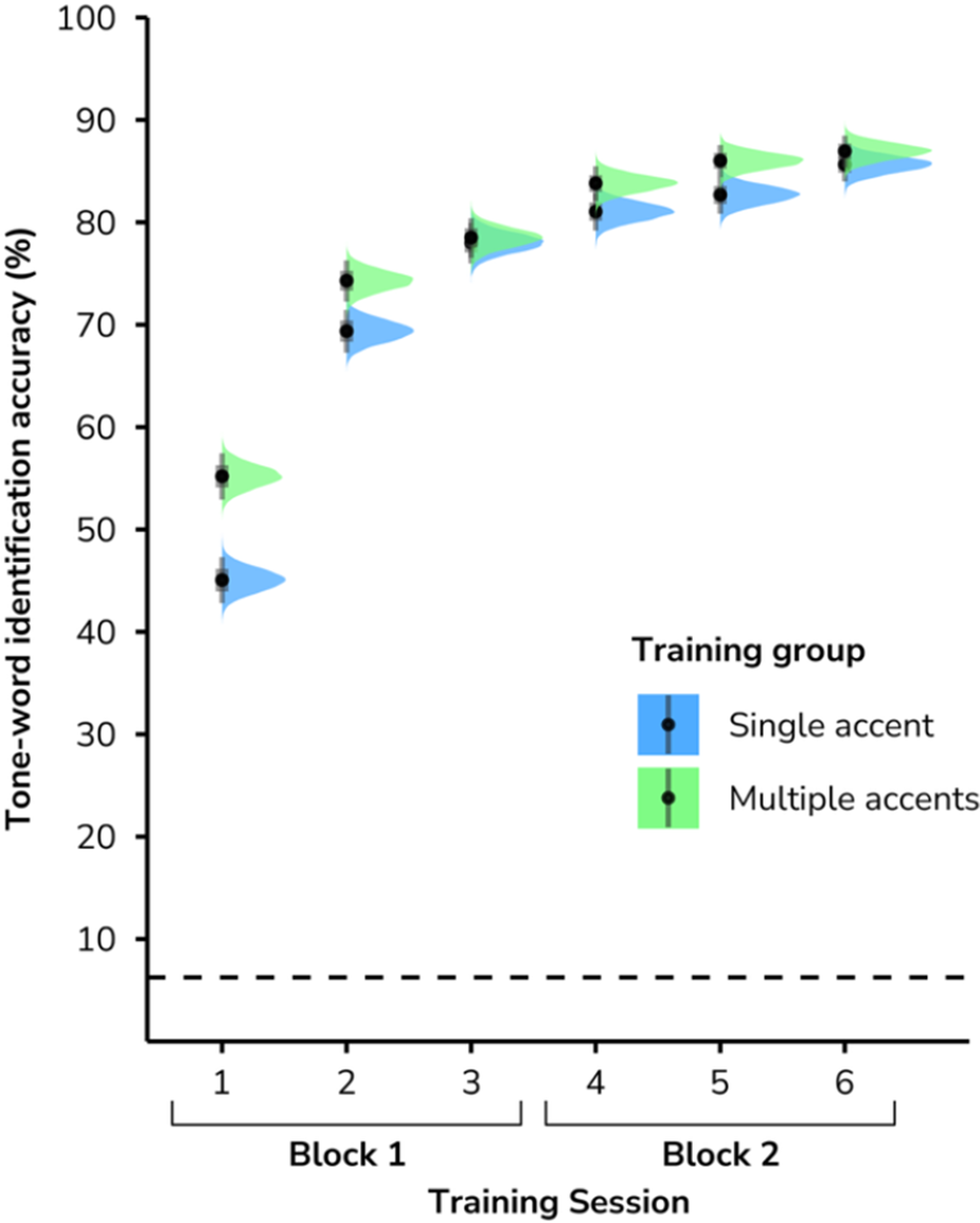
The Bayesian models of the identification test data from the six training sessions provided strong evidence that both the single- (β = 0.41, EEβ = 0.01, Odds(β > 0) = 9999*, Post.Prob = 1.00) and multiple-accent (β = 0.32, EEβ = 0.01, Odds(β > 0) > 9999*, Post.Prob = 1.00) groups improved from the first (M single-accent = 44.54%, SD = 22.50 vs. M multiple-accent = 55.33%, SD = 23.33) to the final (M single-accent = 85.75%, SD = 13.52 vs. M multiple-accent = 86.96%, SD = 9.36) training session (see Figure 4).
Posterior distributions of expected predictions for training effects on tone-word identification accuracy by single-accent versus multiple-accent groups. The dashed line indicates chance level.

Figure 4. Long description
The y-axis represents Tone-word identification accuracy % ranging from 0 to 100. The x-axis represents Training Session numbered 1 through 6, divided into Block 1 (sessions 1 to 3) and Block 2 (sessions 4 to 6). A horizontal dashed line at approximately 6% indicates the chance level.
A legend identifies two groups: Single accent (blue) and Multiple accents (green). Each data point includes a central dot for the mean, vertical error bars, and a horizontal half-violin plot (raincloud) showing the distribution.
Data trends:
* Session 1: Multiple accents group starts higher at approximately 55% compared to Single accent at approximately 45%.
* Session 2: Both groups improve, with Multiple accents at approximately 74% and Single accent at approximately 69%.
* Session 3: The groups converge at approximately 78%.
* Session 4: Multiple accents group reaches approximately 84% while Single accent is slightly lower at approximately 81%.
* Session 5: Multiple accents is at approximately 86% and Single accent is at approximately 83%.
* Session 6: Both groups reach their peak, with Multiple accents at approximately 87% and Single accent at approximately 86%.
Overall, both groups show a logarithmic growth curve, with the Multiple accents group maintaining a slight performance advantage in most sessions.
There was also strong evidence illustrating that both groups improved across sessions in Block 1 (Sessions 1–3, M single-accent = 33.62%, SD = 22.52 vs. M multiple-accent = 23.04%, SD = 18.88; Single-accent: β = 0.33, EEβ = 0.02, Odds(β > 0) > 9999*, Post.Prob = 1.00; Multiple-accent: β = 0.23, EEβ = 0.02, Odds(β > 0) > 9999*, Post.Prob = 1.00), and across sessions in Block 2 (Sessions 4–6, M single-accent = 4.67%, SD = 6.34 vs. M multiple-accent = 3.21%, SD = 15.62; Single-accent: β = 0.05, EEβ = 0.01, Odds(β > 0) > 9999*, Post.Prob = 1.00; Multiple-accent: β = 0.03, EEβ = 0.01, Odds(β > 0) = 203.08*, Post.Prob = 1.00). The Bayesian models also provided strong evidence that, except for Sessions 3 and 6 (the final sessions of Blocks 1 and 2), the multiple-accent group performed better than the single-accent group (all ERs > 19 for Sessions 1, 2, 4, and 5), indicating a consistent performance advantage for the multiple-accent group across training sessions. Both groups had reached asymptotic performance in each training block by the second session of that block, with small additional improvement in the final session of each block.
Performance split by tone and syllable
To examine whether tone and/or syllable learning contributed to group differences, the responses were rescored to give separate tone and syllable identification accuracies. These overall tone and syllable scores were then broken down by individual tones and syllables to assess the effects of accent variability on specific tone and syllable learning.
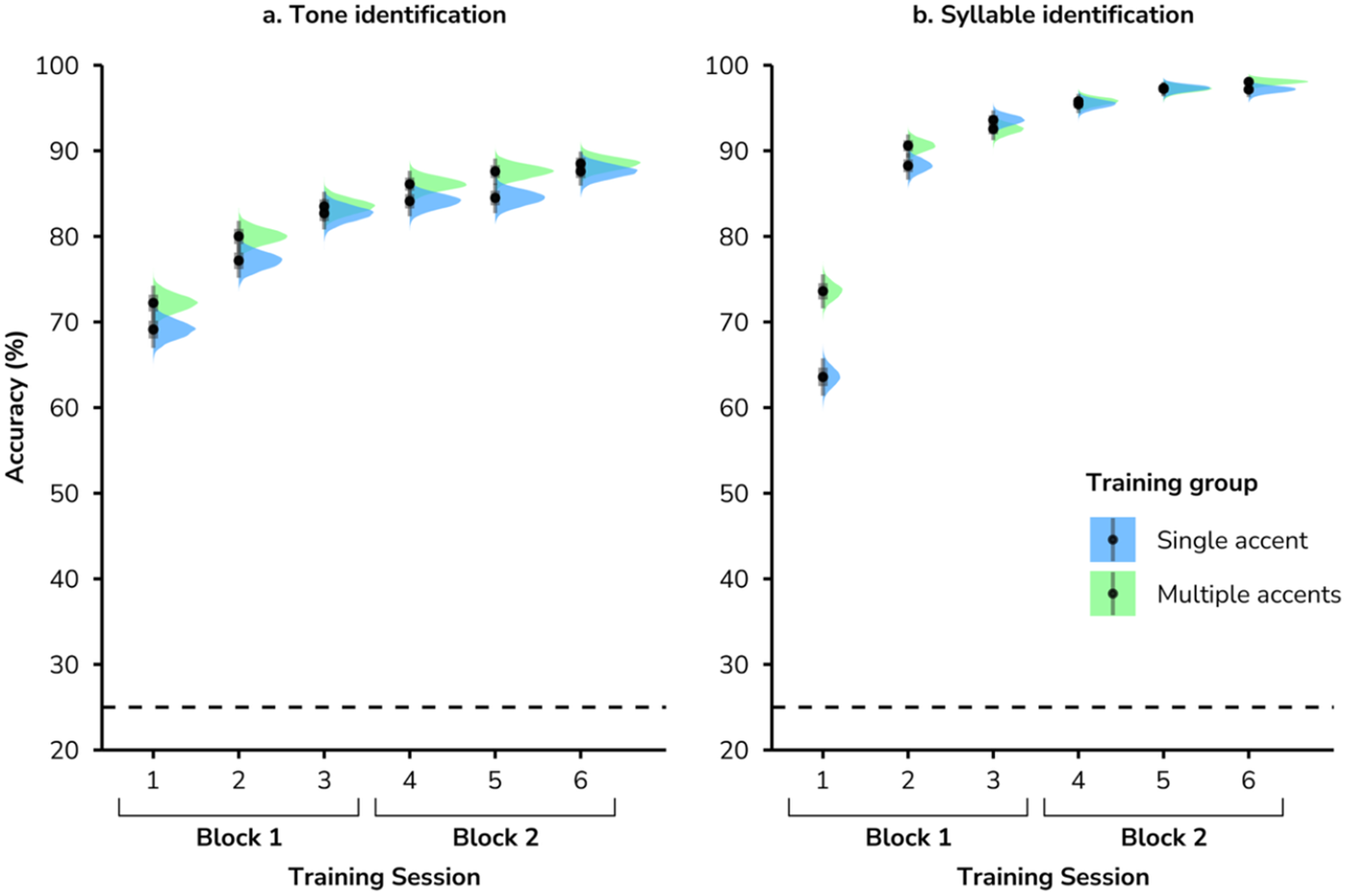
As shown in Figure 5, both groups improved tone identification gradually from the first session (M single-accent = 69.71%, SD = 15.07 vs. M multiple-accent = 71.96%, SD = 18.05) to the sixth session (M single-accent = 87.50%, SD = 11.96 vs. M multiple-accent = 88.46%, SD = 8.94) for approximately 17 percentage points (M single-accent = 17.79%, SD = 14.07; M multiple-accent = 16.50%, SD = 15.40), with greater improvement in Block 1 (M single-accent = 12.92%, SD = 13.22; M multiple-accent = 11.58%, SD = 12.87) than Block 2 (M single-accent = 3.50%, SD = 6.40; M multiple-accent = 2.33%, SD = 11.26). Again, we observed strong evidence for these improvements (all ERs > 19). We also observed strong evidence, again, that the multiple-accent group performed better than the single-accent group in all sessions except for the final session in each block (Sessions 3 and 6).
Posterior distributions for training effects on tone and syllable accuracy by single-accent versus multiple-accent groups. The dashed line indicates chance level.

Figure 5. Long description
The figure consists of two side-by-side panels, labeled a and b. Both panels share a Y-axis representing Accuracy percentage from 20 to 100 and an X-axis representing Training Session from 1 to 6. A dashed horizontal line at 25 percent indicates chance level. Sessions 1 through 3 are grouped as Block 1, and sessions 4 through 6 are grouped as Block 2.
Panel a, Tone identification: Accuracy for both groups starts between 65 and 75 percent in Session 1 and shows a steady logarithmic increase to nearly 90 percent by Session 6. The multiple-accent group (green) consistently maintains a slightly higher mean accuracy than the single-accent group (blue) across all sessions.
Panel b, Syllable identification: The multiple-accent group starts significantly higher (approximately 74 percent) than the single-accent group (approximately 64 percent) in Session 1. Both groups show rapid improvement, converging at approximately 95 to 98 percent accuracy by Session 6.
A legend in the bottom right of panel b identifies the blue violin plots with a black dot as Single accent and the green violin plots with a black dot as Multiple accents. Each data point includes a vertical error bar and a horizontal density distribution.
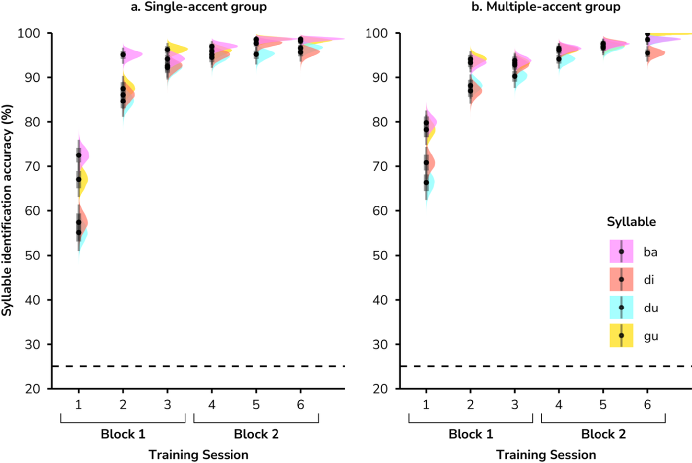
Similar to tone identification, we observed strong evidence that both groups improved syllable identification from Sessions 1 to 6 as well as within block improvements (all ERs > 19). There was also strong evidence that the multiple-accent group performed better initially, in Session 1 (M single-accent = 62.50%, SD = 23.04 vs. M multiple-accent = 73.88%, SD = 23.00; β = 0.10, EEβ = 0.01, Odds(β > 0) > 9999*, Post.Prob = 1.00). The syllable analysis broken down by individual syllables (see Figure 6) showed that the multiple-accent group outperformed the single-accent group in identifying all four syllables (all ERs > 19). Both groups achieved over 88% mean syllable accuracy by Session 2, i.e., their performance asymptoted well before the final session even though it continued to show small improvements from Session 2 to Session 6 (M single-accent = 97.17%, SD = 5.55 vs. M multiple-accent = 97.96%, SD = 2.61). Together, these findings suggest that improvements in tone-word learning across training sessions were driven primarily by gains in tone identification rather than in syllable learning.
Posterior distributions for training effects on syllable identification accuracy by syllable and accent group. The dashed line indicates chance level.

Figure 6. Long description
Two side-by-side panels labeled a. Single-accent group and b. Multiple-accent group.
Axes and Layout:
* The Y-axis represents Syllable identification accuracy percentage from 20 to 100.
* A horizontal dashed line at 25 percent indicates the chance level.
* The X-axis represents Training Session numbered 1 through 6.
* Sessions 1, 2, and 3 are grouped under Block 1.
* Sessions 4, 5, and 6 are grouped under Block 2.
Data Trends:
* In both panels, accuracy shows a steep logarithmic increase from Session 1 to Session 3, followed by an asymptotic plateau near 100 percent in Block 2.
* Each data point consists of a central black dot with a vertical error bar, flanked by a colored density distribution (half-violin plot).
* In Panel A, the syllable ba (pink) starts significantly higher in Session 1 (around 72 percent) compared to other syllables which cluster between 55 and 68 percent.
* In Panel B, all syllables are more tightly clustered in Session 1, ranging from approximately 65 to 80 percent.
Legend:
Located in the bottom right of Panel B, the Syllable legend identifies four categories:
* ba: pink
* di: coral
* du: cyan
* gu: yellow
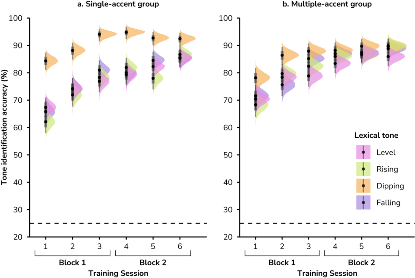
For identification accuracy of the four tones (see Figure 7), both groups showed improvements from the first to the sixth training session for each tone (all ERs > 19). While the single-accent group outperformed the multiple-accent group in identifying dipping tone after Session 1 (M single-accent = 84.38%, SD = 36.36 vs. M multiple-accent = 78.13%, SD = 41.39; β = 0.06, EEβ = 0.02, Odds(β > 0) = 231.56*, Post.Prob = 1.00), the multiple-accent group outperformed the single-accent group in identifying rising (M single-accent = 61.72%, SD = 48.67 vs. M multiple-accent = 68.23%, SD = 46.62; β = 0.06, EEβ = 0.03, Odds(β > 0) = 49.76*, Post.Prob = 0.98) and falling (M single-accent = 65.36%, SD = 47.64 vs. M multiple-accent = 71.61%, SD = 45.15; β = 0.06, EEβ = 0.03, Odds(β > 0) = 43.44*, Post.Prob = 0.98) tones. The multiple-accent group retained higher rising-tone identification accuracy than the single-accent group until Session 5 (M single-accent = 77.86%, SD = 41.57 vs. M multiple-accent = 86.72%, SD = 33.98; β = 0.09, EEβ = 0.03, Odds(β > 0) = 2499.00*, Post.Prob = 1.00). However, by Session 6, both groups reached equivalent performance on the four tones. Across the four tones, we observed strong evidence that both groups demonstrated the highest identification accuracy for the dipping tone after Session 1, and higher accuracy for the dipping tone than for the level tone at Session 6 (all ERs > 19). These results suggest that dipping tone is learned more easily than the other three tones when paired with lexical meanings.
Posterior distributions for training effects on tone identification by tone and accent group. The dashed line indicates chance level.

Figure 7. Long description
The figure consists of two side-by-side panels, labeled a. Single-accent group and b. Multiple-accent group. Both panels share a Y-axis titled Tone identification accuracy % ranging from 20 to 100, and an X-axis titled Training Session with six sessions divided into Block 1 (sessions 1 to 3) and Block 2 (sessions 4 to 6). A horizontal dashed line at 25% indicates the chance level.
Data is presented as posterior distributions (violin plots) with central points and error bars for four lexical tones: Level (pink), Rising (green), Dipping (orange), and Falling (purple).
* Panel a (Single-accent group): The Dipping tone (orange) starts highest at approximately 85% in session 1 and improves to nearly 95% by session 6. The other three tones (Level, Rising, Falling) start much lower, clustered between 60% and 70% in session 1, showing a steep linear increase through Block 1 and plateauing between 80% and 88% in Block 2.
* Panel b (Multiple-accent group): All four tones show a more compressed distribution compared to panel a. The Dipping tone (orange) remains the highest performing, starting near 78% and reaching 90%. The Level, Rising, and Falling tones start between 68% and 72% and converge toward 85% to 90% by session 6. The overall improvement slope is more gradual than in the single-accent group.
A legend in the bottom right of panel b identifies the colors for Level, Rising, Dipping, and Falling tones.
Generalization to new talkers of a familiar and an unfamiliar accent
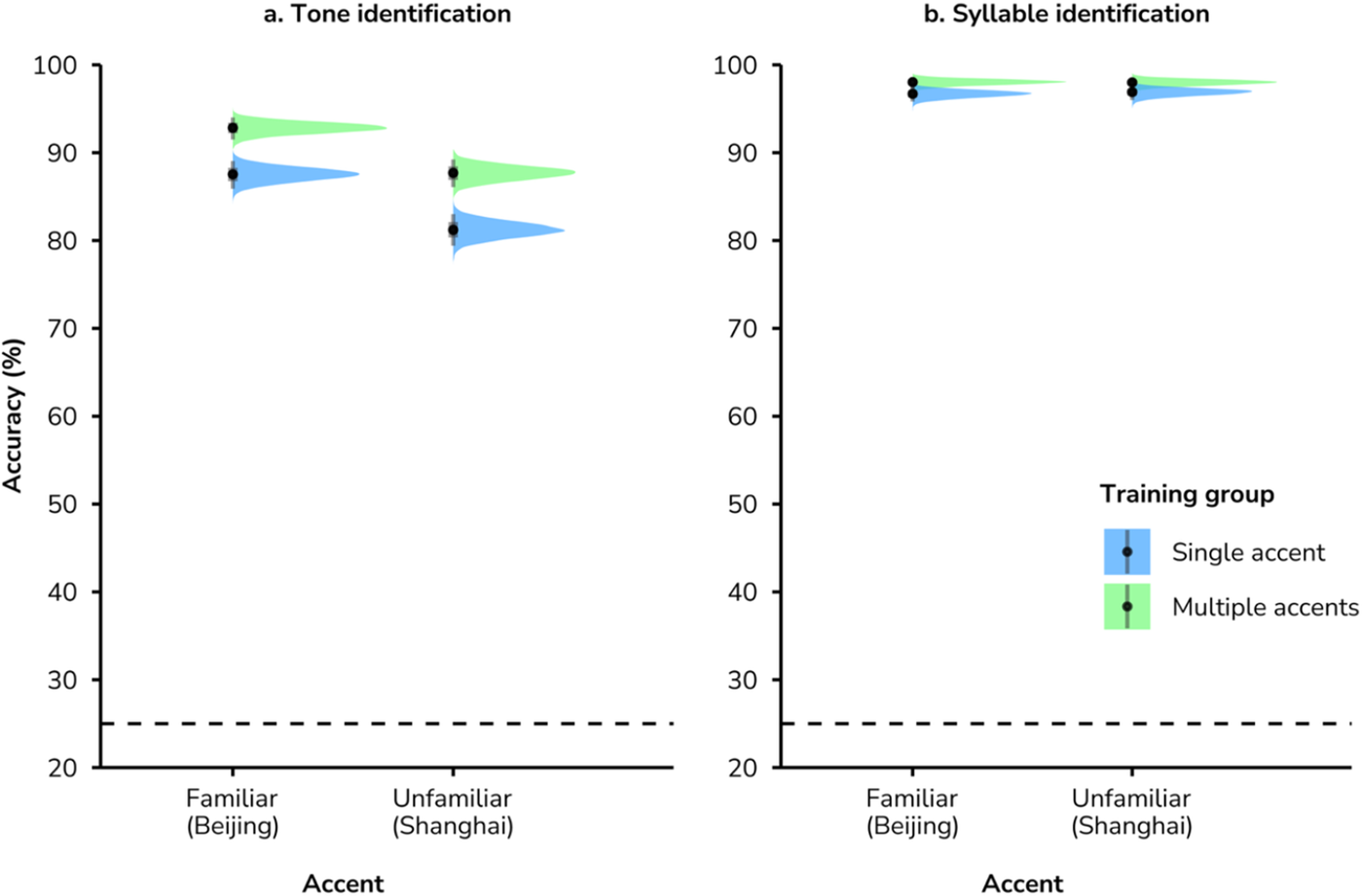
We focused here on the split accuracy for tones and for syllables (see Figure 8), as we were interested in generalization of phonological abstraction for lexical tones and syllables to new talkers from Beijing and Shanghai. As a reminder, both the single-accent group and the multiple-accent group had been trained on the Beijing accent, and neither group was trained on the Shanghai accent. The data analysis method was similar to that in Mandarin tone-word identification tests.
Posterior distributions for tone- and syllable-identification accuracy in generalization tests to new talkers with a familiar Beijing versus an unfamiliar Shanghai accent. The dashed line indicates chance level.

Figure 8. Long description
A two-panel violin plot. Both panels share a Y-axis labeled Accuracy % ranging from 20 to 100, with a dashed horizontal line at 25 indicating chance level. The X-axis for both panels lists Familiar Beijing and Unfamiliar Shanghai accents.
Panel a, Tone identification. For the Beijing accent, the Multiple accents group (green) shows a peak near 93% accuracy, while the Single accent group (blue) is lower at approximately 88%. For the Shanghai accent, both groups show a decrease in performance, with the Multiple accents group at roughly 88% and the Single accent group at 81%.
Panel b, Syllable identification. Performance is significantly higher and more stable across conditions. For both Beijing and Shanghai accents, both training groups cluster tightly between 95% and 98% accuracy, with the Multiple accents group (green) consistently slightly higher than the Single accent group (blue).
A legend in the bottom right of panel b identifies the blue violin with a black dot as Single accent and the green violin with a black dot as Multiple accents.
There was strong evidence that exposure to multiple accents during word training resulted in better tone generalization than single-accent training for both the new talker with the familiar Beijing accent (see Figure 8a; M single-accent = 87.46%, SD = 11.36 vs. M multiple-accent = 92.88%, SD = 5.80; β = 0.05, EEβ = 0.01, Odds(β > 0) > 9999*, Post.Prob = 1.00), and the new talker with the unfamiliar Shanghai accent (M single-accent = 81.08%, SD = 13.35 vs. M multiple-accent = 87.67%, SD = 9.43; β = 0.06, EEβ = 0.01, Odds(β > 0) > 9999*, Post.Prob = 1.00). There was also strong evidence that both groups showed slightly better generalization to the new talker with the familiar Beijing accent than to the new talker with the unfamiliar Shanghai accent (Single-accent: β = 0.06, EEβ = 0.01, Odds(β > 0) = 9999*, Post.Prob = 1.00; Multiple-accent: β = 0.05, EEβ = 0.01, Odds(β > 0) = 9999*, Post.Prob = 1.00).
For syllable processing, both groups achieved 95% accuracy (see Figure 8b) in generalizations to new talkers of the familiar Beijing accent (M single-accent = 96.54%, SD = 5.47 vs. M multiple-accent = 97.96%, SD = 3.62) and of the unfamiliar Shanghai accent (M single-accent = 96.83%, SD = 6.65 vs. M multiple-accent = 97.88%, SD = 2.91). Accordingly, we did not find significant evidence that participants performed better in generalization of syllables to the new talker of the familiar accent than to the new talker of the unfamiliar accent. Nevertheless, similar to tone identification, there was strong evidence that the multiple accent group performed better than the single accent group in the two generalization tests (Beijing: β = 0.01, EEβ = 0.01, Odds(β > 0) = 242.90*, Post.Prob = 1.00; Shanghai: β = 0.01, EEβ = 0.01, Odds(β > 0) = 52.48*, Post.Prob = 0.98).
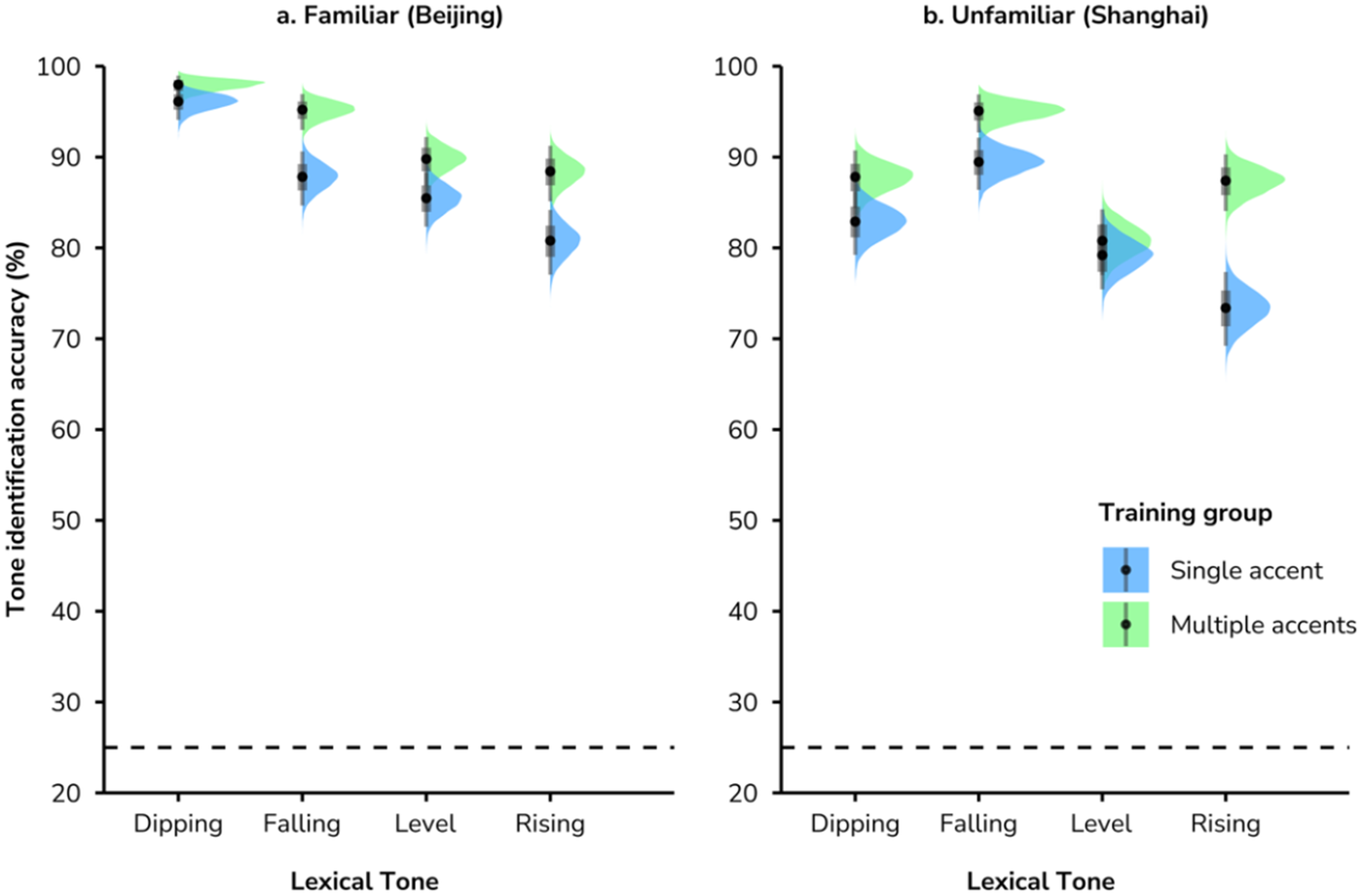
Figure 9 shows group differences broken down by specific tone. For generalization to the new talker with a familiar accent, the multiple-accent group outperformed the single-accent group in identifying all four tones, i.e., level (M single-accent = 85.16%, SD = 35.60 vs. M multiple-accent = 89.84%, SD = 30.25), rising (M single-accent = 80.73%, SD = 39.49 vs. M multiple-accent = 88.28%, SD = 32.21), dipping (M single-accent = 96.61%, SD = 18.11 vs. M multiple-accent = 97.92%, SD = 14.30), and falling (M single-accent = 87.50%, SD = 33.12 vs. M multiple-accent = 95.31%, SD = 21.16) tones. For generalization to the new talker with an unfamiliar accent, the multiple accent group showed higher identification accuracy for the rising (M single-accent = 73.18%, SD = 44.36 vs. M multiple-accent = 87.50%, SD = 33.12), dipping (M single = 82.55%, SD = 38.00 vs. M multiple = 87.76%, SD = 32.82), and falling (M single-accent = 89.58%, SD = 30.59 vs. M multiple-accent = 95.05%, SD = 21.71) tones. All effects were strong (all ERs > 19). We also found that both groups demonstrated higher identification accuracy for the level and falling tones when generalizing to the new talker with the familiar accent than to the one with an unfamiliar accent (all ERs > 19). In addition, the single-accent group showed better identification of the rising tone for generalization to the familiar-accent talker than to the unfamiliar-accent talker (β = 0.07, EEβ = 0.03, Odds(β > 0) = 255.41*, Post.Prob = 1.00). Across the four tones, both groups achieved the highest identification accuracy for the dipping tone when generalizing to the new talker with a familiar accent, whereas the highest accuracy for generalization to the new talker with an unfamiliar accent was observed for the falling tone. All effects showed strong evidence (all ERs > 19).
Posterior distributions for tone-identification accuracy in generalization tests involving new talkers with familiar Beijing versus unfamiliar Shanghai accents, split by tone. The dashed line indicates chance level.

Figure 9. Long description
A two-panel raincloud plot. Both panels share a y-axis labeled Tone identification accuracy % ranging from 20 to 100 and an x-axis labeled Lexical Tone with four categories: Dipping, Falling, Level, and Rising. A dashed horizontal line at 25% indicates the chance level.
Panel a, titled Familiar Beijing:
* For all four tones, the Multiple accents group (green) shows higher accuracy than the Single accent group (blue).
* Accuracy is highest for Dipping (near 95-98%) and lowest for Rising (near 80-88%).
* Data distributions are narrow and concentrated at the top of the scale.
Panel b, titled Unfamiliar Shanghai:
* The Multiple accents group (green) consistently outperforms the Single accent group (blue) across all tones.
* The performance gap is most pronounced in the Falling and Rising tones.
* Overall accuracy is lower than in the Beijing panel, with the Single accent group dropping to approximately 73% for the Rising tone.
A legend in the bottom right of panel b identifies the blue markers and distributions as Single accent and the green markers and distributions as Multiple accents. Each data point includes a central dot for the mean, a thick vertical bar for the interquartile range, and a shaded density plot to the right.
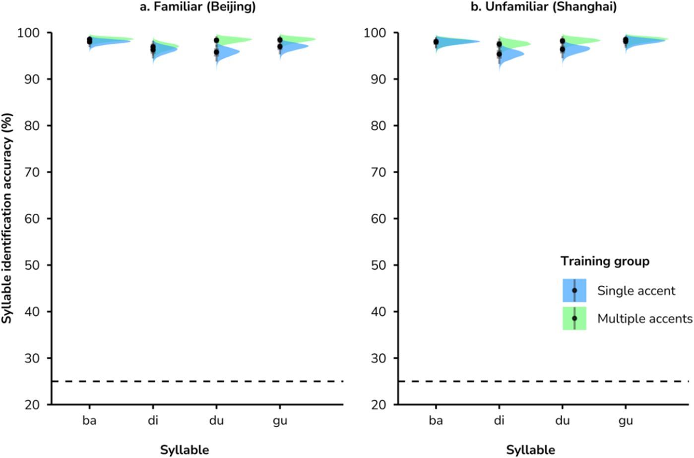
For syllable contributions to group differences (see Figure 10), there was strong evidence that in generalization to the new talker of the familiar Beijing accent the multiple-accent group performed better than the single-accent group in identifying words with the syllables /du/ (M single-accent = 95.31%, SD = 21.16 vs. M multiple-accent = 98.44%, SD = 12.42; β = 0.03, EEβ = 0.01, Odds(β > 0) = 195.08*, Post.Prob = 0.99) and /gu/ (M single-accent = 96.61%, SD = 18.11 vs. M multiple-accent = 98.44%, SD = 12.42; β = 0.01, EEβ = 0.01, Odds(β > 0) = 20.46*, Post.Prob = 0.95). In generalization to the new talker of the unfamiliar Shanghai accent, the multiple-accent group outperformed the single-accent group in identifying words with the syllables /du/ (M single-accent = 96.35%, SD = 18.77 vs. M multiple-accent = 98.18%, SD = 13.40; β = 0.02, EEβ = 0.01, Odds(β > 0) = 26.55*, Post.Prob = 0.96) and /di/ (M single-accent = 95.05%, SD = 21.71 vs. M multiple-accent = 97.66%, SD = 15.15; β = 0.02, EEβ = 0.01, Odds(β > 0) = 26.62*, Post.Prob = 0.96).
Posterior distributions for syllable-identification accuracy in generalization tests involving new talkers with familiar Beijing versus unfamiliar Shanghai accents, split by syllable. The dashed line indicates chance level.

Figure 10. Long description
A two-panel graph with Panel A on the left titled Familiar Beijing and Panel B on the right titled Unfamiliar Shanghai.
Both panels share identical axes. The y-axis represents Syllable identification accuracy percentage ranging from 20 to 100 with a dashed horizontal line at 25 indicating chance level. The x-axis is labeled Syllable with four categories: ba, di, du, and gu.
A legend in Panel B identifies two training groups: Single accent represented by blue violin plots with black dots and Multiple accents represented by green violin plots with black dots.
In Panel A (Beijing):
* For ba, di, du, and gu, all data points for both Single and Multiple accent groups are clustered near the top of the scale between 95 and 100 percent accuracy.
* The blue and green distributions are highly overlapping and narrow, indicating high precision and ceiling-level performance.
In Panel B (Shanghai):
* The data follows a similar pattern to Panel A with all syllables showing accuracy above 90 percent.
* For the syllable di, the Single accent group (blue) shows a slightly wider distribution and a marginally lower mean dot compared to the Multiple accents group (green), though both remain very high.
* For ba, du, and gu, the distributions for both training groups are nearly identical and concentrated at the top of the y-axis.
Discussion
The present study investigated the effects of accent variability on monolingual English perceivers’ acquisition of Mandarin minimal-tone-contrast words. Participants completed six sessions of tone-word training, and their learning trajectories were tracked using word-identification tests administered after each session. They subsequently completed two generalization tests to new talkers with a familiar Beijing and an unfamiliar Shanghai accent.
Both the single-accent and multiple-accent groups reached around 85% accuracy by the final training session having asymptoted by the third session, despite completing fewer training sessions (six in our study) than the nine sessions used in Chandrasekaran et al. (Reference Chandrasekaran, Sampath and Wong2010) and Wong and Perrachione (Reference Wong and Perrachione2007). These results indicate that our modified training program was both effective and efficient for tone-word training, further supported by the high levels of dipping-based word identification observed in both groups. Notably, the multiple-accent group outperformed the single-accent group during the first two sessions of each training block. This early advantage was primarily driven by tone identification, as both groups reached 88+% accuracy in syllable identification by the second session. Because the multiple-accent group had already been exposed to accent variability during the initial two sessions of Block 1, their superior tone identification in those sessions (as well as the first two sessions of Block 2) suggests that exposure to multiple accents facilitated the extraction of more stable abstract representations of lexical tones. In other words, accent variability appears to promote the emergence of phonological constancy at an early stage of tone-word learning. However, this advantage diminished by the third session, as both groups reached nearly 80% accuracy regardless of accent condition. This convergence suggests that talker variability alone, experienced by both groups, was highly effective and that additional accent variability provided an early but relatively modest enhancement. Our prediction regarding the effect of accent variability on tone-word learning was therefore modestly supported. The high identification accuracy achieved by the final session of Block 2 in training further suggested that both groups had established abstract phonological representations of the lexical tones, which were subsequently evaluated in the two generalization tests.
Both groups maintained ceiling-level syllable identification in the two generalization tests, suggesting that the tone-naïve English learners had established robust abstract phonological representations of the four trained Mandarin syllables. Thus, overall word identification accuracy primarily depended on tone identification, consistent with previous studies on Mandarin tone-word learning by English learners (Hao, Reference Hao2024; Pelzl et al., Reference Pelzl, Lau, Guo and DeKeyser2021). As predicted, the multiple-accent group outperformed the single-accent group in generalizing to the new talkers with both a familiar Beijing and an unfamiliar Shanghai accent. This advantage indicates that exposure to accent variability during tone-word training facilitated a more robust emergence of phonological constancy across talkers and accents. This pattern was further supported by tone-specific analyses: the multiple-accent group showed superior identification of all four tones in the familiar-accent condition and of three tones (all except the level tone) in the unfamiliar-accent condition. Interestingly, across the two generalization tests, both groups showed an overall advantage in the familiar-accent condition over the unfamiliar-accent condition, suggesting that phonological constancy had emerged but remained sensitive to accent familiarity. This finding is consistent with accent adaptation studies (Bradlow & Bent, Reference Bradlow and Bent2008; Clarke & Garrett, Reference Clarke and Garrett2004), as well as with meta-analytic evidence on the generalization effects of high-variability phonetic training (Uchihara et al., Reference Uchihara, Karas and Thomson2025). Although learners were able to generalize to new talkers, performance was facilitated when the accent matched previously experienced acoustic distributions. This pattern indicates that tone representations were abstract enough to support cross-talker generalization, yet not fully accent-invariant, particularly in the single-accent group, reflecting a gradual emergence of phonological constancy.
The present study advanced the perceptual attunement account (Best, Reference Best, Romero and Riera2015) by demonstrating that structured indexical variability plays a critical role in L2 tone-word learning. Because F0 movement in lexical tones is intrinsically tied to talker and accent variation (Li et al., Reference Li, Best, Tyler and Burnham2020a, Reference Li, Best, Tyler, Burnham, Meng, Xu and Zheng2020b), successful tone acquisition requires learners to abstract invariant cues from notably variable input. Our findings showed that English learners achieved such abstraction across both talker and accent differences, extending the scope of perceptual attunement beyond consonant and vowel perception (Best et al., Reference Best, Tyler, Gooding, Orlando and Quann2009) to lexical tone processing. Accent variability conferred greater generalization benefits than talker variability alone, underscoring the privileged role of higher-level indexical variation (Tyler & Best, Reference Tyler and Bestin preparation; see also Foulkes & Hay, Reference Foulkes, Hay, O’Grady and MacWhinney2015) in promoting phonological constancy. The observed generalization patterns provided strong support for hybrid models of word recognition (Cutler & Weber, Reference Cutler, Weber, Trouvain and Barry2007; Goldinger, Reference Goldinger, Trouvain and Barry2007), indicating that L2 tone representations simultaneously retain indexical detail and undergo progressive abstraction. These results indicate that phonological constancy in L2 tone learning is not the product of mere exposure but emerges through handling structured variability in the input as a fundamentally graded and dynamic process.
Beyond the establishment of new tone categories, the extent to which these representations generalize may depend on the acoustic relationship between training and test accents. Previous work demonstrates that cross-talker generalization is modulated by acoustic similarity among talker voices, with greater similarity facilitating transfer (Xie et al., Reference Xie, Liu and Jaeger2021; Xie & Myers, Reference Xie and Myers2017). Extending this logic to the accent level, if the Shanghai accent occupies an intermediate acoustic position relative to the training accents (see Figure 1), generalization performance may reflect graded similarity rather than categorical transfer. From this perspective, the observed multiple-accent advantage may represent a conservative estimate of variability effects: larger acoustic distances between training and test accents could further amplify the role of structured variability in promoting phonological constancy. Future research that systematically manipulates accent distance (see Bent et al., Reference Bent, Henry, Holt and Lind-Combs2024) in lexical tones would clarify how similarity at different levels of the indexical hierarchy (Tyler & Best, Reference Tyler and Bestin preparation; see also Foulkes & Hay, Reference Foulkes, Hay, O’Grady and MacWhinney2015) constrains variability-driven abstraction. Importantly, taken together, the generalization findings indicate the emergence of phonological constancy in L2 tone-word learning, suggesting that learners established abstract tone representations at the sub-lexical level. While the present study demonstrated the emergence of such abstraction across talkers and accents, future research could more directly assess this change by examining tone identification and discrimination of untrained tone-words following tone-word training (Chandrasekaran et al., Reference Chandrasekaran, Sampath and Wong2010; see also Li et al., Reference Li, Best, Tyler, Burnham and Billington2022, Reference Li, Tyler, Burnham and Best2023a). Meanwhile, long-term stability of phonological abstraction for tones in lexical contexts remains an open question. While a recent study has provided meta-analytic evidence on the long-term retention effects of high-variability phonetic training (Uchihara et al., Reference Uchihara, Karas and Thomson2025), delayed post-tests would offer a complementary approach to examining the durability of accent-variability-driven abstraction over time. Investigating how phonological constancy stabilizes or evolves beyond the initial learning phase would further refine theoretical models of L2 lexical tone acquisition.
The findings in this study contribute to our understanding of variability-based learning in L2 tone perception, and several important questions remain for future research. The present study used isolated monosyllabic minimal-tone-contrast words to ensure experimental control. Mandarin tones in natural speech interact with segmental context, prosodic structure, coarticulation, and intonation, and processes such as tone sandhi (see Duanmu, Reference Duanmu2007, for a review), all of which may alter their acoustic realization and perceptual salience. It remains to be determined whether the benefits of high-accent variability extend to sentence- or discourse-level contexts. In addition, because this study focused exclusively on monolingual English listeners, whose L1 lacks lexical tone, it remains unclear whether the facilitative effects of accent variability are specific to non-tone language learners or whether they generalize across learners with different L1 backgrounds. Cross-linguistic comparisons among tone-language learners (e.g., Cantonese, Thai), pitch-accent-language learners (e.g., Swedish, Japanese), and non-tone-language learners (Laméris et al., Reference Laméris, Llompart and Post2024) would clarify whether prior experience with lexical pitch distinctions modulates sensitivity to accent variability in lexical tones and the benefits derived from high-accent-variability input.
In sum, the present findings demonstrated that structured accent variability systematically enhances the robustness of L2 tone representations at the sub-lexical level. Rather than yielding fully invariant categories, accent variability promoted progressively abstract yet indexically informed representations. These results provided direct evidence that perceptual attunement in adult L2 tone learning is variability-driven, gradient, and fundamentally shaped by the structure of the input.
Data availability statement
The experiment in this article earned Open Data and Pre-Registered badges for transparent practices. The data are available at https://doi.org/10.17605/OSF.IO/C6SBM.
Acknowledgments
The authors would like to gratefully acknowledge insightful comments from three anonymous reviewers, as well as Handling Editor Kazuya Saito and Editor Luke Plonsky, on earlier versions of the manuscript. This study was supported by a joint PhD scholarship from Western Sydney University (WSU) and the China Scholarship Council (CSC), as well as by Research Training Funds from the MARCS Institute for Brain, Behaviour and Development at WSU. It was also partly funded by two Australian Linguistic Society Research Grants awarded to the first author. Co-author Herff’s work on this report was supported by an Australian Research Council (ARC) Discovery Early Career Research Award (DECRA, DE220100961) and a Sydney Horizon Fellowship (University of Sydney). The authors would like to thank CareerHub at Australian Catholic University, Australian National University, The University of Melbourne, The University of Western Australia, and Western Sydney University for assisting with online recruitment of participants during the Covid-19 pandemic. The authors would also like to thank Johnson Chen, Dr. Chris Wang, and Dr. Gabriele Cecchetti for their technical support at the MARCS Institute for Brain, Behaviour and Development, as well as Professor Jinsong Zhang at the Speech Acquisition and Intelligent Technology (SAIT) Lab, Beijing Language and Culture University, China, for granting us access to the lab’s professional recording booth. Above all, we are grateful to the participants for their time and involvement. Parts of these findings were presented at the 20th International Congress of the Phonetic Science (ICPhS), Prague, Czech Republic, in August 2023 (Li et al., Reference Li, Tyler, Burnham, Best, Skarnitzl and Volín2023b).
Competing interests
The authors declare none.


 Open access

