
1. Introduction
Turbulent heat transfer is encountered in numerous industrial applications, and in most cases the turbulent heat exchange takes place in non-equilibrium flows. It is the case, for instance, for the surface air–oil heat exchangers implemented in modern aircraft engine by-pass ducts, where an essentially temperature-homogeneous flow makes contact with a heated surface, and is therefore abruptly subjected to a temperature gradient.
It was interest in the behaviour of the atmospheric boundary layer that first drew attention to turbulent heat transfer in non-equilibrium flows, both theoretically and experimentally (see Antonia, Danh & Prabhu Reference Antonia, Danh and Prabhu1977). The case where non-equilibrium is induced by a step change in surface temperature is the simplest example of non-equilibrium turbulent heat transfer, and numerous experimental works can be found in the literature. Johnson & Whippany (Reference Johnson and Whippany1957) studied the development of a thermal boundary layer on a smooth flat plate, and presented mean temperature and velocity profiles while focusing on fluctuating profiles in a later work (Johnson Reference Johnson1959). Blom (Reference Blom1970) carried out a similar study, comparing mean temperature profiles to the theoretical predictions of Spalding (Reference Spalding1961), and presenting the evolution of the turbulent Prandtl number. Similar experimental works can be found in Fulachier (Reference Fulachier1972), Hoffmann & Perry (Reference Hoffmann and Perry1979), Ng et al. (Reference Ng, Talbot, Cheng and Robben1983), Taylor et al. (Reference Taylor, Love, Coleman and Hosni1990) and, more recently, Biles et al. (Reference Biles, Ebadi, Allard and White2019), while Antonia et al. (Reference Antonia, Danh and Prabhu1977) and Teitel & Antonia (Reference Teitel and Antonia1993) studied the case of a step change in wall heat flux in a flat plate and turbulent channel flow configuration, respectively.
In spite of its Reynolds number limitation, direct numerical simulation (DNS) is undoubtedly the most accurate tool available for the investigation of turbulent heat transfer, since all the turbulent scales are solved. The first DNS addressing turbulent heat transfer is that of Kim & Moin (Reference Kim and Moin1989), where the transport of three passive scalars at different molecular Prandtl numbers is considered in a fully developed channel flow at a friction Reynolds number of  ${Re}_{\tau } = 180$. Several works followed, aiming at understanding the influence on the flow statistics of the Reynolds number and molecular Prandtl number (e.g. Papavassiliou & Hanratty Reference Papavassiliou and Hanratty1997; Kawamura, Abe & Matsuo Reference Kawamura, Abe and Matsuo1999; Abe, Kawamura & Matsuo Reference Abe, Kawamura and Matsuo2001), as well as of the isothermal or isoflux boundary conditions (e.g. Kasagi, Tomita & Kuroda Reference Kasagi, Tomita and Kuroda1992; Kawamura, Abe & Shingai Reference Kawamura, Abe and Shingai2000). Other authors focused on the coupling between turbulence and temperature gradient, an analysis which is possible only if temperature is handled as an active scalar. Most of these DNS were performed in supersonic channel flows (see Coleman, Kim & Moser Reference Coleman, Kim and Moser1995; Huang, Coleman & Bradshaw Reference Huang, Coleman and Bradshaw1995; Morinishi, Tamano & Nakabayashi Reference Morinishi, Tamano and Nakabayashi2004; Tamano & Morinishi Reference Tamano and Morinishi2006) while only a few focused on low speed flows with high temperature gradients (see Nicoud Reference Nicoud1999; Toutant & Bataille Reference Toutant and Bataille2013).
All the numerical works mentioned so far represent cases of equilibrium flows, and are undoubtedly the reference for understanding turbulent heat transfer in all its aspects (flow statistics, turbulent Prandtl number, wall scaling and much more). Nevertheless, questions arise concerning the validity of these findings in non-equilibrium configurations. Once more, DNS can be a powerful tool for the analysis of such flows, yet the literature is extremely less abundant on the matter. Seki & Kawamura (Reference Seki and Kawamura2005) performed the DNS of a fully developed channel flow with temperature as a passive scalar, where the wall temperature is constant everywhere but in a small fraction of the bottom wall, where it evolves along the streamwise direction attaining a peak. The step change of wall temperature significantly perturbs the mean and fluctuating temperature, as well as turbulent Prandtl number. Hattori, Houra & Nagano (Reference Hattori, Houra and Nagano2007), Hattori, Yamada & Houra (Reference Hattori, Yamada and Houra2012) and Hattori et al. (Reference Hattori, Yamada, Tanaka, Houra and Nagano2013) performed several DNS of non-equilibrium thermal boundary layers in the flat plate configuration. Hattori et al. (Reference Hattori, Houra and Nagano2007) analysed the effects of buoyancy on mean and fluctuating properties, as well as on the turbulent budgets for a turbulent boundary layer at equilibrium facing a step change in wall temperature. In Hattori et al. (Reference Hattori, Yamada and Houra2012), non-equilibrium is induced through the sudden vanishing of wall heat flux and, in one of the two cases presented, with the addition of a forward facing step. Similar analyses are carried out in Hattori et al. (Reference Hattori, Yamada, Tanaka, Houra and Nagano2013), yet temperature, in this case, is not handled as a passive scalar. Large-eddy simulation (LES) is certainly another valid tool for studying non-equilibrium turbulent heat transfer yet, despite the large turbulent scales being solved, a certain degree of modelling is needed for the smaller scales. Sanchez et al. (Reference Sanchez, Aulery, Toutant and Françoise2014) and Bellec, Toutant & Olalde (Reference Bellec, Toutant and Olalde2017) performed the LES of a temperature-homogeneous fully developed channel flow making contact with anisothermal walls for  ${Re}_{\tau } = 180$ and
 ${Re}_{\tau } = 395$, respectively. They showed the evolution of the mean and fluctuating temperature profiles, as well as the impact on the mean and fluctuating velocity components.
The objective of this paper is to deepen the knowledge of turbulent non-equilibrium heat transfer, which, as the literature review shows, has been investigated in a limited number of studies, especially in the case of flows with temperature-dependent properties. The intention is not only to describe and characterise a non-equilibrium flow, but also its gradual evolution towards a new equilibrium state.
To achieve the scope of the study, we perform the DNS of a channel flow, where a turbulent, fully developed, temperature-homogeneous flow at  ${Re}_{\tau } = 395$ makes contact with an isothermal wall. The step change in surface temperature leads to the development of a thermal layer, and, since temperature is an active scalar, the velocity boundary layer is also modified. The length of the isothermal wall allows the boundary layer to reach a new equilibrium state, characterised by a fully developed thermal boundary layer. The simulation is performed under one single flow regime, in terms of Reynolds number, Mach number and heat flux parameter. Nevertheless, the case is representative of a larger class of non-equilibrium flows where the thermal boundary layer responds to a sudden perturbation. Therefore, beyond the case-specific conditions, the study primarily aims at identifying the physical phenomena that are expected to be encountered in comparable non-equilibrium flows, while providing the theoretical means to understand them. In particular, we will see that the sudden perturbation is associated with (i) a local effect near the hot-wall leading edge specific to the change in wall temperature, and (ii) a more general subsequent longitudinal and transverse development of the boundary layer towards a new equilibrium.
The work is organised as follows. In § 2 the problem is described in detail; the governing equations are presented as well as details about the study configuration are given. In § 3 the numerical set-up and the proposed configuration are validated with respect to reference results found in the literature for equilibrium flows. In § 4 the results are presented. In § 4.1 the behaviour of the flow is analysed in what appears to be the most perturbed region, i.e. the leading edge of the isothermal wall. In § 4.2 an equilibrium region which characterises the development of the thermal boundary layer is identified and quantitatively defined. In § 4.3 the findings of § 4.2 are contrasted to the evolution of several turbulent quantities. This is followed by the conclusions in § 5.
2. Problem description
In this section details about governing equations and the numerical scheme (§ 2.1) as well as geometry, mesh and boundary conditions (§ 2.2) are given.
2.1. Governing equations and numerical scheme
The full compressible Navier–Stokes equations are solved in the fluid without any turbulence model. The set of equations are
 $$\begin{gather} \frac{\partial \rho}{\partial t} + \frac{\partial \rho u_i}{\partial x_i} = 0 , \end{gather}$$
 $$\begin{gather}\frac{\partial \rho u_i}{\partial t} + \frac{\partial \rho u_i u_j}{\partial x_j} ={-} \frac{\partial p}{\partial x_i} + \frac{\partial \boldsymbol{\tau}_{ij}}{\partial x_j} , \end{gather}$$
 \begin{gather} \frac{\partial \rho h}{\partial t} + \frac{\partial \rho u_j h}{\partial x_j} = \frac{\mathrm{D} p}{\mathrm{D} t} - \frac{\partial q^{cd}_j}{\partial x_j} + \boldsymbol{\tau}_{ij} \frac{\partial u_i}{\partial x_j} + S_{ener}, \end{gather}
where  $\rho$,
 $u_i$,
 $p$,
 $h$ are respectively the mass density, velocity components, static pressure and enthalpy per mass unit of the fluid; the fluid is considered to be an ideal gas with temperature-tabulated thermodynamic coefficients and mass-specific gas constant
 $r = 288.18$ J (kg.K)
 $^{-1}$ (assuming a mixture of
 $79\,\% \ \mathrm {N}_2$ and
 $21\,\% \ \mathrm {O}_2$) and state equation
 $p = \rho r T$, where
 $T$ is the static temperature; gravity is neglected and not included in momentum equation (2.2); the fluid is Newtonian and its dynamic viscosity
 $\mu$ is computed through the Sutherland law and is therefore temperature dependent; the conductive heat flux
 $q^{cd}_i$ follows the classic Fourier's law and the fluid thermal conductivity
 $\lambda$ is computed via the Prandtl number
 $Pr = 0.71$; finally,
 $S_{ener}$ is a source term added to the energy equation (2.3), the role of which will be clarified in § 2.2.
The set of equations is solved by the parallel code AVBP (Schonfeld & Rudgyard Reference Schonfeld and Rudgyard1999; Moureau et al. Reference Moureau, Lartigue, Sommerer, Angelberger, Colin and Poinsot2005) using a time-explicit finite-element two-step Taylor–Galerkin scheme (Colin & Rudgyard Reference Colin and Rudgyard2000) which provides third-order accuracy in space and time.
2.2. Geometry, mesh and boundary conditions
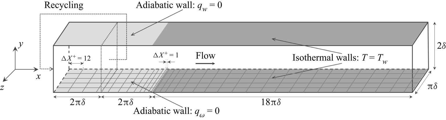
The geometry of the configuration studied is shown in figure 1. The computational domain is a channel flow of size  $22{\rm \pi} \delta \times 2\delta \times {\rm \pi}\delta$ (where
 $\delta = 0.002$ m) which is made of two parts in the streamwise direction.
Computational domain of the present study.

The upstream part has size  $4{\rm \pi} \delta \times 2\delta \times {\rm \pi}\delta$, the upper and lower walls (with respect to the
 $Y$ direction) are adiabatic, and a no-slip boundary condition is prescribed, while periodic boundary conditions are applied in the spanwise direction
 $Z$. Differently from what happens in biperiodic channel flows, in this case the flow is driven by a streamwise pressure gradient compensating the head losses generated along the whole domain shown in figure 1. In the
 $Z$ direction the mesh is uniform; in the wall-normal direction the mesh size, expressed in wall units, varies from
 $\Delta Y^+ = 0.75$ at the upper and lower walls to
 $\Delta Y^+ = 7$ at the centre of the channel; along the streamwise direction, the mesh size decreases with a constant ratio
 $1.05$ from
 $\Delta X^+ = 12$ at the inlet to
 $\Delta X^+ = 1$ at the interface with the downstream part of the channel flow (see figure 1). The role of this part of the domain is to generate a temperature-homogeneous boundary layer at equilibrium, with the regime conditions specified in table 1. In order to do so at a moderate cost, a recycling strategy is used: the three velocity components and the temperature imposed at the domain inlet via the Navier–Stokes characteristic boundary condition (NSCBC) formalism (Moureau et al. Reference Moureau, Lartigue, Sommerer, Angelberger, Colin and Poinsot2005; Poinsot & Veynante Reference Poinsot and Veynante2005) are extracted from a recycling plane situated downstream at a distance of
 $2{\rm \pi} \delta$. The energy source term
 $S_{ener}$ added to (2.3), is zero in this portion of the channel flow.
Size, mesh, spatial resolution and regime conditions of upstream (adiabatic) sub-domain:  $n_i$ is the number of grid points and
 $\Delta X_i^+$ the spatial resolution in wall units;
 ${Re}_{\tau }$ is the friction Reynolds number,
 $M$ the average Mach number and
 $T_b$ the bulk temperature.

The downstream part of the domain has size  $[18{\rm \pi} \delta, 2\delta, {\rm \pi}\delta ]$, the upper and lower walls are isothermal, both at temperature
 $T_w = 400$ K, and a no-slip boundary condition is prescribed, while, analogously to the upstream part, the domain is periodic in the spanwise direction. At the outlet, pressure is imposed via the NSCBC formalism. The mesh has the same point distribution of the upstream sub-domain along the
 $Y$ and
 $Z$ directions, while the mesh size increases with a constant ratio
 $1.05$ from
 $\Delta X^+ = 1$ at the adiabatic-isothermal interface until
 $\Delta X^+ = 12$ further downstream, where wall units are still referred to the adiabatic conditions of the upstream sub-domain, which are the most restrictive in terms of spatial resolution. This refinement along the streamwise direction serves to well capture the very first development region of the thermal boundary layer at the leading edge of the isothermal wall, where streamwise gradients can be important. The role of the downstream part is to allow the thermal boundary layer to be fully developed and to attain a new equilibrium state before the exit. The fully developed regime is characterised by a scaled mean temperature profile which is homogeneous in the streamwise direction. The role of the source term
 $S_{ener}$ added to the energy equation (2.3) is that of guaranteeing that a temperature gradient is preserved between the wall and the centre of the channel, allowing for a better appreciation of the fully developed regime. The mean temperature profile therefore results from the balance between the prescribed source term and the wall heat fluxes of the established flow
 $\overline {q_{w}}^{eq}$:
 \begin{equation} \overline{q_{w}}^{eq} \approx{-}S_{ener} \delta . \end{equation}
The source term  $S_{ener}$ takes a constant value specifically designed to obtain at equilibrium a bulk temperature of
 $T_b^{eq} = 304.5$ K, i.e. the same of the upstream part of the domain (see table 1), which yields a temperature of
 $T_c^{eq} \approx 290$ K at the centre of the channel. Thanks to (2.4), the value at equilibrium of the heat flux parameter
 $B_q$ and of the Nusselt number
 $Nu$ can be deduced,
 \begin{equation} B_{q}^{eq} ={-}\frac{\overline{q_{w}}^{eq}}{\rho_w c_{p_{w}} u_{\tau} T_w}, \quad Nu^{eq} ={-}2\delta \frac{\overline{q_{w}}^{eq}}{\lambda_w ( T_w - T_c )} , \end{equation}
where  $u_\tau = \sqrt {\tau _w/\rho _w}$, with
 $\tau _w$ the wall shear stress, is the friction velocity,
 $c_p$ is the constant-pressure specific heat and the subscript
 $(\cdot )_w$ denotes a fluid quantity taken at the wall.
Table 2 summarises the size and the mesh resolution, while table 3 details the regime conditions of the downstream part of the domain.
Size, mesh and spatial resolution of downstream (isothermal) sub-domain.

Regime conditions of downstream (isothermal) sub-domain. Here  $T_w / \bar {T}_{in}$ is the temperature ratio between the wall and the inlet.

3. Equilibrium states and validation
This study is characterised by two distinct equilibrium states, between which the flow evolves along the streamwise direction. The former is an adiabatic, fully developed turbulent flow in the upstream part of the domain; the latter is a fully developed turbulent thermal boundary layer at the outlet.
The objective of this section is twofold: first, to validate the numerical set-up introduced in § 2.1 with respect to reference results of the literature; second, to verify that the configuration described in § 2.2 allows us to meet the scope of the study, i.e. to observe the evolution of the boundary layer between the aforementioned equilibrium states.
In the following,  $(\bar {\cdot })$ and
 $(\tilde {\cdot })$ denote Reynolds and Favre averages, while
 $(\cdot )'$ and
 $(\cdot )''$ denote their respective fluctuating parts. Spatially, quantities are only averaged along the
 $Z$ axis, which is the only homogeneous direction for this configuration. Given the streamwise evolution of the boundary layer, unless specified, scaling of quantities (dimensionless numbers included) has to be intended locally with respect to the
 $X$ coordinate. The origin of the axes is placed at the interface between the adiabatic and isothermal walls, so that the non-dimensionalised
 $X$ coordinate
 $x/\delta$ is defined in the range
 $[-4{\rm \pi}, 18{\rm \pi} ]$ between the inlet and the outlet. The subscripts
 $(\cdot )_w$ and
 $(\cdot )_c$ indicate that the given property is evaluated at the wall and at the centre of the channel, respectively. The superscript
 $(\cdot )^+$ denotes classic wall scaling, that is,
 $$\begin{gather} y^+{=} \frac{\rho_w y u_{\tau}}{\mu_w} \quad \mathrm{and} \quad u_i^+{=} \frac{u_i}{u_\tau}\quad \mathrm{with}\quad u_\tau = \sqrt{\frac{\tau_w}{\rho_w}} , \end{gather}$$
 $$\begin{gather}T^+{=} \frac{| T - T_w |}{T_\tau} \quad \mathrm{with}\quad T_\tau = \frac{| q_w |}{\rho_w c_{p_{w}} u_{\tau}} . \end{gather}$$
The superscript  $(\cdot )^*$, instead, denotes semi-local scaling (see Huang et al. Reference Huang, Coleman and Bradshaw1995; Patel et al. Reference Patel, Peeters, Boersma and Pecnik2015), which uses local values (with respect to the wall-normal direction
 $Y$) of
 $\rho$,
 $\mu$ and
 $c_p$, instead of their values at the wall to account for variable properties
In the following sections, the behaviour of the flow is analysed at two streamwise locations: at  $x/\delta \approx 0$ in § 3.1, where an adiabatic, fully developed turbulent flow is expected; at
 $x/\delta \approx 18{\rm \pi}$ in § 3.2, where the development of the thermal boundary layer should be concluded.
3.1. Upstream equilibrium state
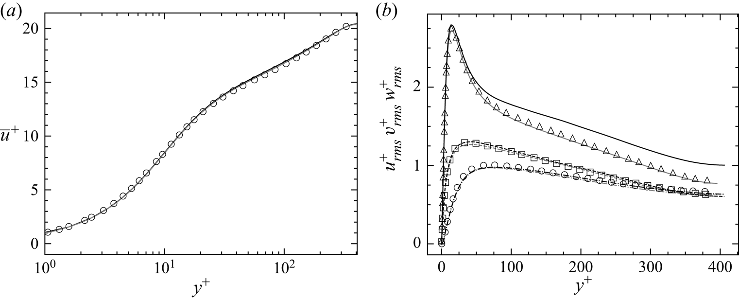
Figure 2 shows the mean streamwise velocity and the three root-mean-square (r.m.s.) velocity profiles at  $x/\delta = -0.1{\rm \pi}$, i.e. slightly downstream of the leading edge of the isothermal wall. Results at
 $x/\delta \approx 0$, represented by the black solid lines, are compared with two reference data. The first reference data, represented by the grey lines, have been obtained by simulating a classic biperiodic channel flow of size
 $[ 2{\rm \pi} \delta, 2\delta, {\rm \pi}\delta ]$ with the regime conditions of table 1; the second reference data, represented by the symbols, are taken from Kawamura et al. (Reference Kawamura, Abe and Shingai2000).
Upstream equilibrium state. Mean profile of streamwise velocity (a): ____ present results with  $2{\rm \pi} \delta$-long biperiodic channel flow (grey) and at
 $x/\delta \approx 0$ (black);
 $\bigcirc$ results from Kawamura et al. (Reference Kawamura, Abe and Matsuo1999). Profiles of r.m.s. streamwise, wall-normal and spanwise velocities, respectively (b): ____, –
 $\cdot$ –
 $\cdot$ – and - - - - present results (colours as above);
 $\triangle$,
 $\bigcirc$ and
 $\square$ results from Kawamura et al. (Reference Kawamura, Abe and Matsuo1999).

The collapsing between the small channel flow results and Kawamura et al. (Reference Kawamura, Abe and Shingai2000) is required to validate the numerical set-up of § 2.1; as can be seen, good agreement is obtained for both the mean streamwise velocity and the r.m.s. velocities.
The accord between the small channel flow and the present results at  $x/\delta \approx 0$, instead, is required to validate the study configuration described in § 2.2; excellent agreement is obtained on the mean streamwise velocity, which shows that the flow reaching the downstream part of the domain is a fully developed turbulent temperature-homogeneous boundary layer as desired; on the other hand, even though good agreement is obtained for the wall-normal and spanwise r.m.s. velocities, a disparity of around
 $10\,\%$ is observed for the streamwise component in the log layer; a possible explanation for this behaviour is given in the following section and, in more detail, in supplementary materials A, available at https://doi.org/10.1017/jfm.2021.1104.
3.2. Downstream equilibrium state
At  $x/\delta \approx 18{\rm \pi}$, the flow is expected to have evolved towards a new equilibrium state, characterised by a fully developed thermal boundary layer.
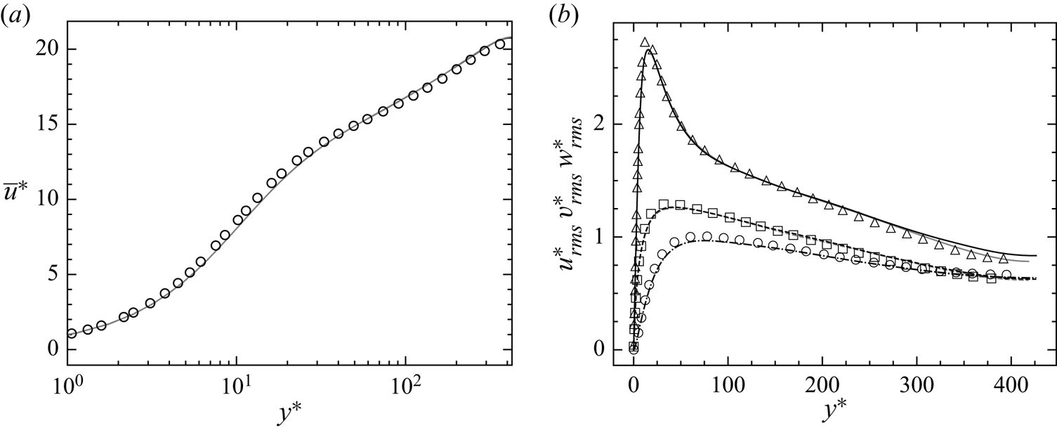
Figure 3 shows the mean streamwise and r.m.s.velocities at  $x/\delta = 287/16 {\rm \pi}$ compared with both the results of Kawamura et al. (Reference Kawamura, Abe and Matsuo1999) and, similarly to what is done in § 3.1, to the results obtained with a classic biperiodic channel flow at the regime conditions of table 3. Note that, in this case, semi-local scaling is used. As can be seen, good agreement is obtained for all the profiles, and even the streamwise r.m.s. velocity is considerably closer to the reference results. The disparity illustrated in figure 2(b) can thus be attributed to some local perturbation of the upstream flow, most probably induced by the recycling method described in § 2.2, the effects of which disappear further downstream.
Downstream equilibrium state. Profiles of mean streamwise (a) and r.m.s. streamwise, wall-normal and spanwise velocities (b) at  $x/\delta \approx 18{\rm \pi}$. See figure 2 for a reference to colours and symbols.

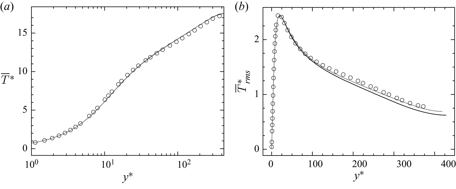
The profiles of the mean and r.m.s. temperature are instead shown in figure 4. Good agreement is obtained among all the curves for the mean temperature, while a slight discrepancy is observed on the r.m.s. profile. Therefore, if on the one hand the average thermal boundary layer seems to be fully developed at the outlet, on the other hand a longer isothermal wall would have been necessary to observe the same level of convergence for the temperature fluctuations.
Downstream equilibrium state. Profiles of mean (a) and r.m.s. (b) temperature: ____ present results with  $2{\rm \pi} \delta$-long biperiodic channel flow (grey) and at
 $x/\delta \approx 18{\rm \pi}$;
 $\bigcirc$ results from Kawamura et al. (Reference Kawamura, Abe and Matsuo1999).

Both figures 3 and 4 also illustrate how, thanks to semi-local scaling, fluid property variations in the wall-normal direction are properly taken into account, with all velocity and temperature profiles collapsing to those obtained by Kawamura et al. (Reference Kawamura, Abe and Matsuo1999) with a passive scalar. Fluid mean property variations, at least at equilibrium, seem thus to be the only remarkable impact of the heated wall on the flow, as suggested by Morkovin (Reference Morkovin1962) and seen in several studies involving compressible flows (e.g. Huang & Coleman Reference Huang and Coleman1994; Huang et al. Reference Huang, Coleman and Bradshaw1995; Nicoud Reference Nicoud1999).
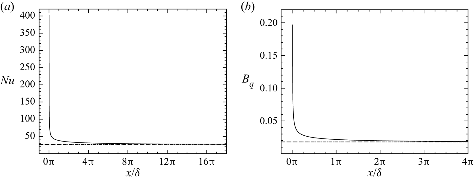
However, the effects of the temperature gradient on the flow can be much more important in other portions of the channel, namely in proximity of the leading edge of the isothermal wall. This can be seen in figure 5, which plots the evolution of the Nusselt number and of the heat flux parameter along the channel; both are very important near the leading edge, and the behaviour of the flow needs to be investigated in that region. The later convergence of  $Nu$ and
 $B_q$ towards the values of table 3, instead, provides further confirmation of the evolution towards equilibrium of the thermal boundary layer.
Nusselt number  $Nu$ (a) and heat flux parameter
 $B_q$ (b) as a function of
 $x/\delta$: ____ present results; –
 $\cdot$ –
 $\cdot$ – equilibrium values of table 3.

As a whole, thanks to the results of § 3.1 and of this section, it is possible to conclude that the given configuration and the numerical set-up allow us to meet the aim of the study and study the boundary layer development between two equilibrated conditions.
4. Results
This work aims at analysing the non-equilibrium evolution of an adiabatic, equilibrium boundary layer towards a new equilibrium state, which is characterised by a fully developed thermal boundary layer. These two equilibrium states have been presented and analysed in § 3. The objective of this section, instead, is to investigate the most relevant phenomena which can be identified in the non-equilibrium phase of the flow. Although the DNS is performed at one single flow regime, certain physical events and flow characteristics are expected to be distinguishable in phenomenologically similar non-equilibrium flows with a streamwise development, regardless of the particular regime. We aim at identifying these phenomena and at providing the theoretical tools to investigate them.
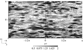
In § 4.1 the region in proximity of the leading edge is analysed, where due to the abrupt change of boundary conditions, non-equilibrium effects are the strongest. Particular attention is devoted to the velocity profiles and to the momentum balance, which, at  $x/\delta \approx 0$, are significantly perturbed by the temperature gradient. Figure 6, for instance, shows some instantaneous contours of the wall shear stress near the leading edge. Observe how the contours are condensed around
 $x/\delta = 0$ to the point that the interface becomes clearly visible, signalling a discontinuity.
Leading edge effects. Contours of wall shear stress ( $\tau _w$) near the leading edge of the isothermal wall. Values are non-dimensionalised with respect to
 $\overline {\tau }_w$, averaged over the surface of the wall.

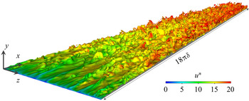
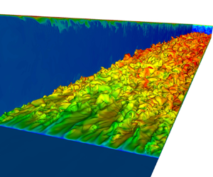
In § 4.2 the gradual development of the thermal boundary layer is investigated. Along the isothermal wall, the edge of the growing thermal layer (of which an instantaneous visualisation is given in figure 7) is at a non-equilibrium state. Yet, in a more inner region, a sublayer can be identified, where several quantities are equilibrated. The notion of equilibrium and non-equilibrium layers are clarified in this section, and a definition based on the mean energy balance is proposed.
Instantaneous iso-temperature  $\theta = (T - \bar {T}_{in} )/( T_w - \bar {T}_{in} ) = 0.9$ along the channel, coloured by the friction velocity
 $u^*$.

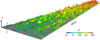
However, the analysis of § 4.2 is effectuated in a mean sense and, therefore, the findings concerning the equilibrium sublayer need to be contrasted to the evolution of several turbulent quantities. This is done in § 4.3, where the behaviour of the fluctuating temperature (of which an instantaneous field is provided in figure 8), turbulent heat flux and turbulent Prandtl number is investigated.
Instantaneous isosurface of fluctuating temperature  $(T^*)' = | T^* - \bar {T}^* | / T_{\tau } = 2$, coloured by the friction velocity
 $u^*$.

In the following, the same notation of § 3 is used.
4.1. Analysis of the leading edge
The abrupt change of boundary conditions taking place at  $x/\delta = 0$ generates enduring non-equilibrium effects which, as will be seen more in detail in § 4.2, do not vanish completely even at the distance of
 $x/\delta = 18{\rm \pi}$. However, there is a portion of the channel where these effects are so strong that the flow has a behaviour of its own that needs to be carefully investigated. This region is the leading edge, where the temperature gradient is the most elevated, as a consequence of the sudden change of thermal wall conditions (see the evolution of
 $Nu$ and
 $B_q$ in figure 5). Since the temperature is treated as an active scalar in our simulation, an impact on the velocity fields and momentum balance is expected. On the other hand, in this region the thermal boundary layer is too thin for any appreciable phenomenon to be observed on the temperature.
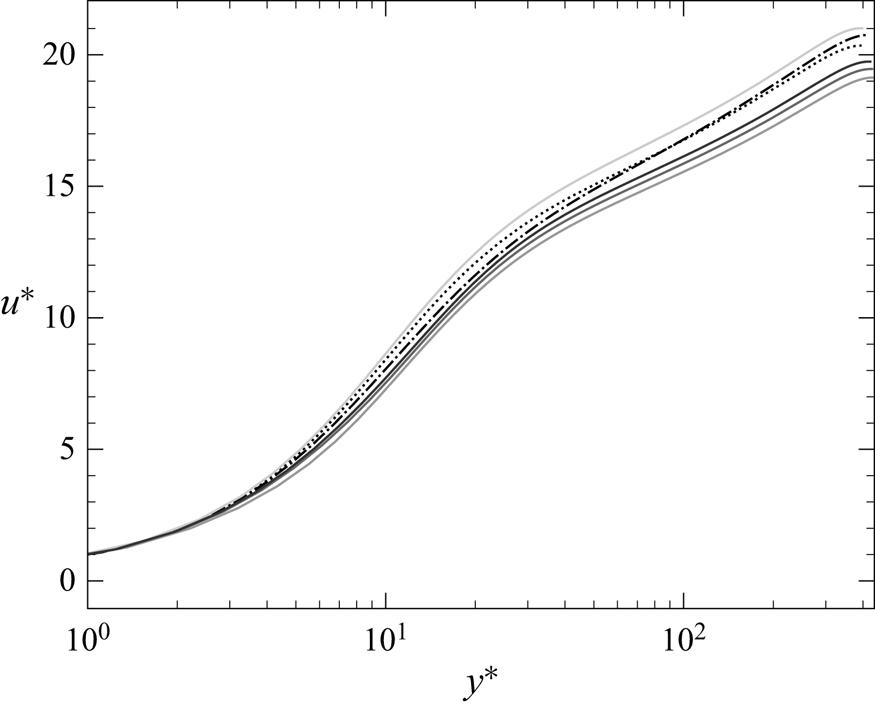
Figure 9 shows the mean streamwise velocity for  $x/\delta$ ranging between
 $[-0.06, 0.18]$ compared with the canonical profiles seen in § 3. Even if semi-local scaling is used, none of the profiles agree with the equilibrium ones, showing that, at these close distances from the leading edge, the perturbation cannot be ascribed to the only variation of mean fluid properties. This is particularly true for the profile at
 $x/\delta = 0.015$, for which the velocity boundary layer seems to be at equilibrium only for
 $y^* \lesssim 2$, i.e. in the viscous sublayer. The discrepancy of the profile at
 $x/\delta = - 0.06$ with respect to the equilibrium profile of § 3.1, instead, shows how the perturbation slightly propagates upstream.


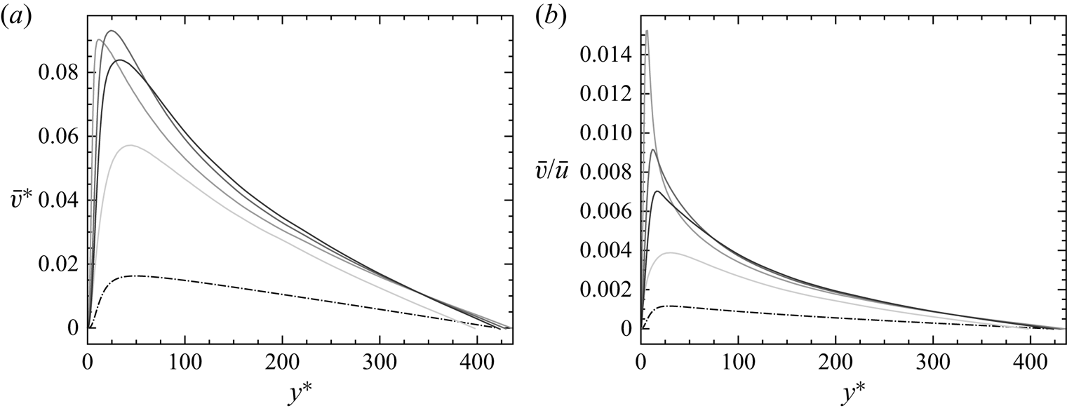
A similar impact on the streamwise velocity has been observed by Sanchez et al. (Reference Sanchez, Aulery, Toutant and Françoise2014) with a higher  $B_q$, arguing that the perturbation should be ascribed to the increase of the wall-normal velocity induced by the temperature gradient. It is certainly true that the wall-normal velocity considerably increases near the leading edge, as it can be seen in figure 10. Yet, the wall-normal velocity is also important at
 $x/\delta = - 0.06$, and, above all, always greater than zero. If the wall-normal velocity were only responsible for the deviation of the streamwise velocity, the impact would be expected to be similar to the one observed downstream of the leading edge, where the normal velocity is also always positive and of the same order of magnitude. Instead, as can be seen in figure 9, it is not the case, since an upper and lower shift is respectively observed at
 $x/\delta = -0.06$ and, for example,
 $x/\delta = 0.18$.
Wall-normal velocity profile for different  $x/\delta$ in semi-local scaling (a) and normalised with the mean streamwise velocity (b): ____ present results at
 $x/\delta = 0.015$, 0.18, 0.73 (from lightest to darkest); –
 $\cdot$ –
 $\cdot$ – equilibrium profile.

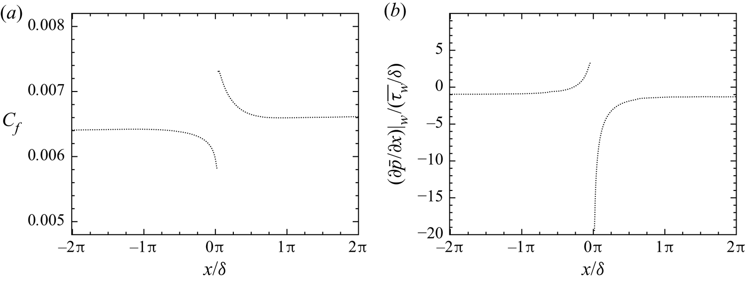
Hence, we propose a different interpretation, i.e. that the destabilisation of the boundary layer is due to the abrupt variation of the wall shear stress. Figure 11(a) shows the evolution of the skin friction coefficient  $C_f = \overline {\tau _w} / ( \frac {1}{2} \rho _b u_b^2 )$, where
 $\rho _b$ and
 $u_b$ are respectively the bulk density and the bulk velocity. At
 $x/\delta = 0^+$, the skin friction coefficient is at its maximum, which can be explained by the abrupt increase of the fluid dynamic viscosity at the leading edge of the isothermal wall. Then, the following relaxation and adaptation of the velocity gradient at the wall to the increased viscosity, leads to a quickly decreasing
 $C_f$ until it attains a plateau. At
 $x/\delta = 0^-$, instead, the skin friction coefficient is at its minimum. This is due to the fact that the flow, being subsonic, perceives the upcoming isothermal wall, and adapts by decreasing the gradient of streamwise velocity at the wall, while the dynamic viscosity remains constant since the wall is adiabatic. This perturbation, limited to a very small portion of the channel flow between
 $x/\delta \in [-1/2{\rm \pi}, 1/2{\rm \pi} ]$, results in a local perturbation of the wall streamwise pressure gradient, as can be seen in figure 11(b). While
 $({\partial \bar {p}}/{\partial x})|_w / ({\overline {\tau _w}}/{\delta }) \approx -1$ far from the leading edge, a positive (and, thus, adverse) and strongly negative (and, thus, favourable) pressure gradient is observed at
 $x/\delta = 0^-$ and
 $x/\delta = 0^+$, respectively.
Skin friction coefficient  $C_f$ (a) and non-dimensionalised wall pressure gradient (b) along the channel flow.

In order to take the effect of the streamwise pressure gradient into account, we introduce, following Simpson (Reference Simpson1983), the velocity scale  $u_p$ defined as
 \begin{equation} u_p = \left|\left.\frac{\mu}{\rho^2} \frac{\partial p}{\partial x}\right|_w \right|^{{1}/{3}}, \end{equation}
which, combined with the classic friction velocity  $u_{\tau } = | \tau _w / \rho |^{{1}/{2}}$, gives as proposed by Manhart, Peller & Brun (Reference Manhart, Peller and Brun2008),
 \begin{equation} u_{\tau p} = \sqrt{u_{\tau}^2 + u_{p}^2} . \end{equation}
We propose here a slight modification of this definition, which distinguishes positive and negative pressure gradients,
 \begin{equation} u_{\tau p} = \sqrt{u_{\tau}^2 + \rm{sign} \left( \left.\frac{\partial p}{\partial x}\right|_w \right)u_{p}^2} . \end{equation}
In this manner, the decrease of  $u_{\tau }$ in case of an adverse pressure gradient, and its increase in case of a favourable pressure gradient, are compensated by
 $u_p$, correcting the upward and downward deviation of the streamwise velocity at
 $x/\delta = 0^-$ and
 $x/\delta = 0^+$, respectively.
We can thus introduce the wall scaling
 \begin{equation} y^*_{\tau p} = \frac{y u_{\tau p}}{\nu}, \quad u^*_{\tau p} = \frac{u}{u_{\tau p}} , \end{equation}
where, analogously to semi-local scaling, fluid properties depend on the wall-normal direction in order to take the effect of the temperature gradient into account.
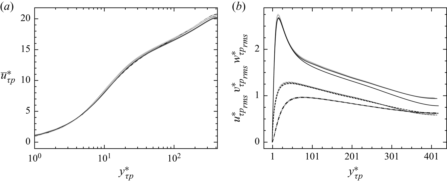
Figure 12(a) shows the same velocity profiles of figure 9 in the newly introduced wall scaling, while figure 12(b) illustrates the r.m.s. velocity profiles. Very good agreement is obtained between the different profiles in every region of the boundary layer, with the only exception of the r.m.s. streamwise velocity, for which the upward shift in the log layer has in any case to be ascribed to what is explained in § 3.2.
Mean streamwise velocity profile for different  $x/\delta$ in the newly introduced wall scaling (a). See figure 9 for a reference to lines and colours. Profiles of r.m.s. streamwise, wall-normal and spanwise velocities, respectively (b): ____, –
 $\cdot$ –
 $\cdot$ – and - - - - present results at
 $x/\delta = -0.06$, 0.015, 0.09, 0.18 and equilibrium (see § 3).

The fact that the velocity profiles are corrected by adopting a different wall scaling, suggests that, in our case, the perturbation is confined in the near-wall region and does not propagate towards the core of the flow. In the most general case, however, the leading edge effects are expected to become more important as  $B_q$ increases, with, in particular, larger wall-normal velocities and stronger variations of the pressure gradient. In these conditions, a modified wall scaling might not suffice to correct these effects.
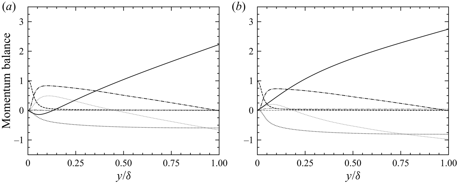
In order to corroborate our interpretation of the leading edge perturbations, the evolution of the different contributions to the momentum balance is analysed. For every crosswise section, integrating along the wall-normal direction the streamwise momentum balance yields
 \begin{align} \bar{\tau}_w(x) & ={-} \underbrace{\int_0^y \left(\bar{\rho} \tilde{u}\frac{\partial \tilde{u}}{\partial x}\right) \mathrm{d} y}_{I_x} - \underbrace{\int_0^y \left(\bar{\rho} \tilde{v}\frac{\partial \tilde{u} }{\partial y}\right) \mathrm{d} y}_{I_y} - \underbrace{\int_0^y \left( \frac{\partial \bar{p}}{\partial x}\right) \mathrm{d} y}_{II} \nonumber\\ &\quad + \underbrace{\int_0^y \left ( \frac{\partial \overline{\boldsymbol{\tau}_{xx}}}{\partial x}\right) \mathrm{d} y}_{III_x} + \underbrace{\overline{\boldsymbol{\tau}_{xy}}(y)}_{III_y} - \underbrace{\int_0^y \left(\frac{\partial }{\partial x}(\bar{\rho} \widetilde{u''u''} )\right)\mathrm{d} y}_{IV_x} - \underbrace{\bar{\rho} \widetilde{u''v''}(y)}_{IV_y} , \end{align}
where on the right-hand side of the equation there are two mean convective terms ( $I_x$ and
 $I_y$), the pressure gradient (
 $II$), two viscous terms (
 $III_x$ and
 $III_y$) and two terms associated with turbulent transport (
 $IV_x$ and
 $IV_y$). Figure 13 shows the different terms non-dimensionalised with respect to the average local wall shear stress
 $\overline {\tau _w}$ as a function of
 $y/\delta$ for two values of
 $x/\delta$, slightly upstream and downstream of
 $x/\delta = 0$.
Momentum flux balance at  $x/\delta = -0.06$ (a) and
 $0.18$ (b): ____ pressure gradient; - - - - streamwise (grey) and wall-normal (black) viscous terms;
 $\cdots \cdots$ streamwise (grey) and wall-normal (black) mean convective terms; –
 $\cdot$ –
 $\cdot$ – streamwise (grey) and wall-normal (black) turbulent terms.

Figure 13(a) is relative to  $x/\delta = -0.06$. At this close distance from the leading edge, the terms of (4.5) are strongly perturbed. The pressure gradient flux does not follow a straight line, showing that
 $\partial \bar {p} / \partial x$ is not uniform along the wall-normal direction and that the pressure field is bidimensional; it is also evident how the streamwise pressure gradient is positive (and, thus, adverse) until
 $y/\delta \approx 0.05$. Both mean convective terms are important; note the positive slope of the streamwise convective term near the wall, indicating that
 $\partial \tilde {u} / \partial x$ is negative and resulting in the aforementioned decrease of
 $\tau _w$. The remaining terms seem not to be significantly modified, indicating that the perturbation of the pressure gradient is fully compensated by the two convective terms. This is in agreement with the hypothesis that the non-equilibrium contributions to the momentum balance tend to self-compensate (see Larsson et al. Reference Larsson, Kawai, Bodart and Bermejo-Moreno2016).
Figure 13(b) is relative to  $x/\delta = 0.18$. The pressure gradient flux still does not follow a straight line and the pressure field is thus two dimensional; the positive slope of the pressure gradient term indicates that
 $\partial \bar {p} / \partial x$ is now negative for every
 $y / \delta$. Both mean convective terms are still important; near the wall, like at
 $x/\delta = -0.06$,
 $\partial \tilde {u} / \partial x < 0$, indicating that
 $\tau _w$ is decreasing. The perturbation of the momentum fluxes becomes negligible at
 $x/\delta \approx {\rm \pi}/2$, and completely disappears by
 $x/\delta \approx 3{\rm \pi}$, where the canonic momentum fluxes are finally retrieved, and the effects of the leading edge can be considered fully dissipated (not shown here).
Note that the results described in this section can only be observed if the temperature is handled as an active scalar, i.e. if the momentum and energy equations are coupled.
4.2. Identification of an equilibrium sublayer
Observe the behaviour of the instantaneous temperature isosurface illustrated in figure 7. Near the leading edge of the isothermal wall, the thermal layer is extremely thin, and the heated pockets are entirely located in the purely shear region of the flow. As the distance increases, these pockets thicken, breach through the viscous region and gradually become turbulent, until a fully developed state is attained at the outlet. The goal of this section is to describe the development of the thermal boundary layer from the leading edge to the outlet, and to identify, thanks to the mean energy balance, the different non-equilibrium regions of the flow.
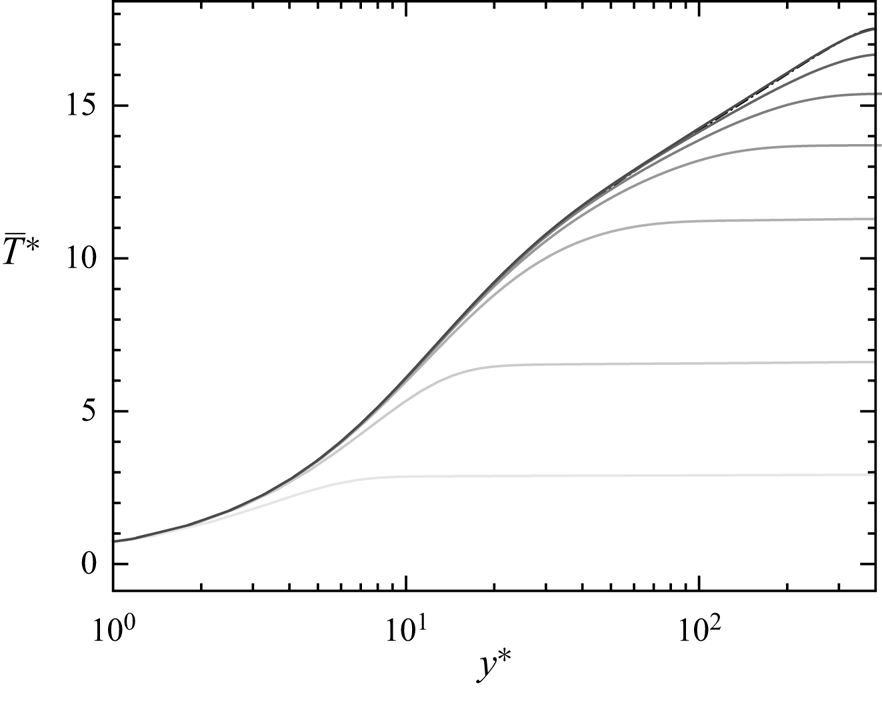
The progressive development of the thermal boundary layer is shown in figure 14, where several mean temperature profiles are plotted at different  $x/\delta$, and compared with the equilibrium profile of § 3.2. For every
 $x/\delta$, three distinct parts of the developing thermal boundary layer can be clearly identified. The first is the near-wall region where, for
 $y^* \in [0, h_{eq}^*]$, where
 $h_{eq}^*$ depends on and increases with
 $x/\delta$, the thermal boundary layer is fully developed and the mean temperature profile agrees with the one at equilibrium; note that this equilibrated behaviour is visible even at
 $x/\delta = 0.015$, where the leading edge effects described in § 4.1 are very much present. The second, for
 $y^* \in [h_{n-eq}^*, \delta ^{*}]$, where
 $h_{n-eq}^*$ also increases with
 $x/\delta$, is a region that is still not affected by the isothermal wall and the temperature profile is flat. The third, for
 $y^{*} \in [h_{eq}^{*}, h_{n-eq}^{*}]$, is instead the actual non-equilibrium developing portion of the thermal boundary layer, where the mean temperature profile is neither flat nor agreeing with the equilibrium one. As
 $x/\delta$ increases, both
 $h_{eq}^{*}$ and
 $h_{n-eq}^{*}$ tend towards the mid-height of the channel
 $\delta ^{*}$, and the non-equilibrium region disappears.
Profiles of mean temperature for different  $x/\delta$: ____ present results at
 $x/\delta = 0.015$, 0.21,
 $\frac {1}{2}{\rm \pi}$,
 $\frac {3}{2}{\rm \pi}$,
 $3.6{\rm \pi}$,
 $7.75{\rm \pi}$,
 $17.9{\rm \pi}$ (from lighter to darker); –
 $\cdot$ –
 $\cdot$ – equilibrium profile of § 3.2.

The existence of an equilibrium region in the development of the thermal boundary layer has been shown experimentally, for example, by Blom (Reference Blom1970) (who called this zone the adapted region) or Teitel & Antonia (Reference Teitel and Antonia1993). The objective is to analyse the evolution of the equilibrium layer (delimited by  $h_{eq}^{*}$) and of the non-equilibrium region (delimited by
 $h_{n-eq}^{*}$), yet it is first necessary to quantitatively define the notions of equilibrium and non-equilibrium.
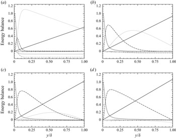
We propose to do so through the analysis of the different terms of the energy balance. The integration along the wall-normal direction of the local averaged energy equation gives a local heat budget for every crosswise section, i.e.
 \begin{align} \bar{q}_w(x) & = \underbrace{\int_0^y \left ( \bar{\rho} \tilde{u}\frac{\partial \tilde{h}}{\partial x} \right) \mathrm{d} y}_{I_x} + \underbrace{\int_0^y \left ( \bar{\rho} \tilde{v} \frac{\partial\tilde{h}}{\partial y} \right) \mathrm{d} y}_{I_y} + \underbrace{ \int_0^y \left( \frac{\partial \overline{q_x^{cd}}}{\partial x} \right) \mathrm{d} y}_{II_x} + \underbrace{ q_y^{cd}}_{II_y} \nonumber\\ &\quad + \underbrace{\int_0^y \left ( \frac{\partial }{\partial x} ( \bar{\rho} \widetilde{u''h''} ) \right) \mathrm{d} y}_{III_x} + \underbrace{\bar{\rho} \widetilde{v''h''}}_{III_y} - \underbrace{\int_0^y \left ( \frac{\mathrm{D} \bar{p}}{\mathrm{D} t} + \overline{\boldsymbol{\tau} : \nabla \boldsymbol{v} } \right)\mathrm{d} y}_{IV} - \underbrace{y S_{ener}}_{V} , \end{align}
where on the right-hand side of the equation there are two mean convective terms ( $I_x$ and
 $I_y$), two mean conductive terms (
 $II_x$ and
 $II_y$), two terms associated with turbulent heat transport (
 $III_x$ and
 $III_y$), one flux combining compressibility effects (
 $IV$) and the source term contribution (
 $V$). The evolution of these terms, normalised by
 $\bar {q}_w$, is shown for several
 $x/\delta$ in figure 15.
Energy flux balance at  $x/\delta = 0.73$ (a),
 $2{\rm \pi}$ (b),
 $5.7{\rm \pi}$ (c) and
 $16.5{\rm \pi}$ (d): ____ source term; - - - - streamwise (grey) and wall-normal (black) conductive fluxes;
 $\cdots \cdots$ streamwise (grey) and wall-normal (black) convective fluxes; –
 $\cdot$ –
 $\cdot$ – streamwise (grey) and wall-normal (black) turbulent fluxes; –
 $\cdot$
 $\cdot$ – compressibility effects.

Figures 15(a) and 15(b) are relative to  $x/\delta = 0.73$ and
 $x/\delta = 2{\rm \pi}$, respectively. At these short distances from the leading edge, many contributions which do not appear in equilibrium channel flows, are important. It is the case, for example, of the wall-normal convective flux since, as illustrated in figure 10, the mean vertical velocity is considerably higher compared with equilibrium. It is also the case of the streamwise turbulent flux, indicating that the correlation
 $\widetilde {u''h''}$ is evolving and increasing (in module). Yet, the preponderant contribution is that of the streamwise convective flux. Its positive slope near the wall indicates that the thermal boundary layer is developing and, as can be seen, the wall-normal conductive and turbulent fluxes are active. Farther away from the wall, its slope is negative and linear; since all the other contributions are constant, it is evident that the only active phenomenon is the uniform cooling caused by the source term. It is thus a portion of the boundary layer which still has not perceived the presence of the heated wall.
Further away from the leading edge, the canonic heat fluxes are gradually retrieved. At  $x/\delta = 5.7{\rm \pi}$ (see figure 15c),
 $\bar {\rho }\widetilde {v''h''} > 0$ everywhere but at
 $y/\delta = 1$, suggesting that the impact of the heated wall has by now reached the centre of the channel. At
 $x/\delta = 16.5{\rm \pi}$ (see figure 15d), the thermal boundary layer seems to be at equilibrium. However, notice how at
 $y/\delta \approx 1$ the streamwise convective flux is negative and decreasing, indicating that the temperature at the centre of the channel is still cooling under the action of the source term. This signals that even at the outlet the thermal boundary layer is not perfectly developed, given the limited extent of the simulated channel.
The evolution of the different contributions to the energy balance shows that the fluxes can be divided into two categories. The former is that of the equilibrium terms, which tend to become more and more important with  $x/\delta$ until stabilisation. The contributions that belong to this category are the wall-normal conductive flux and the wall-normal turbulent flux, which, summed, form the mean equilibrium flux
 $q^{eq}$. The latter is that of the non-equilibrium terms which, even if potentially preponderant near the leading edge, tend to become negligible and disappear with
 $x/\delta$. The contributions belonging to this category are the streamwise and wall-normal convective terms as well as the streamwise turbulent flux, which form the mean non-equilibrium flux
 $q^{n-eq}$. The remaining contributions, at least in the present case, are always negligible.
Now, defining the average total heat flux  $q^{tot}$ as
 \begin{equation} q^{tot} = \overline{q_w}(x) + y S_{ener} , \end{equation}
(4.6) can be rearranged in the form
 \begin{equation} q^{tot} = q^{eq} + q^{n-eq} , \end{equation}
where the compressibility effects and the streamwise conductive flux have been neglected. For every  $x/\delta$ and
 $y/\delta$, it is thus possible to define the ratio
 \begin{equation} R^{n-eq}_{tot} = \frac{| q^{n-eq} |}{| q^{eq} | + | q^{n-eq}|}, \end{equation}
quantifying the importance of the non-equilibrium terms in the energy balance.
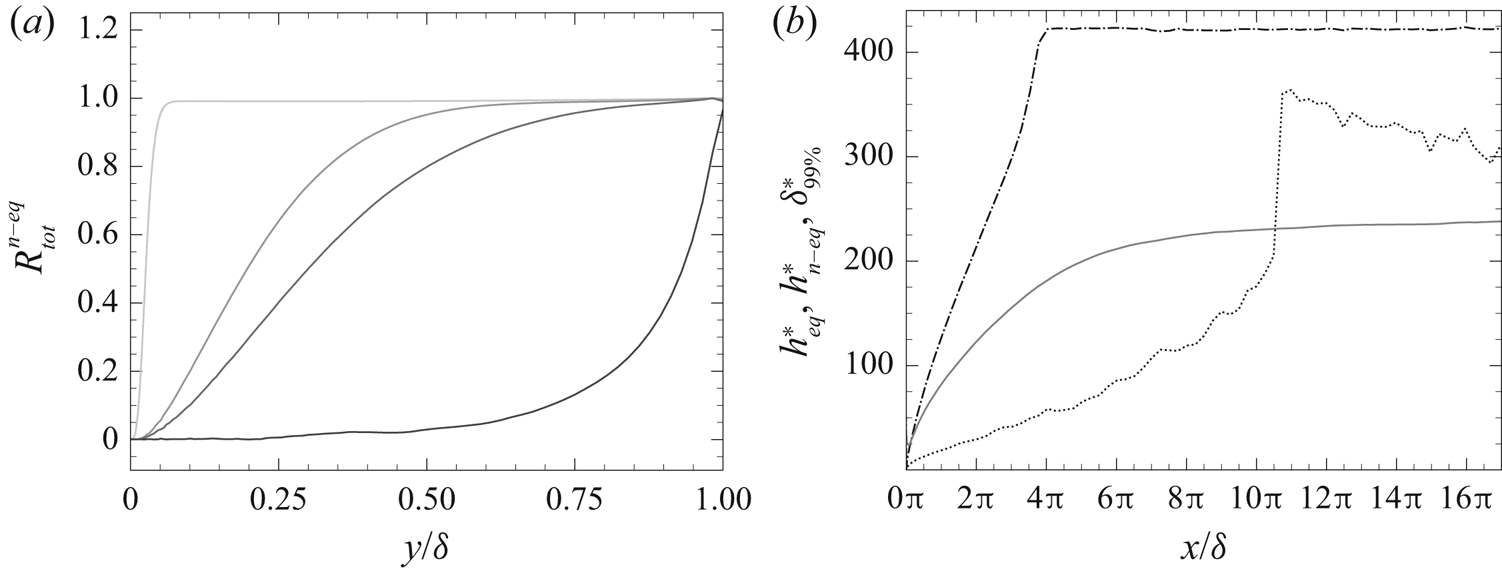
Figure 16(a) shows the evolution of  $R^{n-eq}_{tot}$ along the wall-normal direction for different
 $x/\delta$. The ratio
 $R^{n-eq}_{tot}$ allows us to define a quantitative criterion for distinguishing the three aforementioned regions of the developing thermal boundary layer. Indeed, as can be seen in figure 16(a), for every
 $x/\delta$, there is a near-wall portion of the boundary layer where the equilibrium fluxes are predominant with respect to the non-equilibrium ones; consequently,
 $R^{n-eq}_{tot} \approx 0$ and the energy equation can be simply approximated as
 \begin{equation} \overline{q_w} + y S_{ener} \approx q_y^{cd} + \bar{\rho} \widetilde{v''h''} . \end{equation}
The equilibrium region of the boundary layer, delimited by  $h^*_{eq}(x)$, can thus be defined as the region laying beneath an isoline of
 $R^{n-eq}_{tot}$ in the
 $x$–
 $y$ plane, for example,
 $R^{n-eq}_{tot} = 0.1$. For every
 $x/\delta$, there is also a portion of the boundary layer adjacent to the centre of the channel, where the non-equilibrium terms are predominant; consequently,
 ${R^{n-eq}_{tot} \approx 1}$, the only active physical phenomenon is the cooling caused by the source term and the mean temperature profile is flat along the wall-normal direction. This region of the boundary layer, delimited by
 $h^*_{n-eq}(x)$, can thus be defined as the region laying above an isoline of
 $R^{n-eq}_{tot}$, for example,
 $R^{n-eq}_{tot} = 0.9$. Finally, for every
 $x/\delta$ and for
 $y^* \in [h^{*}_{eq}, h^{*}_{n-eq}]$, the equilibrium and non-equilibrium fluxes are of the same order of magnitude, and the thermal boundary layer is in development.
Evolution of  $R^{n-eq}_{tot}$ with respect to
 $y/\delta$ for
 $x/\delta = 0.18$,
 $1.5{\rm \pi}$,
 $2.5{\rm \pi}$ and
 $16.5{\rm \pi}$ (from light grey to black) (a). Evolution of
 $h^*_{eq}$,
 $h^*_{n-eq}$ and
 $\delta ^*_{99\,\%}$ along the channel flow:
 $\cdots \cdots$
 $h^*_{eq}$; –
 $\cdot$ –
 $\cdot$ –
 $h^{*}_{n-eq}$; ____
 $\delta ^*_{99\,\%}$ (b).

Figure 16(b) shows the evolution of  $h^*_{eq}$ (defined as the isoline
 $R^{n-eq}_{eq} = 0.1$) and
 $h^{*}_{n-eq}$ (defined as the isoline
 $R^{n-eq}_{eq} = 0.9$) compared with the wall-scaled thermal boundary layer thickness
 $\delta ^*_{99\,\%} := h^* \ : \ | T_w - \bar {T}(h^*) | / | T_w - \bar {T}_c(x) | = 0.99$ .
The isoline  $h^{*}_{n-eq}$ is defined by a very loose criterion on
 $R^{n-eq}_{tot}$. Therefore, the advance of
 $h^{*}_{n-eq}$ towards the centre of the channel can benefit from the slightest expansion of the wall-normal heat flux, which takes place in regions of the flow where heat transport is efficiently carried out by turbulence. Consequently, the region beyond
 $h^{*}_{n-eq}$ quickly decays and disappears before
 $x/\delta = 4{\rm \pi}$. Downstream of this crosswise section, the effect of the heated wall has reached the centre of the channel and, as shown in figure 14, the mean temperature profile is nowhere flat any more.
The isoline  $h^{*}_{eq}$, instead, is defined by a very stringent criterion on the development of the equilibrium terms. Therefore, its growth is initially driven by the slow development of the wall-normal conductive flux, which takes place in regions of the flow where heat transport is essentially carried out by diffusion. As
 $h^{*}_{eq}$ grows and reaches the most turbulent parts of the boundary layer, its expansion accelerates, and, as can be qualitatively seen in figure 16(b), at
 $x/\delta \approx 10{\rm \pi}$ its growth rate is similar to that of
 $h^{*}_{n-eq}$ at
 $x/\delta \approx 3{\rm \pi}$, where
 $h^{*}_{eq} \approx h^{*}_{n-eq} \approx 300$. However,
 $h^{*}_{eq}$ does not reach the centre of the channel, and attains a peak at
 $y^* \approx 350$ before slowly decreasing. The criterion
 $R^{n-eq}_{tot} = 0.1$ is thus so stringent that the slight cooling of the source term at the centre of the channel (recall figure 15d) becomes appreciable at a certain
 $x/\delta$. With a higher criterion for
 $h^{*}_{eq}$, the same behaviour of
 $h^{*}_{n-eq}$ would be observed. However, note that
 $h^{*}_{eq} > \delta ^*_{99\,\%}$, indicating that the equilibrium sublayer attains in any case an essentially temperature-homogeneous region.
The evolution of  $h^{*}_{eq}$ and
 $h^{*}_{n-eq}$ is understandably case dependent. However, note that their definition, based on
 $R_{tot}^{n-eq}$, is general and can be used in all cases. By computing or estimating the size of
 $h^{*}_{eq}$ and comparing it with respect to a characteristic length of a given flow configuration, one can thus quantify the importance of the non-equilibrium effects in the thermal boundary layer.
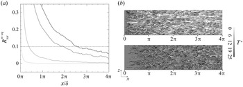
Finally, figure 17(a) shows the evolution of  $R_{tot}^{n-eq}$ as a function of
 $x/\delta$ for several wall distances. The intersection of every iso-
 $y^*$ with the isoline
 $R_{tot}^{n-eq} = 0.1$ can be seen as the non-equilibrium distance associated to that wall distance, i.e. the distance from the leading edge which is necessary for the thermal boundary layer to be at equilibrium between the wall and the specified
 $y^{*}$. Some contours of
 $T^*$ are given in figure 17(b) at
 $y^* = 12.5$ (above) and
 $y^* = 40$ (below). By comparing figure 17(a,b), one can appreciate the correspondence between the values of
 $R_{tot}^{n-eq}$ at these wall distances and the development of the heated turbulent structures as
 $x/\delta$ increases.
Evolution of  $R^{n-eq}_{tot}$ as a function of
 $x/\delta$ for several wall distances: ____
 $R^{n-eq}_{tot}$ for
 $y^* = 5$,
 $12.5$,
 $30$ and
 $40$ (from light grey to black, respectively); –
 $\cdot$ –
 $\cdot$ – isoline
 $R^{n-eq}_{tot} = 0.1$ (a). Instantaneous contours of temperature at
 $y^* = 12.5$ (above) and
 $y^* = 40$ (below) (b).

4.3. Development of turbulent heat transfer
The previous section has allowed us to appreciate and quantitatively define an equilibrium sublayer, where both the mean temperature and the mean energy balance are equilibrated. In this section we investigate its relevance with respect to the evolution along the isothermal wall of several turbulent quantities.
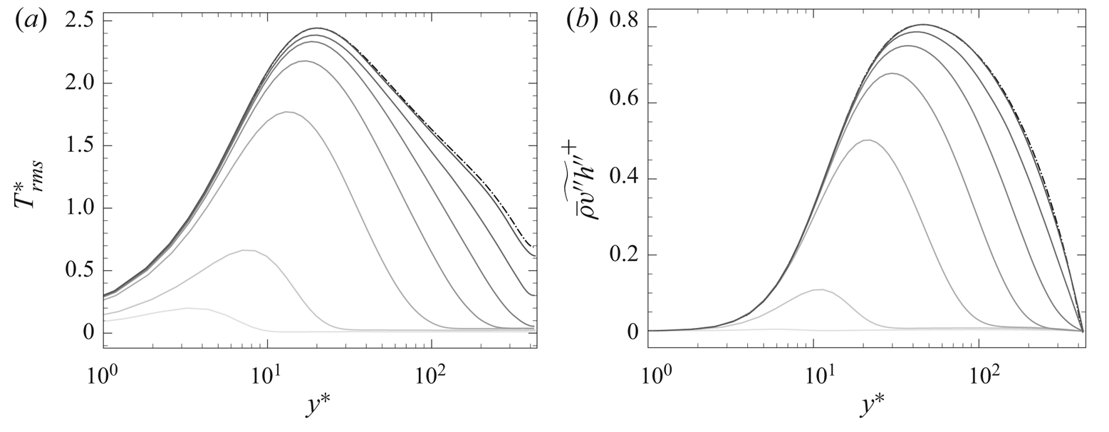
Figure 18 shows the evolution of the temperature fluctuations and of the wall-normal turbulent heat flux for different crosswise sections compared with equilibrium. Observe how both quantities progressively grow with  $x/\delta$, and how the peak shifts towards the higher
 $y^*$, until it stabilises at
 $y^* \approx 20$ for the r.m.s. temperature and
 $y^{*} \approx 45$ for the turbulent heat flux.
Profiles of r.m.s. temperature (a) and wall-normal turbulent heat flux (b) for different  $x/\delta$: ____ present results at
 $x/\delta = 0.015$, 0.21,
 $\frac {1}{2}{\rm \pi}$,
 $\frac {3}{2}{\rm \pi}$,
 $3.6{\rm \pi}$,
 $7.75{\rm \pi}$,
 $17.9{\rm \pi}$ (from lighter to darker); –
 $\cdot$ –
 $\cdot$ – equilibrium profiles of § 3.2.

The wall-normal turbulent heat flux (see figure 18b) clearly exhibits an equilibrated behaviour in the near-wall region for every  $x/\delta$. Interestingly, the same cannot be said about the fluctuating temperature (see figure 18a), which starts agreeing with equilibrium only at a certain distance from the leading edge (
 $x/\delta \approx 3/2{\rm \pi}$). This illustrates how the r.m.s. temperature has a stronger inertia, and needs a larger distance to settle, an aspect which has also been observed experimentally (see Teitel & Antonia Reference Teitel and Antonia1993). Also observe, in figure 8, the scant fluctuating structures near the leading edge. Figure 18(b) also outlines the fast wall-normal expansion of the turbulent heat flux during the early boundary layer development. As suggested in § 4.2, this explains the fast decay of the region
 $y^*>h^*_{n-eq}$ seen in figure 16(b).
The turbulent budgets of the enthalpy variance are now analysed. The time-averaged transport equation of  $\widetilde {h''^{2}}$ reads as (see, for a similar derivation, Vicquelin et al. Reference Vicquelin, Zhang, Gicquel and Taine2014)
 \begin{align} 0 & ={-}\underbrace{\frac{\partial }{\partial x} \left( \bar{\rho}\tilde{u} \frac{\widetilde{h''^2}}{2} \right)}_{I_x} -\underbrace{\frac{\partial }{\partial y} \left( \bar{\rho}\tilde{v} \frac{\widetilde{h''^2}}{2} \right)}_{I_y} -\underbrace{ \frac{\partial}{\partial x} ( \overline{q_x^{cd'}h'} )}_{II_x} -\underbrace{ \frac{\partial}{\partial y} ( \overline{q_y^{cd'}h'} )}_{II_y} \nonumber\\ &\quad + \underbrace{\overline{q_x^{cd'} \frac{\partial h'}{\partial x}} + \overline{q_y^{cd'} \frac{\partial h'}{\partial y}} + \overline{q_z^{cd'} \frac{\partial h'}{\partial z}}}_{III} + \underbrace{\overline{h'N'}}_{IV} -\underbrace{ \bar{\rho} \widetilde{u''h''} \frac{\partial \tilde{h}}{\partial x}}_{V_x} -\underbrace{\bar{\rho} \widetilde{v''h''} \frac{\partial \tilde{h}}{\partial y}}_{V_y} \nonumber\\ &\quad -\underbrace{\frac{1}{2} \frac{\partial}{\partial x} ( \bar{\rho} \widetilde{u''h''h''} )}_{VI_x} -\underbrace{\frac{1}{2} \frac{\partial}{\partial y} ( \bar{\rho} \widetilde{v''h''h''} )}_{VI_y} + \underbrace{\overline{h''} \left( - \frac{\partial \overline{q_x^{cd}}}{\partial x} - \frac{\partial \overline{q_y^{cd}}}{\partial y} + \overline{N} \right)}_{VII} , \end{align}
composed of the streamwise and wall-normal mean convective terms ( $I_x$ and
 $I_y$) and molecular diffusion (
 $II_x$ and
 $II_y$), molecular dissipation (
 $III$), a term of correlation between the enthalpy and
 $N$ (
 $IV$), where
 $N= ({\mathrm {D} p}/{\mathrm {D} t}) + \boldsymbol {\tau }_{ij} ({\partial u_i}/{\partial x_j}) + S_{ener}$ regroups the compressibility effects and the source term, the streamwise and wall-normal production (
 $V_x$ and
 $V_y$) and turbulent diffusion terms (
 $VI_x$ and
 $VI_y$), and, finally, a term related to the enthalpy–density correlation (
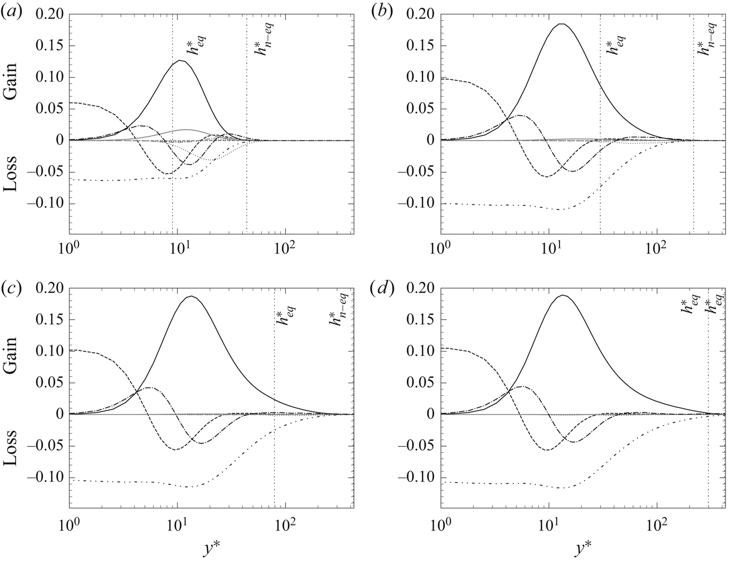
 $VII$). Figure 19 shows the evolution of the different terms (scaled with respect to
 $\overline {q_w}(x)^2/\overline {\mu _w}(x)$) for different crosswise sections. For each
 $x/\delta$, the values of
 $h^*_{eq}$ and
 $h^*_{n-eq}$ defined in § 4.2 are put into evidence. Some terms (
 $IV$ and
 $VII$), being always small and negligible, are not plotted. Finally, we have observed non-negligible levels of spurious numerical dissipation in our simulation, which has been added to the molecular dissipation (
 $III$) to yield a total dissipation term and a closed balance. The justification of this approach is given in supplementary materials B.
Budgets of enthalpy variance at  $x/\delta = 0.73$ (a),
 $2{\rm \pi}$ (b),
 $5.7{\rm \pi}$ (c) and
 $16.5{\rm \pi}$ : ____ streamwise (
 $V_x$: grey) and wall-normal (
 $V_y$: black) production; -
 $\cdot$
 $\cdot$ -
 $\cdot$
 $\cdot$ - molecular dissipation
 $III$; - - - - - streamwise (
 $II_x$: grey) and wall-normal (
 $II_y$: black) molecular diffusion; –
 $\cdot$ –
 $\cdot$ – streamwise (
 $VI_x$: grey) and wall-normal (
 $VI_y$: black) turbulent diffusion;
 $\cdots \cdots$ streamwise (
 $I_x$: grey) and wall-normal (
 $I_y$: black) mean convective terms.

Figure 19(a) is relative to  $x/\delta = 0.73$. At this close distance from the leading edge, the different terms of (4.11) are active only in a small portion (approximately
 $10\,\%$) of the boundary layer, delimited by
 $h^*_{n-eq}$, beyond which the flow is still not affected by the heated wall. Observe how it is between
 $h^*_{eq}$ and
 $h^*_{n-eq}$ that the non-equilibrium effects are located, with non-negligible streamwise convective and production terms. The classic contributions (wall-normal production, molecular dissipation and wall-normal turbulent and molecular diffusion), instead, appear to be under-developed. This is true even between the wall and
 $h^*_{eq}$, which is in agreement with the low level of r.m.s. temperature observed near the leading edge.
Figure 19(b) is relative to  $x/\delta = 2{\rm \pi}$. It is interesting to notice how all the streamwise non-equilibrium terms in the temperature variance budget have vanished. In the region between
 $h^*_{eq}$ and
 $h^*_{n-eq}$, while the mean energy balance presents strong non-equilibrium terms as seen in § 4.2, the enthalpy variance budget seems to merely feature the gradual development of the classic terms. Observe how in the equilibrium sublayer, instead, the different contributions controlling the r.m.s. temperature have by now settled, as can be seen by comparing figure 19(b–d) for
 $y^*< h^*_{eq}$. Accordingly, the r.m.s. temperature exhibits an equilibrated behaviour for
 $y^*< h^*_{eq}$ at these crosswise sections (see figure 18a).
Concerning the wall-normal turbulent heat flux, the time-averaged transport equation reads as (see, for a similar derivation, Vicquelin et al. Reference Vicquelin, Zhang, Gicquel and Taine2014)
 \begin{align} 0 & ={-}\underbrace{
\frac{\partial }{\partial x} ( \bar{\rho} \tilde{u}
\widetilde{v''h''} )}_{I_x} -\underbrace{ \frac{\partial
}{\partial y} ( \bar{\rho} \tilde{v}
\widetilde{v''h''})}_{I_y} + \underbrace{ \frac{\partial
}{\partial x} ( \overline{\tau_{2,1}'h'} -
\overline{q_x^{cd'}u'} )}_{II_x} +
\underbrace{\frac{\partial }{\partial y} (
\overline{\tau_{2,2}'h'} - \overline{q_y^{cd'}v'})}_{II_y}
\nonumber\\ & \quad -\underbrace{ \left (
\overline{\tau_{2,1}'\frac{\partial h'}{\partial x}} +
\overline{\tau_{2,2}'\frac{\partial h'}{\partial y}} +
\overline{\tau_{2,3}'\frac{\partial h'}{\partial z}} \right
) + \left ( \overline{q_x^{cd'} \frac{\partial v'}{\partial
x}} + \overline{q_y^{cd'} \frac{\partial v'}{\partial y}} +
\overline{q_z^{cd'} \frac{\partial v'}{\partial z}} \right
)}_{III} -\underbrace{ \overline{h'\frac{\partial
p'}{\partial y}}}_{IV} + \underbrace{\overline{v'N'}}_{V}
\nonumber\\ &\quad - \underbrace{ \bar{\rho}
\widetilde{u''h''} \frac{\partial \tilde{v}}{\partial x} -
\bar{\rho} \widetilde{u''v''} \frac{\partial
\tilde{h}}{\partial x}}_{VI_x} -\underbrace{ \bar{\rho}
\widetilde{v''h''} \frac{\partial \tilde{v}}{\partial y} -
\bar{\rho} \widetilde{v''v''} \frac{\partial
\tilde{h}}{\partial y}}_{VI_y} -\underbrace{ \frac{\partial
}{\partial x} ( \bar{\rho} \widetilde{u''v''h''} )}_{VII_x}
-\underbrace{ \frac{\partial }{\partial y} ( \bar{\rho}
\widetilde{v''v''h''} )}_{VII_y}\nonumber\\ &\quad +
\underbrace{\overline{h''} \left( - \frac{\partial
\bar{p}}{\partial y} + \frac{\partial
\overline{\tau_{2,1}}}{\partial x} + \frac{\partial
\overline{\tau_{2,2}}}{\partial y} \right) + \overline{v''}
\left ( \overline{N} - \frac{\partial
\overline{q_x^{cd'}}}{\partial x} - \frac{\partial
\overline{q_y^{cd'}}}{\partial y} \right )}_{VIII} ,
\end{align}
composed of the mean streamwise and wall-normal convective terms ( $I_x$ and
 $I_y$) and molecular diffusion (
 $II_x$ and
 $II_y$), the molecular dissipation (
 $III$), the enthalpy–pressure-gradient correlation (
 $IV$), the correlation between the wall-normal velocity and
 $N$ (
 $V$), the streamwise and wall-normal production (
 $VI_x$ and
 $VI_y$) and turbulent diffusion (
 $VII_x$ and
 $VII_y$), and, finally, two terms related to the enthalpy–density and wall-normal-velocity–density correlations (
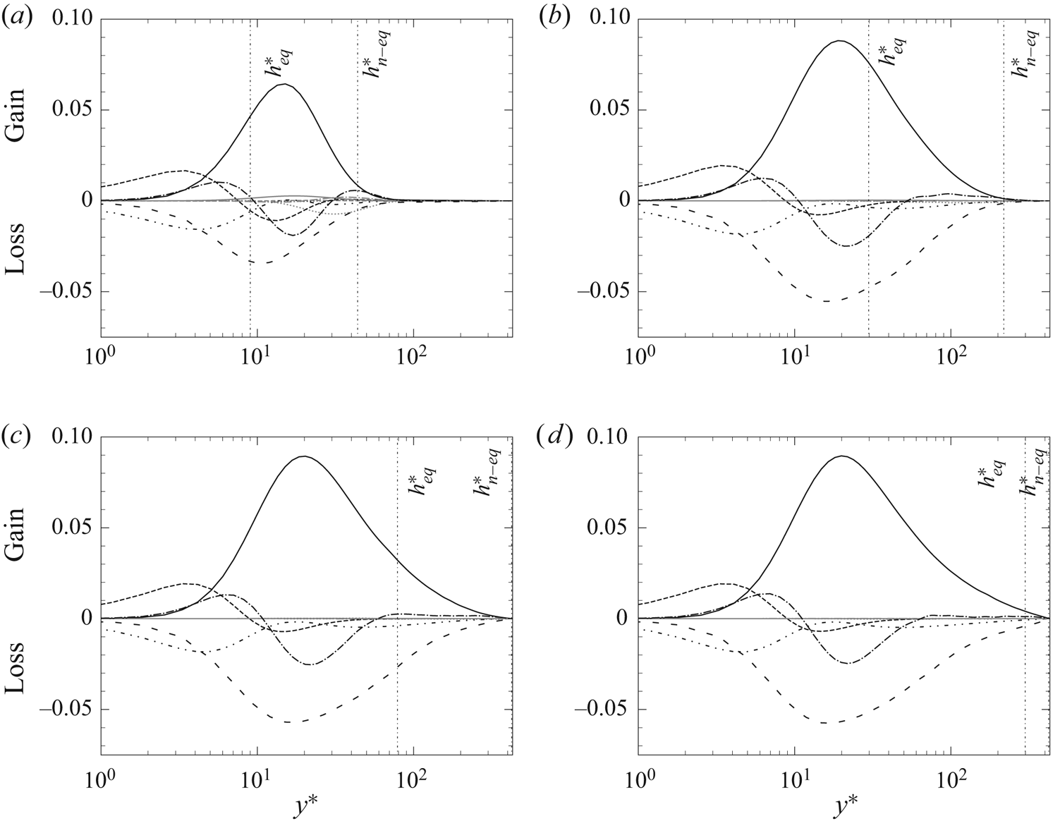
 $VIII$). Figure 20 shows the evolution of the different terms (scaled with respect to
 $\overline {q_w}(x) \overline {\tau _w}(x)/\overline {\mu _w}(x)$) for different crosswise sections with the respective
 $h^*_{eq}$ and
 $h^*_{n-eq}$ defined in § 4.2. The terms
 $V$ and
 $VIII$ are always small and negligible, and are not plotted.
Budgets of wall-normal turbulent heat flux at  $x/\delta = 0.73$ (a),
 $2{\rm \pi}$ (b),
 $5.7{\rm \pi}$ (c) and
 $16.5{\rm \pi}$: ____ streamwise (
 $VI_x$: grey) and wall-normal (
 $VI_y$: black) production; -
 $\cdot$
 $\cdot$ -
 $\cdot$
 $\cdot$ - molecular dissipation
 $III$; - - - - - streamwise (
 $II_x$: grey) and wall-normal (
 $II_y$: black) molecular diffusion; –
 $\cdot$ –
 $\cdot$ – streamwise (
 $VII_x$: grey) and wall-normal (
 $VII_y$: black) turbulent diffusion;
 $\cdots \cdots$ streamwise (
 $I_x$: grey) and wall-normal (
 $I_y$: black) convective terms; – – – – enthalpy–pressure-gradient correlation
 $IV$.

Most of the observations made concerning the budgets of enthalpy variance are still valid. The non-equilibrium region  $h^*_{eq} < y^* < h^*_{n-eq}$ manifests itself with a gradual development of the classic terms (including, in this case, the enthalpy–pressure-gradient), rather than with the presence of strong streamwise terms as seen in § 4.2 for the mean energy balance. In this case, the only streamwise terms that are important near the leading edge are the streamwise production and convection, as illustrated in figure 20(a). Yet, even these terms become negligible at
 $x/\delta = 2{\rm \pi}$ (see figure 20b).
The only difference with the enthalpy variance budget is the behaviour for  $y^*< h^*_{eq}$. For the wall-normal turbulent heat flux, the classic budgets have settled in the equilibrium sublayer even for the smallest
 $x/\delta$, which is in agreement with the equilibrated profiles observed for
 $y^*< h^*_{eq}$ in figure 18(b).
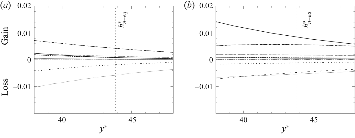
Figure 21 shows the details of the budgets of enthalpy variance and wall-normal turbulent heat flux for  $y^* \approx h^*_{n-eq}$ at
 $x/\delta = 0.73$, i.e. the same crosswise section of figures 19(a) and 20(a). In both figures 21(a) and 21(b), it can be seen how the turbulent diffusion plays an important role in the development of both
 $\widetilde {h''^{2}}$ and
 $\widetilde {v''h''}$. In the case of the enthalpy variance, turbulent diffusion is actually the only term inducing a gain of enthalpy fluctuations, mostly counterbalanced by the mean streamwise convective term. The presence of non-negligible turbulent diffusion around
 $y^* \approx h^*_{n-eq}$ corroborates the hypothesis formulated in § 4.2, i.e. that the fast decay of the temperature-homogeneous region beyond
 $y^* > h^*_{n-eq}$ might be due to the efficient heat transport carried out by turbulence.
Budgets of enthalpy variance (a) and wall-normal turbulent heat flux (b) at  $x/\delta = 0.73$ zoomed at
 $y^* \sim h^*_{n-eq}$. See figures 19 and 20 for the notation.

Finally, the behaviour of the turbulent Prandtl number  $Pr_t$ is investigated. The turbulent Prandtl number
 $Pr_t$ offers a simple way of relating the turbulent kinematic viscosity
 $\nu _t$ and conductivity
 $\lambda _t$ in Reynolds-averaged Navier–Stokes (RANS), LES or wall-modelled LES (WMLES) turbulence modelling, and, analogously to the molecular Prandtl number,
 $Pr_t$ is defined as
 \begin{equation} Pr_t = \frac{\bar{\rho} \nu_t \overline{c_p}}{\lambda_t} = \frac{-\bar{\rho}\widetilde{u''v''}}{-\bar{\rho}\widetilde{v''h''}/\overline{c_p}} \frac{\mathrm{d}\bar{T}/\mathrm{d} y}{\mathrm{d}\overline{u}/\mathrm{d} y} . \end{equation}
Experimentally, Blom (Reference Blom1970) analysed the evolution of the turbulent Prandtl number in a developing thermal boundary layer, and found that it varies in both wall-normal and streamwise directions, while suggesting that a universal distribution of  $Pr_t$ can only be expected in the near-wall region. Antonia et al. (Reference Antonia, Danh and Prabhu1977) carried out similar investigations, and found that the turbulent Prandtl number is generally of the order of magnitude of one, thus showing the overall validity of the Reynolds analogy; according to their experimental results, values of
 $Pr_t$ strongly exceeding unity can only be found near the leading edge of the thermal boundary layer.
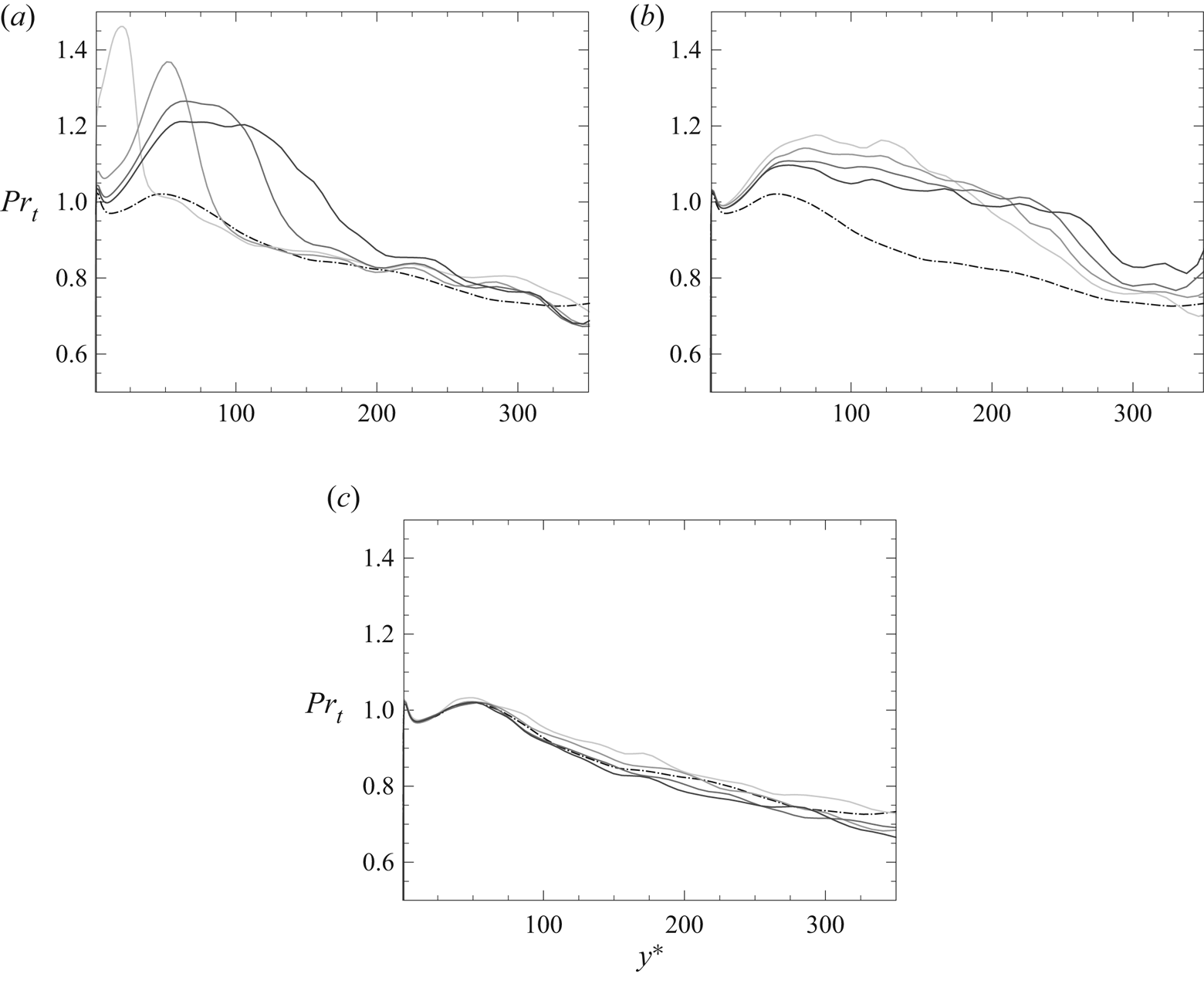
Figure 22 displays the evolution of  $Pr_t$ for different
 $x/\delta$, compared with its equilibrium profile. The latter is represented by the dashed-dotted line. It can be seen that
 $Pr_t$ is slightly greater than unity at the wall, before decreasing and attaining
 $Pr_t \approx 0.7$ in the channel core flow. Its mild gradient along the wall-normal direction can justify the use of a constant average turbulent Prandtl number (usually
 $Pr_t \approx 0.9$), at least in equilibrium boundary layers (see, for instance, Kawai & Larsson Reference Kawai and Larsson2012).
Evolution of turbulent Prandtl number in the wall-normal direction for different  $x/\delta$: ____ present results at (from light to dark grey)
 $x/\delta = 0.18$,
 $0.73$
 $0.5{\rm \pi}$ and
 $0.75{\rm \pi}$ (a), at
 $x/\delta = {\rm \pi}$,
 $1.25{\rm \pi}$,
 $1.5{\rm \pi}$ and
 $1.75{\rm \pi}$ (b); at
 $x/\delta = 5.67{\rm \pi}$,
 $8.25{\rm \pi}$,
 $10.8{\rm \pi}$ and
 $16.5{\rm \pi}$ (c); –
 $\cdot$ –
 $\cdot$ – equilibrium profile.

Figure 22(a) shows the evolution of  $Pr_t$ for four crosswise sections which are relatively close to the leading edge. As can be seen, the turbulent Prandtl number does not exhibit an equilibrated behaviour in the near-wall region, where its value largely exceeds unity. Since the turbulent viscosity and conductivity, on their part, are at equilibrium in the wall vicinity (not shown here), this behaviour is explained by the abrupt increase of
 $c_p$ astride
 $x/\delta = 0$, and represents another leading edge effect. Further away from
 $x/\delta = 0$,
 $Pr_t$ remains for the most part greater than unity and, as
 $x/\delta$ increases, its perturbation expands in the wall-normal direction, while its intensity decreases. This tendency is particularly evident in figure 22(b) for
 $x/\delta$ ranging between
 $[{\rm \pi}, 1.75{\rm \pi} ]$. The profiles of figure 22(c), instead, illustrate how the turbulent Prandtl number essentially returns to equilibrium at
 $x/\delta \approx 5{\rm \pi}$.
The larger values of  $Pr_t$ during the development of the thermal boundary layer are explained by the fact that its numerator,
 $\nu _t$, is already well established with the incoming fully developed adiabatic flow; its denominator
 $\lambda _t$, instead, is initially small, since heat transfer is essentially carried out by mean convection, as seen in § 4.2. The results are therefore in qualitative agreement with those of Antonia et al. (Reference Antonia, Danh and Prabhu1977). On the other hand, there is no evidence of the existence of a universal distribution in the near-wall region, as indicated in Blom (Reference Blom1970). It appears to be quite the opposite since the highest values of
 $Pr_t$ can be found near the leading edge in the very proximity of the wall.
5. Conclusion
The DNS of a non-equilibrium turbulent thermal boundary layer is performed in a channel flow. Non-equilibrium is induced by a step change in wall temperature, which perturbs a turbulent adiabatic flow initially at equilibrium. The flow later evolves towards a new equilibrium state, characterised by a fully developed thermal boundary layer. The simulation is performed under one single flow regime, in terms of Reynolds number, Mach number and heat flux parameter. The study throws light on several physical phenomena which are expected to appear in phenomenologically similar non-equilibrium flows where a streamwise and transverse development of the thermal boundary layer follows a sudden perturbation.
The leading edge of the isothermal wall appears to be the most perturbed region of the flow, with effects that also slightly propagate upstream. The temperature step change causes a discontinuity of the wall shear stress and of the pressure gradient, which modify the velocity profiles. In our case, these modifications seem to be fully corrected by the adoption of a new wall scaling, which takes into account both the mean fluid property variations and the pressure gradient. This suggests that the disturbance is confined in the very near-wall region, and does not propagate to the core of the flow. In the most general case, these effects are expected to appear at any discontinuity of thermal wall condition and, being regulated by the heat flux parameter  $B_q$, to expand and aggravate as
 $B_q$ increases, i.e. for stronger temperature gradients or lower friction velocities. In these conditions, one should anticipate larger wall-normal velocities and stronger pressure gradient discontinuities astride the leading edge, the effects of which might not be corrected by only adopting a different wall scaling.
The study has allowed for the identification of an equilibrium sublayer, where several quantities are equilibrated. These quantities are the mean temperature, the energy fluxes, the wall-normal turbulent heat flux and its budgets. Defined as the part of the flow where the equilibrium contributions to the energy balance are preponderant, the equilibrium region is initially confined in the conductive sublayer and slowly driven by heat diffusion, before it reaches the most turbulent part of the flow. The existence of such an equilibrium layer is an important assumption for turbulence modelling. It may a priori justify, for instance, the use of equilibrium wall models in the WMLES of non-canonic flows, as long as the modelled portion of the flow lays within the aforesaid equilibrium layer. Experimentally observed by several authors, there is reason to believe that it might be identifiable in any comparable non-equilibrium flow, where the same criterion on the energy balance contributions can be adopted to analyse it. However, stronger leading edge effects might initially disrupt its structure and delay its development.
Other quantities do not have the expected behaviour in the equilibrium sublayer. Low levels of temperature fluctuations, for instance, have been observed in the early development of the thermal boundary layer, accompanied by under-developed budgets of enthalpy variance. This illustrates the stronger inertia of the r.m.s. temperature, and it is an aspect that has also been observed experimentally. Finally, the turbulent Prandtl number exceeds unity in a relatively large portion of the flow, which includes part of the equilibrium sublayer. The perturbation is due to the fact that heat transfer is initially carried out by mean convection, and only to a minor extent by turbulence. An important role is also played by the abrupt variation of fluid properties at the beginning of the isothermal wall, thus representing another leading edge effect. Even in the present case, characterised by a mild temperature gradient, different models for the turbulent Prandtl number might be required to take into account its modified behaviour in RANS or LES modelling of turbulent heat transfer.
In perspective, further investigations are required to deepen our knowledge of heat transfer taking place in non-equilibrium turbulent flows. Different flow regimes, in terms of Reynolds number, Mach number and heat flux parameter, should allow for wider generalisations of the effects observed in this study, with a particular allusion to the leading edge perturbation and the evolution of the equilibrium sublayer. Entirely different non-equilibrium heat transfer cases, instead, could bring to light other physical phenomena that our flow configuration has not allowed us to observe. The predominant terms identified outside the equilibrium sublayer can be different in another kind of flow topology.
Supplementary material
Supplementary materials are available at https://doi.org/10.1017/jfm.2021.1104.
Acknowledgements
The numerical study was carried out thanks to the HPC resources of TTGC under the allocation 2018-A0042B10159 made by GENCI, and the HPC resources from the ‘Mésocentre’ computing centre of CentraleSupélec and École Normale Supérieure Paris-Saclay supported by CNRS and grants from Ministry of Research via the Contrat Plan État-Région.
Declaration of interests
The authors report no conflict of interest.