1. Introduction
Complex networks are often studied via mathematical analysis of null models that can match the network degree distribution. For scale-free networks, this degree distribution follows a power law. In many real-world networks, such as the Internet, social networks, and biological networks, the power-law exponent
 $\tau$
was found to be between 2 and 3 [Reference Albert, Jeong and Barabási1, Reference Faloutsos, Faloutsos and Faloutsos19, Reference Jeong, Tombor, Albert, Oltvai and Barabási30, Reference Vázquez, Pastor-Satorras and Vespignani43]. In such scale-free networks, high-degree vertices called hubs are likely present, and give rise to scale-free properties such as small distances and fast information spreading. The hubs also crucially influence local properties such as clustering [Reference van der Hofstad, Janssen, van Leeuwaarden and Stegehuis26, Reference Stegehuis, van der Hofstad, van Leeuwaarden and Janssen41] and the occurrence of subgraphs [Reference Ostilli36]. Clustering can be measured in terms of the probability c(k) that a degree-k vertex creates triangles. Both empirically [Reference Maslov, Sneppen and Zaliznyak33, Reference Pastor-Satorras, Vázquez and Vespignani38] and theoretically [Reference Colomer-de Simon and Boguñá17, Reference Stegehuis, van der Hofstad, van Leeuwaarden and Janssen41], it has been shown that c(k) falls off with k, and hence that hubs are less likely to take part in triangles.
Whereas triangles and even larger subgraphs require us to study the correlation between at least three vertices, in this paper we study the degree correlation between pairs of two vertices in terms of a(k), the average degree of a neighbour of a vertex of degree k. According to several studies [Reference Barabási2, Reference Catanzaro, Boguñá and Pastor-Satorras15], this degree–degree correlation is an essential local network property, because it also falls off with k and can largely explain the fall-off of c(k) [Reference Boguñá and Pastor-Satorras9, Reference Catanzaro, Boguñá and Pastor-Satorras15, Reference Serrano and Boguñá40]. We provide support for this statement by identifying an explicit relation between a(k) and c(k) for large k. But the main goal of this paper is to explain the full spectrum
 $k\mapsto a(k)$
for all k, and to provide theoretical underpinning for the widely observed a(k) fall-off.
There exists a vast array of papers, empirical, non-rigorous, and rigorous, on a(k) [Reference Barabási2, Reference Barrat, Barthélemy, Pastor-Satorras and Vespignani3, Reference Boguñá and Pastor-Satorras9, Reference Boguñá, Pastor-Satorras and Vespignani10, Reference Catanzaro, Boguñá and Pastor-Satorras15, Reference Mayo, Abdelzaher and Ghosh34, Reference Park and Newman37, Reference Pastor-Satorras, Vázquez and Vespignani38, Reference Vázquez42, Reference Yao, van der Hoorn and Litvak45]. The function
 $k\mapsto a(k)$
describes the correlation between the degrees on the two sides of an edge, and classifies the network into one of the following three categories [Reference Newman35]. When a(k) increases with k, the network is said to be assortative: vertices with high degrees mostly connect to other vertices with high degrees. When a(k) decreases in k, the network is said to be disassortative. Then high-degree vertices typically connect to low-degree vertices. When a(k) forms a flat curve in k, the network is said to be uncorrelated. In this case, the degrees on the two different sides of an edge can be viewed as independent of each other, a desirable property when studying the mathematical properties of networks. But the fact is that the majority of real-world networks with power-law degrees and unbounded degree fluctuations (
 $\tau\in(2,3)$
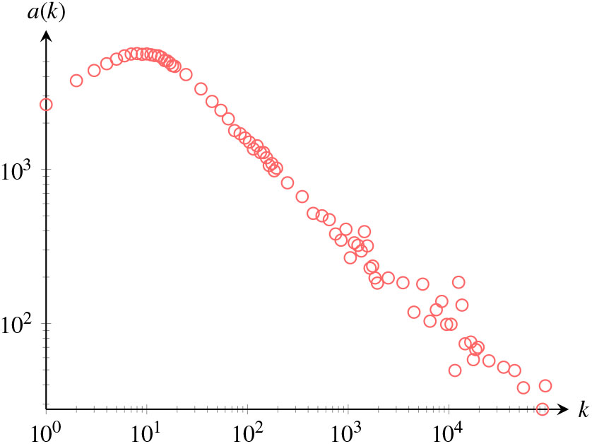
) show a clear decay of a(k) as k grows large [Reference Maslov, Sneppen and Zaliznyak33, Reference Pastor-Satorras, Vázquez and Vespignani38]. Figure 1 illustrates this for the YouTube friendship network [Reference Leskovec and Krevl32]. Hence, scale-free networks are inherently disassortative, and hubs are predominantly connected to small-degree vertices. In complex network theory, such a well-established empirical fact then asks for a theoretical explanation. Typically, this explanation comes in the form of a null model that matches the degree distribution and has the empirical observation as a property, in this case disassortivity, or more specifically, the essential features of the curve
 $k\mapsto a(k)$
.
a(k) for the YouTube friendship network [Reference Leskovec and Krevl32].

The popular configuration model [Reference Bollobás11] generates random networks with any prescribed degree distribution, but only results in uncorrelated networks when including self-loops and multi-edges. Hence, the configuration model can never explain the a(k) fall-off. We therefore resort to different null models that, contrary to the configuration model, generate random networks without self-loops and multi-edges. The resulting simple random networks are therefore prone to the structural correlations that come with the presence of hubs. We study a(k) for three widely used random graph models: the erased configuration model, the rank-1 inhomogeneous random graph (also called hidden variable model), and the hyperbolic random graph. We show that these models display universal a(k)-behaviour: For k sufficiently small, a(k) is independent of k. Thus, in simple scale-free networks, neighbours of small-degree vertices are similar. We then identify the value of k for which a(k) starts decaying. An intuitive explanation for the a(k) fall-off is that in simple networks, high-degree vertices have so many neighbours that they must reach out to lower-degree vertices, because networks typically only contain a small amount of high-degree vertices. This causes the average degree of a neighbour of a high-degree vertex to be smaller. Thus, single-edge constraints may cause the decay of a(k).
2. Main results
We first define the average nearest-neighbour degree a(k,G) of a graph G in more detail. Let
 $ (D_i)_{i\in [n]} $
be the degree sequence of the graph, where
 $[n]=1,\ldots,n$
. Furthermore, let
 $N_k$
denote the total number of degree k vertices in the graph, and let
 $\mathcal{N}_i$
denote the neighbourhood of vertex i. The average nearest-neighbour degree of graph G is then defined as
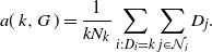 \begin{equation}a(\:k,G\:)=\frac{1}{k N_k}\sum_{i:D_i=k}\sum_{j\in\mathcal{N}_i}D_j.\end{equation}
Note that it is possible that no vertex of degree k exists in the graph, and in this situation we set
 $a(k,G)=0$
. We therefore analyse
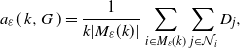 \begin{equation}a_\varepsilon(\:k,G\:)=\frac{1}{k|M_\varepsilon(k)|}\sum_{i\in M_\varepsilon(k)}\sum_{j\in\mathcal{N}_i}D_j,\end{equation}
where
 \[
M_\varepsilon(k)=\{i\in[n]\colon D_i\in[k(1-\varepsilon),k(1+\varepsilon)]\}.
\]
When
 $M_{\varepsilon}(k)=\emptyset$
, we set
 $a_\varepsilon(k,G)=0$
. We will show that in the models we analyse,
 $M_{\varepsilon}(k)$
is non-empty with high probability, so that
 $a_{\varepsilon}(k,G)$
is well-defined with high probability. Note that
 $a(k,G)=a_0(k,G)$
. We now analyse
 $a_\varepsilon(k,G)$
, first for the erased configuration model in Section 2.1 and then for the rank-1 inhomogeneous random graph and the hyperbolic random graph in Sections 2.3 and 2.4.
2.1. The erased configuration model
Given a positive integer n and a degree sequence
 $ (D_1,D_2,\ldots, D_n) $
such that the sum of the degrees is even, the configuration model is a (multi)graph where vertex i has degree
 $D_i$
[Reference Bollobás11]. We start with
 $D_j$
free half-edges adjacent to vertex j, for
 $j=1, \ldots, n$
. The configuration model is then constructed by pairing free half-edges uniformly at random into edges, until no free half-edges remain. Conditionally on obtaining a simple graph, the resulting graph is a uniform graph with the prescribed degrees. This is why the configuration model is often used as a null model for real-world networks with given degrees. When the degree distribution has an infinite second moment, however, the probability of obtaining a simple graph tends to zero as n grows large (see e.g. [Reference van der Hofstad23, Chapter 7]). In this setting the configuration model can no longer be used as a null model for simple real-world networks. The erased configuration model is the model where all multiple edges are merged and all self-loops are removed [Reference Britton, Deijfen and Martin-Löf13]. We take the original degree sequence to be an i.i.d. sample from the distribution
 \begin{equation}
{\mathbb{P}}(D=k)=c k^{-\tau} {,}
\end{equation}
where
 $\tau\in(2,3)$
so that
 ${\mathbb{E}}[D^2]=\infty$
. We denote
 ${{\mathbb{E}}[{D}]}=\mu$
. When this sample constructs a degree sequence such that the sum of the degrees is odd, we add an extra half-edge to the last vertex. This does not affect our computations. We denote the actual degree sequence of the graph after merging the multiple edges and removing self-loops by
 $ ({D^{{(er)}}})_{i\in[n]} $
, and we call these the resulting degrees.
2.1.1. Stable random variables
The limit theorem of
 $a(k,G_n)$
for the erased configuration model contains stable random variables. A random variable X follows a stable distribution if, for any positive numbers
 $a_1$
and
 $a_2$
, there exists a real number
 $b_1=b_1(a_1,a_2)$
and a positive number
 $b_2=b_2(a_1,a_2)$
such that
 \begin{equation} a_1X_1+a_2X_2\overset{d}{=}b_1+b_2X,\end{equation}
where
 $X_1$
and
 $X_2$
are independent copies of X. Stable random variables can be parametrized by four parameters, and are usually denoted by
 $\mathcal{S}_\alpha(\sigma,\beta,\mu)$
(see e.g. [Reference Whitt44, Chapter 4]). Throughout this paper, we will only use stable distributions with
 $\sigma=1,\beta=1,\mu=0$
and we denote
 $\mathcal{S}_\alpha=\mathcal{S}_\alpha(1,1,0)$
to ease notation.
We now state the main result for the erased configuration model.
Theorem 1. (a(k, G) in the erased configuration model.) Let
 $ (G_n)_{n\geq 1} $
be a sequence of erased configuration models on n vertices, where the degrees are an i.i.d. sample from (3). Take
 $\varepsilon_n=1/(\log(\log(n)))$
and let
 $\Gamma$
denote the gamma function.
(i) For
 $k \ll n^{(\tau-2)/(\tau-1)}/\log(n)$
,
(5)where\begin{equation}\frac{a_{\varepsilon_n}(k,G_n)}{n^{(3-\tau)/(\tau-1)}}{{\stackrel{d}{\longrightarrow}}} \frac{1}{\mu}\bigg(\frac{2c \Gamma(\frac{5}{2}-\frac{1}{2}\tau )}{ (\tau-1)(3-\tau)}\cos\bigg(\frac{\pi(\tau-1)}{4}\bigg)\bigg)^{2/(\tau-1)} \mathcal{S}_{(\tau-1)/2},\end{equation}
$\mathcal{S}_{(\tau-1)/2}$
is a stable random variable.
(ii) For
$ n^{(\tau-2)/(\tau-1)} \ll k \ll n^{1/(\tau-1)}/\log(n)$
,
(6)\begin{equation}\frac{a_{\varepsilon_n}(k,G_n)}{n^{3-\tau}k^{\tau-3}}{{\stackrel{{\mathbb{P}}}{\longrightarrow}}} -c \mu^{2-\tau}\Gamma(2-\tau).\end{equation}





Remark 1. The convergence in (5) also holds jointly in k and n, so that for fixed
 $m\geq 1$
and
 $1\leq k_1<k_2<\cdots <k_m \ll n^{(\tau-2)/(\tau-1)}/\log(n)$
,
 \begin{equation*}\frac{(a_{\varepsilon_n}(k_i,G_n))_{i\in[m]}}{n^{(3-\tau)/(\tau-1)}}{{\stackrel{d}{\longrightarrow}}} \frac{1}{\mu}\bigg(\frac{2c \Gamma(\frac{5}{2}-\frac{1}{2}\tau )}{ (\tau-1)(3-\tau)}\cos\bigg(\frac{\pi(\tau-1)}{4}\bigg)\bigg)^{2/(\tau-1)} \mathcal{S}_{(\tau-1)/2}\boldsymbol{1},\end{equation*}
where
 $\boldsymbol{1}\in\mathbb{R}^m$
is a vector with m entries equal to 1. Thus,
 $a_{\varepsilon_n}(k_i,G_n)$
and
 $a_{\varepsilon_n}(k_j,G_n)$
converge to the same realization of the random variable
 $ \mathcal{S}_{(\tau-1)/2}$
. We will prove this remark at the end of the proof of Theorem 1.
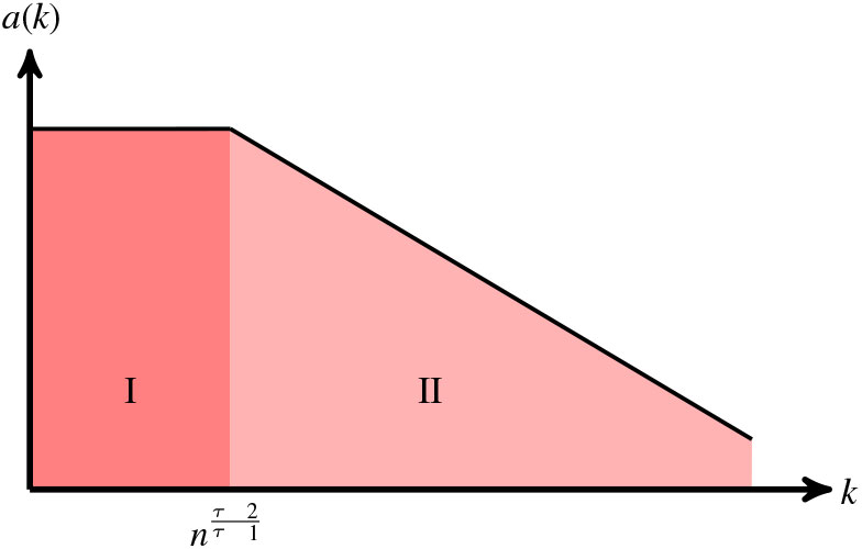
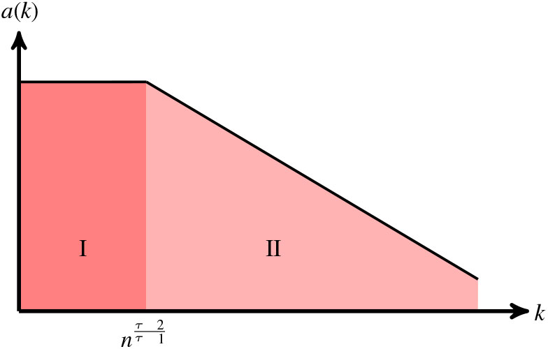
Figure 2 illustrates the behaviour of
 $a_{\varepsilon_n}(k,G_n)$
. First, it stays flat and does not depend on k. After that,
 $a(k,G_n)$
starts decreasing in k, which shows that the erased configuration model indeed is a disassortative random graph. Theorem 1 shows that
 $n^{(\tau-2)/(\tau-1)}$
serves as a threshold. Thus, the negative degree–degree correlations due to the single-edge constraint only affect vertices of degrees at least
 $n^{(\tau-2)/(\tau-1)}$
. This can be understood as follows. In the erased configuration model the maximum contribution to
 $a_{\varepsilon_n}(k,G)$
(see Propositions 1 and 2) comes from vertices with degrees proportional to
 $n/k$
. The maximal degree in an observation of n i.i.d. power-law distributed samples is proportional to
 $n^{1/(\tau-1)}$
w.h.p. Therefore, if
 $k\ll n^{(\tau-2)/(\tau-1)}$
, such vertices with degree proportional to
 $n/k$
do not exist w.h.p. This explains the two regimes.
Illustration of the behaviour of
 $a(k,G_n)$
in the erased configuration model.
For k small,
 $a_{\varepsilon_n}(k,G_n)$
converges to a stable random variable, as was also shown in [Reference Yao, van der Hoorn and Litvak45] for k fixed. Thus, for k small, different instances of the erased configuration model show wild fluctuations. The joint convergence in k of Remark 1 shows that
 $a(k,G_n)$
still forms a flat curve in k for one realization of an erased configuration model when k is small. In contrast,
 $a_{\varepsilon_n}(k,G_n)$
converges to a constant for large k-values, so that different realizations of erased configuration models result in similar
 $a_{\varepsilon_n}(k,G_n)$
-values.
2.2. Sketch of the proof
We now give a heuristic proof of Theorem 1. Conditionally on the degrees, the probability that vertices with degrees
 $D_i$
and
 $D_j$
are connected in the erased configuration model can be approximated by [Reference van der Hofstad, Hooghiemstra and Van Mieghem24]
 $1-{{\rm e}}^{-D_iD_j/\mu n}$
. Let
 $v\in M_{\varepsilon_n}(k)$
, and let
 $X_{iv}$
denote the indicator that vertex i is connected to v. The expected degree of a neighbour of v can then be approximated by
 \begin{equation}a_{\varepsilon_n}(k,G_n)\approx k^{-1}\sum_{i\in[n]}{D_i{{\mathbb{P}}({X_{iv}=1})}} \approx k^{-1}\sum_{i\in [n]}D_i(1-{{\rm e}}^{-D_ik/(\mu n)}).\end{equation}
The maximum degree in an i.i.d. sample from (3) scales as
 $n^{1/(\tau-1)}$
w.h.p. Thus, as long as
 $k\ll n^{(\tau-2)/(\tau-1)}$
, we can Taylor-expand the exponential so that
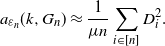 \begin{equation*}a_{\varepsilon_n} (k,G_n)\approx \frac{1}{\mu n}\sum_{i\in [n]}D_i^2.\end{equation*}
Because
 $ (D_i)_{i\in[n]}$
are samples from a power-law distribution with infinite second moment, the Stable Law Central Limit Theorem gives Theorem 1(i).
When
 $k\gg n^{(\tau-2)/(\tau-1)}$
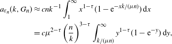
, we approximate the sum in (7) by the integral
 \begin{equation*}\begin{aligned}[b]a_{\varepsilon_n} (k,G_n)& \approx cnk^{-1}\int_{1}^{\infty}x^{1-\tau}(1-{{\rm e}}^{-xk/(\mu n)})\,{{\rm d}} x \\ & = c\mu^{2-\tau}\bigg(\frac{n}{k}\bigg)^{3-\tau}\int_{k/(\mu n)}^{\infty}y^{1-\tau}(1-{{\rm e}}^{-y})\,{{\rm d}} y,\end{aligned}
\end{equation*}
using the degree distribution (3) and the change of variables
 $y=xk/(\mu n)$
. When
 $ k \ll n$
, we can approximate this by
 \begin{equation*} a_{\varepsilon_n} (k,G_n)\approx c\mu^{2-\tau}\bigg(\frac{n}{k}\bigg)^{3-\tau}\int_{0}^{\infty}y^{1-\tau}(1-{{\rm e}}^{-y})\,{{\rm d}} y=-c\mu^{2-\tau}\bigg(\frac{n}{k}\bigg)^{3-\tau}\Gamma(2-\tau).\end{equation*}
The proof of Theorem 1(ii) then consists of showing that the above approximations are indeed valid. We prove Theorem 1 in detail in Sections 3.2 and 3.3.
2.3. Rank-1 inhomogeneous random graphs
We now turn to the rank-1 inhomogeneous random graph (or hidden variable model). This model constructs simple graphs with soft constraints on the degree sequence [Reference Boguñá and Pastor-Satorras9, Reference Chung and Lu16]. The graph consists of n vertices with weights
 $ (h_i)_{i\in[n]}$
. These weights are an i.i.d. sample from the power-law distribution (3). We denote the average value of the weights by
 $\mu$
. Then, every pair of vertices with weights (h,h’) is connected with probability p(h,h’). In this paper, we take
 \begin{equation*}p(h,h')=\min({h h'}/(\mu n),1),\end{equation*}
which is the Chung–Lu version of the rank-1 inhomogeneous random graph [Reference Chung and Lu16]. This connection probability ensures that the degree of a vertex with weight h will be close to h [Reference Boguñá and Pastor-Satorras9]. We show the following result.
Theorem 2. (
 $a(k,G_n)$
in the rank-1 inhomogeneous random graph.) Let
 $ (G_n)_{n\geq 1}$
be a sequence of rank-1 inhomogeneous random graphs on n vertices, where the weights are an i.i.d. sample from (3). Take
 $\varepsilon_n = 1/(\log(\log(n)))$
and let
 $\Gamma$
denote the gamma function.
(i) For
$1\ll k\ll n^{(\tau-2)/(\tau-1)}/\log(n)$
,
where\begin{equation*}\frac{a_{\varepsilon_n}(k,G_n)}{n^{(3-\tau)/(\tau-1)}}{{\stackrel{d}{\longrightarrow}}} \frac{1}{\mu}\bigg(\frac{2c \Gamma(\frac{5}{2}-\frac{1}{2}\tau )}{ (\tau-1)(3-\tau)}\cos\bigg(\frac{\pi(\tau-1)}{4}\bigg)\bigg)^{2/(\tau-1)} \mathcal{S}_{(\tau-1)/2},\end{equation*}
$\mathcal{S}_{(\tau-1)/2}$
is a stable random variable.(ii) For
$n^{(\tau-2)/(\tau-1)}\ll k\ll n^{1/(\tau-1)}/\log(n)$
,
(8)\begin{equation}\frac{a_{\varepsilon_n}(k,G_n)}{n^{3-\tau}k^{\tau-3}}{{\stackrel{{\mathbb{P}}}{\longrightarrow}}} \frac{c \mu^{2-\tau}}{(3-\tau)(\tau-2)}.\end{equation}




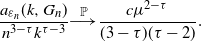
Theorem 2 is almost identical to Theorem 1. The proof of Theorem 2 exploits the deep connection between the two models, and essentially carries over the results for the erased configuration model to the rank-1 inhomogeneous random graph. The similarity can be understood by noticing that in the erased configuration model the probability that vertices i and j with degrees
 $D_i$
and
 $D_j$
are connected can be approximated by
 $1-\exp(-D_iD_j/L_n)$
which is close to
 $$\min\bigg(1,\frac{D_iD_j}{\mu n}\bigg),$$
the connection probability in the rank-1 inhomogeneous random graph. Arguments similar to those that led to (7) show that
 $a_{\varepsilon_n}(k,G_n)$
can be approximated by
 \begin{equation*}a_{\varepsilon_n}(k,G_n)\approx k^{-1}\sum_{i\in[n]}h_i\min(h_ik/\mu n,1).\end{equation*}
This sum behaves very similarly to the sum in (7), so that the only difference between Theorem 1 and 2 is the limiting constants in (6) and (8). The main difference between the two models is that in the rank-1 inhomogeneous random graph the presence of all edges is independent as soon as the weights are sampled. This is not true in the erased configuration model, because we know that a vertex with sampled degree
 $D_i$
cannot have more than
 $D_i$
neighbours, creating dependence between the presence of edges incident to vertex i. We show that these correlations between the presence of different edges in the erased configuration model are small enough for
 $a_{\varepsilon_n}(k,G_n)$
to behave similarly in the erased configuration model and the rank-1 inhomogeneous random graph.
2.4. Hyperbolic random graphs
The third random graph model we consider is the hyperbolic random graph. This model was introduced in [Reference Krioukov, Papadopoulos, Kitsak, Vahdat and Boguná31] and samples n vertices on a disk of radius
 $R=2\log(n/\nu)$
, where the density of the radial coordinate r a vertex
 $p=(r,\phi)$
is
 \begin{equation*}\rho(r)=\alpha\frac{\sinh(\alpha r)}{\cosh(\alpha R)-1}\end{equation*}
with
 $\alpha=(\tau-1)/2$
. The angle of p is sampled uniformly from
 $[0,2\pi]$
. Then, two vertices are connected if their hyperbolic distance is at most R. The hyperbolic distance of points
 $u=(r_u,\phi_u)$
and
 $v=(r_v,\phi_v)$
is defined by
 \begin{equation}\cosh({{\rm d}} (u,v))=\cosh(r_u)\cosh(r_v)-\sinh(r_u)\sinh(r_v)\cos(\theta_{uv}),\end{equation}
where
 $\theta_{uv}$
denotes the relative angle between
 $\phi_u$
and
 $\phi_v$
. This creates a simple random graph with power-law degrees with exponent
 $\tau$
[Reference Krioukov, Papadopoulos, Kitsak, Vahdat and Boguná31]. The parameter
 $\nu$
fixes the average degree of the graph.
The hyperbolic random graph creates simple sparse random graphs with power-law degrees, but in contrast to the erased configuration model and the rank-1 inhomogeneous random graph, can at the same time create many triangles due to its geometric nature [Reference Candellero and Fountoulakis14, Reference Krioukov, Papadopoulos, Kitsak, Vahdat and Boguná31]. In both the rank-1 inhomogeneous random graph and the erased configuration model, the connection probabilities of different pairs of vertices are (almost) independent. In the hyperbolic random graph, this is not true. When u is connected to v and u is connected to w, then v and w should also be close to one another by the triangle inequality. However, if we define the type of a vertex as
 \begin{equation*}t(u)={{\rm e}}^{(R-r_u)/2} {,}\end{equation*}
then we show that we can approximate the probability that vertices u and v are connected by
 \begin{equation*}{{\mathbb{P}}({X_{uv}=1\mid t(u),t(v)})}=\begin{cases} \frac{2}{\pi}\sin^{-1}(\nu t(u)t(v)/n) & \nu t(u)t(v)/n \lt 1,\\1 & \nu t(u)t(v)/n\geq 1,\end{cases}\end{equation*}
which behaves similarly to the connection probability in the rank-1 inhomogeneous random graph. Furthermore, by [Reference Bode, Fountoulakis and Müller7, Lemma 1.3], the density of
 $2\ln(t(u))$
can be written as
 \begin{equation*}f_{2\ln(t(u))}(x)=\bigg(\frac{\tau-1}{2}\bigg)\,{{\rm e}}^{-(\tau-1)x/2}(1+{\mathrm{o}}(1)),\end{equation*}
where the
 ${\mathrm{o}}(1)$
term is with respect to the network size n. Therefore,
 \begin{equation}{{\mathbb{P}}({t(u)>x})}={{\mathbb{P}}({2\ln(t(u))>2\ln(x)})}=x^{-\tau+1}(1+{\mathrm{o}}(1)),\end{equation}
so that on a high level the hyperbolic random graph can be interpreted as a rank-1 inhomogeneous random graph with
 $ (t(u))_{u\in[n]}$
as weights (see [Reference Bode, Fountoulakis and Müller7, Section 1.1.1] for a more elaborate discussion).
The next theorem shows that indeed the behaviour of
 $a_{\varepsilon_n}(k,G_n)$
in the hyperbolic random graph is similar to the rank-1 inhomogeneous random graph.
Theorem 3. (
 $a(k,G_n)$
in the hyperbolic random graph.) Let
 $ (G_n)_{n\geq 1}$
be a sequence of hyperbolic random graphs on n vertices with power-law degrees with exponent
 $\tau$
and parameter
 $\nu$
. Take
 $\varepsilon_n = 1/\log(\log(n))$
and let
 $\Gamma$
denote the gamma function.
(i) For
$1\ll k\ll n^{(\tau-2)/(\tau-1)}/\log(n)$
,
where\begin{equation*}\frac{a_{\varepsilon_n}(k,G_n)}{n^{(3-\tau)/(\tau-1)}}{{\stackrel{d}{\longrightarrow}}}\frac{2\nu}{\pi}\bigg(\frac{2}{3-\tau}\Gamma\bigg(\frac{5}{2}-\frac{1}{2}\tau \bigg)\cos\bigg(\frac{\pi(\tau-1)}{4}\bigg)\bigg)^{2/(\tau-1)}\mathcal{S}_{(\tau-1)/2},\end{equation*}
$\mathcal{S}_{(\tau-1)/2}$
is a stable random variable.(ii) For
$ n^{(\tau-2)/(\tau-1)}\ll k \ll n^{1/(\tau-1)}/\log(n)$
,
\begin{equation*}\frac{a_{\varepsilon_n}(k,G_n)}{n^{3-\tau}k^{\tau-3}}{{\stackrel{{\mathbb{P}}}{\longrightarrow}}}\frac{(\tau-1) \nu\sqrt{\pi}\Gamma(\frac32-\frac{\tau}{2})}{2(\tau-2)\Gamma(2-\frac{\tau}{2})}\bigg(\frac{2(\tau-1)}{\pi(\tau-2)}\bigg)^{3-\tau}.\end{equation*}





2.5. Discussion
2.5.1. Universality
The behaviour of
 $a_{\varepsilon_n}(k,G_n)$
is universal across the three null models we consider. The erased configuration model and the rank-1 inhomogeneous random graph are closely related. They are known to behave similarly, for example, under critical percolation [Reference Bhamidi, Dhara, van der Hofstad and Sen4, Reference Bhamidi, Sen and Wang6], in terms of distances [Reference van den Esker, van der Hofstad and Hooghiemstra18] when
 $\tau>3$
, and in terms of clustering when
 $\tau\in(2,3)$
[Reference Stegehuis, van der Hofstad, van Leeuwaarden and Janssen41]. The hyperbolic random graph typically shows different behaviour, for example in terms of clustering [Reference Candellero and Fountoulakis14, Reference Gugelmann, Panagiotou and Peter22], or connectivity [Reference Bode, Fountoulakis and Müller7, Reference Bode, Fountoulakis and Müller8]. Still, the behaviour of
 $a_{\varepsilon_n}(k,G_n)$
is similar in the hyperbolic random graph and the other two null models. In all three null models, the main contribution for
 $k\gg n^{(\tau-2)/(\tau-1)}$
comes from vertices with degrees proportional to
 $n/k$
(see Propositions 1 and 2). In the hyperbolic random graph, we can relate this maximum contribution to the geometry of the hyperbolic sphere. A vertex i of degree k has radius
 $r_i\approx R-2\log(k)$
. Similarly, a vertex j of degree
 $ n/(\nu k)$
has radius
 $r_j\approx R-2\log( n/(k\nu))=2\log(k)$
. Then,
 $r_j\approx R-r_i$
, so that the major contributing vertices have radial coordinate proportional to
 $R-r_i$
.
2.5.2. Expected average nearest-neighbour degree
In Theorems 1–3 we show that
 $a_{\varepsilon_n}(k,G_n)$
converges in probability to a stable random variable when k is small. Thus, when we generate many samples of random graphs, for fixed k, the distribution of the values of
 $a_{\varepsilon_n}(k,G_n)$
across the different samples will look like a stable random variable. We can also study the expected value of
 $a(k,G_n)$
across the different samples. For the erased configuration model for example, we can show that (see Section 3.4)
 \begin{equation}\lim_{n\to\infty}\frac{{{\mathbb{E}}[{a(k,G_n)}]}}{(n/k)^{3-\tau}}=-c\mu^{2-\tau}\Gamma(2-\tau).\end{equation}
The difference between the scaling of the expected value of
 $a(k,G_n)$
and the typical behaviour of
 $a(k,G_n)$
in Theorem 1(i) is caused by high-degree vertices. In typical degree sequences, the maximum degree is proportional to
 $n^{1/(\tau-1)}$
. It is unlikely that vertices with higher degrees are present, but if they are, they have a high impact on the average nearest-neighbour degree of low-degree vertices, causing the difference between the expected average nearest-neighbour degree and the typical average nearest-neighbour degree. Thus, the expected value of
 $a(k,G_n)$
is not very informative when k is small, since Theorem 1 shows that
 $a(k,G_n)$
will almost always be smaller than its expected value when k is small.
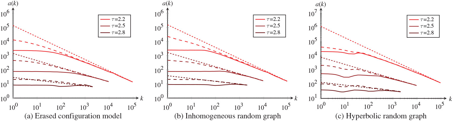
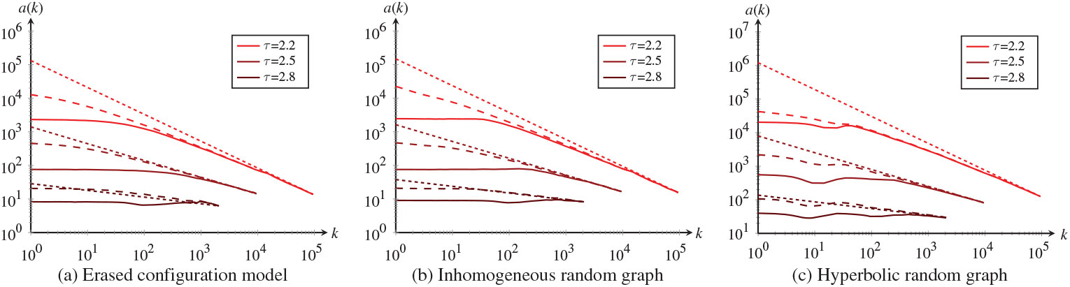
Figure 3 illustrates this difference in terms of the mean and median value of
 $a(k,G_n)$
over many realizations of the erased configuration model, the rank-1 inhomogeneous random graph, and the hyperbolic random graph. Here indeed we see that the expected average neighbour degree scales as a power of k over the entire range of k, where the median shows the straight part of the curve from Theorem 1. Thus, it is important to distinguish between mean and median of
 $a(k,G_n)$
when simulating random graphs.
 $a(k,G_n)$
for different random graph models with
 $n=10^6$
. The solid line is the median of
 $a(k,G_n)$
over
 $10^4$
realizations of the random graph, and the dashed line is the average over these realizations. The dotted line is the asymptotic slope
 $k^{\tau-3}$
.
2.5.3. Vertices of degree k
Definition (1) assumes that a vertex of degree k is present. For large values of k, this is a rare event, by (3). Indeed, vertices of degree at most
 $n^{1/\tau}$
are present with high probability in the erased configuration model, whereas the probability that a vertex of degree
 $k\gg n^{1/\tau}$
is present tends to zero in the large network limit [Reference Yao, van der Hoorn and Litvak45]. We avoid this problem by averaging
 $a(k,G_n)$
over a small range of degrees. Another option is to condition on the event that a vertex of degree k is present. Our proofs for
 $k\ll n^{(\tau-2)/(\tau-1)}$
for the erased configuration model can easily be adjusted to condition on this event. For k larger, we leave the behaviour of
 $a(k,G_n)$
conditionally on a vertex of degree k being present open for further research.
2.5.4. Fixed degrees
In the proof of Theorem 1 we show that the fluctuations that come with the stable laws for small k are not present when we condition on the degree sequence. Thus, the large fluctuations in
 $a_{\varepsilon_n}(k,G_n)$
for small k are caused by fluctuations of the i.i.d. degrees, weights, or radii. For a given real-world network, its degrees are often preserved, and many erased configuration models or inhomogeneous random graphs with the same observed degree sequence are created. In this fixed-degree setting, the sample-to-sample fluctuations of
 $a_{\varepsilon_n}(k,G_n)$
are relatively small.
2.5.5 Relation with local clustering
The local clustering coefficient c(k) of vertices of degree k measures the probability that two randomly chosen neighbours af a randomly chosen vertex of degree k are connected. In many real-world networks as well as simple null models, c(k) decreases as a function of k [Reference Boguñá and Pastor-Satorras9, Reference van der Hofstad, Janssen, van Leeuwaarden and Stegehuis26, Reference Ravasz and Barabási39, Reference Stegehuis, van der Hofstad, van Leeuwaarden and Janssen41, Reference Vázquez, Pastor-Satorras and Vespignani43]. The relation between the decay rate of c(k) and the decay rate of a(k) has been investigated for the rank-1 inhomogeneous random graph, where it was shown that
 $c(k) \lt a(k)/k$
[Reference Serrano and Boguñá40]. Using recent results for c(k) on the erased configuration model and the rank-1 inhomogeneous random graph, we can make the relation between c(k) and a(k) more precise. When
 $k\gg\sqrt{n}$
, c(k) in the erased configuration model satisfies [Reference van der Hofstad, Janssen, van Leeuwaarden and Stegehuis26]
 \begin{equation*}c(k)=c^2\Gamma(2-\tau)^2\mu^{3-2\tau}n^{5-2\tau}k^{2\tau-6}(1+{{\mathrm{o}}_{\scriptscriptstyle{\mathbb{P}}}}(1)).\end{equation*}
Then, by Theorem 1, when
 $k\gg \sqrt{n}$
,
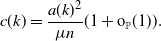 \begin{equation}c(k)=\frac{a(k)^2}{\mu n}(1+{{\mathrm{o}}_{\scriptscriptstyle{\mathbb{P}}}}(1)).\end{equation}
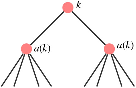
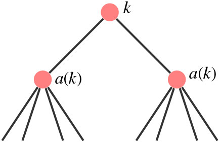
Intuitively, we can see this relationship in the following way. Pick two neighbours of a vertex of degree k. By definition, these vertices have degree a(k) on average. See Figure 4. Since
 $k\gg\sqrt{n}$
, by Theorem 2,
 $a(k)\ll\sqrt{n}$
. Therefore, the probability of two vertices with weight a(k) being connected is approximately
 $1-{{\rm e}}^{-a(k)^2/\mu n}\approx a(k)^2/\mu n$
. Since the clustering coefficient can be interpreted as the probability that two randomly chosen neighbours are connected, the clustering coefficient should satisfy
 $c(k)\sim a(k)^2/\mu n$
when
 $k\gg \sqrt{n}$
. In particular, the decay of the clustering coefficient should be twice as fast as the decay of the average neighbour degree. Analytical results on c(k) on the rank-1 inhomogeneous random graph show that (12) is also the correct relation between clustering and degree correlations in the rank-1 inhomogeneous random graph [Reference Stegehuis, van der Hofstad, van Leeuwaarden and Janssen41]. Future research might explore the relation between c(k) and a(k) in other null models, such as the hyperbolic random graph or the preferential attachment model. It would also be interesting to see if the difference between expectation and typical behaviour that is present in a(k) also occurs for the local clustering coefficient c(k).
The neighbours of a vertex of degree k have average degree a(k).
2.5.6 Correlations in the hyperbolic random graph
The relation in (12) is based on the fact that in the erased configuration model and the rank-1 inhomogeneous random graph the connection probabilities of pairs of vertices (i, j), (i, k), and (j, k) are (almost) independent. In the hyperbolic random graph, the geometry causes a strong dependence between these connection probabilities. If vertices j and k are neighbours of i, they are likely to be geometrically close to one another due to the triangle inequality. This makes the probability that j and k are connected larger than in the rank-1 inhomogeneous random graph or the erased configuration model. These correlations do not play a role when computing
 $a(k,G_n)$
, since it only involves the connection probability of two different vertices. When computing statistics of the hyperbolic random graph that include three-point correlations, the equivalence between the hyperbolic random graph and the rank-1 inhomogeneous random graph may fail to hold, as in the example of c(k).
Interestingly, the number of cliques was also shown to be similar in the hyperbolic random graph, the rank-1 inhomogeneous random graph and the erased configuration model [Reference Friedrich and Krohmer20], even though cliques clearly involve three-point correlations. Cliques in the hyperbolic random graph are typically formed between vertices at radius proportional to
 $R/2$
[Reference Friedrich and Krohmer20], so that their degrees are proportional to
 $\sqrt{n}$
[Reference Bode, Fountoulakis and Müller7]. These vertices form a dense core, which is very similar to what happens in the erased configuration model and the rank-1 inhomogeneous random graph [Reference Janson and Luczak29]. In the erased configuration model, many other small subgraphs typically occur between vertices of degrees proportional to
 $\sqrt{n}$
[Reference van der Hofstad, van Leeuwaarden and Stegehuis27]. It would be interesting to see if the number of these small subgraphs behaves similarly in the hyperbolic random graph.
3. Average nearest-neighbour degree in the ECM
In this section, we prove Theorem 1. For
 $k\ll n^{{(\tau-2)}/{(\tau-1)}}/\log(n)$
, we couple the degrees of neighbours of a uniformly chosen vertex of degree k to i.i.d. samples of the size-biased degree distribution in Section 3.2. When
 $k\gg n^{{(\tau-2)}/{(\tau-1)}}$
, this coupling is no longer valid. We then show in Section 3.3 that a specific range of degrees contributes most to
 $a_{\varepsilon_n}(k,G_n)$
.
3.1. Preliminaries
We say that
 $X_n={{\mathrm{O}}_{\scriptscriptstyle{\mathbb{P}}}({b_n})}$
for a sequence of random variables
 $ (X_n)_{n\geq 1}$
if
 $|X_n|/b_n$
is a tight sequence of random variables, and
 $X_n={{\mathrm{o}}_{\scriptscriptstyle{\mathbb{P}}}}(b_n)$
if
 $X_n/b_n{{\stackrel{{\mathbb{P}}}{\longrightarrow}}} 0$
. Let
 $L_n$
denote the total number of half-edges, so that
 $L_n=\sum_i D_i$
. We define the events
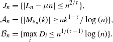 \begin{align} J_n& =\{{|{L_n-\mu n}|}\leq n^{2/\tau}\}, \notag \\ \mathcal{A}_n& =\{|M_{\varepsilon_n}(k)|\geq n k^{1-\tau}/\log(n)\}{,}\nonumber\\ \mathcal{B}_n& =\{\max_iD_i\leq n^{1/(\tau-1)}\log(n)\} {.}\end{align}
By [Reference van der Hofstad, van der Hoorn, Litvak and Stegehuis25, Lemma 2.3],
 ${{\mathbb{P}}({J_n})}\to 1$
as
 $n\to\infty$
. Furthermore, since the degree sequence is an i.i.d. sample from (3), also
 ${{\mathbb{P}}({\mathcal{B}_n})}\to 1$
. Note that
 $\mathcal{A}_n$
implies that
 $|M_{\varepsilon_n}(k)|\geq 1$
as long as
 $k\ll n^{1/(\tau-1)}/\log(n)$
. Below, we will show that
 ${{\mathbb{P}}({\mathcal{A}_n})}\to 1$
for
 $k\ll n^{1/(\tau-1)}/\log(n)$
. Throughout the rest of the paper, we will often condition on the event
 \begin{equation}\Lambda_n = J_n\cap \mathcal{A}_n\cap\mathcal{B}_n.\end{equation}
Note that
 ${{\mathbb{P}}({\Lambda_n})}\to 1$
.
In the rest of this paper, we will often condition on the degree sequence. For some event
 $\mathcal{E}$
, we use the notation
 ${{\mathbb{P}}_n({\mathcal{E}})}={{\mathbb{P}}({\mathcal{E}\mid (D_i)_{i\in[n]}})}$
, and we define
 ${\mathbb{E}}_n$
and
 $\text{Var}_n$
similarly, where we often assume that the event
 $\Lambda_n$
holds. In this notation
 ${{\mathbb{P}}_n({\mathcal{E}_1\mid\mathcal{E}_2})}={{\mathbb{P}}({\mathcal{E}_1\mid \mathcal{E}_2,(D_i)_{i\in[n]}})}$
. In this notation, we often work on the event
 $\Lambda_n$
. That is, we assume that the degree sequence satisfies the event
 $\Lambda_n$
, and we compute
 ${{\mathbb{P}}({\mathcal{E}\mid (D_i)_{i\in[n]}\in\Lambda_n})}$
.
We often want to interchange the sampled degree of a vertex i,
 $D_i$
and its resulting degree
 ${D^{\scriptscriptstyle\mathrm{(er)}}}_i$
. The next lemma shows that
 $D_i$
and
 ${D^{\scriptscriptstyle\mathrm{(er)}}}_i$
are close.
Leema 1. Let G be an erased configuration model where the degrees are i.i.d. samples from a power-law distribution with
 $\tau\in(2,3)$
. Assume the event
 $J_n\cap \mathcal{B}_n\cap\mathcal{D}_n(D_i)$
, where
 \begin{equation*} \mathcal{D}_n(D_i)=\bigg\{ \sum_{j \in[n]}\psi\bigg(\frac{D_iD_j}{\mu n}\bigg)\leq D_i^{\tau-1}n^{1-\tau}\log(n)\bigg\},
\end{equation*}
and
 $\psi(x)=x-1+{{\rm e}}^{-x}$
. Then,
 \begin{equation}{{\mathbb{P}}_n({D_i-{D^{\scriptscriptstyle\mathrm{(er)}}}_i>\varepsilon D_i})}\leq {{\mathrm{O}}({\varepsilon^{-1}({D_i}/{n})^{\tau-2}\log(n)})}+{{\mathrm{O}}({\varepsilon^{-1}{D_i}/{n}})}.\end{equation}
Note that by [Reference van der Hoorn and Litvak28, Theorem 3(ii)], for D distributed as in (3),
 ${{\mathbb{E}}[{\psi(D/t)}]}={\mathrm{O}}(t^{-(\tau-1)})$
so that
 \begin{equation*}{{\mathbb{E}}[{\psi(D_iD_j/(\mu n))\mid D_i}]}={\mathrm{O}}(D_i^{\tau-1}n^{1-\tau}).\end{equation*}
This shows that for all
 $D_i$
,
 ${{\mathbb{P}}({\mathcal{D}_n(D_i)})}\to 1$
.
Proof. We use [Reference van der Hofstad, Hooghiemstra and Van Mieghem24, (4.9)], which calculates p(n, m, L), the probability that a set of n half-edges does not connect to another set of m half-edges, when the total number of half-edges equals L. Then, choosing
 $n=D_i, m=D_j$
yields
 $p(D_i,D_j,L_n)={{\mathbb{P}}_n({X_{ij}=0})}$
, so that by [Reference van der Hofstad, Hooghiemstra and Van Mieghem24, (4.9)]
 \begin{equation*}{{\mathbb{P}}_n({X_{ij}=0})}\leq \prod_{s=0}^{D_i-1}\bigg(1-\frac{D_i}{L_n-2D_i-1}\bigg)+\frac{D_i^2D_j}{(L_n-2D_i)^2}\leq {{\rm e}}^{-D_iD_j/L_n}+\frac{D_i^2D_j}{(L_n-2D_i)^2}{.}\end{equation*}
Let
 $\psi(x)=x-1+{{\rm e}}^{-x}$
. The expected number of erased edges at vertex i satisfies
 \begin{align*}{{\mathbb{E}}_n[{D_i-{D^{\scriptscriptstyle\mathrm{(er)}}}_i}]} & =D_i-\sum_{j\in[n]}(1-{{\mathbb{P}}_n({X_{ij}=0})}) \notag\\ &\leq \sum_{j\in[n]}\bigg(\frac{D_iD_j}{L_n}-1+ {{\rm e}}^{-D_iD_j/L_n}+\frac{D_i^2D_j}{(L_n-2D_i)^2}\bigg) \notag \\ & =\sum_{j\in [n]}\psi\bigg(\frac{D_iD_j}{L_n}\bigg)+{\mathrm{O}}\bigg(\frac{D_i^2}{L_n}\bigg) \notag \\ & = \sum_{j\in [n]}\psi\bigg(\frac{D_iD_j}{\mu n}\bigg)(1+{\mathrm{o}}(1))+{{\mathrm{O}}\bigg({\frac{D_i^2}{n}}\bigg)} {.}\end{align*}
Thus, on the event
 $\mathcal{D}_n$
,
 \begin{equation}{{\mathbb{E}}_n [{D_i-{D^{\scriptscriptstyle\mathrm{(er)}}}_i}]}= {{\mathrm{O}}({n^{-\tau+2}D_i^{\tau-1}\log(n)})}+{{\mathrm{O}}({{D_i^2}/{n}})}.\end{equation}
Using the Markov inequality, we obtain
 \begin{equation*}{{\mathbb{P}}_n({D_i-{D^{\scriptscriptstyle\mathrm{(er)}}}_i>\varepsilon D_i})}\leq {{\mathrm{O}}({\varepsilon^{-1}({D_i}/{n})^{\tau-2}\log(n)})}+{{\mathrm{O}}({\varepsilon^{-1}{D_i}/{n}})}.\end{equation*}
We now use Lemma 1 to show that
 ${{\mathbb{P}}({\mathcal{A}_n})}\to 1$
, with
 $\mathcal{A}_n$
as in (13). Let v be a uniformly chosen vertex and denote
 $I(k,\varepsilon_n)=[k(1-\varepsilon_n),k(1+\varepsilon_n)]$
. Then,
 \begin{align}{{\mathbb{E}} [{|M_{\varepsilon_n}(k)|}]}& =n{{\mathbb{P}}({{D^{\scriptscriptstyle\mathrm{(er)}}}_v \in I(k,\varepsilon_n)})}\nonumber\\& \geq n{{\mathbb{P}}({D_v \in I(k,\varepsilon_n/2)})}{{\mathbb{P}}({{D^{\scriptscriptstyle\mathrm{(er)}}}_v\in I(k,\varepsilon_n) \mid D_v\in I(k,\varepsilon_n/2)})}\nonumber\\
& \geq n{{\mathbb{P}}({D_v \in I(k,\varepsilon_n/2)})}{{\mathbb{P}}({D_v-{D^{\scriptscriptstyle\mathrm{(er)}}}_v\leq k\varepsilon_n/2 \mid D_v = k(1-\varepsilon_n/2), J_n,\mathcal{D}_n(k)})}\nonumber\\& \quad\,
\times {{\mathbb{P}}({J_n\cap \mathcal{D}_n(k)})}{.}\end{align}
Furthermore, for some
 $\tilde{C}_1>0$
,
 \begin{equation*}
{{\mathbb{P}}({D_v \in I(k,\varepsilon_n/2)})} = \sum_{i=k(1-\varepsilon_n)}^{k(1+\varepsilon_n)}i^{-\tau}\geq \tilde{C}_1\int_{k(1-\varepsilon_n)}^{k(1+\varepsilon_n)}x^{-\tau}\,{{\rm d}} x.
\end{equation*}
Therefore, using (17), for some
 $\tilde{C}_2>0$
,
 \begin{align*}
{{\mathbb{E}} [{|M_{\varepsilon_n}(k)|}]}& \geq \tilde{C}_1 n\int_{k(1-\varepsilon_n/2)}^{k(1+\varepsilon_n/2)}x^{-\tau}\,{{\rm d}} x(1-{\mathrm{O}}(\varepsilon_n^{-1}(k/n)^{\tau-2}\log(n))) \nonumber\\& =\tilde{C}_2nk^{1-\tau}\varepsilon_n(1+{\mathrm{o}}(1)),
\end{align*}
where we used (15) combined with the choice of
 $\varepsilon_n$
in Theorem 1. Thus,
 ${{\mathbb{P}}({\mathcal{A}_n})}\to 1$
for
 $k\ll n^{1/(\tau-1)}/\log(n)$
by the choice of
 $\varepsilon_n$
in Theorem 1.
3.2. Small k: coupling to i.i.d. random variables
In this section we investigate the behaviour of
 $a_{\varepsilon_n}(k,G_n)$
when
 $k\ll n^{(\tau-2)/(\tau-1)}/\log(n)$
. We first pick a random vertex
 $v\in M_{\varepsilon_n}(k)$
. We couple the degrees of the neighbours of v to i.i.d. copies of the size-biased degree distribution
 $D_n^*$
, where
 \begin{equation*}
{{\mathbb{P}}_n({D_n^*=j})}=\frac{j}{L_n}\sum_{i\in[n]}{{\bf 1}_{\{{D_i=j}\}}}.
\end{equation*}
We then use this coupling to compute
 $a_{\varepsilon_n} (k,G_n)$
.
Proof of Theorem 1(i). We first condition on the degree sequence
 $ (D_i)_{i\in[n]}\in \Lambda_n$
of (14), since
 ${{\mathbb{P}}({\Lambda_n})}\to 1$
. Let v be a vertex of degree d. In the configuration model, neighbours of v are constructed by pairing the half-edges of v uniformly to other half-edges. The distribution of the degree of a vertex attached to a uniformly chosen half-edge is given by
 $D_n^*$
. However, the degrees of the neighbours of v in the erased configuration model are not an i.i.d. sample of
 $D_n^*$
due to the fact that the half-edges should attach to distinct vertices that are different from v. We now couple the degrees of the neighbours of v by an i.i.d. sample of
 $D_n^*$
. Denote degrees of neighbours of v by
 $B_1,\ldots, B_{d}$
. Let
 $Y_1,\ldots, Y_d$
be i.i.d. samples of
 $D_n^*$
. We use a similar coupling as in [Reference Bhamidi, van der Hofstad and Hooghiemstra5, Construction 4.2] to couple
 $B_i$
to
 $Y_i$
. Set
 $V_0=v$
. Then, for
 $i\in[d]$
the coupling is defined in the following way.
Take a uniformly chosen half-edge (with replacement), let
$v_i'$
be the vertex attached to it, and set
$Y_i=D_{v'_i}$
.Sample a uniformly chosen half-edge from the set of half-edges not incident to
$ V_{i-1}$
. Let
$w_i$
denote the vertex incident to the chosen half-edge.If
$v'_i\notin V_{i-1}$
, then set
$B_i=Y_i$
. and
$V_i=V_{i-1}\cup v_i'$
.If
$v'_i \in V_{i-1}$
, set
$B_i=D_{w_i}$
and
$V_i=V_{i-1}\cup w_i$
.


Summarizing,
 \begin{equation*}
(Y_i,B_i)=\begin{cases}
(D_{v'_i},D_{v'_i}) & \text{when }v'_i\notin V_{i-1},\\
(D_{v'_i},D_{w_i}) & \text{when }v'_i \in V_{i-1},
\end{cases}
\end{equation*}
where
 $ (v'_i)_{i\in[d]}$
are vertices attached to uniformly chosen half-edges (with replacement), and
 $w_i$
are vertices attached to uniformly chosen half-edges from the set of half-edges not incident to
 $V_{i-1}$
.
Informally, at every step i we sample a uniformly chosen half-edge from all half-edges, and select the vertex
 $v'_i$
incident to it. If this vertex is different from all previously selected vertices and unequal to v, we declare the vertex to be a neighbour of v, and
 $B_i=Y_i=D_{v'_i}$
. If not, we redraw the selected half-edge to ensure that all neighbours of v are distinct and unequal to v, and declare the vertex attached to this half-edge,
 $w_i$
to be a neighbour of v and set
 $B_i=D_{w_i}$
.
When
 $B_s\neq Y_s$
,
 $B_s$
is drawn in a size-biased manner from the vertices that are not chosen yet. Then, because
 $D_i\geq 0$
for all i,
 \begin{equation*}
\begin{aligned}[b]
{{\mathbb{E}}_n [{B_s\mid V_s,B_s\neq Y_s}]} & =\frac{\sum_{i\notin V_s}D_i^2}{\sum_{i\notin V_s}D_i}\\
& \leq \frac{\sum_{i\in[n]}D_i^2}{\sum_{i\in [n]}D_i-\sum_{i\in V_s}D_i}\\
& =\frac{\sum_{i\in [n]} D_i^2}{\sum_{i\in [n]}D_i}\bigg(1+\frac{\sum_{i\in V_s}D_i}{\sum_{i\in [n]}D_i-\sum_{i\in V_s}D_i}\bigg).
\end{aligned}
\end{equation*}
On the event
 $\mathcal{B}_n$
,
 $D_{\max}\leq n^{1/(\tau-1)}\log(n)$
, so that
 $\sum_{i\in V_s}D_i\leq sD_{\max}={{\mathrm{O}}({sn^{1/(\tau-1)}\log(n)})}$
for all possible
 $V_s$
, so that for
 $s={\mathrm{o}}( n^{(\tau-2)/(\tau-1)}/\log(n))$
 \begin{equation}
{{\mathbb{E}}_n [{B_s\mid B_s\neq Y_s }]}=\frac{\sum_{i\in [n]} D_i^2}{L_n}(1+{\mathrm{o}}(1))={{\mathbb{E}} [{D_n^*}]}(1+{\mathrm{o}}(1)).
\end{equation}
Let
 $\mathcal{N}_{v}(U)$
denote a uniformly chosen neighbour of vertex v of degree
 ${\mathrm{o}}( n^{(\tau-2)/(\tau-1)}/\log(n))$
. Then, by (18) and the fact that
 ${{\mathbb{E}}_n [{Y_s}]}={{\mathbb{E}}_n [{D_n^*}]}$
,
 \begin{equation*}
{{\mathbb{E}}_n [{D_{\mathcal{N}_{v}(U)}}]} = {{\mathbb{E}} [{D_n^*}]}(1+{\mathrm{o}}(1)).
\end{equation*}
When
 $i\in M_{\varepsilon_n}(k)$
,
 ${D^{\scriptscriptstyle\mathrm{(er)}}}_i=k(1+{\mathrm{o}}(1))$
. Let
 $E_n$
denote the total number of erased edges in the erased configuration model. By [Reference van der Hoorn and Litvak28, Theorem 1],
 \begin{equation}
E_n={{\mathrm{O}}_{\scriptscriptstyle{\mathbb{P}}}({\min(n^{1/(\tau-1)},n^{4/(\tau-1)-2})})}.
\end{equation}
Then, conditionally on the degree sequence
 \begin{align*}
a_{\varepsilon_n}(k,G_n) & =\frac{1}{k |M_{\varepsilon_n}(k)|}\sum_{i \in M_{\varepsilon_n}(k)}\sum_{j\in\mathcal{N}_i}{D^{\scriptscriptstyle\mathrm{(er)}}}_j \notag \\& =\frac{1}{k |M_{\varepsilon_n}(k)|}\sum_{i \in M_{\varepsilon_n}(k)}\sum_{j\in\mathcal{N}_i}D_j-\frac{1}{k |M_{\varepsilon_n}(k)|}\sum_{i \in M_{\varepsilon_n}(k)}\sum_{j\in\mathcal{N}_i}(D_j-{D^{\scriptscriptstyle\mathrm{(er)}}}_j) \notag \\
& = (1+{\mathrm{o}}(1)){{\mathbb{E}}_n [{D_{\mathcal{N}_{V_k}(U)}}]} +{\mathrm{O}}(E_nk^{-1}|M_{\varepsilon_n}(k)^{-1}|) \notag \\&=(1+{\mathrm{o}}(1)){{\mathbb{E}}_n [{D_{\mathcal{N}_{V_k}(U)}}]} + {{\mathrm{O}}_{\scriptscriptstyle{\mathbb{P}}} ({k^{\tau-2}n^{-1}\log(n)\min(n^{{1}/{\tau-1}},n^{{4}/{\tau-1}-2})})},
\end{align*}
where
 $V_k$
denotes a uniformly chosen vertex in
 $M_{\varepsilon_n}(k)$
, and
 $\mathcal{N}_{V_k}(U)$
is a uniformly chosen neighbour of vertex
 $V_k$
. Here the third equality holds because the average nearest-neighbour degree averages over all neighbours of vertex j and over all vertices in
 $M_{\varepsilon_n}(k)$
, together with the fact that
 $D_{V_k}=k(1+{\mathrm{o}}(1))$
. The fourth equality follows from (19) and on the event
 $\mathcal{A}_n$
. Note that for
 $k\ll n^{(\tau-2)/(\tau-1)}/\log(n)$
and
 $\tau\in(2,3)$
, the last term is
 ${{\mathrm{o}}_{\scriptscriptstyle{\mathbb{P}}}}(1)$
. Then, conditionally on the degree sequence, on the event
 $\Lambda_n$
,
 \begin{equation}
a_{\varepsilon_n} (k,G_n) =(1+{\mathrm{o}}(1)){{\mathbb{E}}_n [{D_{\mathcal{N}_{V_k}(U)}}]}+{{\mathrm{o}}_{\scriptscriptstyle{\mathbb{P}}}}(1) =(1+{\mathrm{o}}(1))(\mu n)^{-1}\sum_{i\in [n]}D_i^2+{{\mathrm{o}}_{\scriptscriptstyle{\mathbb{P}}}}(1).
\end{equation}
For t large, we obtain from (3) that
 \begin{equation*}
{{\mathbb{P}}({D^2>t})}={{\mathbb{P}}({D>\sqrt{t}})}=\frac{c}{\tau-1}t^{(1-\tau)/2}(1+{\mathrm{o}}(1)).
\end{equation*}
We then use the Stable Law Central Limit Theorem (see e.g. [Reference Whitt44, Theorem 4.5.2]) to conclude that
 \begin{equation*}{\sum_{i\in [n]}D_i^2}/{\bigg(n^{2/(\tau-1)}\bigg(\frac{2c}{ (\tau-1)(3-\tau)} \Gamma\bigg(\frac{5}{2}-\frac{1}{2}\tau \bigg)\cos\bigg(\frac{\pi(\tau-1)}{4}\bigg)\bigg)^{2/(\tau-1)} \bigg)}{{\stackrel{d}{\longrightarrow}}} \mathcal{S}_{(\tau-1)/2},
\end{equation*}
where
 $\mathcal{S}_{(\tau-1)/2}$
is a stable random variable. Combining this with (20) results in
 \begin{equation*}
\frac{a_{\varepsilon_n} (k,G_n)}{n^{(3-\tau)/(\tau-1)}}{{\stackrel{d}{\longrightarrow}}} \frac{1}{\mu }\bigg(\frac{2c\Gamma(\frac{5}{2}-\frac{1}{2}\tau )}{ (\tau-1)(3-\tau)} \cos\bigg(\frac{\pi(\tau-1)}{4}\bigg)\bigg)^{2/(\tau-1)} \mathcal{S}_{(\tau-1)/2}.
\end{equation*}
To prove the joint convergence of Remark 1, note that, for fixed m, the probability that
 $M_{\varepsilon_n}(k_i)$
satisfies the condition in (13) for all
 $i\in[m]$
tends to 1, by a proof similar to the proof that
 $\mathcal{A}_n$
defined in (13) satisfies
 ${{\mathbb{P}}({\mathcal{A}_n})}\to 1$
. Thus, we may condition on the event that
 $M_{\varepsilon_n}(k_i)\geq nk^{1-\tau}/\log(n)$
for all
 $i\in[m]$
. Then, the fact that (20) is the same for all
 $k_i\ll n^{(\tau-2)/(\tau-1)}/\log(n)$
and it only depends on the degree sequence proves the joint convergence.
3.3. Large k
Now we study the value of
 $a_{\varepsilon_n}(k,G_n)$
when
 $k\gg n^{(\tau-2)/(\tau-1)}$
. We show that there exists a range of degrees
 $W_n^k(\delta)$
which gives the largest contribution to
 $a_{\varepsilon_n}(k,G_n)$
. For ease of notation, we write
 $a_{\varepsilon_n}(k)$
for
 $a_{\varepsilon_n}(k,G_n)$
in this section. We define
 \begin{equation}
W_n^k(\delta)= \{u\colon D_u\in [\delta \mu n/k,\mu n/(\delta k)]\},
\end{equation}
and we write
 \begin{equation}
\begin{aligned}[b]
a_{\varepsilon_n}(k) &= \frac{1}{k {|{M_{\varepsilon_n}(k)}|}}\sum_{i \in M_{\varepsilon_n}(k)}\sum_{j\in W_n^k(\delta)}{D^{\scriptscriptstyle\mathrm{(er)}}}_j+ \frac{1}{k {|{M_{\varepsilon_n}(k)}|}}\sum_{i \in M_{\varepsilon_n}(k)}\sum_{j\notin W_n^k(\delta)}{D^{\scriptscriptstyle\mathrm{(er)}}}_j\\
&=\!:\, a_{\varepsilon_n}(k,W_n^k(\delta))+a_{\varepsilon_n}(k,\bar{W}_n^k(\delta)),
\end{aligned}
\end{equation}
where
 $a_{\varepsilon_n}(k,W_n^k(\delta))$
gives the contribution to
 $a_{\varepsilon_n} (k)$
from vertices in
 $W_n^k(\delta)$
and
 $a_{\varepsilon_n}(k,\bar{W}_n(\varepsilon))$
denotes the contribution from vertices not in
 $W_n^k(\delta)$
. In the rest of this section, we prove the following two propositions, which together show that the largest contribution to
 $a_{\varepsilon_n}(k)$
indeed comes from vertices in
 $W_n^k(\delta)$
.
Proposition 1. (Minor contributions.) There exists
 $\kappa>0$
such that, for
 $k\ll n^{1/(\tau-1)}$
,
 \begin{equation*}
\limsup_{n\to\infty}\frac{{{\mathbb{E}} [{a_{\varepsilon_n}(k,\bar{W}_n^k(\delta))}]}}{(n/k)^{3-\tau}} ={{\mathrm{O}}({\delta^\kappa})}.
\end{equation*}
Proposition 2 (Major contributions.) For
 $ n^{(\tau-2)/(\tau-1)}\ll k \ll n^{1/(\tau-1)}/\log(n)$
,
 \begin{equation*}
\frac{a_{\varepsilon_n}(k,W_n^k(\delta))}{(n/k)^{3-\tau}}{{\stackrel{{\mathbb{P}}}{\longrightarrow}}} c\mu^{2-\tau}\int_{\delta}^{1/\delta}x^{1-\tau}(1-{{\rm e}}^{-x})\,{{\rm d}} x
\end{equation*}
We now show how these propositions prove part (ii) of Theorem 1.
Proof of Theorem 1(ii). By the Markov inequality and Proposition 1,
 \begin{equation*}
\frac{a_{\varepsilon_n}(k,\bar{W}_n^k(\delta))}{(n/k)^{3-\tau}}={{\mathrm{O}}_{\scriptscriptstyle{\mathbb{P}}}({\delta^\kappa})}.
\end{equation*}
Combining this with Proposition 2 results in
 \begin{equation}
\frac{a_{\varepsilon_n} (k)}{(n/k)^{3-\tau}}{{\stackrel{{\mathbb{P}}}{\longrightarrow}}} c\mu^{2-\tau}\int_{\delta}^{1/\delta}x^{1-\tau}(1-{{\rm e}}^{-x})\,{{\rm d}} x+{{\mathrm{O}}_{\scriptscriptstyle{\mathbb{P}}}({\delta^\kappa})}.
\end{equation}
Taking the limit of
 $\delta\to 0$
then proves the theorem.
The rest of this section is devoted to proving Propositions 1 and 2.
3.3.1. Conditional expectation
We first compute the expectation of
 $a_{\varepsilon_n}(k,W_n^k(\delta))$
conditionally on the degree sequence and on the event
 $ (D_i)_{i\in[n]}\in\Lambda_n\cap \mathcal{D}_n(\mu n/k)$
. Define the event
 \begin{equation*}
\mathcal{W}_n=\bigg\{\sum_{u\in W_n^k(\delta)}D_u-{D^{\scriptscriptstyle\mathrm{(er)}}}_u\leq | W_n^k(\delta)|nk^{1-\tau}\log(n)\bigg\}.
\end{equation*}
Using (16), we obtain
 \begin{equation*}
{\mathbb{E}}_n\Bigg[\sum_{u\in W_n^k(\delta)}{D^{\scriptscriptstyle\mathrm{(er)}}}_u-D_u\Bigg]=\sum_{u\in W_n^k(\delta)}{{\mathrm{O}}({D_u^{\tau-1}n^{2-\tau}})}=| W_n^k(\delta)|{{\mathrm{O}}({nk^{1-\tau}})},
\end{equation*}
so that
 ${{\mathbb{P}}({\mathcal{W}_n})}\to 1$
by the Markov inequality.
Leema 2. When
 $k\gg n^{(\tau-2)/(\tau-1)}$
, on the event
 $ (D_i)_{i\in[n]}\in \Lambda_n\cap\mathcal{W}_n\cap\mathcal{D}_n(\mu n/k)$
,
 \begin{equation*}
{{\mathbb{E}}_n [{a_{\varepsilon_n}(k,W_n^k(\delta))}]}=(1+{\mathrm{o}}(1))\frac{1}{k} \sum_{u\in W_n^k(\delta)}D_u(1-{{\rm e}}^{-D_uk/L_n}) .
\end{equation*}
Proof. Let
 $X_{ij}$
denote the indicator that i and j are connected. By (22),
 \begin{equation*}
{{\mathbb{E}}_n [{a_{\varepsilon_n}(k,W_n^k(\delta))}]}=\frac{1}{k{|{M_{\varepsilon_n}(k)}|}}\sum_{v\in M_{\varepsilon_n}(k)}\sum_{u\in W_n^k(\delta)}{D^{\scriptscriptstyle\mathrm{(er)}}}_u{{\mathbb{P}}_n({X_{uv}=1})}.
\end{equation*}
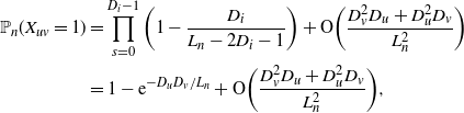
By [Reference van der Hofstad, Hooghiemstra and Van Mieghem24, (4.6) and (4.9)]
 \begin{align}
{{\mathbb{P}}_n({{X}_{uv}=1})}& =\prod_{s=0}^{D_i-1}\bigg(1-\frac{D_i}{L_n-2D_i-1}\bigg)+{{\mathrm{O}}\bigg({\frac{D_v^2D_u+D_u^2D_v}{L_n^2}}\bigg)}\nonumber\\& =1-{{\rm e}}^{-D_uD_v/L_n}+{{\mathrm{O}}\bigg({\frac{D_v^2D_u+D_u^2D_v}{L_n^2}}\bigg)},\end{align}
since
 $D_i,D_j={\mathrm{o}}(n)$
and
 $L_n=\mu n(1+{\mathrm{o}}(1))$
on
 $\Lambda_n$
. Thus, when
 $D_u\in \mu n/k[\delta,1/\delta]$
and
 $v\in M_{\varepsilon_n}(k)$
,
 \begin{equation*}
{{\mathbb{P}}_n({X_{uv}=1})}=(1-{{\rm e}}^{-D_uk/L_n})(1+{\mathrm{o}}(1)).
\end{equation*}
Since
 $\sum_{u\in W_n^k(\delta)}D_u=| W_n^k(\delta)|\Theta(n/k)$
and
 $n/k\gg nk^{1-\tau}\log(n)$
for
 $k\gg n^{(\tau-2)/(\tau-1)}$
, on the event
 $\mathcal{W}_n$
,
 \begin{align*}
\sum_{u\in W_n^k(\delta)}{D^{\scriptscriptstyle\mathrm{(er)}}}_u =\sum_{u\in W_n^k(\delta)}({D^{\scriptscriptstyle\mathrm{(er)}}}_u-D_u)+\sum_{u\in W_n^k(\delta)}D_u =(1+{\mathrm{o}}(1))\sum_{u\in W_n^k(\delta)}D_u
\end{align*}
Because
 $1-{{\rm e}}^{-D_uk/L_n}\in[1-{{\rm e}}^{-\delta},1-{{\rm e}}^\delta]$
when
 $u\in W_n^k(\delta)$
, this also shows that
 \begin{equation}
\sum_{u\in W_n^k(\delta)}{D^{\scriptscriptstyle\mathrm{(er)}}}_u(1-{{\rm e}}^{-D_uk/L_n})=(1+{\mathrm{o}}(1))\sum_{u\in W_n^k(\delta)}D_u(1-{{\rm e}}^{-D_uk/L_n}).
\end{equation}
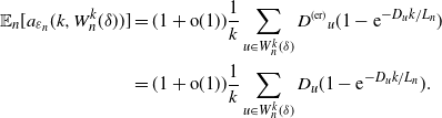
Thus, we obtain
 \begin{equation*}
\begin{aligned}[b]
{{\mathbb{E}}_n [{a_{\varepsilon_n}(k,W_n^k(\delta))}]} &=(1+{\mathrm{o}}(1))\frac{1}{k} \sum_{u\in W_n^k(\delta)}{D^{\scriptscriptstyle\mathrm{(er)}}}_u(1-{{\rm e}}^{-D_uk/L_n})\\
&=(1+{\mathrm{o}}(1))\frac{1}{k}\sum_{u\in W_n^k(\delta)}D_u(1-{{\rm e}}^{-D_uk/L_n}).
\end{aligned}
\end{equation*}
3.3.2. Convergence of conditional expectation
We shall now show that
 ${{\mathbb{E}}_n [{a_{\varepsilon_n}(k,W_n^k(\delta))}]}$
of Lemma 2 converges to a constant when we take the i.i.d. degrees into account.
Leema 3. When
 $k\gg n^{(\tau-2)/(\tau-1)}$
, on the event
 $ (D_i)_{i\in[n]}\in\Lambda_n\cap\mathcal{W}_n\cap\mathcal{D}_n(\mu n/k) $
,
 \begin{equation*}
\frac{{{\mathbb{E}}_n [{a_{\varepsilon_n}(k,W_n^k(\delta))}]}}{n^{3-\tau}k^{\tau-3}}{{\stackrel{{\mathbb{P}}}{\longrightarrow}}} c \mu^{2-\tau}\int_{\delta}^{1/\delta}x^{1-\tau}(1-{{\rm e}}^{-x})\,{{\rm d}} x.
\end{equation*}
Proof. First of all, notice that for
 $k\gg n^{(\tau-2)/(\tau-1)}$
 \begin{align*}
{{\mathbb{P}}({D\in[a,b]\mu n/k})}& =(1+{\mathrm{o}}(1))\sum_{t=\lceil a\mu n/k\rceil}^{\lfloor b \mu n/k\rfloor }ct^{-\tau}\leq (1+{\mathrm{o}}(1))\int_{a\mu n/k-1}^{b\mu n/k}cx^{-\tau}\,{{\rm d}} x\nonumber\\& =(1+{\mathrm{o}}(1))\frac{c}{\tau-1}\big((b\mu n/k)^{1-\tau}-(a\mu n/k-1)^{1-\tau}\big)\nonumber\\
& = (1+{\mathrm{o}}(1))\frac{c}{\tau-1}\big((b\mu n/k)^{1-\tau}-(a\mu n/k)^{1-\tau}\big)\nonumber\\& = (1+{\mathrm{o}}(1))\int_{a\mu n/k}^{b\mu n/k}cx^{-\tau}\,{{\rm d}} x.
\end{align*}
Similarly,
 \begin{align*}
{{\mathbb{P}}({D\in[a,b]\mu n/k})}& \geq (1+{\mathrm{o}}(1))\int_{\lceil a\mu n/k\rceil }^{\lfloor b\mu n/k\lfloor+1}cx^{-\tau}\,{{\rm d}} x \notag \\ & \geq (1+{\mathrm{o}}(1))\int_{a\mu n/k +1 }^{ b\mu n/k }cx^{-\tau}\,{{\rm d}} x \nonumber\\& = (1+{\mathrm{o}}(1))\int_{a\mu n/k}^{b\mu n/k}cx^{-\tau}\,{{\rm d}} x,
\end{align*}
so that
 \[
{{\mathbb{P}}({D\in[a,b]\mu n/k})} = (1+{\mathrm{o}}(1))\int_{a\mu n/k}^{b\mu n/k}cx^{-\tau}\,{{\rm d}} x\quad \text{when $k\gg n^{(\tau-2)/(\tau-1)}$.}
\]
Define the random measure
 \begin{equation}
{M^{\scriptscriptstyle(n)}}[a,b]=\frac{1}{\mu^{1-\tau}n^{2-\tau}k^{\tau-1}}\sum_{u\in[n]}{{\bf 1}_{\{{D_u\in[a,b]\mu n/k}\}}}.
\end{equation}
Since the degrees are i.i.d. samples from (3), the number of vertices with degrees in interval [a,b] is binomially distributed. Then,
 \begin{align*}
{M^{\scriptscriptstyle(n)}}[a,b] & = \frac{1}{\mu^{1-\tau}n^{2-\tau}k^{\tau-1}}{|{\{u\colon D_u\in[a,b]\mu n/k \}} |} \notag \\ & =(1+{{\mathrm{o}}_{\scriptscriptstyle{\mathbb{P}}}}(1))\frac{{{\mathbb{P}}({D\in[a,b]\mu n/k})}}{\mu^{1-\tau}n^{2-\tau}k^{\tau-1}}\nonumber\\ &=\frac{1+{{\mathrm{o}}_{\scriptscriptstyle{\mathbb{P}}}}(1)}{(\mu n)^{1-\tau}k^{\tau-1}}\int_{a\mu n/k}^{b\mu n/k}cx^{-\tau}\,{{\rm d}} x {{\stackrel{{\mathbb{P}}}{\longrightarrow}}} \int_{a}^b cy^{-\tau}\,{{\rm d}} y \\ & =\!:\,\lambda[a,b],
\end{align*}
where we used the change of variables
 $y=xk/(\mu n)$
. By Lemma 2,
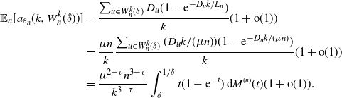 \begin{equation}
\begin{aligned}[b]
{{\mathbb{E}}_n [{a_{\varepsilon_n}(k,W_n^k(\delta))}]}&=\frac{ \sum_{u\in W_n^k(\delta)}D_u(1-{{\rm e}}^{-D_uk/L_n})}{k} (1+{\mathrm{o}}(1))\\
&=\frac{\mu n}{k}\frac{ \sum_{u\in W_n^k(\delta)}\frac{D_uk}{(\mu n)}(1-{{\rm e}}^{-D_uk/(\mu n)})}{k} (1+{\mathrm{o}}(1))\\
&=\frac{\mu^{2-\tau} n^{3-\tau}}{k^{3-\tau}}\int_{\delta}^{1/\delta}t(1-{{\rm e}}^{-t})\,{{\rm d}} {M^{\scriptscriptstyle(n)}}(t) (1+{\mathrm{o}}(1)).
\end{aligned}
\end{equation}
Fix
 $\eta>0$
. Since
 $t(1-{{\rm e}}^{-t})$
is bounded and continuous on
 $[\delta,1/\delta]$
, we can find
 $m<\infty $
, disjoint intervals
 $ (B_i)_{i\in[m]} $
and constants
 $ (b_i)_{i\in[m]} $
such that
 $\cup B_i = [\delta,1/\delta]$
and
 \begin{equation*}
\bigg|t(1-{{\rm e}}^{-t})-\sum_{i=1}^{m}b_i{{\bf 1}_{\{{t\in B_i}\}}}\bigg|<\eta/\lambda([\delta,1/\delta]),
\end{equation*}
for all
 $t\in[\delta,1/\delta]$
. Because
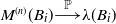 ${M^{\scriptscriptstyle(n)}}(B_i){{\stackrel{{\mathbb{P}}}{\longrightarrow}}} \lambda(B_i)$
for all i,
 \begin{equation*}
\lim_{n\to\infty}{{\mathbb{P}}({|{M^{\scriptscriptstyle(n)}}(B_i)-\lambda(B_i)|>\eta/(m b_i)})}=0.
\end{equation*}
Furthermore,
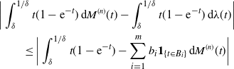 \begin{equation*}\label{eq:Mnlambdasplit}
\begin{aligned}[b]
&\bigg|\int_\delta^{1/\delta}t(1-{{\rm e}}^{-t})\,{{\rm d}} {M^{\scriptscriptstyle(n)}}(t)-\int_\delta^{1/\delta} t(1-{{\rm e}}^{-t})\,{{\rm d}} \lambda(t)\bigg|\\
&\qquad \leq \bigg|\int_\delta^{1/\delta} t(1-{{\rm e}}^{-t})-\sum_{i=1}^mb_i {{\bf 1}_{\{{t\in B_i}\}}}\,{{\rm d}} {M^{\scriptscriptstyle(n)}}(t)\bigg|\\
\end{aligned}
\end{equation*}
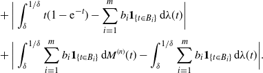 \begin{equation}
\begin{aligned}[b]
& \qquad\quad\, + \bigg|\int_\delta^{1/\delta} t(1-{{\rm e}}^{-t})-\sum_{i=1}^mb_i {{\bf 1}_{\{{t\in B_i}\}}}\,{{\rm d}} \lambda(t)\bigg|\\
&\qquad \quad\, +\bigg|\int_{\delta}^{1/\delta}\sum_{i=1}^mb_i {{\bf 1}_{\{{t\in B_i}\}}}\,{{\rm d}} {M^{\scriptscriptstyle(n)}}(t)-\int_{\delta}^{1/\delta}\sum_{i=1}^mb_i {{\bf 1}_{\{{t\in B_i}\}}}\,{{\rm d}} \lambda(t)\bigg|.
\end{aligned}\end{equation}
Using the fact that
 \[
\int_{\delta}^{1/\delta}{{\bf 1}_{\{{t\in B_i}\}}}\,{{\rm d}}{M^{\scriptscriptstyle(n)}}(t)={M^{\scriptscriptstyle(n)}}(B_i)
\]
yields
 \begin{equation*}
\begin{aligned}[b]
&\bigg|\int_{\delta}^{1/\delta}\sum_{i=1}^mb_i {{\bf 1}_{\{{t\in B_i}\}}}\,{{\rm d}} {M^{\scriptscriptstyle(n)}}(t)-\int_{\delta}^{1/\delta}\sum_{i=1}^mb_i {{\bf 1}_{\{{t\in B_i}\}}}\,{{\rm d}} \lambda(t)\bigg| \\
&\qquad = \bigg|\sum_{i=1}^mb_i({M^{\scriptscriptstyle(n)}}(B_i)-\lambda(B_i))\bigg| \\
& \qquad =\bigg|\sum_{i=1}^m{{\mathrm{o}}_{\scriptscriptstyle{\mathbb{P}}}}(\eta/m)\bigg|={{\mathrm{o}}_{\scriptscriptstyle{\mathbb{P}}}}(\eta).
\end{aligned}
\end{equation*}
Thus, (3.3.2) results in
 \begin{equation*}
\begin{aligned}[b]
&\bigg|\int_\delta^{1/\delta}t(1-{{\rm e}}^{-t})\,{{\rm d}} {M^{\scriptscriptstyle(n)}}(t)-\int_\delta^{1/\delta} t(1-{{\rm e}}^{-t})\,{{\rm d}} \lambda(t)\bigg|\leq \eta\frac{{M^{\scriptscriptstyle(n)}}([\delta,1/\delta])}{\lambda([\delta,1/\delta])} +\eta +{{\mathrm{o}}_{\scriptscriptstyle{\mathbb{P}}}}(\eta).
\end{aligned}
\end{equation*}
Using the fact that
 ${M^{\scriptscriptstyle(n)}}([\delta,1/\delta])={{\mathrm{O}}_{\scriptscriptstyle{\mathbb{P}}}({\lambda([\delta,1/\delta])})}$
proves that
 \begin{equation}
\int_{\delta}^{1/\delta}t(1-{{\rm e}}^{-t})\,{{\rm d}} {M^{\scriptscriptstyle(n)}}(t) {{\stackrel{{\mathbb{P}}}{\longrightarrow}}} \int_{\delta}^{1/\delta}t(1-{{\rm e}}^{-t})\,{{\rm d}} \lambda(t)=c\int_{\delta}^{1/\delta}x^{1-\tau}(1-{{\rm e}}^{-x})\,{{\rm d}} x,
\end{equation}
which together with (27) proves the lemma.
3.3.3. Conditional variance of a (k)
We now show that the variance of
 $a_{\varepsilon_n}(k,W_n^k(\delta))$
is small when conditioning on the degree sequence, so that
 $a_{\varepsilon_n}(k,W_n^k(\delta))$
concentrates around its expected value computed in Lemma 2. Define the event
 \begin{equation*}
\mathcal{K}_n=\{{|{W_n^k(\delta)}|}\leq n(n/k)^{1-\tau}\log(n)\} {.}
\end{equation*}
Since the degrees are i.i.d. samples from (3),
 ${|{W_n^k(\delta)}|}$
is distributed as a binomial with parameters
 $ (n,C(n/k)^{1-\tau}) $
for some constant C. Therefore,
 ${{\mathbb{P}}({\mathcal{K}_n})}\to 1$
.
Leema 4. When
 $n^{(\tau-2)/(\tau-1)}\ll k \ll n^{1/(\tau-1)}/\log(n)$
, on the event
 \[
(D_i)_{i\in[n]}\in \Lambda_n\cap \mathcal{D}_n(\mu n/k)\cap \mathcal{W}_n\cap \mathcal{K}_n,
\]
we have
 \begin{equation*}
\frac{{{\rm Var}_n({a_{\varepsilon_n}(k,W_n^k(\delta))})}}{{{\mathbb{E}}_n [{a_{\varepsilon_n}(k,W_n^k(\delta))}]}^2}\to 0.
\end{equation*}
Proof. We write the variance of
 $a_{\varepsilon_n}(k,W_n^k(\delta))$
as
 \begin{equation}
\begin{aligned}[b]
{{\rm Var}_n({a_{\varepsilon_n}(k,W_n^k(\delta))})} & = \frac{1}{k^2|M_{\varepsilon_n}(k)|^2}\sum_{i,j\in M_{\varepsilon_n}(k)}\sum_{u,v\in W_n^k(\delta)}{D^{\scriptscriptstyle\mathrm{(er)}}}_u{D^{\scriptscriptstyle\mathrm{(er)}}}_w\\
& \quad\, \times ({{\mathbb{P}}_n({X_{iu}=X_{jv}=1})}-{{\mathbb{P}}_n({X_{iu}=1})}{{\mathbb{P}}_n({X_{jv}=1})})
\end{aligned}
\end{equation}
Equation (30) splits into various cases, depending on the size of
 $\{i,j,u,v\}$
. We denote the contribution of
 ${|{\{i,j,u,v\}}|}=r$
to the variance by
 $V^{\scriptscriptstyle{(r)}}(k)$
. We first consider
 $V^{\scriptscriptstyle{(4)}}(k)$
. We can write
 \begin{equation*}
{{\mathbb{P}}_n({X_{iu}=X_{jv}=0})}={{\mathbb{P}}_n({X_{iu}=0})}{{\mathbb{P}}_n({X_{jv}=0\mid X_{iu}=0})}.
\end{equation*}
For the second term, we first pair all half-edges adjacent to vertex i, conditionally on not pairing to vertex u. Then the second term can be interpreted as the probability that vertex j does not pair to vertex v in a new configuration model with
 $\hat{L}_n=L_n-D_i=L_n(1+{\mathrm{O}}(n^{-(\tau-2)/(\tau-1)}\log(n)))$
half-edges, where the new degree of vertex j is reduced by the number of half-edges from vertex i that paired to j,
 $\hat{X}_{ij}$
. Similarly, the new degree of vertex v is reduced by the amount of half-edges from vertex i that paired to v,
 $\hat{X}_{iv}$
. Since
 $\hat{X}_{ij}$
can be dominated by a binomial random variable with parameters
 $D_i,D_j/L_n$
,
 \begin{equation*}
{{\mathbb{P}}({\hat{X}_{ij}> D_jn^{-(\tau-2)/(\tau-1)}})}\leq {{\rm e}}^{-D_jn^{-(\tau-2)/(\tau-1)}/3},
\end{equation*}
and a similar statement holds for
 $\hat{X}_{iv}$
. Let
 $\mathcal{T}_n$
denote the event that
 $\hat{X}_{ij}\leq D_jn^{-(\tau-2)/(\tau-1)}$
and
 $\hat{X}_{iv}\geq D_vn^{-(\tau-2)/(\tau-1)}$
.
 \begin{equation*}
{{\mathbb{P}}_n({X_{jv}=0\mid X_{iu}=0})} = {{\mathbb{P}}_n({X_{jv}=0\mid X_{iu}=0,\mathcal{T}_n})}{{\mathbb{P}}_n({\mathcal{T}_n})}+{\mathrm{O}}({{\mathbb{P}}_n({\mathcal{T}_n^c})}).
\end{equation*}
On the event
 $\mathcal{T}_n$
the new degree of vertex j is
 $\hat{D}_j=D_j(1+{\mathrm{O}}(n^{-(\tau-2)/(\tau-1)}))$
, and a similar statement holds for vertex v. Furthermore, since
 $i,j\in M_{\varepsilon_n}(k)$
,
 $n^{(\tau-2)/(\tau-1)}\ll D_i,D_j \ll n^{1/(\tau-1)}$
and since
 $u,v\in W_n^k(\delta)$
,
 $n^{(\tau-2)/(\tau-1)}\ll D_u,D_v \ll n^{1/(\tau-1)}$
as well. Thus,
 \begin{align*}
{{\mathbb{P}}_n({\mathcal{T}_n^c})}& ={\mathrm{O}}( {{\rm e}}^{-D_jn^{-(\tau-2)/(\tau-1)}}+ {{\rm e}}^{-D_vn^{-(\tau-2)/(\tau-1)}}) ={\mathrm{o}}( {{\rm e}}^{-D_jD_v/L_n})
\end{align*}
Furthermore, by (24),
 \begin{align*}
{{\mathbb{P}}_n({X_{jv}=0\mid X_{iu}=0,\mathcal{T}_n})}& = {{\rm e}}^{-\hat{D}_j\hat{D}_v/\hat{L}_n}+{\mathrm{O}}(n^{-(\tau-2)/(\tau-1)}\log(n))\nonumber\\& ={{\rm e}}^{-D_jD_v/L_n}(1+{\mathrm{o}}(1)),
\end{align*}
so that
 \begin{equation*}
\begin{aligned}[b]
{{\mathbb{P}}_n({X_{iu}=X_{jv}=0})}&
& ={{\rm e}}^{-D_iD_u/L_n}\,{{\rm e}}^{-D_jD_v/L_n}(1+{\mathrm{o}}(1)),
\end{aligned}
\end{equation*}
using the fact that
 $D_iD_u, D_jD_v={\mathrm{O}}(n)$
. This results in
 \begin{align*}
{{\mathbb{P}}_n({X_{iu}=X_{jv}=1})}&=1-{{\mathbb{P}}_n({X_{iu}=0})}-{{\mathbb{P}}_n({X_{jv}=0})}+{{\mathbb{P}}_n({X_{iu}=X_{jv}=0})}\nonumber\\& = 1+(-{{\rm e}}^{-\frac{D_u k}{L_n}}-{{\rm e}}^{-\frac{D_v k}{L_n}}+{{\rm e}}^{-\frac{D_uk}{L_n}-\frac{D_vk}{L_n}})(1+{\mathrm{o}}(1))\nonumber\\& = (1-{{\rm e}}^{-D_uk/L_n})(1-{{\rm e}}^{-D_vk/L_n})(1+{\mathrm{o}}(1)),
\end{align*}
where the last equality holds because
 $D_uk=\Theta(n)$
and
 $D_vk=\Theta(n)$
for
 $u,v\in W_n^k(\delta)$
. Since
 $ (1-{{\rm e}}^{-D_uk/L_n})(1-{{\rm e}}^{-D_vk/L_n})\in[\delta f(n),f(n)/\delta]$
for some f(n) when
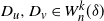 $D_u,D_v\in W_n^k(\delta)$
, these error terms are uniform in
 $i,j\in M_{\varepsilon_n}(k)$
as well as
 $u,v\in W_n^k(\varepsilon)$
. Therefore
 \begin{equation*}
\begin{aligned}[b]
V^{\scriptscriptstyle{(4)}}(k)& = \frac{1}{|M_{\varepsilon_n}(k)|^2
k^2} \sum_{{i,j\in M_{\varepsilon_n}(k)}} \quad \sum_{{u,v\in W_n^k(\delta)}}{D^{\scriptscriptstyle\mathrm{(er)}}}_u{D^{\scriptscriptstyle\mathrm{(er)}}}_v(1-{{\rm e}}^{-D_u k/L_n})(1-{{\rm e}}^{-D_v k/L_n})(1+{\mathrm{o}}(1)) \\
&\quad\, - {D^{\scriptscriptstyle\mathrm{(er)}}}_u{D^{\scriptscriptstyle\mathrm{(er)}}}_v(1-{{\rm e}}^{-D_u k/L_n})(1-{{\rm e}}^{-D_u k/L_n})(1+{\mathrm{o}}(1)) \\
& = \sum_{u,v\in W_n^k(\delta)}{\mathrm{o}}(k^{-2}D_uD_v(1-{{\rm e}}^{-D_u k/L_n})(1-{{\rm e}}^{-D_v k/L_n}))\\
&= {\mathrm{o}}({{\mathbb{E}}_n[{a_{\varepsilon_n}(k,W_n^k(\delta))}]}^2),
\end{aligned}
\end{equation*}
where we replaced
 ${D^{\scriptscriptstyle\mathrm{(er)}}}$
with D as in (25) and the last equality follows from Lemma 2. Since there are no overlapping edges when
 $\{i,j,u,v\}=3$
,
 $V^{\scriptscriptstyle{(3)}}(k)$
can be bounded similarly.
We then consider the contribution from
 $V^{\scriptscriptstyle{(2)}}$
, which is the contribution where the two edges are the same. By Lemma 3, we have to show that this contribution is small compared to
 $n^{6-2\tau}k^{2\tau-6}$
. We bound the summand in (30) as
 \begin{equation*}
\begin{aligned}[b]
D_u^2 ({{\mathbb{P}}_n({X_{iu}=1})}-{{\mathbb{P}}_n({X_{iu}=1})}^2) &\leq D_u^2.
\end{aligned}
\end{equation*}
Thus, using the fact that on
 $\mathcal{A}_n$
,
 $|M_{\varepsilon_n}(k)|\geq 1$
,
 $V^{\scriptscriptstyle{(2)}}$
can be bounded as
 \begin{equation*}
V^{\scriptscriptstyle{(2)}} \leq
\frac{1}{k^2|M_{\varepsilon_n}(k)|^2}\sum_{i\in M_{\varepsilon_n}(k)}\sum_{u\in W_n^k(\delta)}D_u^2
=\frac{1}{k^2|M_{\varepsilon_n}(k)|}\sum_{u\in W_n^k(\delta)}D_u^2
={{\mathrm{O}}({n^2k^{-4}})}{|{W_n^k(\delta)}|}.
\end{equation*}
Thus, on the event
 $\mathcal{K}_n$
,
 \begin{equation*}
V^{\scriptscriptstyle{(2)}}={{\mathrm{O}}_{\scriptscriptstyle{\mathbb{P}}}({n^{4-\tau}k^{\tau-5}})},
\end{equation*}
which is smaller than
 $n^{6-2\tau}k^{2\tau-6}$
when
 $k\gg n^{{(\tau-2)}/{(\tau-1)}}$
, as required.
Proof of Proposition 2. Since
 ${{\mathbb{P}}({\Lambda_n\cap \mathcal{D}_n(\mu n/k)\cap \mathcal{W}_n\cap \mathcal{K}_n})}\to 1$
, Lemma 4 together with the Chebyshev inequality shows that
 \begin{equation*}
\frac{a_{\varepsilon_n}(k,W_n^k(\delta))}{{{\mathbb{E}}_n [{a_{\varepsilon_n}(k,W_n^k(\delta))}]}}{{\stackrel{{\mathbb{P}}}{\longrightarrow}}} 1.
\end{equation*}
Combining this with Lemmas 2 and 3 yields
 \begin{equation*}
\frac{a_{\varepsilon_n}(k,W_n^k(\delta))}{n^{3-\tau}k^{\tau-3}}{{\stackrel{{\mathbb{P}}}{\longrightarrow}}} c\mu^{2-\tau}\int_{\delta}^{1/\delta}x^{1-\tau}(1-{{\rm e}}^{-x})\,{{\rm d}} x.
\end{equation*}
3.3.4. Contributions outside $W_n^k(\delta)$

In this section, we prove Proposition 1 and show that the contribution to
 $a_{\varepsilon_n} (k)$
outside of the major contributing regimes as described in (21) is negligible.
Proof of Proposition 1. We use the fact that
 \[
{\mathbb{P}}_n({X}_{ij}=1)\leq \min\bigg(1,\frac{D_iD_l}{L_n}\bigg).
\]
This yields
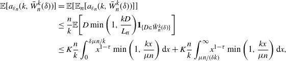 \begin{equation}
\begin{aligned}[b]
{{\mathbb{E}} [{a_{\varepsilon_n}(k,\bar{W}_n^k(\delta))}]}& ={{\mathbb{E}}[{{{\mathbb{E}}_n [{a_{\varepsilon_n}(k,\bar{W}_n^k(\delta))}]}}]}\\
&\leq \frac{n}{k}{{\mathbb{E}}\bigg[{D\min\bigg(1,\frac{kD}{L_n}\bigg){{\bf 1}_{\{{D\in\bar{W}_n^k(\delta)}\}}}}\bigg]}\\
& \leq K \frac{n}{k}\int_{0}^{\delta \mu n/k} \!\!\!\!\!\!\! x^{1-\tau}\min\bigg(1,\frac{k x}{\mu n}\bigg) \,{{\rm d}} x+K\frac{n}{k}\int_{\mu n/(\delta k)}^{\infty}\!\!\!\!\!\!\! x^{1-\tau}\min\bigg(1,\frac{k x}{\mu n}\bigg) \,{{\rm d}} x,
\end{aligned}
\end{equation}
for some
 $K>0$
. For ease of notation, we assume that
 $\mu=1$
. We have to show that the contribution to (31) from vertices u such that
 $D_u<\delta n/k$
or
 $D_u>n/(\delta k)$
is small. First, we study the contribution to (31) for
 $D_u<\delta n/k$
. We can bound this contribution by taking the second term of the minimum, which bounds the contribution as
 \begin{equation*}
\int_{0}^{\delta n/k}x^{2-\tau}\,{{\rm d}} x = \frac{\delta^{3-\tau}}{\tau-3}(k/n)^{\tau-3}.
\end{equation*}
Then, we study the contribution for
 $D_u>n/(k\varepsilon)$
. This contribution can be bounded by taking 1 for the minimum in (31):
 \begin{equation*}
\frac{n}{k}\int_{n/(\delta k)}^\infty x^{1-\tau}\,{{\rm d}} x = \frac{\delta^{\tau-2}}{\tau-2}(k/n)^{\tau-3}.
\end{equation*}
Taking
 $\kappa=\min(\tau-2,3-\tau)>0$
then proves the proposition.
3.4. Expected average nearest-neighbour degree
As in (22), we can write
 \begin{equation}
{{\mathbb{E}}[{a(k,G_n)}]} = {{\mathbb{E}}[{a(k,W_n^k(\delta))}]}+{{\mathbb{E}}[{a(k,\bar{W}_n^k(\delta))}]}.
\end{equation}
By Proposition 1,
 \[
{{\mathbb{E}} [{a(k,\bar{W}_n^k(\delta))}]}/(n/k)^{\tau-3}={\mathrm{O}}(\delta^\kappa).
\]
We now focus on the first term. The expected degree of a neighbour of a randomly chosen vertex of degree k can be written as
 \begin{equation*}
\begin{aligned}[b]
{{\mathbb{E}} [{a(k,W_n^k(\delta))}]} & = {{\mathbb{E}}[{{D^{\scriptscriptstyle\mathrm{(er)}}}_{\mathcal{N}_{V_k}(U)}{{\bf 1}_{\{{D_{\mathcal{N}_{V_k}(U)}\in [\delta,1/\delta]\mu n/k}\}}}}]}\\
& = {{\mathbb{E}}[{D_{\mathcal{N}_{V_k}(U)}{{\bf 1}_{\{{D_{\mathcal{N}_{V_k}(U)}\in [\delta,1/\delta]\mu n/k}\}}}}]}(1+{\mathrm{o}}(1)) {,}
\end{aligned}
\end{equation*}
where
 $\mathcal{N}_{V_k}(U)$
denotes a uniformly chosen neighbour of a vertex of degree k. By (24), we can write the connection probability between a vertex of degree k and a neighbour of degree
 $d\in [\delta,1/\delta]\mu n/k$
as
 $1-{{\rm e}}^{-kd/(\mu n)}(1+{\mathrm{o}}(1))$
. Therefore
 \begin{equation*}
\begin{aligned}[b]
{{\mathbb{E}}[{a(k,W_n^k(\delta))}]}& = (1+{\mathrm{o}}(1))\int_{\delta\mu n/k}^{\mu n/(\delta k)}cx^{1-\tau}(1-{{\rm e}}^{-xk/(\mu n)})\,{{\rm d}} x\\
& =(1+{\mathrm{o}}(1))(n/k)^{3-\tau}c\mu^{2-\tau} \int_{\delta}^{1/\delta}x^{1-\tau}(1-{{\rm e}}^{-x})\,{{\rm d}} x.
\end{aligned}
\end{equation*}
Combining this with (32) and Proposition 1, and letting first
 $n\to\infty$
and then
 $\delta\to 0$
, proves (11).
4. Proofs of Theorem 2 and 3
We now briefly show how the proof of Theorem 1 can be adapted for the rank-1 inhomogeneous random graph and the hyperbolic random graph to prove Theorems 2 and 3. We let
 ${\mathbb{P}}_n$
denote the probability conditioned on the weights in the rank-1 inhomogeneous random graph or conditioned on the radial coordinates in the hyperbolic model.
4.1. Inhomogeneous random graph
First, we show how to prove Theorem 2(i). In the rank-1 inhomogeneous random graph, the degree of vertex i with weight
 $h_i$
satisfies
 $D_i=h_i(1+{{\mathrm{o}}_{\scriptscriptstyle{\mathbb{P}}}}(1))$
when
 $h_i\gg 1$
[Reference Stegehuis, van der Hofstad, van Leeuwaarden and Janssen41]. We condition on the event that the largest weight is smaller than
 $n^{1/(\tau-1)}\log(n)$
, which happens with high probability. Then, when
 $h\ll n^{(\tau-2)/(\tau-1)}/\log(n)$
,
 $p(h,h')=h h'/(\mu n)$
for all vertices. When
 $u\in M_{\varepsilon_n}(k)$
,
 $h_u=k(1+{{\mathrm{o}}_{\scriptscriptstyle{\mathbb{P}}}}(1))$
, so that conditionally on the weight sequence
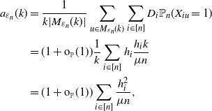 \begin{equation*}
\begin{aligned}[b]
a_{\varepsilon_n} (k)&=\frac{1}{k|M_{\varepsilon_n}(k)|}\sum_{u\in M_{\varepsilon_n}(k)}\sum_{i\in[n]}D_i{{\mathbb{P}}_n({X_{iu}=1})}\\
& =(1+{{\mathrm{o}}_{\scriptscriptstyle{\mathbb{P}}}}(1))\frac{1}{k}\sum_{i\in [n]}h_i\frac{h_i k }{\mu n}\\
& =(1+{{\mathrm{o}}_{\scriptscriptstyle{\mathbb{P}}}}(1))\sum_{i\in[n]}\frac{h_i^2}{\mu n},
\end{aligned}
\end{equation*}
which is equivalent to (20) because the weights are also sampled from (3). This proves Theorem 2(i).
Similarly to (21), we define for the rank-1 inhomogeneous random graph
 \begin{equation}
W_n^{k,\scriptscriptstyle\mathrm{HVM}}(\delta)=\{u \colon h_u\in [\delta\mu n/k, \mu n/(\delta k)] \}.
\end{equation}
Then it is easy to show that Proposition 1 also holds for the rank-1 inhomogeneous random graph with (33) instead of
 $W_n^k(\delta)$
. Because the weights are sampled from (3) and
 ${{\mathbb{P}}_n({X_{ij}=1})}=\min(h_ih_j/(\mu n),1)$
, (31) and therefore also Proposition 1 hold for the rank-1 inhomogeneous random graph as well.
We now sketch how to adjust the proof of Proposition 2 to prove an analogous version for the rank-1 inhomogeneous random graph, which states that
 \begin{equation}
\frac{a_{\varepsilon_n}(k,W_n^{k\scriptscriptstyle\mathrm{HVM}}(\delta))}{(n/k)^{3-\tau}}{{\stackrel{{\mathbb{P}}}{\longrightarrow}}} c \mu^{2-\tau}\int_{\delta}^{1/\delta}x^{1-\tau}\min(x,1)\,{{\rm d}} x.
\end{equation}
Following the proofs of Lemmas 2–4, we see that these lemmas also hold for the rank-1 inhomogeneous random graph if we replace the connection probability of the erased configuration model of
 $1-{{\rm e}}^{-D_iD_j/L_n}$
with
 $\min(h_ih_j/\mu n,1)$
. Note that for the rank-1 inhomogeneous random graph the contribution to (30) from three or four different vertices is 0, because the edge probabilities in the rank-1 inhomogeneous random graph conditioned on the weights are independent. From these lemmas, (34) follows. This then shows similarly to (23) that
 \begin{equation*}
\frac{a_{\varepsilon_n}(k)}{(n/k)^{3-\tau}}{{\stackrel{{\mathbb{P}}}{\longrightarrow}}} c \mu^{2-\tau}\int_{0}^{\infty}x^{1-\tau}\min(x,1)\,{{\rm d}} x =\frac{ c \mu^{2-\tau}}{(3-\tau)(\tau-2)}{,}
\end{equation*}
which proves Theorem 2(ii).
4.2. Hyperbolic random graph
We first provide a lemma that gives the connection probabilities conditioned on the radial coordinates in the hyperbolic random graph. Similarly to (13), let
 $\mathcal{A}_n$
denote the event that the maximal type is smaller than
 $n^{1/(\tau-1)}\log(n)$
. Because t(u) is distributed as (10),
 ${{\mathbb{P}}({\mathcal{A}_n})}\to 1$
.
Leema 5. Denote
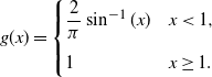 \begin{equation*}
g(x) = \begin{cases}
\frac{2}{\pi} \sin^{-1}(x) & x<1,\\[9pt]
1 & x\geq 1.
\end{cases}
\end{equation*}
Then the probability that u and v are connected in a hyperbolic random graph conditionally on the radial coordinates and on the event
 $\mathcal{A}_n$
, equals
 \begin{equation}
{{\mathbb{P}}_n({X_{uv}=1})}=g(\nu t(u)t(v)/n)(1+{\mathrm{o}}(1)),
\end{equation}
where the
 ${\mathrm{o}}(1)$
term is uniform in u and v.
Proof. Suppose
 $\nu t(u)t(v)/ n\geq 1$
. Then,
 \begin{equation*}
1\leq \frac{\nu t(u)t(v)}{n}=\frac{\nu \,{{\rm e}}^{R}\,{{\rm e}}^{-(r_u+r_v)/2}}{n}=\frac{n}{\nu}\,{{\rm e}}^{-(r_u+r_v)/2},
\end{equation*}
so that
 $r_u+r_v\leq 2\log(n/\nu)=R$
. Thus, by (9),
 \begin{equation*}
\begin{aligned}[b]
\cosh(d(u,v))& = \cosh(r_u)\cosh(r_v)-\sinh(r_u)\sinh(r_v)\cos(\theta_{uv})\\
&\leq \cosh(r_u+r_v) \leq \cosh(R),
\end{aligned}
\end{equation*}
so that the distance between u and v is less than R and u and v are connected.
Now suppose that
 $\nu t(u)t(v)/n<1$
, so that
 $r_u+r_v>R$
. We calculate the maximal value of
 $\theta_{uv}$
such that u and v are connected, which we denote by
 $\theta_{uv}^*$
. When the angle between u and v equals
 $\theta_{uv}^*$
, the hyperbolic distance between u and v is precisely R. Thus, using the definition of the hyperbolic sine and cosine, we obtain
 \begin{equation}
\frac{{{\rm e}}^{R}-{{\rm e}}^{-R}}{2}= \frac{{{\rm e}}^{r_u}-{{\rm e}}^{-r_u}}{2}\frac{{{\rm e}}^{r_v}-{{\rm e}}^{-r_v}}{2}-\frac{{{\rm e}}^{r_u}+{{\rm e}}^{-r_u}}{2}\frac{{{\rm e}}^{r_v}+{{\rm e}}^{-r_v}}{2}\cos(\theta_{uv}^*).
\end{equation}
Since, on the event
 $\mathcal{A}_n$
, the maximal type is at most
 $n^{1/(\tau-1)}\log(n)$
,
 \[
{{\rm e}}^{r_u-r_v}=(t(v)/t(u))^2={{\mathrm{O}}({n^{2/(\tau-1)}\log^2(n)})}
\]
uniformly in u and v. Similarly,
 \[
{{\rm e}}^{r_v-r_u}={{\mathrm{O}}({n^{2/(\tau-1)}\log^2(n)})}
\quad\text{and}\quad
{{\rm e}}^{-r_u-r_v}\leq {{\rm e}}^{r_u-r_v}={{\mathrm{O}}({n^{2/(\tau-1)}\log^2(n)})}
\]
uniformly in u and v. Furthermore,
 ${{\rm e}}^{-R}={\mathrm{O}}(n^{-2})$
, so that (36) becomes
 \begin{equation}
\frac{1}{2}{{\rm e}}^{R} +{\mathrm{O}}(n^{-2})= \frac{1}{4}{{\rm e}}^{r_u+r_v}(1-\cos(\theta_{uv}^*))+{{\mathrm{O}}({n^{2/(\tau-1)}\log^2(n)})}.
\end{equation}
By the definitions of t(u),t(v) and R
 \begin{equation*}
{{\rm e}}^{r_u+r_v}={{\rm e}}^{R}({{\rm e}}^{(r_u+r_v-R)/2})^2={{\rm e}}^{R}\bigg(\frac{n}{\nu t(u)t(v)}\bigg)^2.
\end{equation*}
This yields for (37) that, uniformly in u and v,
 \begin{equation*}
\begin{aligned}[b]
1-\cos(\theta_{uv}^*) & =2\bigg(\frac{\nu t(u)t(v)}{n}\bigg)^2+{{\mathrm{O}}\bigg({n^{\frac{2}{\tau-1}-2}\log^2(n)\frac{\nu ^2t(u)^2t(v)^2}{n^2}}\bigg)}\\
& = 2\bigg(\frac{\nu t(u)t(v)}{n}\bigg)^2(1+{O({n^{-2\frac{(\tau-2)}{\tau-1}}\log^2(n)})}),
\end{aligned}
\end{equation*}
so that
 \begin{equation*}
\theta_{uv}^* = \cos^{-1}(1-2(\nu t(u)t(v)/n)^2)(1+{\mathrm{o}}(1)).
\end{equation*}
Because u and v are connected if their relative angle is at most
 $\theta_{uv}^*$
and the angular coordinates of u and v are sampled uniformly, we obtain that
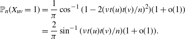 \begin{equation*}
\begin{aligned}[b]
{{\mathbb{P}}_n({X_{uv}=1})} & = \frac{1}{\pi} \cos^{-1}(1-2(\nu t(u)t(v)/n)^2)(1+{\mathrm{o}}(1))\\
& = \frac{2}{\pi} \sin^{-1}(\nu t(u)t(v)/n)(1+{\mathrm{o}}(1)).
\end{aligned}
\end{equation*}
Using this lemma, we now prove Theorem 3.
Proof of Theorem 2. We first focus on
 $k\ll n^{(\tau-2)/(\tau-1)}/\log(n)$
and condition on the event
 $\mathcal{A}_n$
. By [Reference Gugelmann, Panagiotou and Peter22, Section 4.3], for vertex u with radial coordinate
 $r_u$
,
 \begin{equation}
{{\mathbb{E}}_n [{D_u}]}=(n-1)\frac{2\alpha{{\rm e}}^{-r_u/2}}{\pi(\alpha-1/2)}(1+{\mathrm{O}}({{\rm e}}^{-r_u}))= \frac{2\nu(\tau-1)}{\pi(\tau-2)}t(u)(1+{\mathrm{O}}((t(u)/n)^2)),
\end{equation}
where we used that
 $\alpha=(\tau-1)/2$
,
 $t(u) = {{\rm e}}^{-(R-r_u)/2}$
and
 $R=\log(n/\nu)$
. By [Reference Bringmann, Keusch and Lengler12, Theorem 2.7], for every
 $\tau$
and
 $\nu$
, we can interpret the hyperbolic random graph as a variant of the geometric inhomogeneous random graph, defined in [Reference Bringmann, Keusch and Lengler12], where every vertex u has weight
 $w_u=t(u)$
. By [Reference Bringmann, Keusch and Lengler12, Lemma 3.5(ii)],
 $D_u={{\mathbb{E}}_n[{D_u}]}(1+{{\mathrm{o}}_{\scriptscriptstyle{\mathbb{P}}}}(1))$
in geometric inhomogeneous random graphs when
 $w_u=t(u)\gg 1$
. Combining this with (38) we obtain that, in the hyperbolic random graph,
 \begin{equation}
D_u=\frac{2\nu(\tau-1)}{\pi(\tau-2)}t(u)(1+{{\mathrm{o}}_{\scriptscriptstyle{\mathbb{P}}}}(1))
\end{equation}
when
 $1\ll t(u)\ll n$
. When
 $u\in M_{\varepsilon_n}(k)$
,
 $D_u=k(1+{\mathrm{o}}(1))$
. Using (39) then shows that
 \[
t(u)=\frac{\pi(\tau-2)}{2\nu(\tau-1)}k(1+{{\mathrm{o}}_{\scriptscriptstyle{\mathbb{P}}}}(1))
\]
when
 $k\gg 1$
and
 $u\in M_{\varepsilon_n}(k)$
. On the event
 $\mathcal{A}_n$
, the largest type is
 ${{\mathrm{O}}({n^{1/(\tau-1)}\log(n)})}$
. Therefore, if
 $u\in M_{\varepsilon_n}(k)$
, then
 $t(u)t(v)/n={\mathrm{o}}(1)$
for all v. Applying that
 $\sin^{-1}(x)=x+{\mathrm{O}}(x^2)$
to (35) then shows that, for
 $u\in M_{\varepsilon_n}(k)$
,
 \begin{equation*}
{{\mathbb{P}}_n({X_{uv}=1})}= \frac{2\nu t(u)t(v)}{\pi n}(1+{\mathrm{o}}(1)) = \frac{\tau-2}{\tau-1}\frac{k t(v)}{n}(1+{{\mathrm{o}}_{\scriptscriptstyle{\mathbb{P}}}}(1)).
\end{equation*}
Thus, conditionally on the types,
 \begin{equation*}
\begin{aligned}[b]
a_{\varepsilon_n}(k)&=\frac{1}{k|M_{\varepsilon_n}(k)|}\sum_{u\in M_{\varepsilon_n}(k)}\sum_{v\in[n]}D_v{{\mathbb{P}}_n({X_{uv}=1})}\\
&=(1+{{\mathrm{o}}_{\scriptscriptstyle{\mathbb{P}}}}(1))\frac{2\nu(\tau-1)}{\pi(\tau-2) k}\sum_{v\in [n]}t(v)\frac{t(v)k (\tau-2)}{(\tau-1) n} \\
& = (1+{{\mathrm{o}}_{\scriptscriptstyle{\mathbb{P}}}}(1))\sum_{v\in[n]}\frac{2\nu t(v)^2}{\pi n}.
\end{aligned}
\end{equation*}
Combining this with the power-law distribution of the types (10) proves Theorem 3(i), which is the same as Theorem 2(i) where
 $\mu$
is replaced with
 $\pi/(2\nu)$
and
 $c/(\tau-1)$
with 1.
We now investigate the case
 $k\gg n^{(\tau-2)/(\tau-1)}$
. Similarly to (21), we define for the hyperbolic random graph
 \begin{equation*}
W_n^{k,\scriptscriptstyle\mathrm{HRG}}(\delta)=\{u \colon t(u)\in [\delta \zeta n/k,\zeta n/(\delta k)] \}
\end{equation*}
with
 $\zeta=2(\tau-1)/(\pi (\tau-2))$
. Using the fact that
 $2\sin^{-1}(x)/\pi\leq x$
combined with Lemma 5, we obtain
 \begin{equation*}
{{\mathbb{P}}_n({X_{uv}=1})}\leq \min(2\nu t(u)t(v)/(\pi n),1).
\end{equation*}
Combining this with the fact that the t(u)s are sampled from a distribution similar to (3) shows that (31) also holds for the hyperbolic random graph, apart from a multiplicative constant. From there we can follow the same lines as the proof of Proposition 1, so that Proposition 1 also holds for the hyperbolic random graph.
We follow the lines of the proof of Lemma 2, replacing
 $1-{{\rm e}}^{-D_uD_v/L_n}$
with
 $g(\nu t(u)t(v)/n)$
and using (39) to show that
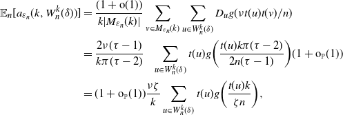 \begin{equation}
\begin{aligned}[b]
{{\mathbb{E}}_n[{a_{\varepsilon_n}(k,W_n^k(\delta))}]}& = \frac{(1+{\mathrm{o}}(1))}{k{|{M_{\varepsilon_n}(k)}|}}\sum_{v\in M_{\varepsilon_n}(k)}\sum_{u\in W_n^k(\delta)}D_ug(\nu t(u)t(v)/n)\\
& =\frac{2\nu (\tau-1)}{k \pi(\tau-2)} \ \ \ \sum_{{u\in W_n^k(\delta)}}t(u)g\bigg(\frac{ t(u)k\pi(\tau-2)}{2n(\tau-1)}\bigg)(1+{{\mathrm{o}}_{\scriptscriptstyle{\mathbb{P}}}}(1))\\
& = (1+{{\mathrm{o}}_{\scriptscriptstyle{\mathbb{P}}}}(1))\frac{\nu\zeta}{k}\sum_{u\in W_n^k(\delta)}t(u)g\bigg(\frac{ t(u)k}{\zeta n}\bigg),
\end{aligned}
\end{equation}
where the error term may be placed in front of the summation since the summand is in
 $n/k[f_1(\delta),f_2(\delta)]$
for some
 $0<f_1(\delta), f_2(\delta)<\infty$
not depending on n. We analyse this expression following the lines of the proof of Lemma 3. We define
 \begin{equation*}
{M^{\scriptscriptstyle(n)}}[a,b] = \frac{1}{\zeta^{1-\tau}n^{2-\tau}k^{\tau-1}}\sum_{u\in[n]}{{\bf 1}_{\{{D_u\in[a,b]\zeta n/k}\}}}
\end{equation*}
similarly to (26). From there, we follow the lines of the proof of Lemma 3, again replacing the connection probability
 $1-{{\rm e}}^{-D_iD_j/(\mu n)}$
of the erased configuration model with
 $g(\nu t(u)t(v)/n)$
and replacing the constant c from (3) with its equivalent constant for the hyperbolic model of
 $\tau-1$
(see (10)) and
 $\mu$
by
 $\zeta$
. Then (40) results in
 \begin{equation*}
\begin{aligned}[b]
{{\mathbb{E}}_n[{a_{\varepsilon_n}(k,W_n^{k,\scriptscriptstyle\mathrm{HRG}}(\delta))}]}& =(1+{{\mathrm{o}}_{\scriptscriptstyle{\mathbb{P}}}}(1)) \frac{\nu n\zeta^2}{k^2}\sum_{u\in W_n^k(\delta)}\frac{t(u)k}{n\zeta }g\bigg(\frac{ t(u)k}{\zeta n}\bigg)\\
& =(1+{{\mathrm{o}}_{\scriptscriptstyle{\mathbb{P}}}}(1))\nu \bigg(\frac{ n\zeta}{k}\bigg)^{3-\tau}\int_{\delta}^{1/\delta}tg (t)\,{{\rm d}} {M^{\scriptscriptstyle(n)}}(t).
\end{aligned}
\end{equation*}
Similar steps that prove (29) then show that
 \begin{equation*}
\begin{aligned}[b]
\frac{{{\mathbb{E}}_n[{a_{\varepsilon_n}(k,W_n^{k,\scriptscriptstyle\mathrm{HRG}}(\delta))}]}}{(n/k)^{3-\tau}} & {{\stackrel{{\mathbb{P}}}{\longrightarrow}}} (\tau-1)\nu\zeta^{3-\tau}\int_{\delta}^{1/\delta}x^{1-\tau}g(x)\,{{\rm d}} x .
\end{aligned}
\end{equation*}
Furthermore, because conditionally on the radial coordinates, the probabilities that two distinct edges are present are independent, Lemma 4 also holds for the hyperbolic random graph. This proves an analogous proposition to Proposition 2, which states that
 \begin{equation*}
\begin{aligned}[b]
\frac{a_{\varepsilon_n}(k,W_n^{k,\scriptscriptstyle\mathrm{HRG}}(\delta))}{(n/k)^{3-\tau}} & {{\stackrel{{\mathbb{P}}}{\longrightarrow}}}(\tau-1) \nu\zeta^{3-\tau}\int_{\delta}^{1/\delta}x^{1-\tau}g(x)\,{{\rm d}} x .
\end{aligned}
\end{equation*}
Therefore, steps similar to those that led to (23) then show that
 \begin{equation*}
\frac{a_{\varepsilon_n}(k)}{(n/k)^{3-\tau}}{{\stackrel{{\mathbb{P}}}{\longrightarrow}}}(\tau-1) \nu\zeta^{3-\tau}\int_{0}^{\infty}x^{1-\tau}g(x)\,{{\rm d}} x.
\end{equation*}
Finally,
 \begin{equation*}
\begin{aligned}[b]
\int_{0}^\infty x^{1-\tau}g(x)\,{{\rm d}} x & = \frac{2}{\pi}\int_{0}^{1}x^{1-\tau}\sin^{-1}(x)\,{{\rm d}} x+\int_{1}^\infty x^{1-\tau}\,{{\rm d}} x\\
& = \frac{2}{\pi}\bigg[\frac{x^{2-\tau}\sin^{-1}(x)}{2-\tau}\bigg]_0^1+\frac{1}{\tau-2}\int_{0}^1\frac{x^{2-\tau}}{\sqrt{1-x^2}}\,{{\rm d}} x+\frac{1}{\tau-2}\\
& = \frac{1}{\tau-2}\int_{0}^{1/(2\pi)}\sin(t)^{2-\tau}\,{{\rm d}} t,
\end{aligned}
\end{equation*}
where the last equation uses the substitution
 $t=\sin(x)$
. By [Reference Gradshteyn and Ryzhik21, equation 3.621.5]
 \begin{equation*}
\frac{1}{\tau-2}\int_{0}^{1/(2\pi)}\sin(t)^{2-\tau}\,{{\rm d}} t = \frac{\Gamma({3-\tau}/{2})\Gamma({1}/{2})}{2(\tau-2)\Gamma({4-\tau}/{2})}=\frac{\sqrt{\pi}\Gamma({3-\tau}/{2})}{2(\tau-2)\Gamma({4-\tau}/{2})},
\end{equation*}
where
 $\Gamma$
denotes the gamma function, which finishes the proof of Theorem 3(ii).
Acknowledgements
This work was supported by NWO TOP grant 613.001.451. The author would like to thank Remco van der Hofstad and Johan S. H. van Leeuwaarden for their useful comments.