2. Model

The first generation of agricultural biotechnology introduced IR and HT traits into three principle row crops in order to mitigate crop damage from insects and weeds, respectively. There have been several applications of the IR trait thus far, having been inserted into corn, cotton and soybean.Footnote ³ The most notable trait causes plants to produce the naturally occurring chemical Bacillus thuringiensis (Bt), which is toxic to common agricultural pests like the European corn borer, but harmless to humans and relatively environmentally benign. In producing the toxin, which has been applied to plants for nearly a century and is employed in modern organic farming, GE crop plants fend off pests without chemical applications by farmers. HT crops express tolerance to glyphosates, a class of broad-spectrum, low toxicity herbicides that includes Round-Up, a Monsanto product also employed in residential settings. Such tolerance, introduced into corn, soybeans and canola, allows farmers to more easily control weeds. In the absence of HT varieties, farmers must rely more heavily on pre-emergence weed control, like tilling operations, and on more toxic and narrow spectrum chemicals that can target weeds without impacting the crop plant.

The IR and HT traits can be modeled as damage control agents that reduce the fraction of crop lost to pests. The framework was first introduced by Lichtenberg and Zilberman (Reference Lichtenberg and Zilberman1986) to model pesticide adoption, and subsequently applied to GE by Qaim and Zilberman (Reference Qaim and Zilberman2003). A wide range of applications followed and are reviewed by Qaim (Reference Qaim2009). We apply the generalized framework from Sexton and Zilberman (Reference Sexton and Zilberman2011) to show how adoption boosts supply on the intensive margin through both a gene effect and complementary-input effects, and along the extensive margin by expanding the range of land that can be profitably farmed.

Production occurs on lands that differ only with respect to pest pressure, denoted by n. The pest pressure at a location may be measured by the average number of pests absent the use of any mitigating agents (like pesticide). Farmers have access to two seed technologies indexed by i with i = 0 denoting traditional seed varieties, and i = 1 denoting GE varieties. GE varieties are considered damage control inputs that affect yields only indirectly by reducing the fraction of crops lost to pests, which affects both the mean and risk of production. We assume a Just and Pope (Reference Just and Pope1978) and constant return to scale production function following Just and Zilberman (Reference Just and Zilberman1988). Thus production per unit of land with technology i is denoted by

(1) $$y_i=f\left(z_i\right)g\left(i\semicolon \; x_i\comma \; n\right)+h\left(z_i\comma \; i\semicolon \; x_i\comma \; n\right)\epsilon$$

The deterministic part of the production function is the product of expected potential output f(z _i ), the average output without pest damage, and the expected efficacy of production g(i; x _i , n), the share not lost to pest damage. Expected potential output is a concave function of inputs like fertilizer per unit of land z _i that increases output directly.Footnote ⁴ Expected efficacy g(i; x _i , n), lies between 0 (complete crop destruction) and 1 (no pest damage) and is increasing in pesticide use and decreasing in pest pressure.Footnote ⁵ It is assumed that on average pest damage is lower under the GE technology than under the traditional technology g (0; x, n) < g (1; x, n). The stochastic element of the per unit of land production function, h (z _i , i; x _i , n)ε, is multiplicative in ε, a random variable with zero mean and variance σ². It is assumed that risk is increasing with fertilizer use, i.e., $\displaystyle{\partial h \over \partial z_{i}}\geq 0$ , and the pest infestation $\displaystyle{\partial h \over \partial n}\geq 0$ , and declining with the level of the pesticides use $\displaystyle{\partial h \over \partial x_{i}}\leq 0$ . It is also reasonable to assume that the risk is smaller after adoption of GE technology (Bennett et al., Reference Bennett, Chi-Ham, Barrows, Sexton and Zilberman2013) so that h (z, 0; x, n) > h (z, 1; x, n).

Let p, w and v denote exogenous prices of outputs, pesticides, and productive inputs, respectively.Footnote ⁶ When farmers initially evaluate the GE technology, they assume seed density per hectare to be constant under both technologies, because changes in seeding density is associated with exogenous cultural practices. The seed cost per unit for technology i is denoted by k _i and it is assumed that k ₁ > k ₀, since seed companies assess technology fees for access to proprietary GE varieties.Footnote ⁷

Because of the concern for segregation between GE and non-GE products we assume that a small producer makes a choice between the two. As in Just and Zilberman (Reference Just and Zilberman1988) we assume constant absolute risk aversion, with a coefficient denoted by r, and a normal distribution of risk. Under these conditions, the maximization of expected utility is equivalent to maximization of expected profit adjusted for expected risk cost:

(2) $$V_i= \mathop {\max }\limits_{{z_i}\comma {x_i}} \, p f\left(z_i\right)g\left(i\semicolon \; x_i\comma \; n\right)-wx_i-vz_i-k_i-.5rp^2 \left[h\left(z_i\comma \; i\semicolon \; x_i\comma \; n\right)\right]^2 \sigma^2$$

The first term of V _i is expected revenue, followed by the costs of pesticides, fertilizers and seeds, minus the expected costs of risk – the product of variance of profits multiplied by the marginal cost of risk per unit of variance of profits. Solving this optimization problem, where the optimal outcomes are denoted by z _i * and x _i *, respectively, suggests that the optimal fertilizer level under the ith technology is determined by

(3) $$\displaystyle{\partial f\lpar z_i\rpar \over \partial z_i} g\lpar i\semicolon \; x_i\comma \; n\rpar = v + rp^2 \displaystyle{\partial h \over \partial z_i} h\lpar z_i\comma \; i\semicolon \; x_i\comma \; n\rpar \sigma^2$$

Equation (3) states that optimal level of the fertilizer z _i * is where the marginal contribution of fertilizers to expected revenue is equal to the price of fertilizers plus the marginal increase in risk because of added fertilizer. Comparative static analysis suggests that more fertilizer will be applied with GE than without, z ₁* ≥ z ₀*. Also, as the pest pressure (n) increases, the expected marginal gain from fertilizers declines, and the marginal risk cost of fertilizers increases, so that application of fertilizers declines (dz _i /dn ≤ 0). This impact on fertilizer contributes to the decline of expected profits adjusted for risk with the pest population. Since pest damage increases less under GE, the reduction in fertilizer use as pest pressure increases is lower with GE than without it (dz ₀/dn ≤ dz ₁/dn ≤ 0).

The optimal level of the pesticide x _i * is where the marginal contribution of pesticides to expected revenue is equal to their price less the marginal increase in the cost of risk because of pesticides use, i.e.,

(4) $$\displaystyle{\partial g\lpar i\semicolon \; x_i\comma \; n\rpar \over \partial x_i}f\lpar z_i\rpar = w + rp^2 \displaystyle{\partial h \over \partial x_i}h\left(z_i\comma \; i\semicolon \; x_i\comma \; n\right)\sigma^2.$$

Because GE combats pests, the marginal productivity of the pesticides it substitutes for is smaller for every level of pest damage and, thus, less of these pesticides are applied with GE, i.e., x ₀* ≥ x ₁*. Because the expected marginal gain from pesticides increases and the marginal risk costs of pesticides declines, application of fertilizers increases with pest pressure (dx _i */dn ≥ 0). This increase is likely to be greater with the non-GE (dx ₀/dn ≥ dx ₁/dn), which will further increase its relative costs.

Introduction of GE technology has several effects in comparison to the traditional technology. First, there is a ‘gene’ effect of reducing pest damage. Second, there is a related effect of increasing seed cost. Third, GE induces a substitution effect, reducing pesticides use (altogether we assume that the ‘gene’ effect dominates the substitution effect on pest damage). Finally, there is an indirect (complementarity) effect of increasing fertilizer use. The ‘gene’ effect (net of substitution) is likely to increase (expected) yield and reduce risk.Footnote ⁸ The indirect effect on fertilizers is likely to increase expected yield and risk further. Furthermore, our analysis suggests that since the GE technology is more capable of addressing the pest pressure, the reduction in expected profits adjusted for risk with GE is smaller than without it (dV ₀*/dn ≤ dV ₁*/dn ≤ 0).

The model enables assessment of the impact of risk and risk aversion on various outcome measures. Without risk (σ² = 0) or under risk neutrality (r = 0), conditions (3) and (4) do not include the risk component. That means that under these conditions fertilizer use will increase and use of pesticides will decline.Footnote ⁹ This means higher (expected) yield and higher variance of profits under risk neutrality. This also means that the net gain from adoption of the GE technology with (d(V ₁* − V ₀*)/dn ≥ 0) increases with pest pressure.

Producers adopt the technology that yields the highest expected profits (adjusted for risk). Their problem is solved recursively. First, conditional on seed technology choice and pest pressure, they choose variable inputs (pesticides and fertilizer). Then they choose the seed that yields the highest expected profits, conditional on optimal input use and provided the expected profits are non-negative. Given heterogeneity in pest conditions, adoption follows the threshold model (David, Reference David1969; Feder et al., Reference Feder, Just and Zilberman1985), in which more vulnerable farmers who gain most from a new technology adopt first and aggregate adoption increases over time as the technology improves or costs of adoption fall.

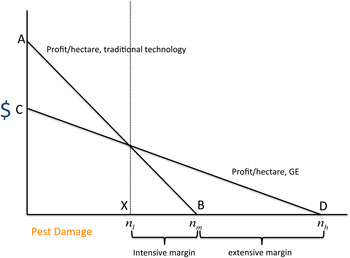
For a given period, the adoption pattern predicted by the model can be depicted as in figure 1. Line segment AB depicts profit per hectare as a function of initial pest pressure under the traditional technology and line segment CD depicts the same for the new technology. At locations with low pest pressure, it is profitable (from now on we will use the term profitable to mean expected profitability adjusted for risk) to farm under either seed technology, but the conventional technology yields higher profits because crop losses are too small to compensate for the technology fee. Thus, below a threshold n _l , farmers produce using the traditional technology. For pest pressure greater than n _l and less than a threshold n _m , it is profitable to use either technology, but higher crop losses from greater pest pressure make damage abatement more valuable so that the new technology yields higher profits. Above n _m and below a high threshold of pest pressure, n _h , it is not profitable to produce under the conventional technology, but it is profitable to produce under the new technology. Above n _h , it is not profitable to produce under any technology; such land is unfarmed.

Figure 1.

Adoption of GE technology.

Notes: The figure plots optimized profits on the y-axis against initial pest pressure on the x-axis.

The area between n _m and n _h is where farmers adopt the new technology and recruit into production land that was too marginal to be profitably farmed under the old technology. This area represents the extensive margin, which we are particularly interested in quantifying. The pest pressure levels n _l , n _m , n _h determine the adoption decision, but the overall magnitude of adoption depends on the amount of land associated with each level of pest damage. If, for example, there is a small amount of hectarage between n _l and n _m and a large amount of land between n _m and n _h , then the intensive margin is small in magnitude while the extensive margin is large. On the other hand, if there is no land with pest damage below n _m , then there is no extensive margin and all the impact is intensive. We return to this issue when we decompose adoption into intensive and extensive margin lands.

3. Estimation

To compute supply, price, land-use and GHG impacts of GE technology, we first compute intensive margin yield impacts from real-world (i.e., non-experimental) production data. While a vast literature estimates yield parameters from farm-level survey or experimental data, we use a cross-country time series of adoption and yield to assess the overall impact of the technology. Our estimates can be interpreted as the average treatment on the treated effects and are inclusive of all complimentary input effects. One reason that previous work has focused on farm-level data is that, until recently, there have not been enough annual observations with positive adoption levels at the country level to consistently estimate macro yield parameters; however, with initial commercialization in 1996, we now have sufficient ‘treatment’ exposure to estimate impacts from within-country time series variation in GE adoption.

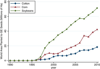
In figure 2, we plot world aggregate adoption by crop over time. Area planted to GE varieties was provided by Graham Brookes, who compiled the data from the International Service for the Acquisition of Agri-Biotech Applications. We can see that GE adoption scaled incredibly fast. In 2010, 15 years after the commercialization of GE technology, GE corn accounted for 42 million ha worldwide across 14 countries, representing 25 per cent of world corn hectarage, GE cotton accounted for 19 million ha worldwide across 10 countries, representing 60 per cent of total cotton hectarage, and GE soybeans accounted for 72 million ha worldwide across nine countries, representing 70 per cent of total soybean hectarage.

Figure 2.

World area planted to GE seeds by crop.

Notes: Authors' own calculation derived from data from Graham Brookes.

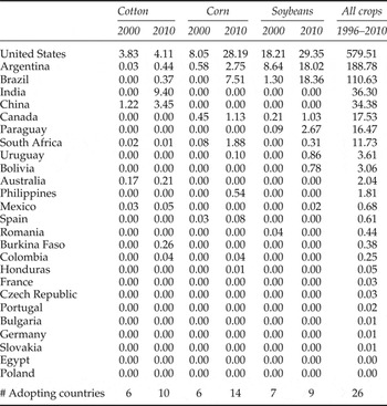
Although GE adoption was rapid, enthusiasm for GE was not shared equally across crops and countries. In table 1, we report adoption by crop and country for the years 2000 and 2010. The table includes all 26 countries that planted any GE seed from 1996 to 2010. Cumulative hectares over the entire adoption period planted to GE seed in any of the three crops is reported in the last column. The US is by far the largest adopter, accounting for 58 per cent of total cumulative adoption, with Argentina and Brazil following with a combined 30 per cent of total adoption, mostly in soybeans. India and China follow next, with a combined 7 per cent of total adoption, mostly in cotton. Outside of these five major adopters, 21 other countries had planted some GE seeds in at least one of the three crops by 2010, though at much lower levels. Our strategy is to exploit this variation in adoption rates over time to estimate yield effects.

Table 1.

Area planted to GE seeds (millions of ha) by country

Notes: Table values represent millions of ha planted to GE technology in the given crop-country-year. Countries are sorted on cumulative adoption over the entire period, which is reported in the last column. Data comes from Graham Brookes.

While country-level data are well-suited to estimating global effects – where ‘global’ means inclusive of all corresponding changes induced by adoption – estimating production function parameters at the aggregate level is problematic. Felipe and Fisher (Reference Felipe and Fisher2003) show aggregate production functions are the weighted sum of micro-level production function that may change over time and reflect spatial and dynamic variability. Thus, estimating parametric coefficients with aggregate data is feasible only under restrictive assumptions. In agriculture, however, a large literature uses macro data to identify nonparametric productivity coefficients (Huffman and Evenson, Reference Huffman and Evenson1992). Following this tradition, we develop a simple method to recover the yield effects of adoption from aggregate national data by decomposing aggregate output into sources of variability in the data. This decomposition approach is similar to the one used in Just et al. (Reference Just, Zilberman, Hochman and Bar-Shira1990). We use the land share of GE as a measure of adoption, while dummy variables allow for variation over crops, countries and time (Feder et al., Reference Feder, Just and Zilberman1985). Statistical power constrains our ability to estimate parameters beyond average effects, but with more data one would be able to further investigate the impact of interaction between factors.

According to equation (1), yield per hectare depends on prices, pest pressure and the technology choice, with no scale effects. The assumption of perfect input and output markets implies price effects are captured by year dummy variables. The time-invariant component of pest pressure is likewise absorbed by country dummies, along with all other time-invariant unobservable determinants of adoption. Remaining agnostic on the precise functional form in (1), the model implies we can write the deterministic component of yield per hectare y _cti in country c, in year t with technology i as the sum of a technology effect β _i country effect α _c and time effect γ _t :

(5) $$y_{cti} = \beta_{i} + \alpha_{c} + \gamma_{t}$$

where γ _t absorbs the intertemporal impact of prices common to all countries and α _c absorbs time-invariant determinants of yield, such as land quality and pest pressure. The structural technology parameters β _i are the parameters of interest.

Total output for a given crop per country-year (Q _ct ) can be written as the sum of output produced with technology i ∈ 0, … I:

(6) $$Q_{ct} = \sum_{i=0}^I Q_{cti} = \sum_{i=0}^I y_{cti}L_{cti}$$

where L _cti is land planted to technology i in country c in time t. Substituting for y _cti , we have:

(7) $$Q_{ct} = \sum_{i=0}^I\left[\beta_{i} + \alpha_{c} + \gamma_{t}\right]L_{cti}$$

Sexton and Zilberman (Reference Sexton and Zilberman2011) estimate the technology parameters with a fixed-effects model:

(8) $$Q_{ct}=\delta_{0} L_{ct} + \delta_{1} L_{ct1}+ \gamma_{t}D_{t} + \alpha_{c}D_{c} + \nu_{ct}$$

with i = 0 denoting traditional seed technology, i = 1 denoting GE technology and D _t and D _c representing dummies for years and countries. While the fixed-effects model (8) controls for country and time-specific unobservables that correlate with adoption, it subsumes country-time specific hectarage deviations in the error term, which correlate with the adoption decision.Footnote ¹⁰ This correlation generates bias in the δ _i s, as they pick up some of the country- and time-specific effects, which multiply the deviations in ν _ct . The direction of the bias is ambiguous, but since bigger countries adopted GE more heavily, it is likely that Sexton and Zilberman (Reference Sexton and Zilberman2011) overestimate the technology effect.

Departing from Sexton and Zilberman (Reference Sexton and Zilberman2011), we divide (7) through by total hectarage and simplify:

(9) $$y_{ct}=\beta_{0} s_{ct0} + \beta_{1} s_{ct1}+ \gamma_{t}+ \phi_{c} + \epsilon_{ct}$$

where y _ct is yield per hectare, s _ct0 and s _ct1 represent shares of hectarage devoted to traditional and GE technology, respectively (again, i = 0 denoting traditional seed technology and i = 1 denoting GE technology), and ε _ct represents an idiosyncratic shock to country-level yield per hectare. Coefficients β₀ and β₁ correspond directly with the structural parameters in (5) and are recovered by estimating (9) via OLS.

In estimating (9), as in Sexton and Zilberman (Reference Sexton and Zilberman2011), the key identification assumption is that country-level adoption shares s _ct0 and s _ct1 are orthogonal to the time-varying shocks ε _ct . Although adoption is not randomly assigned, we argue that unconfoundedness is likely to hold. There are two components of country-level adoption. First, governments have to approve the technology crop by crop. Just et al. (Reference Just, Alston and Zilberman2006) argue that this process is driven largely by political concerns, and hence can be taken as exogenous to unobservable determinants of yield. Second, conditional on government approval, farmers adopt. While it has been shown that GE-adopting farmers are more educated (Crost et al., Reference Crost, Shankar, Bennett and Morse2007), and less risk-averse (Liu, Reference Liu2013), and so should have systematically higher yields, to the extent that unobservable farm or farmer characteristics are time-invariant, they are absorbed by the country dummies. Given endogenous selection at the farm level, our aggregate estimates should be interpreted as average treatment on the treated (ATT) measures, where the ‘treated’ here refer to adopting farmers within adopting countries.

One remaining concern is that time-varying shocks to prices or pest pressure – possibly through weather – could bias estimates in equation (9). But because adoption tends to monotonically increase over the sample, time-varying shocks likely do not influence the adoption decision too much. As Imbens and Wooldridge (Reference Imbens and Wooldridge2007) noted, if s _ct1 > s _cr1 for r < t, then strict exogeneity is a reasonable assumption. Intuitively, if farm-level adoption in period r were induced by a stochastic positive shock to an underlying characteristic, like weather, then a stochastic negative shock to the same characteristic at a time t > r should induce switching back to traditional technology in period t. Since reductions in s _ct1 are rare (only 79 instances out of 4,989 possible country-crop-year observations since 1996), we conclude idiosyncratic shocks to farm or farmer characteristics are unlikely to bias estimates in (9).Footnote ¹¹

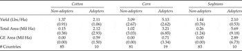
For each GE crop ∈ {corn, cotton, soybeans}, we estimate equation (9) with the same data sources as in Sexton and Zilberman (Reference Sexton and Zilberman2011), although we extend the panel to include more years. Output and area by crop-country-year for 1990–2010 come from FAO Stat. Descriptive statistics are reported by crop and adopting vs. non-adopting countries in table 2, where ‘adopting countries’ have positive GE area for some years for the given crop. The panel for each crop includes all GE adopters and all other 100 top-producing countries.Footnote ¹² We drop observations with 0 output (134 for cotton, 43 for corn, 151 for soybeans) generating an unbalanced panel for each crop. We find in table 2 that adopting countries have higher yields per hectare and higher harvested area in all three crops. Some of the difference is attributable to selection bias into adoption at the country level, while some (potentially) is due to adoption of GE. We control for country fixed effects in order to distinguish between the two.

Table 2.

Summary statistics of adopters and non-adopters by crop (1990–2010)

Notes: Top value in each cell reports the mean over the period, 1990–2010, for the specified country-category. ‘Non-Adopters’ are the countries that report 0 GE planted area throughout the period, while ‘Adopters’ report positive GE planted area in some year over the period. Standard deviations are reported below in parenthesis.

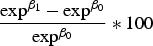
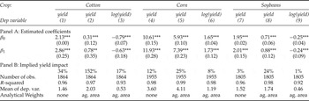
In table 3 we report estimates of equation (9) by crop. The regression coefficients for traditional and GE technology correspond directly with the structural yield parameters β₀ and β₁. In panel A, we begin in columns 1, 4 and 7 by estimating (9) via OLS for cotton, corn and soybeans, respectively. All regressions include year and country fixed-effects. Standard errors are clustered at the country level, so estimates are robust to serial correlation in the error term. For all crops, the coefficients for both traditional and GE yield are individually significant, jointly significant and statistically different, all at the 1 per cent level. The yield effect can be computed as 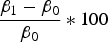$\displaystyle{\beta_{1} -\beta_{0} \over \beta_{0}}\ast100$ and is reported in panel B.Footnote ¹³ We find that the yield effect for cotton is 34 per cent, corn is 12 per cent and soybeans is 3 per cent. By contrast, the yield effects from Sexton and Zilberman (Reference Sexton and Zilberman2011) are 65 per cent for cotton, 45 per cent for corn and 13 per cent for soybeans, again all significant at the 1 per cent level. Our estimates here are smaller than those from per cent Sexton and Zilberman's (Reference Sexton and Zilberman2011) specification, but still mostly larger than other studies in the literature (see Qaim, Reference Qaim2009). This is likely due to the fact that our estimates are based on real-world outcomes, and hence are inclusive of all complementary input effects. The one exception is that we find almost no yield impact of GE soybeans. The small impact on soybeans are possibly explained by ‘yield drag’ resulting from the HT trait. Indeed, much of the benefit from planting HT crops is due not to any inherent yield advantage but the lower cost of managing weeds. Considerable evidence exists that the presence of HT traits in a crop actually lowers yield (Benbrook, Reference Benbrook1999). However, as we show in later sections, even if the yield gain from GE soybeans is low, GE may still boost soybean supply via the extensive margin.

Table 3.

Yield effects of GE Technology

Notes: OLS coefficients are reported by crop for cotton (columns 1–3), corn (columns 4–6) and soybeans (columns 7–9) in panel A. In columns 1–2, 4–5, 7–8, dependents variable is yield per hectare, and in columns 3, 6, and 9, log of yield per hecatre. Standard errors are clustered at the country level and reported in parentheses below. Asterisks indicate statistical significance at the ***1%, **5%, and *10% levels. All regressions are estimated for 1990–2010 and include country fixed effects and year fixed effects. In panel B, yield impact is computed as 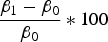$\displaystyle{\beta_{1} - \beta_{0} \over \beta_{0}}\ast100$ when the dependent variable is yield, and 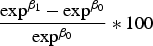$\displaystyle{\exp^{\beta_{1}} - \exp^{\beta_{0}} \over \exp^{\beta_{0}}}\ast100$ when the dependent variable is log yield. Columns 2–3, 5–6, and 8–9 weight by agricultural area.

Next, in columns 2, 5 and 8 of table 3, we estimated weighted regressions to account for difference in country size. Weights correspond to the total agricultural area of the country. Point estimates are still all significant, jointly significant and different from each other. Implied yields increase substantially for all crops, reflecting the correlation between country-level adoption and country size: larger countries adopted more heavily (e.g. US, China, India, Brazil), and their yields increased due to GE, so the average GE effect seems larger when we weight by size. Finally, in columns 3, 6 and 9, we log the dependent variable and weight by size. While the model does not call for logs, it is a common specification in the literature, so we include it for comparison (Lobell et al., Reference Lobell, Schlenker and Costa-Roberts2011).

All three specifications deliver significant GE yield impacts. The specifications reported in columns 1, 4 and 7 provide yield effects estimates that are below those reported in columns 2, 5 and 8 and somewhat above those in columns 3, 6 and 9. As our baseline specification corresponds directly with the statistical model and the results lie between the two other specifications, we prefer the baseline and use the implied yield impacts in columns 1, 4 and 7 to derive supply, price and land-use effects, although we note that other specifications common in the literature (i.e., columns 2–3, 5–6, 8–9) also deliver positive GE yield impacts, though at significantly different magnitudes.

4. Extensive margin

The previous section estimates the increase in yields associated with switching from traditional technology to GE (intensive margin switching), although the adoption model also predicts that GE brings more land into production by extending the range of land that can be profitably farmed. If this relationship is causal, as the model predicts, then output on the extensive margin should be credited to the GE technology, thereby increasing the supply effect of GE seeds. As mentioned in the introduction, we estimate the quantity of new land converted to a given crop since GE was introduced, although we cannot attribute this extensification to the GE technology. We will compute supply and price effects under the bounding assumptions that none (all) of the production on the extensive margin is attributable to GE to understand how important the effect could be.

With plot-level data, the task of decomposing the supply effect into intensive and extensive margins is a simple matter of separating the plots that switched from traditional to GE from those newly planted to GE and summing over the yield increases in each group. Since our data is country level, additional structure is needed to guide the calculation. We appeal to the adoption model from section 2 again to generate the necessary structure.

To illustrate the strategy, consider again figure 1. In some base year – prior to GE entry – the profit curve with traditional technology is given by line segment AB. In a future period, GE becomes available and generates profit curve CD. Suppressing time and country indices, let ΔL ₀ and ΔL ₁ denote the change in traditional and GE hectarage between two periods, with the total change in area ΔL = ΔL ₀ + ΔL ₁. Total hectarage expands in the figure by ΔL = D − B, and GE hectarage expands by ΔL ₁ = D − X, where X indicates the break-even point on GE technology. As described in section 2, the extensive margin, denoted ext, is given by n _h − n _m , or

(10) $$ext =\Delta L = D-B$$

Furthermore, the intensive margin, denoted int, is given by n _m − n _l , or

(11) $$int =\Delta L_0 = B-X$$

Thus, in this case, all we need to compute the intensive and extensive margins are the change in total hectarage ΔL and the change in traditional technology hectarage ΔL ₀, which are figures readily computed from the data.

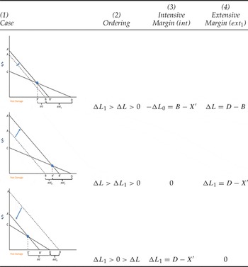
While this simple example illustrates how the adoption model generates enough structure to calculate intensive and extensive hectarage from the aggregate data, the example is not sufficiently general to handle all cases. In particular, we have assumed that the traditional technology profit curve does not change over time. In this case, we have ΔL ₁ > ΔL > 0, and thus equations (10) and (11) yield the intensive and extensive margins. However, in reality, prices, growing conditions and policy all change from year to year, which shifts the traditional technology profit curve. If this profit curve shifts concurrently with the entry of GE technology, we could observe ΔL > ΔL ₁ > 0, for example. In this case, the switchover point X would exceed the x-intercept of the original traditional technology profit curve, implying that all traditional technology hectares from the base year remain traditional technology hectares in the future year; that is, in such a case there is no intensive margin switching. All GE hectares should be counted as extensive margin. Furthermore, it is possible that the traditional technology curve shifts in such that ΔL < 0. In this case, no new lands enter production in the future year, so there can be no extensive margin. In this case, all GE lands should be considered intensive margin.

The general structure for these three cases is presented in table 4. The three cases are distinguished by the ordering of ΔL ₁, ΔL, and 0. In the first case (which includes the first example above), ΔL ₁ > ΔL > 0, there is adoption on both the extensive and intensive margins.Footnote ¹⁴ For this ordering to occur, it is possible that the traditional profit technology curve shifts in or out, but it must be that X′, the observed break-even point in the future period, lies to the left of the initial x-intercept, B. That is, in order for the change in GE hectarage to exceed the change in total hectarage, there must be some intensive margin switching, which implies the break-even point exceeds the initial marginal hectare. In table 4, we illustrate this case in the first row with a small outward shift of the line segment AB to A′B′. The column labeled ‘Ordering’ describes the case, and the columns ‘int’ and ‘ext ₁’ give the calculation of the intensive and extensive margins (‘ext ₁’ indicates extensification with GE technology, while ‘ext ₀’ indicates extensification with traditional technology, and ext = ext ₁ + ext ₀). We find that the intensive margin is computed as the negative of the change in traditional technology hectarage (B − X′), while the extensive margin is computed as the change in total hectarage (D − B). In the second case, illustrated in row 2, we have a large outward shift in AB such that X′ > B. In this case, the total extensive margin is given by the change in total hectarage D − B, but these hectares are divided between extensive margin traditional hectares, ext ₀ = X′ − B, and extensive margin GE hectares ext ₁ = D − X′. There are no intensive margin hectares.Footnote ¹⁵ In the final case, AB shifts in such that the total hectarage decreases. With no new hectares entering production, ext = 0, and any GE hectares come from the intensive margin int = ΔL ₁ = D − X′.

Table 4.

Computation of the intensive vs extensive margins

Notes: Intensive and extensive margin lands are computed based on the ordering of ΔL ₁, ΔL, 0. The three cases are summarized in the different rows here. The first column depicts the case graphically. Column 2 reports the ordering. Column 3 reports the formula for the intensive margin. Column 4 reports the formula for the extensive margin.

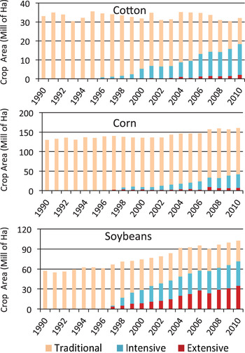
The three cases in table 4 exhaust the possible outcomes when comparing any post-adoption year to the pre-adoption base year.Footnote ¹⁶ Using the data described in section 3, for every country c and year t, we compute the change in total area and GE area (for each crop) between year t and some pre-adoption base year b as ΔL _ct = L _ct − L _cb and ΔL _ct1 = L _ct1 − L _cb1, where the base year is defined as the year immediately prior to the first positive value for GE hectarage for the given country-crop observation. Given ΔL _ct and ΔL _ct1, we classify every country-crop-year as belonging to one of the three cases in table 4 and compute the corresponding intensive and extensive margins according to the formulas in columns 3 and 4.Footnote ¹⁷ We then sum over the given year to generate world hectarage by crop, divided between traditional seed technology, GE intensive margin hectarage and GE extensive margin hectarage. We present results for corn, cotton and soybeans in figure 3.

Figure 3.

World hectarage of GE crops by technology and intensive/extensive margins

Notes: For each crop, cotton, corn, and soybeans, we plot total world area broken down by traditional technology, GE adopted on the intensive margin, and GE adopted on the extensive margin. Area is millions of ha harvested. Intensive margin indicates lands that switched from traditional technology to GE in the same crop, while extensive margin indicates lands that switched from some other crop or purpose into producing the given crop with GE seeds. GE area is divided between intensive margin and extensive margin by the algorithm described in section 4.

In figure 3, we find that for corn, most adoption of GE occurred on the intensive margin, with the extensive margin only accounting for 16 per cent of total GE hectarage in 2010. The share of GE corn hectarage in total corn hectarage is not very large (26 per cent), but because total corn hectarage is so large (the largest world hectarage of all crops) absolute extensification is still substantial. In cotton, overall GE cotton adoption rates are much higher (57 per cent), though mostly still on the intensive margin (only 12 per cent extensive margin). By contrast, adoption of GE soybeans has been high (70 per cent) and more concentrated on the extensive margin than the other crops (49 per cent). As a result, soybean hectarage grew more than 50 per cent since the introduction of the GE seed.

The data show that much of the potential of GE has been realized in cotton and soybean. In the case of cotton, there is a relatively small extensive margin effect, and the adoption of most of the GE has occurred on land previously in production. However, GE cotton is the only GE crop that has been adopted globally, as it did not suffer from bans that apply to corn and soybean. In the case of soybean, the high rate of adoption of GE is attributable to an expansion of the hectarage of the crop (thus the large extensive margin effect), and virtually all of the adoption of GE soybean occurs in the US, Brazil and Argentina. In the case of corn, a majority of corn in the world is located in countries in Europe and Africa that have banned the adoption of GE corn, and therefore overall adoption is below 30 per cent of global hectarage. Because yield per hectare of adopters is higher than that of non-adopters, the GE share of corn is about 43 per cent. Nevertheless, there is a large potential for increased adoption of GE corn if practical bans on the technology are removed.

Breaking down GE area by country, we find that our estimates of extensification are broadly in line with country-specific aggregates. For example, in the case of cotton, 70 per cent of adoption occurred in India and China in 2010, where the total agricultural area has actually declined slightly since the introduction of GE seeds.Footnote ¹⁸ However, we estimate that only 20 per cent and 4 per cent of GE cotton adoption, respectively, for India and China occurred on the extensive margin. With such low GE cotton extensification, it is entirely possible that declining footprints in other crops contribute to overall lower agricultural land base. By contrast, 72 per cent of the extensification effect in soybeans in 2010 is estimated to have come from Brazil and Argentina, where the total agricultural land base has increased since 1995. In fact, 86 per cent of extensification across all crops is estimated to have originated in Brazil, Argentina and the US, where the total agricultural area has increase by a combined 2 million ha since 1995. Thus, while total agricultural area has not increased in all GE-adopting countries, it has increased where our model predicts large extensifications from GE. While a complete analyses of these transition dynamics would require a deeper structural model, it seems the aggregate flows of country-level agricultural area are consistent with our estimates of GE extensification.

As discussed above, the model predicts that the extensive margin draws from lands that were previously of too low a quality (high pest pressure) to farm profitably. In the data, extensive margin lands could draw from marginal land or any other land that was not previously employed in the given crop. Without plot-level data, it is difficult to determine from which uses extensive margin lands are recruited. Given that most of the extensification occurred in Brazil and Argentina, there is some concern that extensive margin lands result from deforestation, rather than the incorporation of marginal lands. In fact, the stock of forested lands has declined since the introduction of GE seeds, but recent research fails to establish a causal link between soybean expansion and deforestation (Hausman, Reference Hausman2012).

An alternative explanation of the extensive margin owes to particularities of the data collection process. Total harvested area from FAO generally counts physical plots, but the GE data counts plot-seasons, i.e., the number of plot-seasons using GE seeds over the year. Thus, if farmers plant multiple seasons within the year using GE technology, it would look like extensification in the data, although really the physical footprint has not increased. Trigo and Cap (Reference Trigo and Cap2006) attribute some of the 9.9 million-ha expansion of soybean area in Argentina to such ‘double-cropping’ activity.Footnote ¹⁹ It is consistent with our model that GE technology permits double-cropping by extending the range of initial pest pressures accommodated by profitable farm operations. In one example, HT varieties permit control of weeds after the crop plant has emerged from the ground, which speeds up production and allows time for follow-on crops to maturate. A fuller description of land-use change dynamics resulting from GE seeds is the subject of ongoing research.

5. Estimated impacts

What do the intensive and extensive margin mean for supply, prices, land-use and GHG emissions? While it is beyond the scope of this paper to conduct a full general equilibrium analysis, we can assess the magnitudes of these impacts in partial equilibrium in two thought experiments. First, we construct a counterfactual supply curve for each crop assuming that GE technology had not been available in 2010. The impact is the horizontal shift in the supply curve caused by the technology. Then, conditional on assumptions of the elasticity of supply and demand, counterfactual equilibrium quantities and prices are computed. The price impact is the percentage difference between the counterfactual price and observed price. Next, to assess the land-use impacts, we calculate how much more land would have been needed to meet observed 2010 demand if GE technology were not available. Finally, we multiply the land-saving figure by a constant GHG per hectare emission rate to compute averted GHG emissions. All impacts are estimated country by country (for each crop) and then aggregated to global figures. We relegate most of the details to the online appendix and just present the results here.

We define the supply effect as the horizontal shift in the supply curve due to GE technology. Only considering the intensive margin yield impact, the supply effect is the percentage difference between observed supply and the counterfactual supply that would have obtained from planting all harvested lands with the lower-yielding traditional technology. However, if one attributes production on the extensive margin to GE technology as well, then the counterfactual supply should subtract production on extensive margin lands as well. We calculate supply effects under these two bounding cases using both our own estimated yield impacts of from section 3, and a range of other yield impacts from the literature.

As shown in figure A.1 in the online appendix, we find that GE technology increased the supply of corn in 2010 between 5 and 12 per cent based on our preferred yield effects from column 4 of table 3, depending on how much of the extensive margin is attributed to GE. Thus, even though extensive margin lands represent a small share of total GE corn hectarage, accounting for the extensive margin can potentially make a large difference for the supply effect. We also estimate supply effects based on Sexton and Zilberman (Reference Sexton and Zilberman2011) along with all the studies reviewed in Qaim (Reference Qaim2009) and find that our supply effects are usually larger, since our estimated yield effects were larger, but the supply effects computed from other yield estimates still generate significant impacts. Estimates range from 2 to 14 per cent without the extensive margin, and 9–19 per cent with the extensive margin. The notable exceptions are Sexton and Zilberman (Reference Sexton and Zilberman2011) and Yorobe and Quicoy (Reference Yorobe and Quicoy2006), which generate slightly larger supply estimates than ours.

Our estimates imply that GE technology increased the supply of cotton between 15 and 20 per cent in 2010, depending on the extensive margin. These results are shown in figure A.2 in the online appendix. Again, these estimates are larger than what would be implied from the yield effects in the Qaim (Reference Qaim2009) review. Finally, for soybeans, we find that because the estimated yield effect is small and the estimated extensive margin effect is large, almost all of the supply effect comes from the extensive margin. We estimate that the supply effect was only 2 per cent without the extensive margin, but as large as 40 per cent with the full extensive margin.

The supply effect from GE technology can be translated into price effects using a methodology from De Gorter and Zilberman (Reference De Gorter and Zilberman1990) and Alston et al. (Reference Alston, Norton and Pardey1995), where the percentage change in equilibrium price is equal to the supply effect divided by the difference between price elasticity of supply and price elasticity of demand (see online appendix). In our estimates we assume an elasticity of supply to be 0.3, while we allow elasticity of demand be either low (−0.3), or high (−0.5).Footnote ²⁰ For each elasticity scenario, we also vary the assumption on the extensive margin as before. For each of these four scenarios {low elasticity, no extensive margin; low elasticity with extensive margin; high elasticity, no extensive margin; high elasticity, with extensive margin} price effects are computed conditional on yield estimates from section 3, Sexton and Zilberman (Reference Sexton and Zilberman2011), and all the studies reviewed in Qaim (Reference Qaim2009).

In figure A.3 in the online appendix, we find that corn prices would have been between 5–19 per cent higher, depending on the assumption of elasticity and extensive margin effect (using our own yield estimates). The price effects in Yorobe and Quicoy (Reference Yorobe and Quicoy2006) and Sexton and Zilberman (Reference Sexton and Zilberman2011) are higher than our estimates, while other studies are roughly five percentage points lower. We find that in all cases, the estimates are more sensitive to the inclusion of the extensive margin than the assumption of demand elasticity. In figure A.4, we find cotton prices would have been 19–33 per cent higher without GE technology. Again, the estimates are higher using our yield impacts instead of others in the literature, but even low yield estimates as in Traxler and Godoy-Avila (Reference Traxler and Godoy-Avila2004) and Falck-Zepeda et al. (Reference Falck-Zepeda, Traxler and Nelson2000) predict that cotton prices would have been 7–19 per cent higher.Footnote ²¹ Finally, for soybeans, the price effect depends heavily on the extensive margin assumption. Without the extensive margin, the price effect is between 3 and 4 per cent. Including the extensive margin, the price effect is between 50 and 66 per cent.

Lastly, we estimate land-use saving effects and the corresponding GHG emissions savings due to GE technology as the difference between observed hectarage in 2010 and counterfactual hectarage that would be needed to produce the same output without the GE supply effects. In this thought experiment, the impact of the intensive margin is unambiguous: without the yield boost from GE, more lands would have been recruited to meet observed demand. However, the impact of the extensive margin is not clear. If extensive margin lands come from truly marginal lands that could not have been used for anything else, then the extensive margin contributes to GHG savings, because without the GE technology, supply from those marginal lands would have been unavailable and more productive lands would have had to have been converted to agriculture. However, if extensive margin lands come from forest, for example, then their conversion (owing to the GE technology) increases GHG emissions because converting forest to agriculture is highly damaging to the environment. Here, we remain agnostic on the source, and hence GHG impacts of extensive margin lands, and only consider the intensive margin impact. In table A.1 of the online appendix, we estimate the land use savings associated with GE cotton are 6 million ha, or roughly 18 per cent of observed 2010 cotton hectarage. Corn land-use savings equals 5 million ha, or 3 per cent of observed corn hectarage. Finally, soybean land-use savings are small, at less than 2 per cent of total soybean hectarage.

In the last column of table A.1, we translate land-use savings into Gt of averted GHG emissions by multiplying the hectares saved by GHG emissions per hectare of land-use change per year. Searchinger et al. (Reference Searchinger, Heimlich, Houghton, Dong, Elobeid, Fabiosa, Tokgoz, Hayes and Yu2008) estimates that converting land to cropland generates on average (across the world) 11.7 metric tonnes (t) of GHG per ha per year.Footnote ²² The US EPA estimates a similar figure and other studies have also applied the Searchinger et al. (Reference Searchinger, Heimlich, Houghton, Dong, Elobeid, Fabiosa, Tokgoz, Hayes and Yu2008) figure to estimate GHG impacts of various activities (Avery and Avery, Reference Avery and Avery2008; EPA, 2012). Multiplying hectares saved by this GHG impact, we find that across all three crops, GE technology saved 0.15 Gt of GHG emissions in 2010. To put this figure in perspective, the total emissions from all passenger cars in the US in 2010 was roughly 1.28 Gt of GHG,Footnote ²³ which means the land-use savings effect of GE technology was roughly one-eighth the size of all emissions from automobiles in the US.