Implications
For addressing the carrying capacity in arid rangelands during a drought, we investigated the influence of livestock number on livestock condition during the drought accounting for livestock movement. Livestock number does not affect livestock conditions per se, it rather affects the temporal threshold after which livestock begin to experience energy deficit. If the drought is shorter than the threshold, livestock conditions are not negatively affected. If the drought exceeds the threshold, livestock experience energy deficit. The carrying capacity of a rangeland during a drought is the number of animals for which the temporal threshold equals the length of the drought.
Introduction
The carrying capacity is traditionally defined as the density of consumers that can stably co-exist in a long-term equilibrium with their resource (Desta and Coppock, Reference Desta and Coppock2002). A system is at its carrying capacity when the rate of forage production equals the rate of forage consumption (Ellis and Swift, Reference Ellis and Swift1988). Such an equilibrium view cannot be applied to systems where the dynamics of consumers and resource are not reciprocally regulated by feedbacks and, consequently, cannot reach a long-term equilibrium.
In arid rangelands, during droughts, the assumption of equilibrium does not hold (Desta and Coppock, Reference Desta and Coppock2002; Sullivan and Rohde, Reference Sullivan and Rohde2002; Vetter, Reference Vetter2005), because the dynamics of livestock and forage are disjoint (Ellis and Swift, Reference Ellis and Swift1988; Sullivan and Rohde, Reference Sullivan and Rohde2002). Even Illius and O’Connor (Reference Illius and O’Connor1999), who sustain that livestock reach a long-term equilibrium with limiting key resources, acknowledge that within the shorter term of droughts livestock and forage resources dynamics are decoupled. It is then important to re-define in the context of a drought the notion of carrying capacity of rangelands. Following McLeod (Reference McLeod1997), carrying capacity could be conceived as the short-term potential livestock number that can be sustained as a function of the resource available. Such a definition of carrying capacity reframes the problem in a well-defined, time-limited context, when consumers and resources are decoupled. This holds independently on whether the long-term dynamics are of equilibrium or non-equilibrium. Indeed, addressing the carrying capacity of arid rangelands during droughts is crucial, as rangelands provide extensive forage resources for traditional livestock rearing in different parts of the world (Ward, Reference Ward2004), and droughts are important components of rangeland dynamics (Bahre and Shelton, Reference Bahre and Shelton1996; Thurow and Taylor, Reference Thurow and Taylor1999; Heidtschmidt et al., Reference Heidtschmidt, Klement and Haferkamp2005).
A driving research question in assessing the short-term carrying capacity during a drought is as follows (Oba, Reference Oba2001): how does the number of animals affect the livestock conditions during the drought? This question helps to investigate whether animal performance during drought is affected by animal density, or only by abiotic factors. In the literature, there are contrasting answers to this question. Some studies (e.g. Fynn and O’Connor, Reference Fynn and O’Connor2000; Desta and Coppock, Reference Desta and Coppock2002) report equivocal observations where animal number does sometimes affect and sometimes not affect animal conditions during the drought. Oba (Reference Oba2001) reports a weak or absent relation between animal number and livestock condition during the drought, whereas according to Gillson and Hoffman (Reference Gillson and Hoffman2007) density-dependent competition is possible even at low stocking rates. Moreover, according to Shackleton (Reference Shackleton1993), there are communal rangelands that continue to support large numbers of livestock without any negative effects on livestock conditions.
To better understand the role of livestock number for livestock conditions during droughts, we developed a model that captures the basic characteristics of an arid rangeland. First, absence or scarcity of rainfall interrupts the growth of the forage resource (Oba, Reference Oba2001). Second, water, a key resource for livestock, is concentrated in scattered points (Illius and O’Connor, Reference Illius and O’Connor1999). This constrains livestock to move continuously from water (concentrated in points) to forage (which is spatially distributed) and vice versa to drink and forage. As a result, livestock cannot forage far from water points (Chamaillé-Jammes et al., Reference Chamaillé-Jammes, Valeix and Fritz2007; Smit et al., Reference Smit, Grant and Devereux2007). Third, forage is heterogeneously distributed in a rangeland, especially during a drought (Scoones, Reference Scoones1995, Illius and O’Connor, Reference Illius and O’Connor2000; Chamaillé-Jammes et al., Reference Chamaillé-Jammes, Valeix and Fritz2007).
To be able to delineate general principles for assessing carrying capacity, we aimed at a parsimonious model that includes all these basic mechanisms, but is kept as simple as possible. We chose an individual-based approach where livestock units were characterized by their internal status (their energy deficit (ED)) and behavior (foraging and going to drink). We chose a spatially explicit approach to focus on the spatial heterogeneity of forage and water distribution. We used this model to observe how livestock number affected livestock conditions during the course of the drought, describing livestock conditions in terms of their ED, that is the amount of energy livestock units are lacking for fulfilling their energy needs.
Material and methods
For our model, we chose the level of complexity in the ‘Medawar zone’ (Grimm et al., Reference Grimm, Berger, Bastiansen, Eliassen, Ginot, Giske, Goss-Custard, Grand, Heinz, Huse, Huth, Jepsen, Jørgensen, Mooij, Müller, Pe’er, Piou, Railsback, Robbins, Robbins, Rossmanith, Rüger, Strand, Souissi, Stillman, Vabø, Visser and DeAngelis2005). The model includes the elements necessary for the understanding of the carrying capacity during droughts, yet it is as simple as possible so we can understand how patterns emerge from it. We did not address predictive purposes, but we aimed at defining general principles for assessing carrying capacity. The model is individual based and spatially explicit because, for our research question, it is important to track the movement of each livestock unit, to describe heterogeneity in forage distribution and to describe the spatial dislocation of water (single point) and forage (spatially distributed). We based the assessment of carrying capacity on the assumption that if livestock spend more energy than they gain from forage in a day, they experience ED and burn fat reserves. Thus, for each livestock unit, we implemented a simple energy balance. We were interested in investigating the dynamics of the system during a drought, so we made the assumption that forage resources do not grow during the drought and we did not simulate the growing season following the drought. Following the approach of Adler and Hall (Reference Adler and Hall2005), the model simulates with an individual-based approach the movement of livestock that start each day from the water point and then go foraging. Although Adler and Hall (Reference Adler and Hall2005) addressed the distribution of forage as emergent from different grazing strategies of animals, we kept the foraging strategy of livestock very simple and we focused on the livestock performance and on the assessment of carrying capacity.
We describe the model using the standard ODD (Overview, Design concepts and Details) protocol for individual-based models (Grimm et al., Reference Grimm, Revilla, Berger, Jeltsch, Mooij, Railsback, Thulke, Weiner, Wiegand and DeAngelis2006), slightly modified to address the characteristics of our specific model. We give a general description of the model in the ‘Overview’ section, stating the purpose of the model, the main variables, spatial and temporal scales, and describing the process scheduling. In the ‘Design concepts’ section, we explain the main properties of the model (basic concepts, emergent properties, interactions between entities, stochasticity) and we illustrate the quantities we aimed to track along the simulations. Finally, we describe the submodels and the model parameterization in the ‘Details and submodels’ section.
Overview
Purpose, spatial resolution and entities
The purpose of the model was to investigate how livestock number, rangeland conditions and forage distribution affect livestock conditions, and to delineate a principle for assessing optimal herd size in a private rangeland during a drought. We considered a spatial domain discretized in hexagonal cells of radius R of 15 m. We defined the distance between two cells as the distance between their centers, that is
 $15\sqrt 3 $
m. Being hexagonal, cells have the same distance to all the neighboring cells. The entities of the model are the livestock units composing the herd. For this study we refer to cows, which are very common in pastoral systems. Cows move in the rangeland system looking for forage and move to the water point for drinking and resting.
Variables and scales
The cell at the center of the spatial domain contains water, whereas all the other cells contain forage of Potentially Edible Biomass (PEB, measured in kg) characterized by a net energy content ε (MJ/kg). The PEB corresponds to the amount of forage that can be consumed by cows. It is in general less than the total amount of forage in the cell, because the lower part of the standing forage is physically inaccessible to the cows and another part of the forage is lost after cows trample the resource while they graze. For the purpose of our model, we needed to investigate the conditions of the cows. We used the following intuitive rationale: if cows can get all the energy needed to fulfill their energy expenses from forage, they are in good conditions. Otherwise, if cows spend more energy than they can obtain from forage, their conditions get worse. Our choice was to assign to the cows a state variable called ED (MJ), representing the amount of energy that must be obtained to fulfill the energy expenses. Note that the level of fat reserves of cows has a physiological maximum (Illius and O’Connor, Reference Illius and O’Connor2000). ED=0 corresponds to the condition of complete fat reserve. When ED>0, the cows are in need of energy and begin to burn their fat reserve. Cows do not eat when the fat reserves are at the maximum level: this implies that ED cannot be negative. We represented a spatial domain of 1.5km×1.5 km to be sure that, during simulations, cows do not go so far from water to exceed the boundaries of the domain. The basic time step of the model was daily with subdivisions as explained in the next section. The temporal extent of the model was 120 days.
Process overview and scheduling
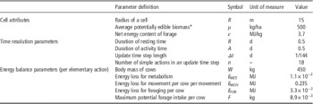
The finest time grain of the model corresponds to the time for a cow to perform an elementary action, which can be move, forage or rest. The action move consists of moving from a cell to a neighboring one; the action forage consists of depleting a certain amount of forage from the cell where the cow is; the action rest occurs when livestock are close to the water point, drink and do not spend a considerable amount of energy. For computational reasons, we chose not to update the model with the same time resolution of an elementary action. For instance, the time required for the action move is very short (<2 min). Simulating a drought with such a time step would require excessive computational time. We decided to organize the time grain hierarchically to meet computational needs and a reasonably precise description of the event scheduling (Figure 1).
Representation of the hierarchical time scheduling of the model. The operator ‘×’ indicates the number of times an action (or a block of actions) is repeated. The two gray boxes represent blocks of actions. Each day is composed of resting time (procedure RestingTime) of length R and activity time of length A, composed of A/Δt procedures ActivityTimeStep of length Δt. The white boxes (within the gray boxes) with continuous contours, represent elementary actions. The white boxes with dotted contours represent instantaneous actions that do not occupy time in the model. In the procedure RestingTime each cow repeats k simple actions move for going to the water point along the shortest path, and rest for the remainder of the RestingTime. M being the number of elementary actions within the procedure RestingTime, the action rest is repeated M−k times. The procedure ActivityTimeStep is composed of n elementary actions. In such a procedure, at the beginning, each cow chooses the target cell where to forage. After that it repeats the procedure move q times going to the target cell along the shortest path, and eventually it repeats the procedure forage n−q times. If the food is depleted, or the cow fills its fat reserves before the end of the n−q elementary forage actions, the action forage corresponds to the action rest. If the target cell coincides with the current cell, q is 0, and the cow forages for n simple actions. If the shortest path to the target cell takes more than n movements, q is n and the cow does not forage. Values of parameters R, A, Δt and n are given in Table 1.

The main time division of the model is between resting time, of length R, and activity time, of length A, with the condition R+A=1 day. During the resting time, cows go to the water point for resting and drinking and do not forage. The time periods dedicated to resting and activity may or may not coincide with night and day, as night grazing can be a common practice in certain pastoral systems (Ayantunde et al., Reference Ayantunde, Fernández-Rivera, Hiernaux, Van Keulen and Udo2002). We simulated the actions and the energy loss of cows during the resting time in one computational step with the procedure RestingTime, described in the ‘Submodels’ section. During the activity time, cows actively look for forage and continuously make decisions about whether to stay in a cell or move to another cell. This implied that the model must be updated frequently during the activity time and required a division of activity time into finer computational steps of length Δt, hereafter called activity time steps. During each of these time steps, cows perform n elementary actions. This means that the time taken to perform an elementary action is Δt/n. We simulated the actions and the energy losses of cows in each activity time step with the procedure ActivityTimeStep, described in the ‘Submodels’ section. In summary, 1 day, in our model, is formed by an initial resting time (procedure RestingTime) and a subsequent succession of A/Δt activity time steps (procedure ActivityTimeStep).
In our scenarios, we simulated a day equally divided by resting time and activity time, so that both of them are 0.5 days. This assumption is in agreement with the observations of Brosh et al. (Reference Brosh, Henkin, Ungar, Dolev, Orlov, Tehuda and Aharoni2006). We chose the length of a day time step Δt=1/144 days, that corresponds to 10 min. For choosing the number n of elementary actions within an activity time step, we based our choice on the velocity of movement of cows from one cell to another. In the elementary action move, cows move from a cell to a neighboring one, covering the distance of
 $15\sqrt 3 $
m in the time taken for an elementary action. Imposing a velocity of movement of 2.90 km/h, given in Loza et al. (Reference Loza, Grant, Stuth and Forbes1992), we estimated a number n=18 of elementary actions, so that each elementary action would take Δt/n~33 s. We acknowledge that cows could move with different velocities in different situations (e.g. when they travel from water to forage, or when they change the grazing cell), however, for this model we needed an average velocity for all the actions to have a uniform time resolution.
Design concepts
Basic concepts
The basic principles underlying this model are the foraging behavior of cows and the link between a cow’s action and its energy balance. The foraging model assumes that cows look for forage during the activity time and come back to the water point for resting and drinking. The energy balance model assumes that cows always consume metabolic energy for sustaining their own vital functions. Cows also consume energy when moving from one cell to another and when they forage. Cows gain energy from forage intake.
Emergence, interactions and stochasticity
The emergent properties of the model are the spatial pattern of consumed forage in the spatial domain and the time trajectory of ED of cows. Individuals interact indirectly by forage removal (scramble competition). When they deplete forage from a cell, they subtract resources from other cows that need to walk more to find forage. The stochasticity here is kept to a minimum. At model initialization, the amount of PEB in each cell is assigned according to a uniform distribution. When cows search forage, they search for the nearest cell with some forage. If two or more cells with forage are at the same distance, the target cell is assigned randomly to the cow.
Observation
In the simulations we observe the average ED of cows. Given the hierarchical organization of computational time, ED can be observed with two temporal resolutions. It can be observed after each computational time step (i.e. after a procedure RestingTime or a procedure ActivityTimeStep), or at the end of each day (after a cycle of a procedure RestingTime and subsequent A/Δt ActivityTimeStep procedures). These two time resolutions contain different information. Observing ED after each computational step gave finer information and described how ED varied within each day. ED at the end of each day represented the daily energy balance. If it was 0, the livestock were able to fulfill the energy needs during the course of that day. In contrast, if it was positive, the livestock spent more energy than they could gain from forage within the course of the day.
Details and submodels
Initialization
We initialized the landscape with a water point in the middle of the spatial domain and PEB randomly distributed in all the other cells. In each cell we allocated a PEB drawn from the uniform distribution on the interval μ±0.1μ, where μ is the average PEB in the rangeland. We simulated three rangeland conditions: μ=400, 500 and 600 kg/ha, respectively, with a net energy content of 3.7 MJ/kg (wheat straw). For each rangeland condition, we ran simulations with different numbers of cows (40 to 200 in increment of 10). Cows were initialized with ED=0, corresponding to the condition of full fat reserve, which can be assumed at the end of the wet season. For each number of cows and for each value of μ, we ran 10 different simulations. These 10 simulations had the same initial average amount of PEB, but with different actual distributions. Thus, comparing these 10 simulations allowed investigating the role of spatial heterogeneity in forage distribution. At the beginning of each simulation, cows were placed in a random neighboring cell of the water point.
Energy expenses and elementary actions
The basic form of energy expense for the cows is metabolic consumption. Cows spend energy for this reason regardless of the action they perform. We defined the parameter E MET (MJ/day) as the amount of energy the cows spend for metabolic consumption in a unit time. We assumed that during the elementary action rest, cows only spend energy for metabolic consumption. Instead, performing the actions move and forage, cows spend additional energy. With the action move, cows move from a cell to a neighboring one. Apart from the energy expense for metabolic rate, the cow spends a fixed amount of energy E MOV (MJ/m) for this movement. With the action forage, cows spend some energy E FOR due to the action of foraging itself, and gain energy from forage. Cows are assigned a potential forage intake F. This intake is potential and not effective, because the effective forage intake is limited by the amount of forage contained in the cell. We stop the forage intake when ED=0, that is, when cows have full fat reserves and do not eat (Illius and O’Connor, Reference Illius and O’Connor2000). The potential forage intake corresponds to the maximum forage-intake capability of cows, the gut-filling effect, depending also on the fiber content of forage. We kept a fixed value of F along the simulations, assuming that the fiber content of forage does not change in time.
The parameters used in the elementary actions depend on the metabolic BW (Demment and van Soest, Reference Demment and van Soest1985; Brosh et al., Reference Brosh, Henkin, Ungar, Dolev, Orlov, Tehuda and Aharoni2006). For this, we considered a BW W equal to 450 kg (known as 1 Animal Unit or 1 Large Stock Unit; Meissner et al., Reference Meissner, Hofmeyr, van Rensburg and Pienaar1983). For the metabolic energy expenses, we used the relationship given in Demment and van Soest (Reference Demment and van Soest1985), corrected to have the energy expressed in MJ/day: E MET=0.293×W0.75. For the energy loss for movement, we considered the value of 0.836 kJ/(kg0.75 m), which was measured by Brosh et al. (Reference Brosh, Henkin, Ungar, Dolev, Orlov, Tehuda and Aharoni2006) averaged across 5 min. We adapted this value to the weight, to the distance between the cells, and to the time resolution of the model. Concerning the energy for foraging E FOR, we considered the value of 91 kJ/(kg0.75 day) as energy per unit metabolic body mass per day (Brosh et al., Reference Brosh, Henkin, Ungar, Dolev, Orlov, Tehuda and Aharoni2006). Concerning the potential forage intake, we considered a total amount of forage that can be ingested in a day equal to 11.25 kg/day as inferred from Prins and Van Langevelde (Reference Prins and Van Langevelde2008) for the BW considered. Such a value is equally distributed within the time steps of the activity time. All the parameters are summarized in Table 1, where their values refer to the time length of an elementary action and to the BW considered.
Parameters of the model with the respective symbols, units of measure and values assigned for the simulations

* Concerning the average potentially edible biomass, we explored three scenarios (400, 500 and 600 kg/ha, respectively).
Procedure RestingTime
During resting time cows reach the water point and rest. We assumed that cows go to the water point following the shortest path and drink while they rest. In the procedure RestingTime, the model updates the ED and the position for each cow. The ED accounts for the metabolic consumption and the movement from the current cell to the water cell. The metabolic consumption is obtained multiplying E MET by the length R of the resting time. Concerning the energy spent for movement, the model counts the number k of movements (from a cell to a neighboring one) separating the current cell from the water cell along the shortest path for each cow. Then the energy for movement is evaluated as k×E MOV. The ED for each cow is then updated with
 $${\rm ED}\leftarrow{\rm ED}{\plus}E_{{{\rm MET}}} {\times}R{\plus}E_{{{\rm MOV}}} {\times}k$$
We assumed that during the activity time, cows forage reasonably close to water. In this way they can always come back to water in a RestingTime computational step. In other words, the time taken from cows to go back to the water point along the shortest path does not exceed the length of resting time R.
Procedure ActivityTimeStep
In an activity time step, cows decide where to forage, walk to that cell and forage. As the model is simplified, we represent an average foraging behavior, which (as in Adler and Hall, Reference Adler and Hall2005) does not include a detailed representation of rumination. As mentioned above, cows spend energy for metabolic consumption, which is E MET×n. At the beginning of the activity time step, cows are assigned their target cell, which is the cell with forage closest to their current cell. In case the current cell has some forage, the target cell coincides with the current cell. If two or more cells with forage have the same distance to the current cell, the target cell is assigned randomly among these cells. Once the target cell is identified, the model identifies the succession of neighboring cells forming the shortest path between the current cell and the target cell for the cows. At this point, the model counts the number m of movements (from a cell to a neighboring one) separating the current cell from the target cell along the shortest path. If m⩾n (=18), the cow cannot reach the target cell within a single activity time step. Thus, the model places the cow n cells away from the current position along the shortest path to the target cell. In this situation, the cow cannot forage, but only spends energy for movement. If m<n, the cow can reach the target cell in m elementary actions and can forage for the remaining n−m elementary actions in the day time step. The effective intake is limited by the potential intake, the amount of forage present in the target cell, and the energy need of the cow. To generalize, we define a number q=min{n, m}, which represents the number of actions move performed by the cow. Consequently, the number n−q represents the number of actions forage performed by the cow. The potential intake of the cow in an activity time step is given by F×(n−q). In this case, if m⩾n, the potential intake is 0, meaning that the cow cannot reach the target cell. If the amount of PEB in the target cell is insufficient to maintain ED=0, the cow consumes all of it, and then has to move to another cell in the next activity time step. Note that the definition of PEB accounts for the fact that not all forage in the cell is consumed by cows. A part of the forage is physically inaccessible to the cows and another is lost due to their trampling. If the ED is sufficiently low, the cow consumes only the forage necessary to bring its ED to 0. Such an amount of forage is given by ED/ε. In summary, the effective intake I is given by
 $$I\,{\equals}\,{\rm min}\left\{ {F{\times}(n{\minus}q),{\rm PEB},{{{\rm ED}} \over {\epsilon}}} \right\}$$
The corresponding energy spent for foraging can be calculated by E FOR×I/F. If I corresponds to F×(n−q), the cow spends all the n−q elementary actions foraging. If I<F×(n−q), the cow forages for a time less than n−q and the energy for foraging is depleted proportionally.
The ED is thus updated as follows:
 $${\rm ED}\leftarrow{\rm ED}{\plus}E_{{{\rm MET}}} {\times}n{\plus}E_{{{\rm MOV}}} {\times}q{\plus}E_{{{\rm FOR}}} {\times}I/F{\minus}{\epsilon}{\times}I$$
Before computing equation (2) the model adds the energetic expenses to ED. This way, if the cow finds in the target cell enough forage to satisfy the resulting energy needs, its ED becomes 0 with equation (3). In case the food in the cell finishes or the ED reaches 0 before the end of the ActivityTimeStep, the cow stops grazing and spends only metabolic energy. This, in fact, corresponds to the action rest. We assumed that no >20 cows could stay at the same time in a cell. In this procedure, the cows are updated one after another. It can happen that a cow is placed in a cell, but the cell is already filled with the maximum number of cows, or the forage is already completely depleted by other cows computed before in the same time step. In this case the cow does not eat during that activity time step, and is moved to another cell in the next time step. To avoid ordering bias, at each activity time step, the cows are computed each time in a new random order.
Results
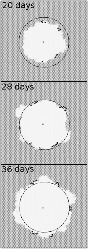
First, we report the details of the results of a simulation with 120 cows and an average PEB of 500 kg/ha to give a basic understanding of the model behavior. Specifically, we report and comment on the spatial patterns emerging during this simulation (Figure 2), and we highlight the main properties of the time trajectory of the average ED of all the cows (Figure 3). Thereafter, we synthesize the results obtained with simulations with different cow numbers (Figure 4) for the same rangeland condition. As expected, cows initially consumed the forage in the proximity of water, and they looked for more and more distant forage, once the nearer forage was consumed (Figure 2). It could be observed that cows (represented as black dots in Figure 2) were distributed in a clustered fashion. The reason is that, at the beginning of the activity time, cows were placed to the cells with forage closest to the water. Being the grazed area not perfectly circular, it could happen that only a few cells were closest to the water point. Cows were then distributed in those few closest cells. During activity time they spread from those cells, but still maintaining a clustered distribution. The number of black dots represented in Figure 2 is far <120 because many cows forage in the same cell (i.e. dots overlap).
Three snapshots of the spatial domain on day 20, day 28 and day 36 of a simulation with 120 cows and initial average potentially edible biomass of 500 kg/ha. The central darker cell represents the water point, the black dots represent cows (more than one cow can be located in the same cell). The white area represents depleted forage. The circle represents the boundary of the threshold area A*. Within area A* cows are able to eat sufficient forage to match the energy they spend, and they do not experience energy deficit. Out of area A*, cows spend more energy than they can gain, and they experience energy deficit. Parameters’ values are given in Table 1.

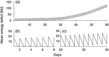
(a) Zoom of the first 60 days of a simulation result in terms of simulated mean energy deficit per cow obtained with 120 cows grazing around the same water point, represented in Figure 2. Panels (b) and (c) show details of the simulation from day 1 to day 8 in (b), and from day 20 to day 30 in (c). Parameters’ values are given in Table 1.

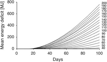
Zoom of the first 100 days of the trajectories of simulated mean energy deficit (ED) observed at a daily time resolution. Trajectories are obtained by averaging 10 simulations with different initial conditions. For each initial condition, each cell was assigned a density of potentially edible biomass uniformly sampled in the interval μ±0.1μ, where μ=500 kg/ha. The number of cows used in each simulated trajectory is indicated at the right of the panel. Parameters’ values are given in Table 1.

The time trajectory of the mean ED of cows was quasi-cyclic (Figure 3a with zooms in Figure 3b and c). During the course of a day (formed by the RestingTime procedure and the subsequent A/Δt ActivityTimeStep procedures) the average ED of cows had an abrupt increase and then a gradual decrease. The first abrupt increase corresponded to the procedure RestingTime where cows spend energy for movement and metabolic consumption; the subsequent gradual decrease corresponded to the energy gained during the activity time with the procedures ActivityTimeStep. The energy gain was due to forage consumption and was limited by forage availability, gut-filling effect and activity time energy expenses (metabolic consumption, movement, foraging).
In the first days of the simulation, ED reached 0 before the end of the day (Figure 3b). This means that the cows could forage enough to neutralize their energy losses. Through the course of the simulation, ED reached 0 later and later within a day, until a certain point where it did not reach 0 before the end of the day (Figure 3c). Thereafter, at the end of each day, ED was positive and became progressively larger (see the final part of Figure 3a). This means that cows could not compensate for the energy losses with forage intake within the course of a day. We highlight that, as a main property within a simulation, there is a time threshold t*. Before such a threshold, the mean ED of cows reached 0 by the end of a day. After the threshold is reached, ED could not reach 0 by the end of a day, but reached greater ED values each successive day.
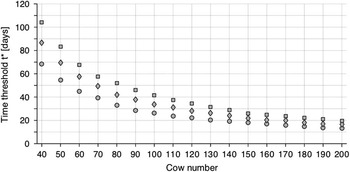
For a synthetic representation of the simulations with different cow numbers, we considered two main properties of the trajectories of mean ED. First, we decided to represent, for each day, only the final value of ED (instead of representing also the trajectory within the course of the day). If this value is 0, it means that cows were capable of fulfilling the energy expenses within the day. If this value is positive, it means that cows consumed more energy than they gained from forage. For each simulation, ED was 0 until the time threshold t*, then it began to increase. For increasing livestock number, the time threshold was smaller, and the increase in ED after the threshold was faster (Figure 4). Second, we considered the time threshold t*, after which the ED began to increase. The time threshold t* decreased with increasing livestock numbers and with worsening rangeland conditions (Figure 5). The SD of the time threshold was always very low (<2 days).
Time threshold t* v. number of cows composing the herd. The time threshold t* represents the time after which the mean energy deficit at the end of each day is >0, and increases monotonically. Simulations are performed for three average densities of potentially edible biomass: 400 kg/ha (circles), 500 kg/ha (diamonds), 600 kg/ha (squares). All other parameter values are given in Table 1. Each time threshold is obtained by averaging the time threshold calculated over 10 simulations. For each value, the SD was<2 days.

Discussion
We developed an individual-based, spatially explicit model for the dynamics of livestock, to assess the carrying capacity in an arid rangeland during a drought. We focused on properties characterizing the behavior of the system: cows need to satisfy hunger and thirst and need to move to water (a single point) and forage (distributed in the spatial domain). We monitored the ED for each cow. When the ED was positive, the cows burned their fat reserves. As the main property describing a simulation, we found that the ED at the end of each day was 0 until a certain time threshold, and then became positive and increased with time. We labeled this time threshold as t* and we investigated how this threshold varied with the number of cows in the simulation and with rangeland conditions. This time threshold could be detected within the length of the simulation chosen (120 days). For parameterizations other than those shown here, it could be possible that longer simulations would be needed.
For interpreting the threshold t*, we considered the spatial dynamics of the model. The model reproduced the general pattern according to which, during a drought, livestock start grazing near the water and then graze at greater distances once the nearest forage is depleted. This is in agreement with observations (James et al., Reference James, Landsberg and Morton1999) and with the outcomes of the model of Adler and Hall (Reference Adler and Hall2005). Day by day, livestock need to walk progressively greater distances from forage to water and vice versa, as the available forage increases its distance from the water point. However, the filling effect and the energy expense during the day (metabolic consumption and forage activity) limit the amount of energy that cows can gain during a day.
We argue that there is an area threshold A* around the water (circle represented in Figure 2). If cows forage within this area threshold, they can replenish all the daily energy losses, as in day 20 (Figures 2 and 3). If cows forage beyond the threshold A*, energy losses due to movement are too high to be replenished by forage intake, as in day 36 (Figures 2 and 3). The time threshold t* corresponds to the time cows take to deplete all the forage within the area threshold A* regardless of how forage is distributed. In the simulation we performed, the time threshold t* coincided with day 28 (Figures 2 and 3). The number of cows influenced the threshold t*. Our results showed that the time threshold decreased with the number of cows. The higher the livestock number is, the faster they consume the forage within the area threshold A*. The time threshold t* decreases in a non-linear way: faster for lower livestock numbers and slower for higher livestock numbers. The greater is the distance they explore, the greater is the area to graze at that distance. As a result, when the cows reach bigger distance, they are slower in consuming the forage at that distance. This is a result of the geometrical characteristics that we considered in our model.
According to our results, the effect of livestock number on condition is not evident while there is forage within the area threshold A*. Thus, livestock number does not affect the ED per se, it rather affects the time at which cows begin to increase their ED, in agreement with Ellis and Swift (Reference Ellis and Swift1988). If cows do not consume the forage in the area A* before the end of the drought (the threshold t* is higher than the length of the drought), they do not experience ED, even with high stocking rates (see also Fynn and O’Connor, Reference Fynn and O’Connor2000). This is likely to occur when area A* contains dense and high-quality forage. In contrast, if cows consume all of the forage in area A* before the end of the drought, they can experience ED and deplete their condition even in small herds (Illius and O’Connor, Reference Illius and O’Connor1999; Gillson and Hoffman, Reference Gillson and Hoffman2007). The consideration of time and area thresholds may help to explain contrasting observations relating livestock number and livestock conditions. If the drought is very long, livestock conditions can get worse even with good rangeland conditions and with low livestock number. If the drought is rather short, livestock might not experience ED even with bad rangeland conditions and high livestock number. Simulations with different initial forage distributions, but sampled from the same uniform distribution, showed very similar values of the threshold t*, with a SD <2 days. This means that the threshold t* was dependent on the average PEB, but not on the spatial distribution within the threshold area A*.
If applied to a private rangeland, the principles delineated by our model can help the rancher allocating the optimal herd size around a water point for a drought. The optimal herd size should be determined so that the time threshold t* corresponds to the length of the drought. Let us consider, for example, a drought of 50 days with a PEB density of 500 kg/ha. The herd size for which the time threshold t* is closest to 50 days is 70 cows, according to the parameters we used (see Figure 5). This means that with >70 cows, the herd is too large. In this case, cows experience ED before the end of the drought. Instead, with <70 cows, the herd is undersized. In this case, cows do not experience ED, but the rancher pays an opportunity cost due to low livestock number. Of course, the length of a drought is often hard to predict; in this case, the rancher needs to be risk-averse and keep the livestock numbers low enough to cope with a long drought (Ward et al., Reference Ward, Saltz and Ngairorue2004; Vetter, Reference Vetter2005). One possible strategy is to consider the probability that a drought lasts for the first 3 months of the dry season, thereafter the second 3 months and so on (Ward et al., Reference Ward, Saltz and Ngairorue2004). Should herd size appear too large after the first 3 months, further herd reductions would be necessary. Alternative, or additional, strategies could include, if feasible, moving the water point where possible to increase access to alternative ranching areas close to forage, promoting herd mobility, watering livestock less often or providing supplementary feed. Communications with Bedouin pastoralists in the Negev desert (Israel) found that a common strategy was to allow their livestock to deplete their forage for one season regardless of ED, and only if the drought continued for a 2nd year, would additional forage be purchased.
We acknowledge that there are some phenomena that are not accounted for in our model, such as land degradation due to trampling, forage senescence, dead tissue loss and decomposition (Illius and O’Connor, Reference Illius and O’Connor2000), more complex physiology of cows, including rumination (van Soest, Reference Van Soest1994), more complex foraging strategies (Adler and Hall, Reference Adler and Hall2005) or a heterogeneous herd composition (e.g. different age classes). We put the complexity of the model in the ‘Medawar zone’ (Grimm et al., Reference Grimm, Berger, Bastiansen, Eliassen, Ginot, Giske, Goss-Custard, Grand, Heinz, Huse, Huth, Jepsen, Jørgensen, Mooij, Müller, Pe’er, Piou, Railsback, Robbins, Robbins, Rossmanith, Rüger, Strand, Souissi, Stillman, Vabø, Visser and DeAngelis2005), as we accounted for only the basic mechanisms occurring during a drought in a rangeland, especially livestock movements from and to water points. This model represented an attempt of addressing the carrying capacity in arid rangeland during a drought. In contrast with the equilibrium view, where carrying capacity is seen as the number of livestock that does co-exist in the long term with the resource, with the basic mechanisms considered, our model revealed temporal and spatial thresholds as crucial elements for determining carrying capacity during droughts.
Acknowledgments
The authors thank the anonymous reviewers that helped to improve this paper. K. W. and D. W. were partly supported by the German Ministry for Education and Research (BMBF) through the IDESSA project (01LL1301A).