2.1. Definition of multi-asset return risk measures

In Equation (1.2), we only sketched the idea of a multi-asset return risk measure; here, we make it precise. As a first step, we introduce all ingredients in our setting. For clarity, we always mention their role in the special setting of return risk measures in Bellini et al. (Reference Bellini, Laeven and Rosazza Gianin2018).

Domain: Risk measures are functionals defined on a particular domain to which we shall refer as model set. It is given by a nonempty subset $\mathcal{C}\subset L^0_{++}$ whose elements we interpret as possible losses an agent faces at a prespecified future time point.

In the example of RRMs from Bellini et al. (Reference Bellini, Laeven and Rosazza Gianin2018), the model set is $L^{\infty}_{++}$ . However, there is no reason to restrict our attention to bounded losses, and we shall work with an arbitrary set $\mathcal{C}$ .

Financial market: Second, we have to describe the payoff that we can create by trading in a financial market. All payoffs generated in this manner form the so-called security set, which is also a nonempty subset $\mathcal{S}\subset L^0_{++}$ . This inclusion imposes the constraint that the generated payoff must be positive, thereby also restricting which trading strategies are deemed admissible. An element of $\mathcal{S}$ is called a security payoff. An important convention to keep in mind is that the random variables in the model set $\mathcal{C}$ are losses, while the security payoffs in ${\mathcal{S}}$ are interpreted as wealth. The price of such a security payoff is given by a map $\pi\colon\mathcal{S}\rightarrow(0,\infty)$ , a so-called pricing map. The fact that $\pi\gt0$ reflects the absence of arbitrage opportunities in the financial market given by $\mathcal{S}$ . Otherwise, there would be an almost surely strictly positive payoff (i.e, $Z\in \mathcal{S}\subset L^{0}_{++}$ ) that we can create at zero or negative costs (i.e., $\pi(Z)\leq 0$ ) by trading on a financial market. This payoff would be an arbitrage opportunity.

In the specific example of RRMs, the security set is based on a single eligible asset, namely a risk-free bank account. In this case, it holds $\mathcal{S}=(0,\infty)$ and $\pi(x)=x$ for all $x\in(0,\infty)$ . Here, however, we aim to allow for other eligible assets like stocks. Therefore, the set $\mathcal{S}$ is introduced as a generic subset of $L^{0}_{++}$ . In particular, unbounded payoffs are possible. For example, $\mathcal{S}$ could represent buy-and-hold strategies in a classical one-period financial market model (see e.g., Föllmer and Schied, Reference Föllmer and Schied2016, Chapter 1), involving investments in a riskless bank account and a stock which has a payoff Y with unbounded support (e.g., Y is lognormally distributed). In this case, $\mathcal{S}=\{a+bY\,;\,a,b\geq 0\text{ with }(a,b)\neq(0,0)\}.$

Acceptability criteria: Next, we formally introduce the set $\mathcal{B}$ from (1.2), which describes if a loss relative to a wealth is acceptable. Here, it is crucial that $\mathcal{B}$ is usually specified without recourse to any financial market, for example, by a regulatory authority. Furthermore, it is already apparent from (1.2) that we need to check if a value of the form $\frac{X}{Z}$ with $X\in\mathcal{C}$ and $Z\in\mathcal{S}$ lies in $\mathcal{B}$ . However, it is well possible that $\frac{X}{Z}\notin \mathcal{C}$ . Therefore, we define $\mathcal{B}$ as a subset of the so-called set of relative losses, which is an independent nonempty subset $\mathcal{K}\subset L^0_{++}$ and which can differ from $\mathcal{C}$ . Then, the relative acceptance set is a nonempty proper subset $\mathcal{B}$ of $\mathcal{K}$ which is monotone, that is,

\begin{align*}\forall\,X\in\mathcal{B}\,\,\forall\,Y\in\mathcal{K}:\quad Y\leq X\quad\implies\quad Y\in\mathcal{B}.\end{align*}

We emphasize that we are interested in values of the form $\frac{X}{Z}$ , where $X \in \mathcal{C}$ and $Z \in \mathcal{S}$ . Acceptability corresponds to small values of $\frac{X}{Z}$ , indicating that Z outperforms X. Broadly speaking, there are two scenarios in which this occurs: either X is small, or X is large but Z is even larger. The first case is clearly desirable. In contrast, the second scenario implies that a large loss may still be considered acceptable.

However, it is important to note that the new risk measure we are about to introduce represents the minimal price of a security payoff Z that renders the loss $\frac{X}{Z}$ relatively acceptable. Therefore, if X is large and Z is even larger, the price for Z should be high. As a result, such a loss is unlikely to be assessed as low risk.

Summing up these ideas, we obtain our new multi-asset version of a return risk measure:

Definition 2.1. A return risk measurement regime is a triplet ${\mathfrak{R}}=(\mathcal B,\mathcal S,\pi)$ consisting of a relative acceptance set $\mathcal B$ , a security set $\mathcal S$ and a pricing map $\pi$ .

Given a return risk measurement regime ${\mathfrak{R}}$ , the associated multi-asset return risk measure (MARRM) $\eta_{\mathfrak{R}}\colon \mathcal{C}\rightarrow[0,\infty]$ is given by

\begin{align*} \eta_{\mathfrak{R}}(X)\;:\!=\inf\left\{\pi(Z)\,;\,Z\in\mathcal{S},\tfrac{X}{Z}\in\mathcal{B}\right\}. \end{align*}

In addition, $Z^{\ast}\in \mathcal{S}$ with $\eta_{\mathfrak{R}}(X)=\pi(Z^{\ast})$ is called an optimal (security) payoff (for X).

The original introduction of RRMs in Bellini et al. (Reference Bellini, Laeven and Rosazza Gianin2018) can be embedded in our general framework by setting $\mathcal{C}=\mathcal{K} = L^\infty_{++}$ and $\mathcal{S} = (0,\infty)$ . In contrast, if we use an arbitrary security set $\mathcal{S}\subset L^{\infty}_{++}$ , it is not ensured a priori that $\frac{X}{Z}\in L^{\infty}_{++}$ unless Z is bounded away from 0. Hence, a choice of $\mathcal{K}=L^{\infty}_{++}$ is not possible any longer without additional assumptions. This motivates us to introduce a notion of compatibility between the model set $\mathcal{C}$ , the set of relative losses $\mathcal{K}$ and the security set $\mathcal S$ . This will be crucial to establish basic properties like monotonicity of the MARRM as an inheritance of the monotonicity of the relative acceptance set $\mathcal B$ (see Lemma 4.1 below). The following new assumption is in place throughout the manuscript:

Assumption 2.3 emphasizes that the set of relative losses $\mathcal{K}$ encompasses fractions $\frac{X}{Z}$ with $X\in\mathcal{C}$ and $Z\in\mathcal{S}$ , thus expressing the size of loss X in terms of wealth Z. Up to scaling, the elements in $\mathcal K$ are random percentages of wealth that are lost, depending on the future state of the economy. In particular, they are dimensionless.

2.2. Representation of MARRMs through multi-asset risk measures

We have already recalled from Bellini et al. (Reference Bellini, Laeven and Rosazza Gianin2018) that there is a close intrinsic connection between return and monetary risk measures. For MARRMs, the counterpart thereof is a natural connection to multi-asset risk measures, which is the topic of the present section.

For our analysis we have to focus on relative acceptance sets defined via return risk measures as in Bellini et al. (Reference Bellini, Laeven and Rosazza Gianin2018). Return risk measures are positively homogeneous by definition. This requires to make the following assumption throughout the present section:

Now we recall the definition of an RRM from Bellini et al. (Reference Bellini, Laeven and Rosazza Gianin2018), but adjust the domain of an RRM.

Now, we develop the desired connection between MARRMs and so-called multi-asset risk measures, thereby generalising the intimate connection between RRMs and monetary risk measures explored in Bellini et al. (Reference Bellini, Laeven and Rosazza Gianin2018). We start with an MARRM and use it to derive a known risk measure formulation. To do so, we introduce sets containing logarithmic transformations of the random variables used in the definition of an MARRM. These sets are the following:

1. (1) Logarithmic model set: $\mathcal{C}_{\log}\;:\!=\left\{\log(X)\,;\,X\in\mathcal{C}\right\}$ ;

2. (2) Set of log-securities: $\mathcal{S}_{\log} \;:\!= \{\log(Z)\,;\, Z\in\mathcal{S}\}$ ;

3. (3) Set of logarithmic relative losses: $\mathcal{K}_{\log}\;:\!=\{\log(K)\,;\,K\in\mathcal{K}\}$ .

From now on, for the rest of this section, we use the following standing assumption:

Now, we recall the well-known definition of an MARM, see for example, Frittelli and Scandolo (Reference Frittelli and Scandolo2006), Scandolo (Reference Scandolo2004).

Definition 2.11. Assume sets $\mathcal{C}^*,\mathcal{S}^*,\mathcal{K}^*\subset L^{0}$ , $\mathcal{A}\subset\mathcal{K}^*$ and a map $\pi^*\colon\mathcal{S}^*\rightarrow\mathbb{R}$ are given. Further, assume that $\mathcal{A}$ is a nonempty proper subset of $\mathcal{K}^{*}$ (nontriviality) such that for all $X\in\mathcal{A}$ , $Y\in\mathcal{K}^*$ with $Y\leq X$ it holds that $Y\in\mathcal{A}$ (monotonicity). The map $\rho_{\mathcal{A},\mathcal{S}^*,\pi^*}\colon\mathcal{C}^*\rightarrow[{-}\infty,\infty]$ defined by

\[\rho_{\mathcal{A},\mathcal{S}^{\ast},\pi^{\ast}}(X)\;:\!=\inf\left\{\pi^{\ast}(Z^{\ast})\,;\,Z^{\ast}\in\mathcal{S}^{\ast},X-Z^{\ast}\in\mathcal{A}\right\}\]

is called a multi-asset risk measure (MARM).

Our next goal is to represent an MARRM via an MARM in the case in which the relative acceptance set is defined via an RRM.

Proposition 2.13. Let $\tilde{\rho}\colon\mathcal{K}\rightarrow(0,\infty)$ be an RRM and ${\mathfrak{R}}=(\mathcal{B}_{\tilde{\rho}}, \mathcal{S}, \pi)$ be a return risk measurement regime. Set $\nu=\log\circ\tilde{\rho}\circ \exp$ , $\mathcal{A}_{\nu}=\{X_{\log}\in\mathcal{K}_{\log}\,;\,\nu(X_{\log})\leq 0\}$ , and $\pi_{\log}=\log\circ\pi\circ \exp$ defined on $\mathcal S_{\log}$ . Then $\eta_{\mathfrak{R}}$ can be represented via the MARM $\rho_{\mathcal{A}_{\nu},\mathcal{S}_{\log},\pi_{\log}}$ as

\[\eta_{\mathfrak{R}} = \exp\circ \rho_{\mathcal{A}_{\nu},\mathcal{S}_{\log},\pi_{\log}}\circ\log.\]

Proof. For $X\in\mathcal{C}$ , we obtain

\begin{align*} \eta_{\mathfrak{R}}(X)&=\inf\left\{\pi(Z)\,;\,Z\in\mathcal{S},\,\tfrac{X}{Z}\in\mathcal{B}_{\tilde{\rho}}\right\}=\inf\left\{\pi(Z)\,;\,Z\in\mathcal{S},\,\tilde{\rho}\big(\tfrac{X}{Z}\big)\leq 1\right\}\\ &=\exp\left(\inf\left\{(\log\circ\pi\circ\exp)(\log(Z))\,;\,Z\in\mathcal{S},\,(\log\circ \tilde{\rho}\circ\exp)\big(\log(X)-\log(Z)\big)\leq 0\right\}\right)\\ &=\exp\left(\inf\left\{\pi_{\log}(L)\,;\,L\in\mathcal{S}_{\log},\,\nu(\log(X)-L)\leq 0\right\}\right)\\ &=\exp\left(\inf\left\{\pi_{\log}(L)\,;\,L\in\mathcal{S}_{\log},\,\log(X)-L\in\mathcal{A}_{\nu}\right\}\right)\\ &=\exp\left(\rho_{\mathcal{A}_{\nu},\mathcal{S}_{\log},\pi_{\log}}(\log(X))\right). \end{align*}

Proposition 2.13 reformulates the MARRM as the exponential of an MARM, applied to a log-transformation. This representation is in line with the considerations in Bellini et al. (Reference Bellini, Laeven and Rosazza Gianin2018), Section 3. Additional care is necessary though. It is common to call $\rho_{\mathcal{A}_{\nu},\mathcal{S}_{\log},\pi_{\log}}$ an MARM only if $\mathcal{C}_{\log}$ is a linear space, $\mathcal{S}_{\log}$ is a linear subspace of $\mathcal{C}_{\log}$ and $\pi_{\log}$ is a strictly positive functional.

Another remarkable feature of representing the MARRM via an MARM is that the domain of the MARM contains log-returns. This contrasts with the original intention of MARMs to measure the risk of monetary loss amounts, see for example, Artzner et al. (Reference Artzner, Delbaen and Koch-Medina2009), Farkas et al. (Reference Farkas, Koch-Medina and Munari2015). The interpretation remains unchanged though: the MARM determines the minimal log-price that is needed to reduce the log-return of our position via the log-return of a security payoff to an acceptable level. Note that, in our context, the MARM is merely an auxiliary function.

For the reader’s convenience, we give a list of all the new abbreviations introduced so far:

• • MARRM: multi-asset return risk measure;

• • MARM: multi-asset risk measure;

• • RRM: return risk measure.

2.3. Connection to risk sharing

Mathematically, risk sharing among a collective of agents is often described by an additive inf-convolution of the involved individual risk measures; see, among many other references, Barrieu and El Karoui (Reference Barrieu and El Karoui2005), Filipović and Svindland (2008), Liebrich and Svindland (Reference Liebrich and Svindland2019). We uncover here that MARRMs exhibit a similar structure, but the additive inf-convolution needs to be replaced by its multiplicative counterpart, which has been studied recently in Aygün et al. (Reference Aygün, Bellini and Laeven2024). More precisely,

(2.1) \begin{align} \eta_{\mathfrak{R}}(X)=\Big(\Pi\otimes \delta^\odot_{\mathcal{B}\cap \frac{\mathcal{C}}{\mathcal{S}}}\Big)(X),\end{align}

where for two functions $f,h\colon\mathcal{C}\rightarrow(0,\infty]$ , the multiplicative inf-convolution is defined by

\begin{align*} (f\otimes h)(X)\;:\!=\inf\{f(Y)h(V)\,;\,Y,V\in\mathcal{C}, YV = X\};\end{align*}

for a set $\mathcal{D}\subset\mathcal{K}$ the multiplicative indicator function $\delta^\odot_{\mathcal{D}}$ is defined by $\delta^\odot_{\mathcal{D}}(X)=1$ if $X\in\mathcal D$ and $\delta^\odot_{\mathcal{D}}(X)=\infty$ otherwise; and where the function $\Pi$ extends the pricing map $\pi$ to all of $L^0_{++}$ by setting $\Pi(X)=\infty$ if $X\notin{\mathcal{S}}$ . This means that the restriction of $\Pi$ to ${\mathcal{S}}$ is $\Pi|_{{\mathcal{S}}}=\pi$ and $\Pi$ acts only as an auxiliary function which allows us to define the multiplicative inf-convolution. This representation shows that an MARRM is obtained by splitting a loss X into a wealth part $Z\in \mathcal S$ generated by a market portfolio and a leverage factor $\frac XZ$ which needs to satisfy a – potentially externally prescribed – constraint formulated by the set $\mathcal B$ . The aggregated risk of this procedure is $\pi(Z)$ for a Z guaranteeing the acceptability of the relative loss $\frac{X}{Z}$ . The trade-off is between creating enough wealth Z to make the relative loss acceptable and minimizing the hedging costs $\pi(Z)$ . Overall, the MARRM offers a new economic model for risk sharing, as the loss is shared multiplicatively. This is different from the case of an MARM, for which we obtain an additive decomposition of the risk X. Following Definition 2.11 for an MARM, we obtain

(2.2) \begin{align} \rho_{\mathcal{A},\mathcal{S}^{\ast},\pi^{\ast}}(X)&= (\delta_{\mathcal{A}}\,\square\, \Pi^{\ast})(X):\!=\inf\{\delta_{\mathcal{A}\cap(\mathcal{C}^{\ast}-\mathcal{S}^{\ast})}(Y)+\Pi^{\ast}(Z^{\ast})\,|\,Y^{\ast},Z^{\ast}\in L^0,Y^{\ast}+Z^{\ast}=X\}. \end{align}

For a set $\mathcal{D}^{\ast}\subset\mathcal{K}^{\ast}$ the indicator function $\delta_{\mathcal{D}^{\ast}}$ is defined by $\delta_{\mathcal{D}^{\ast}}(X)=0$ if $X\in\mathcal{D}^{\ast}$ and $\delta_{\mathcal{D}^{\ast}}(X)=\infty$ otherwise. The function $\Pi^{\ast}$ extends the pricing map $\pi^{\ast}$ to all of $L^0$ by setting $\Pi^{\ast}(X)=\infty$ if $X\notin{\mathcal{S}}^{\ast}$ .

We illustrate multiplicative risk sharing with a concrete insurance example at the end of Section 3.3. There, we compare US private automobile insurance losses (representing the loss X as input of an MARRM) with portfolio payoffs from a Black–Scholes market (representing the security payoffs of the security set $\mathcal{S}$ ). The risk sharing has two components: an optimal payoff resulting from trading in the Black–Scholes market and a leverage factor that compares the insurance loss to the market portfolio. These components are analyzed separately in Figures 5 and 6. With a view at the representations via multiplicative (for $\eta_{\mathfrak{R}}$ in (2.1)) and additive (for $\rho_{\mathcal{A},\mathcal{S}^{\ast},\pi^{\ast}}$ in (2.2)) inf-convolutions, we see that a theoretical comparison is hard to achieve. Instead, we illustrate the difference between additive and multiplicative risk sharing in the empirical study in the next section.

3.1 US private auto claims

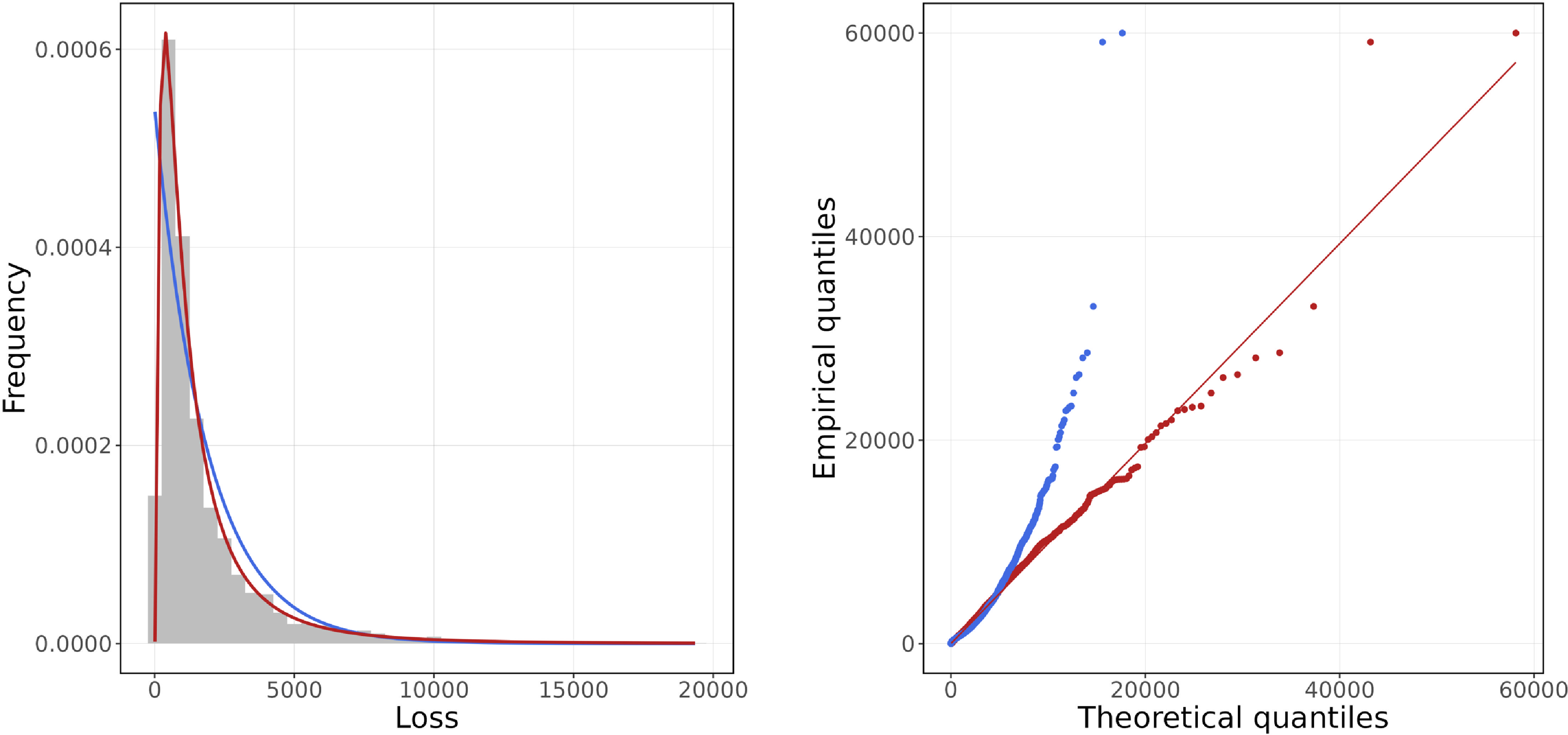
As an example, we use the usprivautoclaim data from the R-package CASdatasets. This dataset contains private motor insurance losses of a US insurance company. On the left-hand side of Figure 1 we present the histogram of the losses. Additionally, we fit a lognormal and an exponential distribution to the data. The quantile-quantile(QQ)-plot on the right-hand side shows that the exponential distribution does not lead to a good fit. In contrast, the lognormal distribution seems to be a reasonable choice. This is line with the literature, see, for example (Wüthrich Reference Wüthrich2024, Section 3.2.3). Furthermore, the lognormal distribution can be used to approximate the total claim amount for small portfolio sizes, see again (Wüthrich Reference Wüthrich2024, Section 4.1.2).

Figure 1.

LHS: Histogram of losses below 20,000 from the usprivautoclaim data. The red, respectively, blue, curve is the density of a lognormal, respectively, exponential, distribution, fitted via method of moments. RHS: QQ-plots of the empirical quantiles against the theoretical ones regarding the fitted lognormal (red) and exponential (blue) distribution.

So, from now on, we assume a risky position that is lognormally distributed, $X\sim\text{LN}(\mu,\sigma^2)$ , where we specifically use the calibrated parameters of the lognormal distribution from Figure 1, $\mu = 6.9686$ and $\sigma = 1.0545$ . In addition, we assume that X is uncorrelated to the stocks. The latter is a meaningful assumption, because losses from the insurance business, such as those from car crashes, are independent of fluctuations on a stock exchange. Under these specifications, we always end up with lognormally distributed relative losses:

(3.2) \begin{align} \frac{X}{Z^{x_0,\xi}_T}\sim \text{LN}\big(\mu-\log(x_0)-\big(\xi^{\intercal}(b-r\boldsymbol{1}) + r -\tfrac{\left\lVert\xi^{\intercal}\Sigma\right\rVert^2}{2}\big)T,\sigma^2+\left\lVert\xi^{\intercal}\Sigma\right\rVert^2 T\big).\end{align}

3.2 Comparison with RRM

We begin by comparing MARRMs with their RRM counterparts. To the best of our knowledge, even in the case of MARMs, there are only few references that illustrate the influence of multiple eligible assets in concrete market setups. For instance, Desmettre et al. (Reference Desmettre, Laudagé and Sass2020) compare monetary risk measures and MARMs in a one-period Black-Scholes setup, that is, no intermediate trading is allowed. Laudagé et al. (Reference Laudagé, Sass and Wenzel2022) compare the two types of risk measures in a balance-sheet model with distributions inspired by the CAPM market model. Finally, Frittelli and Scandolo (Reference Frittelli and Scandolo2006) compare MARMs for different security sets consisting of stochastic processes instead of random variables.

We use the following acceptability criteria for a strictly positive random variable X and a level $\lambda\in(0,1)$ :

1. (1) Value-at-Risk (VaR) criterion: $\exp\left(q^{-}_{\log(X)}(\lambda)\right)\leq 1$ ;

2. (2) Average-Return-at-Risk (ARaR) criterion: $\exp\left(\frac{1}{1-\lambda}\int_{\lambda}^{1}q^{-}_{\log(X)}(u)\textrm{d}u\right) \leq 1$ .

The ARaR is the RRM based on the Expected Shortfall as underlying monetary risk measure, see (Laeven and Rosazza Gianin Reference Laeven and Rosazza Gianin2022, Example 7). Acceptability is captured by the parameter $\lambda\in(0,1)$ .

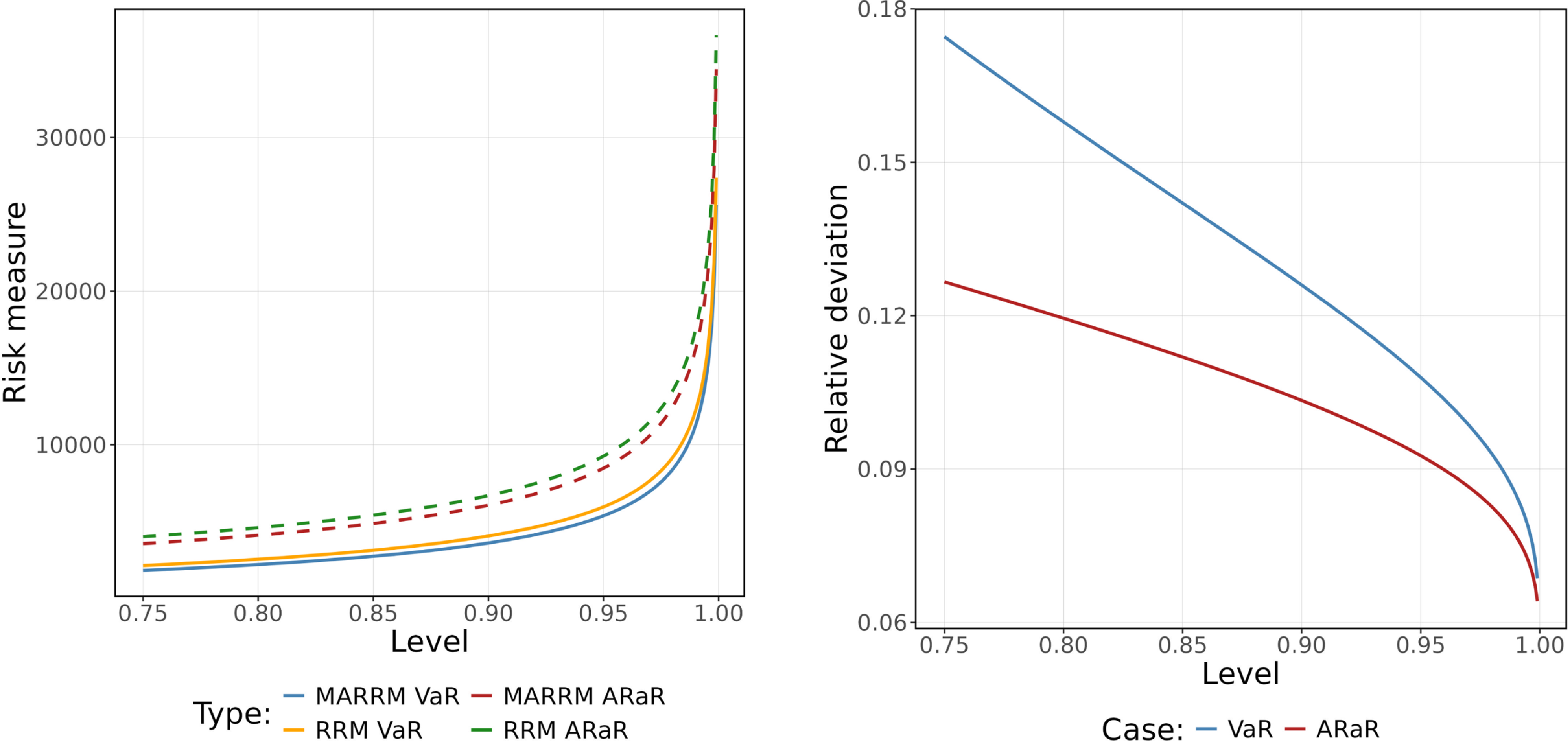
In Figure 2, we compare the MARRM to the RRM at varying levels of the acceptability parameter $\lambda$ . In the left-hand figure, MARRM and RRM values are depicted as functions of $\lambda$ . In the right-hand figure, for VaR- and ARaR-based acceptability criteria, MARRM and RRM are compared in relative terms by looking at the fraction

(3.3) \begin{equation}\frac{\text{RRM}- \text{MARRM}}{\text{MARRM}}\end{equation}

representing the relative deviation of RRM from MARRM. We see that even for large levels, the deviation is above 6%. Hence, the introduction of multiple eligible assets indeed leads to a significant reduction of the minimal hedging costs. Furthermore, the relative deviation in the VaR-case is larger than in the ARaR-case. The gap is smaller for larger levels, which indicates that for such levels the optimal hedging strategies for the MARRMs in the VaR- and ARaR-case are similar.

Figure 2.

LHS: MARRM and RRM for different levels $\lambda$ . RHS: Relative deviation between MARRM and RRM for different levels $\lambda$ based on the same acceptance sets.

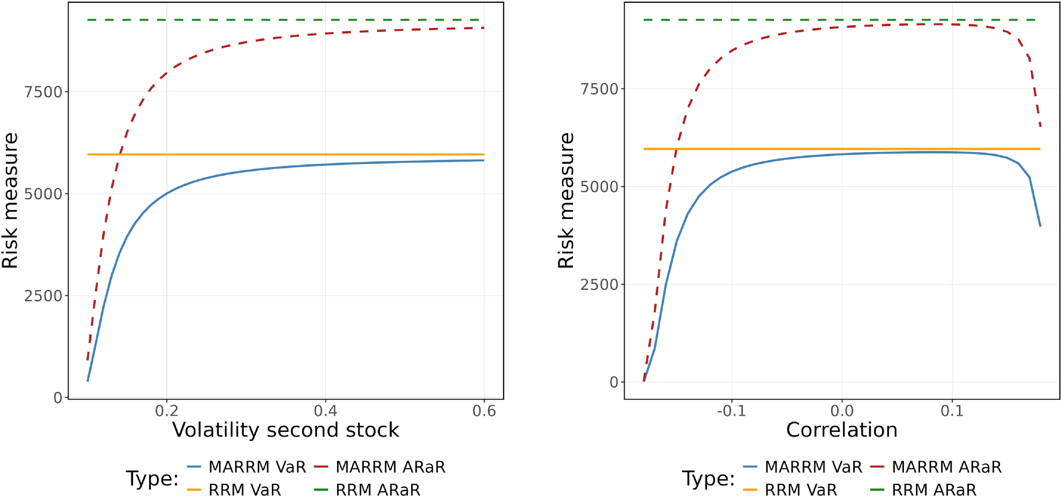
In Figure 3, we test the sensitivity to the chosen parameters. To this effect, we fix $\lambda = 0.95$ and vary the volatility of the second stock $\sigma_{22}$ (left hand side) and the correlation $\sigma_{12} = \sigma_{21}$ of the two stocks (right hand side). The RRM remains unaffected by these changes, as it does not rely on stocks as hedging instruments. Further, we see that the MARRM goes to zero at values for which the matrix $\Sigma$ becomes singular. In this case, one can find a portfolio process for which the term $\left\lVert\xi^{\intercal}\Sigma\right\rVert^2 T$ in (3.2) is zero. By scaling this portfolio process, one can thus decrease the initial capital such that it is arbitrarily close to zero.

For large values of $\sigma_{22}$ and $\sigma_{12}$ approaching zero, the MARRM and RRM values converge. The difference between MARRM and RRM is more pronounced for negative values of $\sigma_{12}$ than for positive values. If MARRM and RRM are almost equal, then optimal hedging suggests avoiding investment in stocks. This also explains our motivation to initially choose a negative value for $\sigma_{12}$ , because in this case it is easier to illustrate differences between RRM and MARRM.

Figure 3.

LHS: MARRM and RRM as a function of $\sigma_{22}$ , the volatility of the second stock. RHS: MARRM and RRM as a function of $\sigma_{12}$ , the correlation between the stocks.

3.3 Comparison with MARM

Now we compare the MARRM to a related MARM. When defining the latter, the following acceptability criteria for a random variable X and a level $\lambda\in(0,1)$ will be used.

1. (1) Value-at-Risk (VaR) criterion for MARM: $q^{-}_{X}(\lambda)\leq 0$ ;

2. (2) Expected Shortfall (ES) criterion for MARM: $\frac{1}{1-\lambda}\int_{\lambda}^{1}q^{-}_{X}(u)\textrm{d}u \leq 0$ .

The MARRM for the ARaR and the MARM for the ES are generally not identical.Footnote ¹ However, as shown in the next result, they agree in the case of the VaR.

Proof. For any $Y\in L^0$ and $\lambda\in(0,1)$ , $q^{-}_Y(\lambda)\le 0$ is equivalent to $P(Y\le 0)\ge \lambda$ . It remains to observe that $P\left(\log\left(\tfrac{X}{Z}\right)\leq 0\right)=P\left(\tfrac{X}{Z}\leq 1\right)=P\left(X\leq Z\right)=P(X-Z\leq 0).$

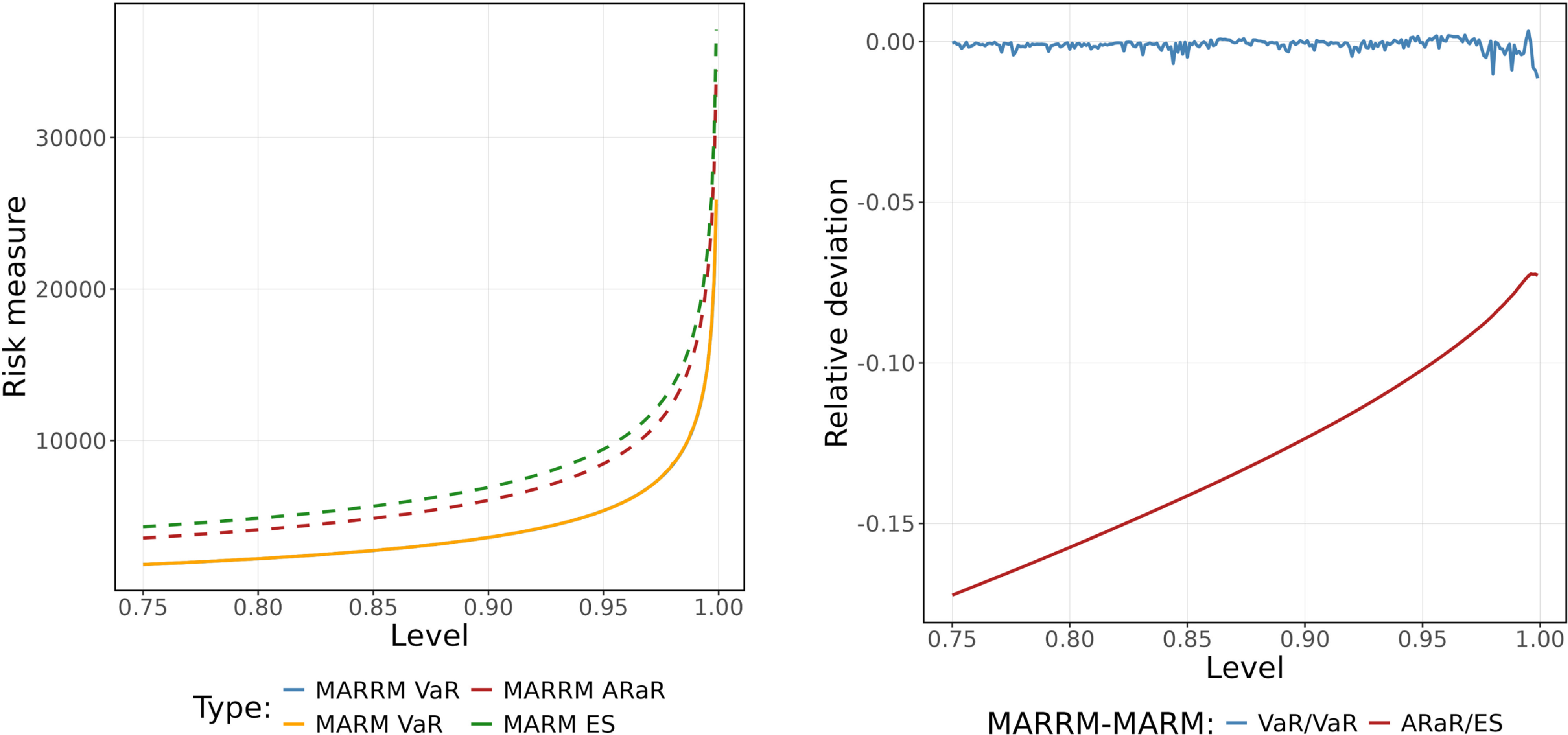
On the left-hand side in Figure 4, we plot the MARRM and MARM for varying levels of the parameter $\lambda$ . Note that the blue and yellow curves overlap. The only curves that are visibly different are the green and the red ones. On the right-hand side, we plot the relative deviation between the two, that is, $\frac{\text{MARRM}-\text{MARM}}{\text{MARM}}$ , as a function of $\lambda$ .

The values in the VaR case differ only minimally, and the difference is solely due to different computational approaches. For MARM, we have to approximate the distribution of $X-Z$ via a Monte-Carlo simulation, while we know the exact value for the MARRM by (3.2). Hence, the difference is fully explained by the Monte-Carlo approximation and the numerical solver used to obtain the minimal hedging price.Footnote ²

The previous point shows that a practitioner can use the MARRM to calculate the MARM in the VaR-case, which has the advantage that a computationally costly Monte-Carlo simulation can be avoided.

The curves in the ES/ARaR-case are not identical. So, in contrast to the VaR-case, a practitioner should be careful in using the MARRM as approximation of the MARM. In Section A.2 of the Online Appendix, we provide additional examples of acceptability criteria where MARRM and MARM differ significantly, with relative differences exceeding 30%.

Figure 4.

LHS: MARM and MARRM risk measures for different levels. RHS: Relative deviation between MARM and MARRM for the same acceptance sets.

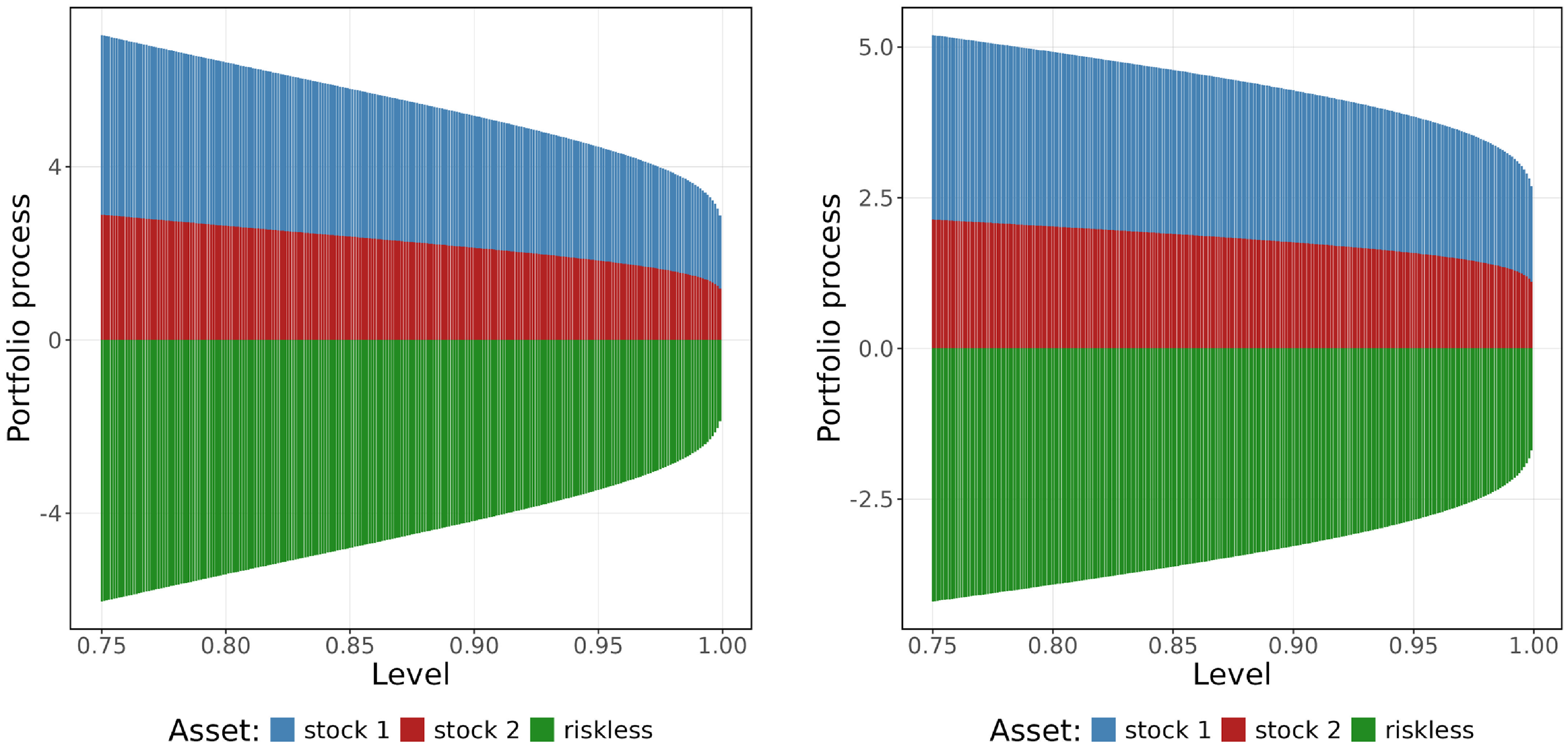
In Figure 5, we return to the topic of risk sharing and the optimal portfolio process for the MARRM depending on the level $\lambda$ for VaR and ARaR. For all levels, the optimal solution admits a short position in the bank account. This short position becomes smaller, if the level increases. We give a detailed explanation of these effects for the VaR-case in Section A.1 of the Online Appendix and show that the large short positions are mainly driven by the log-standard deviation $\sigma=1.0545$ of X. A situation in which smaller values of $\sigma$ occur is the one of logarithmic times series data of financial indices or stocks. In this case, it is possible that no short positions in the bank account occur. For a concrete example, we also refer to the Online Appendix. We can interpret this effect as follows: a larger $\sigma$ results in a heavier tail of the lognormal distribution, which can be more effectively offset by other lognormal distributions than by a constant investment.

Figure 5.

LHS: Optimal portfolio process for MARRM with VaR acceptance set. RHS: Optimal portfolio process for MARRM with ARaR acceptance set.

Finally, we would like to illustrate the risk sharing suggested by the concepts of MARRM and MARM. As mentioned in Section 2.3, the MARRM subdivides the loss X multiplicatively into a security payoff $Z^{x_0,\xi}_T$ and a leverage factor $X/Z^{x_0,\xi}_T$ which lies in the relative acceptance set. Instead, the MARM leads to an additive decomposition of the loss X into a security payoff $Z^{x_0,\xi}_T$ and an acceptable loss $X-Z^{x_0,\xi}_T$ . 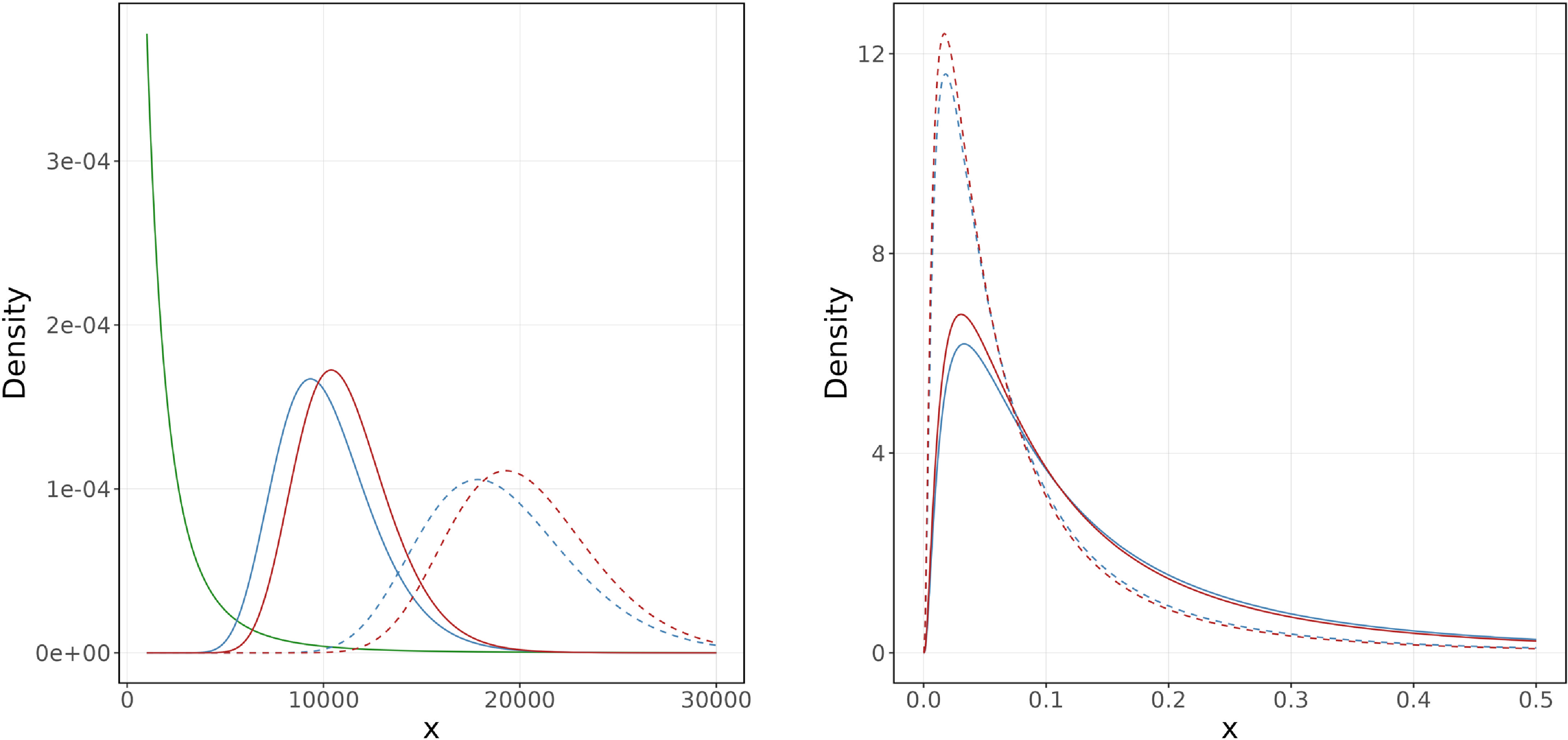In Figure 6, we illustrate on the left-hand side the densities of the loss X and the security payoffs $Z^{x_0,\xi}_T$ for the MARRM and MARM in the ARaR/ES-case at level $\lambda = 0.95$ and $\lambda = 0.99$ . On the right-hand side, we present the densities of the leverage factor for the MARRM. Further, we add the leverage factor densities by using the optimal security payoff calculated via the MARM approach.

The security payoff densities suggest that larger values are more likely under the MARM, explaining why its mode exceeds that of the MARRM density. In multiplicative risk sharing, the leverage factor of the MARM is more likely to produce values near zero, whereas the MARRM places more weight in the tail of the leverage factor.

Figure 6.

In both figures, dashed lines correspond to $\lambda = 0.99$ , solid lines to $\lambda = 0.95$ . LHS: Densities of loss X (green) and the optimal security payoffs for MARRM (blue) and MARM (red). RHS: Densities of the leverage factor $X/Z^{x_0,\xi}_T$ based on the optimal security payoffs in case of the MARRM and MARM.

4.1. Algebraic properties and the reduction lemma

We begin by analyzing under which conditions an MARRM satisfies classical algebraic properties for multi-asset risk measures, namely monotonicity, subadditivity, quasi-convexity, positive homogeneity. In particular, as for classical monetary risk measures or multi-asset risk measures more generally, it turns out that quasi-convexity is equivalent to convexity; see Theorem 4.3. Further, we state some preliminary results that we need later.

For the first result, we recall that a set $\mathcal{A}\subset L^{0}_{++}$ is a cone if $\lambda \mathcal{A}\subset \mathcal{A}$ holds for each $\lambda\in(0,\infty)$ . It is star-shaped if the inclusion $\lambda\mathcal{A}\subset\mathcal{A}$ holds for all $\lambda\in(0,1)$ . Note that we do not require that zero is an element of the set in our definitions of a cone and a star-shaped set, because the sets we are working with are typically subsets of $L^0_{++}$ . Furthermore, given $\mathcal A\subset L^0$ , a map $f\colon\mathcal{A}\rightarrow({-}\infty,\infty]$ is positively homogeneous, if $\mathcal{A}$ is a cone and for each $\lambda\in(0,\infty)$ and $X\in\mathcal{A}$ we have that $f(\lambda X)=\lambda f(X)$ . The map f is star-shaped, if $\mathcal{A}$ is star-shaped and for all $\lambda\in(0,1)$ and $X\in\mathcal{A}$ it holds that $f(\lambda X)\leq \lambda f(X)$ .

The proof of Lemma 4.1 is straightforward and shall be omitted.

In the following lemma, we use the notation $\mathcal{S}_m\;:\!=\{Z\in\mathcal{S}\,;\,\pi(Z)=m\}$ for all $m\gt0$ . We call it “reduction lemma” as it is the counterpart of the result in (Farkas et al. Reference Farkas, Koch-Medina and Munari2015, Lemma 3).

Lemma 4.2. If $\mathcal{S}$ is a cone and $\pi$ is positively homogeneous, then

\begin{align*} \eta_{\mathfrak{R}}(X) &= \inf\left\{\lambda \gt0\,;\,\tfrac{X}{\lambda}\in\mathcal{B}\cdot \mathcal{S}_1\right\}. \end{align*}

Further, the set $\mathcal{B}\cdot \mathcal{S}_1$ is monotone in the following sense:

$$ \forall\,X\in\mathcal{B}\cdot \mathcal{S}_1\,\,\forall\,Y\in \mathcal{C}:\quad Y\leq X\quad\implies\quad Y\in\mathcal{B}\cdot \mathcal{S}_1.$$

Proof. We only prove the second statement. Let $B\in\mathcal{B},Z\in\mathcal{S}_1,Y\in \mathcal{C}$ with $Y\leq B Z$ . Then, $\frac{Y}{Z}\in\mathcal{B}$ , which implies that $Y\in\mathcal{B}\cdot \mathcal{S}_1$ .

For classical risk measures, quasi-convexity describes that the risk measure does not punish, but rather rewards diversification; see, for example, Cerreia-Vioglio et al. (Reference Cerreia-Vioglio, Maccheroni, Marinacci and Montrucchio2011), El Karoui and Ravanelli (Reference El Karoui and Ravanelli2009). Moreover, cash-additivity of monetary risk measures guarantees that quasi-convexity is equivalent to convexity. For MARRMs, we have to substitute cash-additivity by positive homogeneity to obtain such an equivalence. This is the implication “ $(ii)\Rightarrow(iii)$ ” in the next result, which relies on the following fact: A quasi-convex and positively homogeneous map with range $[0,\infty]$ is subadditive. This statement fails for classical risk measures because their range is the extended real line. In addition, the next result shows that convexity for MARRMs is characterized by the set $\mathcal{B}\cdot \mathcal{S}_1$ from the reduction lemma.

Proof. Applying Lemma 4.2 and using that $\mathcal{C}$ is a cone, it holds for all $X\in \mathcal{C}$ that

\[\eta_{\mathfrak{R}}(X) = \inf\left\{\lambda \gt0\,;\,\tfrac{X}{\lambda}\in(\mathcal{B}\cdot \mathcal{S}_1)\cap \mathcal{C}\right\}.\]

“ $(i)\Rightarrow(ii)$ ”: Let $X,Y\in \mathcal{C}$ and choose an arbitrary $\alpha\in(0,1)$ . Without loss of generality, we assume that $\eta_{\mathfrak{R}}(X)\leq \eta_{\mathfrak{R}}(Y)$ . By the monotonicity of $\mathcal{B}\cdot \mathcal{S}_1$ and $\mathcal{C}$ being a cone, we obtain for all $\lambda_X\in(\eta_{\mathfrak{R}}(X),\infty)$ and for all $\lambda_Y\in(\eta_{\mathfrak{R}}(Y),\infty)$ that $\tfrac{X}{\lambda_X}\in(\mathcal{B}\cdot \mathcal{S}_1)\cap \mathcal{C}$ and $\tfrac{Y}{\lambda_Y}\in(\mathcal{B}\cdot \mathcal{S}_1)\cap\mathcal{C}$ . So, by the convexity of $(\mathcal{B}\cdot \mathcal{S}_1)\cap\mathcal{C}$ , we get for all $\lambda \in(\eta_{\mathfrak{R}}(Y),\infty)$ that

\begin{align*} \alpha \tfrac{X}{\lambda} + (1-\alpha) \tfrac{Y}{\lambda} \in (\mathcal{B}\cdot \mathcal{S}_1)\cap \mathcal{C}. \end{align*}

This shows that for $\lambda \in(\eta_{\mathfrak{R}}(Y),\infty)$ , the condition $\frac{Y}{\lambda}\in(\mathcal{B}\cdot \mathcal{S}_1)\cap \mathcal{C}$ implies that $\alpha \frac{X}{\lambda} + (1-\alpha) \frac{Y}{\lambda} \in (\mathcal{B}\cdot \mathcal{S}_1)\cap \mathcal{C}$ . Hence, $\eta_{\mathfrak{R}}(\alpha X + (1-\alpha) Y)\leq \eta_{\mathfrak{R}}(Y)$ .

“ $(ii)\Rightarrow(iii)$ ”: Pick a pair $X,Y\in\mathcal C$ such that $\eta_{\mathfrak{R}}(X)\lt\infty$ and $\eta_{\mathfrak{R}}(Y)\lt\infty$ . If this condition is not satisfied, the defining inequality for subadditivity is automatically satisfied. Let $\varepsilon\gt0$ be arbitrary and set $\lambda_X(\varepsilon)\;:\!=\eta_{\mathfrak{R}}(X)+\varepsilon$ , $\lambda_Y(\varepsilon)\;:\!=\eta_{\mathfrak{R}}(Y)+\varepsilon$ , and $\alpha\;:\!=\lambda_X(\varepsilon)/(\lambda_X(\varepsilon)+\lambda_Y(\varepsilon))$ . By (ii), we know that $\eta_{\mathfrak{R}}$ is quasi-convex, which gives us that

\begin{align*} \eta_{\mathfrak{R}}\left(\tfrac{X+Y}{\lambda_X(\varepsilon)+\lambda_Y(\varepsilon)}\right)&=\eta_{\mathfrak{R}}\left(\alpha \tfrac{X}{\lambda_X(\varepsilon)} + (1-\alpha)\tfrac{Y}{\lambda_Y(\varepsilon)}\right)\leq \max\left\{\eta_{\mathfrak{R}}\left(\tfrac{X}{\lambda_X(\varepsilon)}\right), \eta_{\mathfrak{R}}\left(\tfrac{Y}{\lambda_Y(\varepsilon)}\right)\right\}. \end{align*}

Further, by Lemma 4.1 (ii), $\eta_{\mathfrak{R}}$ is positively homogeneous, which gives us that

\begin{align*} \eta_{\mathfrak{R}}(X+Y)\leq\max\left\{\tfrac{\lambda_X(\varepsilon)+\lambda_Y(\varepsilon)}{\lambda_X(\varepsilon)}\eta_{\mathfrak{R}}(X), \tfrac{\lambda_X(\varepsilon)+\lambda_Y(\varepsilon)}{\lambda_Y(\varepsilon)}\eta_{\mathfrak{R}}(Y)\right\}. \end{align*}

Letting $\varepsilon\downarrow 0$ , we get the desired inequality.

“ $(iii)\Rightarrow(iv)$ ”: $\eta_{\mathfrak{R}}$ being positively homogeneous and subadditive implies that $\eta_{\mathfrak{R}}$ is convex.

“ $(iv)\Rightarrow(i)$ ”: We perform a proof by contraposition. To do so, note that $(\mathcal{B}\cdot \mathcal{S}_1)\cap \mathcal{C}$ not being convex and $\mathcal{C}$ being convex implies that there exist $X,Y\in(\mathcal{B}\cdot \mathcal{S}_1)\cap \mathcal{C}$ and $\alpha\in(0,1)$ such that $\alpha X + (1-\alpha) Y \in \mathcal{C}\backslash (\mathcal{B}\cdot \mathcal{S}_1)$ . Finally, by the monotonicity of $\mathcal{B}\cdot \mathcal{S}_1$ , we obtain

$$ \alpha\eta_{\mathfrak{R}}(X)+(1-\alpha)\eta_{\mathfrak{R}}(Y) \leq 1 \lt \eta_{\mathfrak{R}}(\alpha X + (1-\alpha) Y).$$

In the following example, we elaborate further on the condition of $(\mathcal{B}\cdot \mathcal{S}_1)\cap \mathcal{C}$ being convex. We illustrate that, even if $\mathcal B$ , $\mathcal S_1$ , and $\mathcal C$ are convex, this intersection may or may not be convex.

Example 4.4. Let $\Omega = \{\omega_1,\omega_2\}$ , that is, we can identify $L^{0}$ with the two-dimensional plane $\mathbb{R}^{2}$ . Further, we set $\mathcal{C}=(0,\infty)\times(0,\infty)$ and assume that

$$ \mathcal{S} = \{\lambda (1,1)^{\intercal}+\mu(0.1,2)^{\intercal}\,;\,\lambda,\mu\in(0,\infty)\}.$$

Suppose that the pricing map $\pi$ is linear and given by $\pi((1,1)^{\intercal})=\pi((0.1,2)^{\intercal})=1$ . Hence,

$$ \mathcal{S}_1= \{\lambda (1,1)^{\intercal}+(1-\lambda)(0.1,2)^{\intercal}\,;\,\lambda\in[0,1]\}.$$

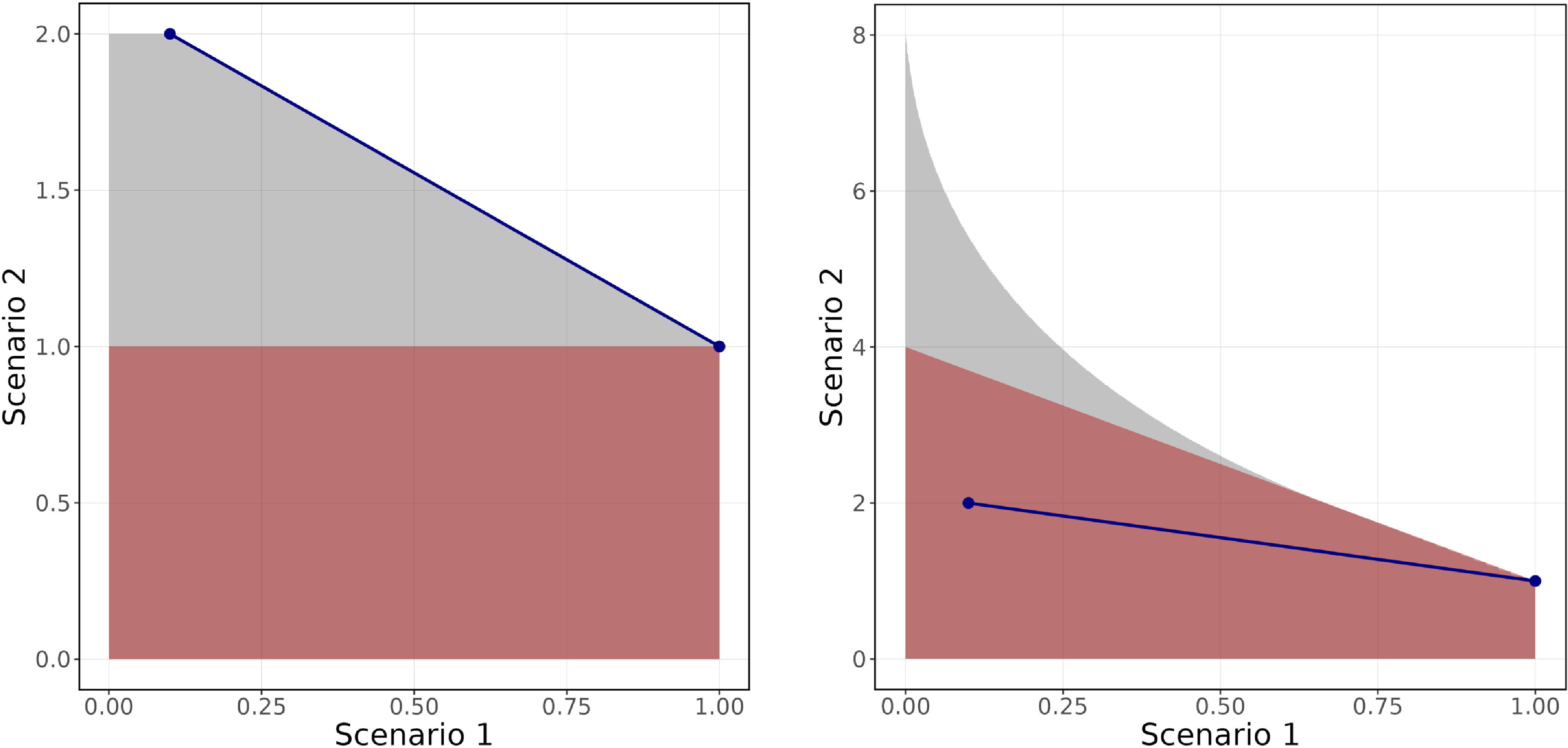
Figure 7 contains the “worst-case relative acceptance set” $\mathcal{B}_{\text{left}}=\{x\in\mathbb{R}^2\,;\,x_1\leq 1, x_2\leq 1\}$ on the left-hand and $\mathcal{B}_{\text{right}}=\{x\in\mathbb{R}^2\,;\,x_1\leq 1,\,x_2\leq 4-3x_1\}$ on the right-hand side. We can see that $(\mathcal{B}_{\text{left}}\cdot \mathcal{S}_1)\cap \mathcal{C}=\mathcal{B}_{\text{left}}\cdot \mathcal{S}_1$ is convex, while $\mathcal{B}_{\text{right}}\cdot \mathcal{S}_1$ fails to be convex.

Figure 7.

In both figures, the red surface represents the relative acceptance set $\mathcal{B}$ , while the blue line is the set $\mathcal{S}_1$ of security payoffs with price 1. The gray and red surface together is the set $\mathcal{B}\cdot\mathcal{S}_1$ . LHS: The set $\mathcal{B}\cdot\mathcal{S}_1$ is convex. RHS: The set $\mathcal{B}\cdot\mathcal{S}_1$ is not convex.

Remark 4.5. Note, $\mathcal{B}\cdot \mathcal{S}_1$ being convex is a stronger condition than $(\mathcal{B}\cdot \mathcal{S}_1)\cap \mathcal{C}$ being convex. To obtain a convex set $\mathcal{B}\cdot \mathcal{S}_1$ , it is intuitive (but not necessary) to choose a relative acceptance set $\mathcal{B}$ which is convex. However, a typical form of such a relative acceptance set is given by

$$ \mathcal{B} = \{X\in\mathcal{C}\,;\,\nu(\log(X))\leq 0\}$$

with a monetary risk measure $\nu$ . In this situation, convexity of $\mathcal{B}$ is equivalent to convexity of $\nu\circ\log$ . Example 4.6 below shows that this condition can be violated, even if $\rho $ is convex. Such a discussion is missing for (Bellini et al. Reference Bellini, Laeven and Rosazza Gianin2018, Lemma 1 (b)).

Example 4.6. Suppose that the underlying probability space is atomless. Select an event $A\in\mathcal F$ and a probability level p with $0\lt P(A)\lt p\lt\frac 1 2$ , and set $x\;:\!=1-\frac{P(A)}{1-p}$ . Moreover, for a constant $a\gt0$ , we consider $X=e^{a} 1_A + 1_{A^c}$ and $Y=1_{A}+e^{a} 1_{A^c}$ .

The Expected Shortfall at level p for $Z\in L^1$ is defined by $\textrm{ES}_{p}(Z) = \frac{1}{1-p}\int_{p}^{1}q_{Z}^{-}(u)\textrm{d}u$ . With this definition, we obtain

\[ \lambda \textrm{ES}_{p}(\log(X)) + (1-\lambda) \textrm{ES}_{p}(\log(Y))= a \left(1-\lambda x\right)=\!:\;f_1(\lambda, x, a). \]

Note that $\lambda X + (1-\lambda) Y = (\lambda e^{a} + (1-\lambda))1_A + ((1-\lambda) e^{a} + \lambda) 1_{A^c}$ . Then, for $\lambda \gt \frac{1}{2}$ , we obtain

\begin{align*} \textrm{ES}_{p}(\log(\lambda X + (1-\lambda) Y) = (1-x)\log(\lambda e^a + (1-\lambda)) + x \log((1-\lambda) e^{a} + \lambda) =\!:\; f_2(\lambda, x, a). \end{align*}

Then, $f_2(0.75,0.5,100) \gt 99.1 \gt 62.5 = f_1(0.75,0.5,100)$ shows that $\textrm{ES}_{p} \circ \log$ is not convex.

Now, we state a sufficient condition to obtain a property that we call “log-star-shapedness” of the MARRM. By Remark 4.8 below, this property holds, if the relative acceptance set is defined via a star-shaped monetary risk measure. Star-shaped monetary risk measures have recently been studied in detail in Castagnoli et al. (Reference Castagnoli, Cattelan, Maccheroni, Tebaldi and Wang2022), Laeven et al. (Reference Laeven, Rosazza Gianin and Zullino2023a, Reference Laeven, Rosazza Gianin and Zullino2023b).

For the next result, given a constant $\alpha\gt0$ and a set $\mathcal{A}\subset{L^{0}}$ , we use the notation $\mathcal{A}^{\alpha}$ for the set of powers $\{X^{\alpha}\,;\,X\in\mathcal{A}\}$ . We call a set $\mathcal{A}\subset L^0_{++}$ log-star-shaped, if for all $\alpha\in(0,1)$ it holds that $\mathcal{A}^{\alpha}\subset\mathcal{A}$ . For such a set $\mathcal{A}$ , we call a map $f:\mathcal{A}\mapsto[0,\infty]$ log-star-shaped, if for all $\alpha\in(0,1)$ and $X\in\mathcal{A}$ it holds that $f(X^{\alpha})\leq f(X)^{\alpha}$ .

Proof. Note that for a subset $\mathcal{A}\subset L^0_{++}$ and for all $\alpha\in(0,1)$ it holds that $\mathcal{A}^{\alpha}\subset\mathcal{A}$ if and only if $\mathcal{A}\subset\mathcal{A}^{\frac{1}{\alpha}}$ . Then, for an arbitrary $\alpha\in(0,1)$ , we obtain

\begin{align*} \eta_{\mathfrak{R}}(X^{\alpha}) &= \inf\left\{\pi(Z)\,;\,Z\in\mathcal{S},\tfrac{X^{\alpha}}{Z}\in\mathcal{B}\right\}= \inf\left\{\pi\left(W^{\alpha}\right)\,;\,W\in\mathcal{S}^{\frac{1}{\alpha}},\,\tfrac{X^\alpha}{W^\alpha}\in\mathcal{B}\right\}\\ &\leq \inf\left\{\pi(W)^{\alpha}\,;\,W\in\mathcal{S}^{\frac{1}{\alpha}},\,\tfrac{X^\alpha}{W^\alpha}\in\mathcal{B}\right\}\\ &\leq \inf\left\{\pi(W^\alpha)\,;\,W\in\mathcal{S},\,\tfrac{X^\alpha}{W^\alpha}\in\mathcal{B}\right\}\leq \inf\left\{\pi(W)^{\alpha}\,;\,W\in\mathcal{S},\,\tfrac{X^\alpha}{W^\alpha}\in\mathcal{B}\right\}\\ &= \inf\left\{\pi(W)^{\alpha}\,;\,W\in\mathcal{S},\tfrac{X}{W}\in\mathcal{B}^{\frac{1}{\alpha}}\right\}\leq \inf\left\{\pi(W)^{\alpha}\,;\,W\in\mathcal{S},\tfrac{X}{W}\in\mathcal{B}\right\}\\ &= \eta_{\mathfrak{R}}(X)^{\alpha}. \end{align*}

Remark 4.8. The assumption of $\mathcal C$ being log-star-shaped is satisfied if $\mathcal C=L^p_{++}$ with $p\in[1,\infty]\cup\{0\}$ .

In Section 2.2, we mention relative acceptance sets of the form

\begin{align*} \mathcal B=\{X\in\mathcal{C}\,;\,\nu(\log(X))\le 0\} \end{align*}

with $\nu$ being a monetary risk measure. If $\nu$ is star-shaped, then $\mathcal{B}$ is log-star-shaped. Specifying $\nu$ as Value-at-Risk or Expected Shortfall delivers the relative acceptance sets used, for example, in the empirical study in Section 3 or in McNeil and Frey (Reference McNeil and Frey2000).

The assumption of $\mathcal S$ being log-star-shaped is satisfied if $\mathcal{S}$ models all possible positive payoffs in a complete continuous-time financial market model. It is also satisfied in the situation of Section 3, where we use a Black–Scholes model with trading opportunities restricted to constant portfolio processes. Additionally, $\mathcal S$ being log-star-shaped also holds for the Wishart volatility market in Bäuerle and Li (Reference Bäuerle and Li2013), which admits the famous Heston model as special case.

Finally, if the pricing functional is given by a (worst-case) expectation with respect to a (family of) pricing density, then the property of $\pi$ holds due to Jensen’s inequality.

As argued in (Laeven and Rosazza Gianin Reference Laeven and Rosazza Gianin2022, Section 3), natural properties of RRMs rewarding diversification in a context of continuously rebalanced portfolios are logconvexity and quasi-logconvexity. Continuous portfolio rebalancing means the proportion of wealth invested in each asset remains constant, while total wealth may vary over time. This requires reallocating wealth across available assets over time, in contrast to buy-and-hold strategies, which are more straightforward in conjunction with monetary risk measures. The following proposition collects sufficient conditions to obtain (quasi-)logconvexity for MARRMs.

Proposition 4.9. Assume that each set $\mathcal D\in\{\mathcal{C},\mathcal{B},\mathcal{S}\}$ is logconvex, that is,

$$ X,Y\in\mathcal D\text{ and }\alpha\in(0,1)\quad\implies\quad X^\alpha Y^{1-\alpha}\in\mathcal D.$$

1. (i) Suppose that $\pi$ is quasi-logconvex, that is,

   $$ \pi(X^\alpha Y^{1-\alpha})\le\max\{\pi(X),\pi(Y)\},\quad X,Y\in\mathcal C,\,\alpha\in(0,1).$$
   Then, $\eta_{\mathfrak{R}}$ is also quasi-logconvex.

2. (ii) Suppose that $\pi$ is logconvex, that is,

   $$ \pi(X^\alpha Y^{1-\alpha})\le\pi(X)^{\alpha}\pi(Y)^{1-\alpha},\quad X,Y\in\mathcal C,\,\alpha\in(0,1).$$
   Then, $\eta_{\mathfrak{R}}$ is also logconvex.

Proof. The proof is analogous to the corresponding one of Proposition 4.7.

4.2. Finiteness and relative acceptability arbitrage

Now, we discuss situations in which the MARRM does not attain $\infty$ . In particular, this is the case in the studies (Bellini et al., Reference Bellini, Laeven and Rosazza Gianin2018; Laeven and Rosazza Gianin, Reference Laeven and Rosazza Gianin2022).

Lemma 4.10. Let ${\mathfrak{R}}$ be a return risk measurement regime. Then $\eta_{\mathfrak{R}}$ is finite-valued if and only if

$$ \mathcal C\subset\mathcal S\cdot\mathcal B.$$

If $\mathcal{C}= L^{\infty}_{++}$ , then the latter condition is satisfied if $\mathcal S$ contains all positive multiples of an element in $\textrm{int}(L^\infty_{+}) = \{X\in L^{\infty}\,;\,\exists\,\varepsilon\gt0\colon X\geq \varepsilon\text{ a.s.}\}$ and $1\in\mathcal{B}$ .

Proof. Clearly, $\eta_{\mathfrak{R}}(X)\lt\infty$ if and only if one can find $Z\in\mathcal S$ and $Y\in\mathcal B$ such that $X=Z\cdot Y$ . Now assume that $\mathcal C=L^\infty_{++}$ and assume that $X\in\mathcal C$ is arbitrary. For suitable $U\in \textrm{int}(L^\infty_{+})$ and $\lambda\gt0$ , we have that $X\leq \lambda U$ . By monotonicity of $\mathcal{B}$ and $1\in\mathcal{B}$ , $\tfrac{X}{\lambda U}\in\mathcal{B}$ . As $\lambda U\in\mathcal S$ by assumption, this means $\eta_{\mathfrak{R}}(X)\le \pi(\lambda U)\lt\infty$ .

The condition $\mathcal{C}\subset \mathcal{S}\cdot\mathcal{B}$ means that any loss in $\mathcal{C}$ can be made relatively acceptable by buying an appropriate market portfolio in $\mathcal{S}$ .

If $\eta_{\mathfrak{R}}(X)=0$ , then there exists a sequence $\{Z_n\}\subset \mathcal{S}$ satisfying $\lim_{n\to\infty}\pi(Z_n)=0$ such that $\frac{X}{Z_n}\in \mathcal{B}$ holds for all $n\in\mathbb{N}$ . This means that market wealth relative to which the position X is acceptable is available in the market at arbitrarily small initial investment. Hedging at arbitrarily small cost is known in the context of classical risk measures, as “acceptable arbitrage” opportunity, see for example, Artzner et al. (Reference Artzner, Delbaen and Koch-Medina2009). This suggests that we call an X with $\eta_{\mathfrak{R}}(X)=0$ a “relative acceptability arbitrage” opportunity. The next goal is to find conditions to avoid relative acceptability arbitrage opportunities. We start this discussion with the situation of positions in $L^{\infty}$ .

Proof. By $\mathcal{B}$ being a nonempty proper subset of $\mathcal{K}$ , there exists $Y\in\mathcal{K}\backslash\mathcal{B}$ . By $X\in\textrm{int}(L^{\infty}_+)$ , we know that there exists $\varepsilon\gt0$ such that $X\geq \varepsilon$ almost surely. Since Y is bounded from above, we can find $0\lt\lambda^*\lt\varepsilon$ such that for all $0\lt\lambda \lt \lambda^*$ it holds that $\frac{X}{\lambda}\geq \frac{\varepsilon}{\lambda}\geq Y\notin\mathcal{B}$ . This shows that $\eta_{\mathfrak{R}}(X)\geq \lambda^*\gt0$ .

The next example shows that $X\notin\textrm{int}(L^{\infty}_+)$ can lead to $\eta_{\mathfrak{R}}(X)=0$ .

Example 4.12. Assume that the underlying probability space is atomless and consider the following relative acceptance set:

\begin{align*} \mathcal{B} = \{Y\in L^{\infty}_{++}\,;\, P(Y\leq 1)\gt0\}. \end{align*}

It is easy to check that $\mathcal B$ is monotone, that $1\in\mathcal{B}$ , and that $2\notin\mathcal{B}$ . Now, if X is distributed uniformly over (0,1) then for all $m\in(0,1)$ we have $P\left(\frac{X}{m}\leq 1\right)\gt0$ , and hence $\frac{X}{m}\in\mathcal{B}$ . For $\mathcal{S} = (0,\infty)$ this implies that $\eta_{\mathfrak{R}}(X)=0$ .

The previous example shows that even in the case of $\mathcal{C}=L^{\infty}_{++}$ we need additional assumptions on $\mathcal{S}$ , $\pi,$ and $\mathcal{B}$ to obtain $\eta_{\mathcal{R}}\gt0$ . We suggest a combination of two assumptions which are sufficient to guarantee positivity of $\eta_{\mathfrak{R}}$ . The first, Assumption 4.13, is motivated by the no free lunch with vanishing risk (NFLVR) condition and concerns the financial market given by $\pi$ and $\mathcal{S}$ . The second, Assumption 4.14, is our conclusion from Example 4.12 and concerns only the preferences of an agent given by $\mathcal{B}$ . The advantage is that these are separate assumptions for the financial market and the preferences of an agent. Hence, we do not artificially link them in a single assumption.

Assumption 4.13. For each sequence $\{Z_n\}\subset \mathcal{S}$ with $\pi(Z_n)\to 0$ , $n\to\infty$ , we have

$$ P(0\lt Z_n)\rightarrow 0,\quad n\to\infty.$$

Proof. Towards a contradiction, assume that there exists $X\in\mathcal{C}$ such that $\eta_{\mathfrak{R}}(X) = 0$ . Then, there exists a sequence $\{Z_n\}\subset \mathcal{S}$ with $\pi(Z_n)\rightarrow 0$ and $\frac{X}{Z_n}\in\mathcal{B}$ for all n.

By the nontriviality of $\mathcal{B}$ , there exists $Y\in\mathcal{K}\backslash\mathcal{B}$ . Further, by Assumption 4.13, we obtain

\begin{align*} P\big(\tfrac{X}{Z_n}\gt Y\big) = 1 - P\big(\tfrac{X}{Z_n}\leq Y\big) = 1 - P\big(\tfrac{X}{Y}\leq Z_n\big)\rightarrow 1. \end{align*}

Hence, by Assumption 4.14, we obtain that $\frac{X}{Z_n}\notin \mathcal{B}$ for all but finitely many n, a contradiction.

4.3. Properties regarding MARRMs and MARMs

In order to be precise, we work until the rest of the manuscript in the setting of Proposition 2.13. Our aim is to point out which properties of MARMs and MARRMs are equivalent to each other (see Lemma 4.18). To do so, we have to characterize properties of the model ingredients (see Lemma 4.17). We omit the direct proofs of the next two results.

We can use this setting to generalize Lemma 2 (b), (d)–(f) in Bellini et al. (Reference Bellini, Laeven and Rosazza Gianin2018).

Quasi-logconvexity in point (b) in Lemma 4.18 describes the reward for diversification for continuously rebalanced portfolios. In this case, a payoff admits the following form: $Y = \exp(\omega_A r_A + \omega_B r_B)$ , where $r_A$ and $r_B$ are the log-returns of two investment opportunities A and B and $\omega_A$ and $\omega_B$ are the portfolio weights, that is, the percentage of capital invested in one of the investment opportunities. The latter implies that $\omega_A+\omega_B = 1$ . So, if $\omega_A\in(0,1)$ , then we have diversified our portfolio. Quasi-logconvexity of $\eta_{\mathfrak{R}}$ then gives us that $\eta_{\mathfrak{R}}(Y)\leq\max\{\eta_{\mathfrak{R}}(\exp(r_A)),\eta_{\mathfrak{R}}(\exp(r_B))\}$ . Hence, quasi-convexity describes that the MARRM rewards diversification of relative amounts. Especially, in Section 3 in Laeven and Rosazza Gianin (Reference Laeven and Rosazza Gianin2022), the authors conclude that quasi-convexity for classical risk measures is related to buy-and-hold strategies, whereas quasi-logconvexity is related to rebalanced portfolios.

A similar interpretation holds for submultiplicative MARRMs. For this, Assumption 2.9 ensures that the product of two random variables $X,Y\in\mathcal{C}$ is still an element of $\mathcal{C}$ . Note, the product of two losses corresponds to a squared amount of money. This is consistent with the upper bound, which is also a squared amount of money as a product of two MARRMs.

5.1. Assumption on $\mathcal{C}_{\log}$

Our approach is similar to the one in Aygün et al. (Reference Aygün, Bellini and Laeven2024). The first step is to choose $\mathcal{C}_{\log}$ , while the set $\mathcal{C}$ is obtained as a consequence and not controlled directly. This is also motivated by practitioners working with time-series models commonly using log-returns as input for the risk measure $\rho_{\mathcal{A}_{\nu},\mathcal{S}_{\log},\pi_{\log}}$ . Hence, log-returns are the objects of interest, and it is therefore natural to start by choosing the set $\mathcal{C}_{\log}$ .

Our aim is to leverage the representation of an MARRM via an MARM and the existence of a dual representation of the latter to obtain a dual representation of the MARRM in question. To do so and to perform convex duality arguments, we equip $\mathcal{C}_{\log}$ with a topology $\tau_{\log}$ and make the following standing assumption:

This assumption means that we choose a topology on $\mathcal{C}_{\log}$ and not on $\mathcal{C}$ directly. The following example contains the two most common choices for $\mathcal{C}_{\log}$ in this situation.

5.2. Dual representations

For the next proof, we denote the topological dual space of a locally convex space $\mathcal{X}$ by $\mathcal{X}^{\prime}$ . Further, a real-valued function $\varphi$ on a suitable set $\mathcal{C}\subset L^0_{++}$ is called log-linear, if $\varphi\left(X^{\alpha}Y^{\beta}\right) = \alpha\varphi(X)+\beta\varphi(Y)$ for all $X,Y\in\mathcal{C}$ and $\alpha,\beta\in\mathbb{R}$ , assuming tacitly that such products lie in $\mathcal C$ . For instance, if $\psi\colon \mathcal{C}_{\log} \to\mathbb{R}$ is linear, then $\psi\circ\log$ is a log-linear functional on $\mathcal C$ . Conversely, in the upcoming proofs, we set

$$ \varphi_{\log}(Y)=\varphi(e^Y),\quad Y\in\mathcal C_{\log}.$$

By log-linearity of $\varphi$ , for all $\alpha\in\mathbb{R}$ and $Y,Y'\in\mathcal C_{\log}$ ,

$$ \varphi_{\log}(Y+\alpha Y')=\varphi(e^Y(e^{Y'})^\alpha)=\varphi(e^Y)+\alpha\varphi(e^{Y'})=\varphi_{\log}(Y)+\alpha\varphi_{\log}(Y').$$

Hence, each log-linear and $\tau$ -continuous map $\varphi$ can be transformed by $\varphi\circ \exp$ into a linear and $\tau_{\log}$ -continuous map.

For the remainder of this section, we use the notation from Section 2.2, that is, $\tilde{\rho}\colon\mathcal{C}\rightarrow (0,\infty)$ is an RRM, $\nu=\log\circ\tilde{\rho}\circ \exp$ , $\mathcal{A}_{\nu}=\{X_{\log}\in\mathcal{K}_{\log}\,;\,\nu(X_{\log})\leq 0\}$ and $\pi_{\log}=\log\circ\pi\circ \exp$ is defined on $\mathcal S_{\log}$ .

We start with a dual representation for a logconvex MARRM.

Proposition 5.4. Suppose that $\rho_{\mathcal{A}_{\nu},\mathcal{S}_{\log},\pi_{\log}}$ is proper, convex, and lower semicontinuous with respect to $\tau_{\log}$ . Consider the associated return risk measurement regime ${\mathfrak{R}}=(\mathcal B_{\tilde\rho},\mathcal S,\pi).$ Then, for all $X\in\mathcal C$ , the MARRM $\eta_{\mathfrak{R}}$ can be represented as

(5.1) \begin{align} \eta_{\mathfrak{R}}(X) = \sup_{\varphi\in\mathcal{D}_{\geq 1}}\exp\left(\varphi(X)-\left(\sup_{Y\in\mathcal{B}_{\tilde{\rho}}}\varphi(Y)\right)-\left(\sup_{Z\in\mathcal{S}}\varphi(Z)-(\log\circ\pi)(Z)\right)\right), \end{align}

where $\mathcal{D}_{\geq 1} = \{\varphi\colon\mathcal{C}\rightarrow\mathbb{R}\,;\, \varphi\text{ log-linear}, \tau\text{-continuous}, \forall X\in\mathcal{C}\cap\mathcal{K}\text{ with }X\geq 1\colon\varphi(X)\geq 0\}.$

Proof. Working with a locally convex space $(\mathcal{C}_{\log},\tau_{\log})$ (Assumption 5.1) and by the assumption that $\rho_{\mathcal{A}_{\nu},\mathcal{S}_{\log},\pi_{\log}}$ is proper, convex, and lower semicontinuous, we are allowed to apply the well-known Fenchel–Moreau Theorem. Then, following the reasoning of the proof of Proposition 3.9 in Frittelli and Scandolo (Reference Frittelli and Scandolo2006), we obtain for $X_{\log}\in\mathcal{C}_{\log}$ that

\begin{align*} \rho_{\mathcal{A}_{\nu},\mathcal{S}_{\log},\pi_{\log}}(X_{\log}) = \sup_{\psi\in(\mathcal{C}_{\log})^{\prime}}\Big(\psi(X_{\log})-\Big(\sup_{Y_{\log}\in\mathcal{A}_{\nu}}\psi(Y_{\log})\Big)-\Big(\sup_{Z_{\log}\in\mathcal{S}_{\log}}\psi(Z_{\log})-\pi_{\log}(Z_{\log})\Big)\Big). \end{align*}

By the fact that $\mathcal{A}_{\nu}-(\mathcal{K}_{\log})_{+}\subset\mathcal{A}_{\nu}$ , we can restrict the dual representation to functionals $\psi\in(\mathcal{C}_{\log})^{\prime}$ such that for all $X_{\log}\in(\mathcal{C}_{\log}\cap\mathcal{K}_{\log})_{+}$ it holds that $\psi(X_{\log})\geq 0$ . By a reformulation in terms of the model ingredients of the MARRM, we obtain the desired representation.

Now, we use two weaker assumptions than being logconvex. First, we assume that the MARRM is log-star-shaped as defined in the context of Proposition 4.7. Second, we assume that the MARRM is quasi-logconvex; see Proposition 4.9.

We start with log-star-shapedness. To the best of our knowledge, it is the first time that a dual representation for this type of functionals is mentioned in the literature.

Theorem 5.6. Let $\rho_{\mathcal{A}_{\nu},\mathcal{S}_{\log},\pi_{\log}}$ be proper, star-shaped, and normalized, that is, $\rho_{\mathcal{A}_{\nu},\mathcal{S}_{\log},\pi_{\log}}(0) = 0$ . Then the dual representation of the MARRM is given for $X\in\mathcal{C}$ by

(5.2) \begin{equation} \eta_{\mathfrak{R}}(X) = \min_{W\in\textrm{dom}\left(\eta_{\mathfrak{R}}\right)}\sup_{\varphi\in\mathcal{D}}\exp\Bigg(\varphi(X) -\sup_{\substack{Z\in\mathcal{S}\\ Y\in\mathcal{B}_{\tilde{\rho}}\\ W = YZ}}\max\left\{0,\varphi(Y)+\varphi(Z)-(\log\circ\pi)(Z)\right\}\Bigg), \end{equation}

where $\mathcal{D} = \{\varphi\;:\;\mathcal{C}\rightarrow\mathbb{R}\,;\, \varphi\text{ log-linear}, \tau\text{-continuous}\}=\{\varphi_{\log}\circ\log\,;\,\varphi_{\log}\in\mathcal (C_{\log})'\}$ .

Proof. $(\mathcal{C}_{\log},\tau_{\log})$ being a locally convex space (Assumption 5.1) and $\rho_{\mathcal{A}_{\nu},\mathcal{S}_{\log},\pi_{\log}}$ is proper, star-shaped, and normalized meaning that all assumptions to apply Proposition 8 in Laeven et al. (2023a) are satisfied. By this result, we obtain for $X_{\log}\in\mathcal{C}_{\log}$ that

(5.3) \begin{align} \rho_{\mathcal{A}_{\nu},\mathcal{S}_{\log},\pi_{\log}}(X_{\log}) = \min_{W_{\log}\in\textrm{dom}\left( \rho_{\mathcal{A}_{\nu},\mathcal{S}_{\log},\pi_{\log}}\right)}\sup_{\psi\in(\mathcal{C}_{\log})^{\prime}}\left(\psi\left(X_{\log}\right)-f^{*}_{W_{\log}}(\psi)\right), \end{align}

where $f^{*}_{W_{\log}}$ is the convex conjugate of the following function:

\begin{align*} f_{W_{\log}}(X_{\log}) = \begin{cases} \alpha\rho_{\mathcal{A}_{\nu},\mathcal{S}_{\log},\pi_{\log}}(W_{\log}), &\exists\alpha\in[0,1]\;:\; X_{\log} = \alpha W_{\log},\\ +\infty, &\text{otherwise}. \end{cases} \end{align*}

For the convex conjugate of $f_{W_{\log}}$ , we obtain

\begin{align*} f^{*}_{W_{\log}}(\psi)&= \sup_{X_{\log}\in\mathcal{C}_{\log}}\left(\psi\left(X_{\log}\right)-f_{W_{\log}}(X_{\log})\right)= \sup_{\alpha\in[0,1]}\alpha\left(\psi\left(W_{\log}\right)-\rho_{\mathcal{A}_{\nu},\mathcal{S}_{\log},\pi_{\log}}(W_{\log})\right)\\ &= \sup_{\alpha\in[0,1]}\sup_{\substack{Z_{\log}\in\mathcal{S}_{\log}\\ W_{\log}-Z_{\log}\in\mathcal{A}_{\nu}}}\alpha\left(\psi\left(W_{\log}\right)-\pi_{\log}(Z_{\log})\right)\\ &= \sup_{\substack{Z_{\log}\in\mathcal{S}_{\log}\\ Y_{\log}\in\mathcal{A}_{\nu} \\ W_{\log} = Y_{\log}+Z_{\log}}}\max\{0,\psi\left(Y_{\log}\right)+\psi\left(Z_{\log}\right)-\pi_{\log}(Z_{\log})\}. \end{align*}

Using this in combination with (5.3) and an analogous reformulation in terms of the model ingredients of the MARRM as it is done in the proof of Proposition 5.4 gives us the result.

Now, we analyze the case of a quasi-logconvex MARRM. As in Laeven and Rosazza Gianin (Reference Laeven and Rosazza Gianin2022), our result is based on the dual representation of quasi-convex functions in (Volle Reference Volle1998, Theorem 3.4). For a more compact version of this result, we refer to (Frittelli and Maggis Reference Frittelli and Maggis2011, Theorem 1.1).

Theorem 5.8. Assume that $\rho_{\mathcal{A}_{\nu},\mathcal{S}_{\log},\pi_{\log}}$ is quasi-convex and lower semicontinuous. Then, the dual representation of the MARRM is given for $X\in\mathcal{C}$ by

(5.4) \begin{align} \eta_{\mathfrak{R}}(X) =\sup_{\varphi\in\mathcal{D}}\inf\{\pi(Z)\,;\,Z\in\mathcal{S}, W\in\mathcal{B}_{\tilde{\rho}}, \varphi(W)\geq \varphi(X)-\varphi(Z)\}, \end{align}

with $\mathcal{D}$ as in Proposition 5.4.

Proof. By applying Theorem 3.4 in Volle (Reference Volle1998), which holds because $(\mathcal{C}_{\log},\tau_{\log})$ is locally convex (Assumption 5.1) and $\rho_{\mathcal{A}_{\nu},\mathcal{S}_{\log},\pi_{\log}}$ is quasi-convex and lower semicontinuous, we obtain for $X_{\log}\in\mathcal{C}_{\log}$ that

(5.5) \begin{align} \rho_{\mathcal{A}_{\nu},\mathcal{S}_{\log},\pi_{\log}}(X_{\log}) = \sup_{\psi\in(\mathcal{C}_{\log})^{\prime}}\sup\Bigg\{r\in\mathbb{R}\,;\,\psi(X_{\log})\gt \sup_{\substack{Y_{\log}\in\mathcal{C}_{\log}\\ \rho_{\mathcal{A}_{\nu},\mathcal{S}_{\log},\pi_{\log}}(Y_{\log})\lt r}}\psi(Y_{\log})\Bigg\}. \end{align}

As it is pointed out in Theorem 1.1 in Frittelli and Maggis (Reference Frittelli and Maggis2011), it can be shown that Equation (5.5) is equal to

\begin{align*} \rho_{\mathcal{A}_{\nu},\mathcal{S}_{\log},\pi_{\log}}(X_{\log}) = \sup_{\psi\in(\mathcal{C}_{\log})^{\prime}}\inf_{\substack{Y_{\log}\in\mathcal{C}_{\log}\\ \psi(Y_{\log})\geq \psi(X_{\log})}}\rho_{\mathcal{A}_{\nu},\mathcal{S}_{\log},\pi_{\log}}(Y_{\log}). \end{align*}

Using the definition of the MARM, we obtain:

\begin{align*} \rho_{\mathcal{A}_{\nu},\mathcal{S}_{\log},\pi_{\log}}(X_{\log}) &= \sup_{\psi\in(\mathcal{C}_{\log})^{\prime}}\inf_{\substack{Y_{\log}\in\mathcal{C}_{\log}\\ \psi(Y_{\log})\geq \psi(X_{\log})}}\inf_{Z_{\log}\in\mathcal{S}_{\log}}\Big(\pi_{\log}(Z_{\log})+\delta_{\mathcal{A}_{\nu}}(Y_{\log}-Z_{\log})\Big)\\ &= \sup_{\psi\in(\mathcal{C}_{\log})^{\prime}}\inf_{Z_{\log}\in\mathcal{S}_{\log}}\inf_{\substack{W_{\log}\in\mathcal{A}_{\nu}\\ \psi(W_{\log})\geq \psi(X_{\log})-\psi(Z_{\log})}}\pi_{\log}(Z_{\log}). \end{align*}

A reformulation in terms of the ingredients of the MARRM gives us (5.4).

Remark 5.9. For $\varphi\in\mathcal{D}$ set $\sigma_{\mathcal{B}_{\tilde{\rho}}}(\varphi)=\sup_{Y\in\mathcal{B}_{\tilde{\rho}}}\varphi(Y)$ . If the supremum is attained, then we can write

\begin{align*} \inf\{\pi(Z)\,;\,Z\in\mathcal{S}, W\in\mathcal{B}_{\tilde{\rho}},\varphi(W)\geq \varphi(X)-\varphi(Z)\}=\inf\{\pi(Z)\,;\,\sigma_{\mathcal B_{\tilde\rho}}(\varphi)\geq \varphi(X)-\varphi(Z)\}. \end{align*}

We use this to compare Proposition 5.4 and Theorem 5.8: The representation (5.4) leads to the model $\varphi$ for which the minimum hedging costs $\pi(Z)$ are maximized subject to the existence of an acceptable loss with larger logarithmic costs (under $\varphi$ ) than the ones for $\frac{X}{Z}$ . In particular, the objective is only the price $\pi(Z)$ of a market portfolio Z.

If the MARRM satisfies the stronger condition of log-convexity, then representation (5.1) holds. Here, for a model $\varphi$ , we do not restrict the set of hedging payoffs by the inequality $0\geq \varphi(X)-\varphi(Z)-\sigma_{\mathcal{B}_{\tilde{\rho}}}(\varphi)$ . Instead, $\varphi(X)-\varphi(Z)-\sigma_{\mathcal{B}_{\tilde{\rho}}}(\varphi)$ appears in the objective directly (as a penalty term). This means, a model $\varphi$ for which the logarithmic costs $\varphi(X)-\varphi(Z)$ are larger than the ones for an acceptable loss (under $\varphi$ ) leads to a penalization of $(\log\circ\pi)(Z)$ .

In summary, log-star-shapedness prevents separation of the market components $\mathcal{S}$ , $\pi$ , and the relative acceptance set $\mathcal{B}_{\tilde{\rho}}$ in the dual representation (5.2) and leads to a penalty for possible models $\varphi$ without rewards, due to the additional maximization with zero in (5.2).

For the dual representation (5.4) of quasi-logconvex MARRMs, we obtain that only hedging costs are used as objective function and terms which occur as summands in the dual representation (5.1) of logconvex MARRMs only occur in a constraint.

5.3. Duality without Assumption 5.1

In this section, we discuss the impact of Assumption 5.1. Typical choices for $\mathcal{C}$ are different to the ones by working under Assumption 5.1. For instance, think of an RRM $\tilde\rho\colon L^\infty_{++}\to(0,\infty)$ as defined in Definition 2.6. As recalled above, $\nu\colon \mathcal{C_{\log}}\to\mathbb{R}$ with $\mathcal{C}_{\log}=\{Y\in L^0\,;\, \exists\,c\in\mathbb{R}\colon Y\leq c \text{ a.s.}\}$ defined by $\nu(Y)=(\log\circ\tilde\rho\circ \exp)(Y)$ . But, $\mathcal{C}_{\log}$ is only a convex cone and not a linear space. Hence, Assumption 5.1 does not hold. By the fact that $L^{\infty}\subset \mathcal{C}_{\log}$ , the representations from the previous section only hold for the restricted function $\tilde{\rho}|_{\textrm{int}(L^{\infty}_{+})}$ .

The previous example shows that a dual representation for an MARM on $L^\infty$ gives us a representation for the corresponding MARRM with domain $L^{\infty}_{++}$ restricted to $\textrm{int}(L^{\infty}_{+})$ . Analogously, a dual representation for an MARM on $L^p$ with $p\in[1,\infty)$ gives us a representation for the corresponding MARRM with domain $L^p_{++}$ restricted to the set $\{X\in L_{++}^{p}\,;\,\log(X)\in L^p\}$ .

So, it is an open question how to obtain a dual representation if we start with $\mathcal{C}$ instead of $\mathcal{C}_{\log}$ . If the MARRM is not only logconvex but also convex, one idea is to apply convex duality directly to the MARRM and avoid the usage of the connection with MARMs. The main difficulty is that in the situation of $\mathcal{C}\subset L^1$ , $\mathcal{C}$ is not a closed convex cone in a suitable $L^p$ -norm topology. This means, even if the MARRM $\eta_{\mathfrak{R}}$ is lower semicontinuous on $\mathcal{C}$ , then it is not clear under which assumptions we can extend $\eta_{\mathfrak{R}}$ to a lower semicontinuous function on the norm-closure of $\mathcal{C}$ .

We only demonstrate an example in which the latter is possible and for completeness, we also state the dual representation stemming from Proposition 5.4.

Example 5.10. Assume the RRM is given by the $L^1$ -norm $\tilde{\rho}\colon L^1_{++}\ni X\mapsto \mathbb{E}[X]$ . We can extend this functional to all of $L^1$ by

\begin{align*} f\colon L^{1}\rightarrow [0,\infty],\quad X\mapsto\begin{cases} \mathbb{E}[X], &X\in L^{1}_{+},\\ \infty, &X\notin L^{1}_{+}. \end{cases} \end{align*}

In this case, f is proper, convex, and lower semicontinuous. Hence, by the Fenchel–Moreau Theorem it holds that the Fenchel–Legendre biconjugate $f^{\ast\ast}$ of f is equal to f itself. This delivers for all $X\in L^{1}_{++}$ the dual representation

(5.6) \begin{align} \tilde{\rho}(X) = f(X) = \sup\big\{\mathbb{E}[YX]\,;\,Y\in L^{\infty},\left\lVert Y\right\lVert_{\infty}\leq 1\big\}=\mathbb{E}[X]. \end{align}

Alternatively, we can apply Proposition 5.4 to obtain for all $X\in \{W\in L^{1}_{++}\,;\, \log(W)\in L^1\}$ that

(5.7) \begin{align} \tilde{\rho}(X) = \sup\big\{\exp\big(\mathbb{E}[Y\log(X)]-H(Y|P)\big)\,;\,Y\in L_{+}^{\infty},E[Y]=1\big\}, \end{align}

where $H(Y|P) =\mathbb{E}[Y\log(Y)]$ is the relative entropy of Y with respect to P. Thus, the results from the previous subsection only gives us a dual representation for elements of a specific subset. Further, (5.7) is a representation based on the behavior of the log-return of X. Hence, the representation admits a geometrical behavior, due to the exponential function in this formula. Note, the relative entropy occurs due to the fact that $\log\circ\tilde{\rho}\circ \exp$ is the entropic risk measure. In contrast, (5.6) is obtained by directly applying the Fenchel–Moreau Theorem to $\tilde{\rho}$ . Hence, the log-return of X does not play a role here.