At the start of the twentieth century, labor productivity in German manufacturing was about half the level of its American counterpart. During the subsequent period, until the outbreak of WWII, this gap did not narrow. If anything, productivity in German manufacturing fell even further behind (Broadberry Reference Broadberry1997). Traditional explanations for Europe's inability to catch-up give prominence to differences in technology driven by local circumstances, in particular factor and resource endowments. Compared to Europe, the United States was well endowed with natural resources, while skilled labor was relatively expensive, resulting in a more capital-intensive production process. Furthermore, American demand for goods was more homogenous and given the size of the domestic market, U.S. manufacturers could standardize production and implement high throughput systems, providing abundant opportunity for capital intensification and resource use. Divergent development paths across the Atlantic emerged: an American mass production system dependent on relatively unskilled workers using special purpose machinery versus European flexible production methods based on skilled labor using general purpose machines. With different technological trajectories, labor-productivity gaps remained (Rothbarth Reference Rothbarth1946; Habakkuk Reference Habakkuk1962; Temin Reference Temin1971; David Reference David1975; Field Reference Field1985; Broadberry Reference Broadberry1994).
However, some of the elements in this explicative model for the U.S./German productivity gap have recently been called into question. Case studies suggest that technology gaps between Germany and the United States declined as new technologies were transferred across the Atlantic already during the early twentieth century. In her study on German modernization, Mary Nolan (Reference Nolan1994) notes that American influences on German entrepreneurship were limited before WWI. But “(w)ith the end of Germany's acute postwar dependency and instability, America came to be seen as an economic model. In the words of one observer: ‘One seeks to learn from her, to study her organization, management, and technology’” (Nolan Reference Nolan1994, p. 38). Many German entrepreneurs traveled to the United States to study first-hand the organization of American manufacturing industries and deployed imitating activities to catch up with their American competitors (Braun Reference Braun and Smith1984). Alfred Chandler (Reference Chandler1992) observes that on average German firms conform more closely to the American model of business organization than British firms. Contemporary industry periodicals report a variety of cases where German manufacturers imported American machinery and incorporated these in domestic production lines (Richter and Streb Reference Richter and Streb2011). Apart from a new coat of paint, this was often installed in its original form. A particular striking example is the German machine-tool industry (Ristuccia and Tooze Reference Ristuccia and Tooze2013). By the late 1930s the number of advanced machines per worker installed on the factory floor was comparable between the United States and Germany. Arguably, this boasted other manufacturing industries that made extensive use of domestically produced machine tools, leading to a further diffusion of modern production techniques. This evidence does not fit easily in a model of dichotomous technological paths across the Atlantic (Richter Reference Richter2008). It begs the question whether the Germans ought to be seen as “the Yankees of Europe” instead, a term used by Robert Lowie in his portrait of the German people (quoted by Kindleberger Reference Kindleberger1978, p. 188).
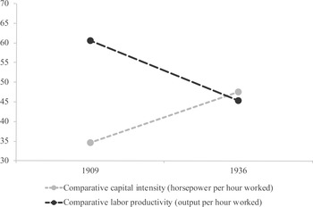
In this article we will outline a new explanatory framework that accommodates the seemingly contradictory pieces of evidence on German productivity and technology trends. We start with quantifying the paradox. How fast exactly were transatlantic differences in the use of production techniques disappearing and how persistent was the labor-productivity gap? We first discuss trends in installed horsepower in German and U.S. manufacturing industries, which we argue to be the relevant proxy for the choice of production techniques. It is shown that during 1909–1936 in most German manufacturing industries growth in horsepower per hour worked was higher than in the United States, even in industries such as chemicals and machinery, which might be surprising given the dynamism of these industries in the United States (Field Reference Field2003). In a second step we provide a new U.S./German comparison of labor productivity (real value added per hour worked) for manufacturing industries for 1936 using detailed information from the first complete industrial census for Germany (Fremdling, de Jong, and Timmer Reference Fremdling, de Jong and Timmer2007). Combining these new pieces of evidence in Figure 1, a clear puzzle emerges: while labor productivity in German manufacturing fell further behind U.S. levels during 1909–1936, the capital-intensity gap narrowed.
COMPARATIVE LABOR PRODUCTIVITY AND CAPITAL INTENSITY IN MANUFACTURING, U.S. = 100

To explain this puzzle, we develop a new empirical framework to decompose cross-country differences in labor productivity into differences in the use of production techniques (measured as horsepower per hour) on the one hand, and differences in the efficiency with which techniques are used on the other. This is different from traditional analyses grounded in the Solow (Reference Solow1956) model, either in a time-series perspective, known as growth accounting, or in a cross-country setting, known as level accounting. Labor-productivity differences are accounted for by differences in capital per worker and a residual, known as total factor productivity (TFP). However, it is well known that this approach suffers from major shortcomings (Abramovitz Reference Abramovitz1956; Broadberry Reference Broadberry1997). Most important from the perspective of our study is its inability to account for inefficiency. Typically, differences in TFP are interpreted as differences in disembodied technology, but this only holds under the assumption that all countries are efficient, that is, they are using factor inputs to their full potential. It is a well-established fact, however, that there are many barriers to full efficiency, and that these will differ across countries and over time (Arrow Reference Arrow1962; Habakkuk Reference Habakkuk1962; David Reference David1975; Chandler Reference Chandler1990; Rosenberg Reference Rosenberg1994). In particular, in circumstances of rapid innovation, the introduction and assimilation of new techniques will be inefficient as firms need time to learn to operate machinery at its full potential. As stressed by Kenneth Arrow (Reference Arrow1962, p. 155) in his study of the economic implications of learning by doing: “Learning is the product of experience…. Learning can only take place through the attempt to solve a problem and therefore only takes place during activity.” This learning process might be particularly strong during the interwar period, which witnessed rapid technological change and innovation (Field Reference Field2003) and generated many inefficiencies in technology use.
To measure inefficiency in the use of techniques we follow Subodh Kumar and Robert Russell (Reference Kumar and Russell2002) by applying Data Envelopment Analysis (DEA). This methodology constructs a global best-practice frontier that indicates for each given technique the highest output per worker that potentially can be attained. The difference between the actual labor productivity level in a country and the potential level indicates the inefficiency with which the technique is operated. Cross-country differences in labor productivity at a particular point in time will thus be decomposed into differences in technique (installed horsepower per hour worked) and differences in efficiency with which the technique is used, as measured by the distance to the frontier. The functional form of the frontier is not chosen in advance, but empirically determined as the envelope over a large set of real-world observations of output and input combinations. Importantly, by putting only minimal restrictions on the shape of the global frontier, it can reflect different speeds of technological change at various levels of capital intensity. This allows us to empirically capture the idea of different technological trajectories and localized innovation as emphasized by Anthony Atkinson and Joseph Stiglitz (Reference Atkinson and Stiglitz1969).
The original Kumar and Russell (Reference Kumar and Russell2002) approach was developed for decomposing productivity growth rates and we extend it in two ways. We are the first to apply this method to decompose cross-country productivity gaps. Our approach thus improves upon the level accounting exercises as applied by, for example, Stephen Broadberry (Reference Broadberry1997) in a similar way as Kumar and Russell (Reference Kumar and Russell2002) improved upon traditional growth accounting. Secondly, we increase the method's relevance for historical analysis by modelling the frontier at time t as the global pool of technologies used at t, as well as in the period before such that there is no “forgetting” (Los and Timmer Reference Los and Timmer2005). This historical approach is particularly relevant for our case as we will compare countries that might differ in the timing of technology adoption: a technique introduced in say the United States might only diffuse later in another country. To determine the global frontier, we constructed a novel database of value added, labor and machinery input in German, British, and American industries for the period 1899–1936, including new measures of industry purchasing power parities (PPPs) to convert cross-country outputs into a common currency.
With method and data at hand, we will show that the lack of German catch-up in labor productivity in innovative industries such as machinery, electrical engineering, andchemicals is due mainly to the inefficiency with which advanced techniques were used, rather than to differences in production techniques. These inefficiencies arose as American methods of production needed to be adapted to local circumstances. The latter have been pointed to before as a determinant of labor-productivity levels (e.g., Chandler Reference Chandler1990; Rosenberg Reference Rosenberg1994; Broadberry Reference Broadberry1994, Reference Broadberry1997). The crucial novelty here, however, is that local circumstances suppressed labor productivity not so much by discouraging the adoption of modern production techniques, but more by constraining the efficient use thereof. We will call this the “inefficient assimilation” explanation. In contrast, for less dynamic industries such as textiles and metals production, the traditional “dichotomous technology path” explanation still seems to hold as lagging German productivity levels resulted predominantly from following a different technological trajectory indicated by wide gaps in capital intensity. Our findings are suggestive of a more refined model of transatlantic productivity differences that accounts for differences across industries, and puts localized innovation, technological learning as well as barriers to technology assimilation center stage.
GERMAN CATCH UP IN CAPITAL INTENSITIES, 1909–1936
In this section we introduce installed horsepower per hour worked as our preferred measure of capital intensity. We discuss its strengths and weaknesses, as well as available data sources. Results show that, in many industries, German manufacturing was catching up with the United States during the interwar period, fitting the observations from more qualitative studies.
Installed Horsepower as a Proxy for Capital Intensity
To determine transatlantic gaps in capital intensity, we propose a comparison of the amount of installed horsepower per hour worked. Much of the production knowledge gained since the Second Industrial Revolution was contained in tangible capital in the form of machinery installed on the factory floor (Broadberry Reference Broadberry1997, p. 108). Information on machine investment and stocks is not abundant, however, and hard to compare across countries. While data on investment in equipment is available from the historical national accounts (Kendrick Reference Kendrick1961; Hoffmann Reference Hoffmann1965; Feinstein Reference Feinstein1972), they do not provide the level of detail needed for an in-depth analysis at the industry level. There is some scattered information on capital stock overall, but machinery has historically been a relatively small proportion of the capital stock, which has been dominated by structures and buildings (Field Reference Field1985). Therefore, we proxy the value of machines by installed horsepower, following Harry Jerome (Reference Jerome1934), Broadberry and Rainer Fremdling (Reference Broadberry1990), Herman de Jong (Reference de Jong2003), and Nicholas Crafts (Reference Crafts2004). An advantage of this approach is that the statistics are abundantly available and readily comparable over time and across countries as they are in physical units, not requiring time series of investments, deflators, and depreciation as for capital stock measures.
We will make a comparison of horsepower installed per hour worked in Germany and the United States for 1909 and 1936, a period which captures the major technological changes in the early twentieth century (Field Reference Field2003). To match the latter year as closely as possible we use the 1935 U.S. census. Hence throughout the article the comparisons are made for Germany in 1936 with the United States in 1935. For brevity we will refer to this as “1936” comparisons, unless stated otherwise. Horsepower and employment statistics can be found directly in the German national employment censuses and the U.S national production censuses. More details on data sources can be found in Appendix 1 and in the Online Supporting Material.
The horsepower proxy of capital intensity is not without problems, however, and two particular worries need to be addressed. A first concern relates to so-called “double counting.” The horsepower applied on the factory floor is supplied by machinery running on either non-electric or electric power. In case of the latter, the electricity needed to operate the machinery can be internally generated in the factory (by electricity generators) or purchased from an electrical power network to which the factory is connected. When the electricity is internally generated, the horsepower used by electricity generators should be excluded in the analysis as it does not contribute directly to the fabrication of goods. We correct the horsepower figures for the effect of double counting.Footnote 1
Second, there is an unstable relation between operated horsepower and the machine stock during our period of study. This is related to the electrification of the production process in general and the introduction of the electric unit drive in particular. With electric unit drive, which became widespread since the 1920s, each machine tool is directly connected to its own electric power supply and no longer reliant on a single line shaft or group drive. This new set-up allowed for greater flexibility and enhanced production efficiency, while at the same time increasing the total power capacity of installed machinery (Schurr et al. Reference Schurr, Burwell and Devine1990). Warren Devine (Reference Devine1983, p. 362) observes that “with unit drive, each motor had to be of sufficient capacity to handle the maximum demand of its machine; with group drive, the motor could be sized to take advantage of load diversity, i.e., only the average load of a group (plus a safety margin) needed to be met because each machine in the group operated only part of the time.” This is problematic when the rate of electrification differed across the Atlantic. However, as shown in the Online Supporting Material, electrification rates in German and U.S. manufacturing were much the same, both in the pre-WWI and interwar period, which indicates that they adopted electric power systems at a similar speed. The share of electric in total horsepower in overall manufacturing increased from 20 to 76 percent in Germany (1907–1933), while from 22 to 82 percent in the United States (1909–1929), with similar developments at more detailed industries (see Online Supporting Material).
German Catch-up to U.S. Capital Intensity Levels
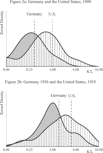
Based on the horsepower statistics we find that in general German manufacturing was catching up with the United States during the interwar period. This is captured by Figure 2. Two Kernel-density plots are drawn, each of which displays the distribution of manufacturing employment over available capital-intensity levels (K/L) in Germany and the United States based on observations for 73 industries. In 1909, German manufacturing produced at much lower capital-labor ratios than the United States (Figure 2a). However, the overlap of the U.S. and German distributions in the late 1930s demonstrates that capital-intensity levels in Germany were catching up to the United States (Figure 2b). At the aggregate manufacturing level, the level in Germany increased from 35 percent of the United States in 1909 to 48 percent in 1936. Note that in the United States horsepower per hour more than tripled over the period. But even though the United States had invested heavily in new technology, particularly during the 1920s (Field Reference Field2003), Germany had been able to increase its capital-intensity level faster. Moreover, at the rate of change between 1909 and 1936, Germany would have achieved the U.S. capital-intensity level of 1935 by the late 1940s. The sizable share of small firms in German manufacturing makes the rapidity of this catch-up process all the more remarkable (Kinghorn and Nye Reference Kinghorn and Nye1996; Hannah Reference Hannah2008). Smaller firms tend to lack the necessary financial resources to invest in new technology, but still the average gap in capital-intensity levels to the United States decreased.
DISTRIBUTION OF MANUFACTURING EMPLOYMENT OVER MACHINE-INTENSITY LEVELS

This finding fits the observations from more qualitative case studies of German industries (e.g., Berthold Reference Berthold1988). Joachim Radkau (Reference Radkau1989) observes that as early as between 1870 and 1914 German manufacturers acquired machinery in the United States, yet the practice of technology adoption was limited to large and advanced German establishments, mostly in metal-producing and metal-processing industries. In this first wave, the American technologies were met with doubts concerning their applicability in Germany and implementation was frequently deemed feasible only once machinery was modified to suit local conditions. The second wave of Americanization took place in the 1920s and was much more widespread. Smaller firms participated in imitating activities too, as it was recognized that copying U.S. production technology improved competitiveness and reduced development costs (Richter Reference Richter2008). American production technology became the prime vision of modernity among German industrialists. Many German entrepreneurs traveled to the United States to study first-hand the organization of U.S. manufacturing industries. Despite the differences in conditions, it was argued that the principles of American production technology could be isolated and implemented in Germany as well (Nolan Reference Nolan1994; Braun Reference Braun and Smith1984).
In the Online Supporting Material, we provide more detailed results at the two- and three-digit industry levels. It shows that Germany followed developments in the United States in many industries, albeit at different distances which suggests that a one-size-fits all explanation of transatlantic productivity gaps must be reconsidered. For example, in cotton and rayon manufactures, the gap in horsepower intensity actually increased. In contrast, the gap declined considerably in chemical manufacturing. In this industry, horsepower intensities increased by almost five times in the United States, but even more in Germany such that the gap had shrunk from one-third of the U.S. level in 1909 to halve the U.S. level in 1936. In sub-industries such as gum and wood chemicals German horsepower intensity levels were even higher than in the United States. Another prominent example of Germany leading in capital intensity is provided by the metal working and industrial machinery industry. This fits the findings of more detailed studies. Ralf Richter and Jochen Streb (Reference Richter and Streb2011) quote contemporary sources reporting that American machine tools were copied by German engineers without any modification to the original design.Footnote 2 Richter (Reference Richter2008) concludes that not only thousands of American machine tools were in use in Germany, but also the same amount or even more German copies of these tools. In a more recent article, Cristiano Ristuccia and Adam Tooze (Reference Ristuccia and Tooze2013) analyze the number of purchased machines in Germany and the United States and found clear convergence such that by the 1930s both countries operated very similar machine-worker ratios. Moreover, they find that German additions to the machinery stock consisted of new technologies not unlike those in America. On the basis of this evidence, they reject the notion of dichotomous technological paths across the Atlantic, at least in this industry.
In light of this evidence, it is difficult to maintain for the early twentieth century the notion that Germany was stuck on a technology path very different from the United States. Various German industries showed catch-up in capital-intensity levels during 1909–1936, even in new industries that featured high levels of technological change. However, in 1936 labor-productivity levels in Germany were still much lower than in the United States. How much can be accounted for by the remaining gaps in capital-intensity, and how much is explained by the inefficient use of the new capital? To answer this question, we need to use a decomposition analysis that allows for the measurement of efficiency in the use of inputs.
LABOR PRODUCTIVITY DECOMPOSITION FRAMEWORK
In this section we will outline our framework for decomposing the labor-productivity gap between Germany and the United States into two elements: a gap in capital intensity and a gap in the efficiency with which capital is being used. To do so we built upon the empirical model of a global productivity frontier introduced by Kumar and Russell (Reference Kumar and Russell2002). We extend this model in two ways. First, we will apply this method to decompose cross-country productivity gaps, rather than productivity growth in a particular country as in their original analysis. Second, we increase the method's relevance for historical analysis by modelling the global frontier not only on the contemporaneous set of observations, but also observations on inputs and outputs in the period before. This reflects the idea that knowledge of production technologies may spill over not only across countries, but also over time.
Basic Decomposition of Labor Productivity Gaps
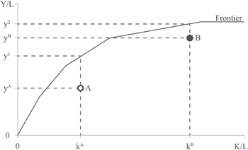
For the decomposition of the labor-productivity gap between Germany and the United States, we built upon the empirical model of a global productivity frontier introduced by Kumar and Russell (Reference Kumar and Russell2002). In line with the extant literature we will refer to (differences in) capital intensity also as (differences in) “technique,” and use the term “technology” as a reference to a set of techniques. The basic intuition of the decomposition is illustrated by stylized Figure 3. A German industry (A) and its American counterpart (B) are positioned relative to the global best-practice frontier. This frontier indicates for a given technique the highest output per worker that can be attained, when used fully efficient. It is empirically determined as the envelope over a large set of real-world observations of output and input combinations, as explained below. The observed labor-productivity gap between the two countries (y B /y A ) is attributable, first, to the use of different capital-labor ratios, because the labor-productivity potential (y Footnote 1 and y Footnote 2 ) at the capital-intensity levels of Germany and the United States (k A and k B , respectively) differs. If both countries operate at their respective capital-intensity levels with full efficiency, the United States enjoys a labor-productivity lead over Germany as the American technique has a larger labor-productivity potential. Secondly, the labor-productivity gap is determined by the efficiency level of Germany (y A /y Footnote 1 ) relative to the United States (y B /y Footnote 2 ). If Germany exploits relatively little of its labor-productivity potential compared to the United States, this contributes to the observed labor-productivity gap too.
DECOMPOSITION OF THE LABOR-PRODUCTIVITY GAP

The decomposition is more formally given in equation (1):
![\[
\begin{array}
ln \left (\frac{y^B} {y^A}\right)=ln \left (\frac{y^2} {y^1}\right)+\left[ln\left (\frac{y^B} {y^2}\right)-ln \left (\frac{y^A} {y^1}\right)\right].
\end{array}
\](https://static.cambridge.org/binary/version/id/urn:cambridge.org:id:binary:20170301100616229-0762:S0022050716000760:S0022050716000760_eqn1.gif?pub-status=live)
It shows that if the efficiency component between square brackets on the far right side of equation (1) takes on a value of zero, the productivity gap solely results from the use of different techniques, a scenario much in line with the notion of divergent technology paths across the Atlantic. Alternatively, if capital-intensity levels are close together, then most of the productivity gap is explained by differences in the efficiency with which the techniques are being used. This development we would characterize as “inefficient assimilation.”
Frontier Determination through DEA
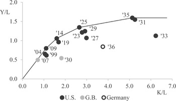
A crucial element in the decomposition framework is the determination of the global technology frontier, which indicates, for a given technique, the maximum labor-productivity level that can be achieved. This maximum is empirically determined based on the productivity performance of a set of countries that also operated this technique, either in the present or in the past. We therefore collected data for the United States, Great Britain, and Germany. Ideally one would like to include more countries, but this is not feasible due to data limitations and arguably these were the most technologically advanced countries of the time. How we determine the global production frontier using DEA is best illustrated by means of Figure 4. In a first step manufacturing industries that produce similar products are sorted into groups on the basis of the U.S. Standard Industrial Classification (henceforth, SIC). Subsequently, for each SIC three-digit industry data on capital intensity as well as labor productivity is collected (see section following for more information on data sources). In Figure 4 a scatter plot example is shown for the chemical fertilizer industry (SIC industry code 287) for 1936. A data point consists of an observation of capital intensity in this industry in a particular country and year (say the United States in 1909), and the realized labor-productivity level (measured as real value added per hour worked). It should be noted that the frontier is estimated using both current and past observations, which is an extension of the original Kumar and Russell (Reference Kumar and Russell2002) model that only considered contemporaneous observations. By including observations from earlier years, we allow for the fact that knowledge previously generated is “remembered” over time and remains accessible in the current period. This increases the relevance for historical analysis as we will be able to compare countries that might differ in the timing of technological adoption: a technique introduced in say the United States might only diffuse later in another country. The earliest data stems from 1899 and we cover a total of 15 years for the period up to and including 1936. The global best-practice frontier is then drawn by enveloping the data in the tightest-fitting convex cone using linear line segments. Thus one can establish for each observation a best-practice benchmark provided by a linear combination of two “peer” observations on the frontier. The distance to the frontier is a measure of the inefficiency with which the technique is operated. For example, the efficiency with which a German technique in 1936 is used is measured by the vertical distance of this observation to a (hypothetical) linear combination of the U.S. observations in 1925 and 1935.
ESTIMATING THE FRONTIER FOR FERTILIZERS IN 1936

The convex enveloping of the data is done by a standard non-parametric linear programming technique, known as DEA. More formally, assume that all inputs and output quantities are non-negative and that at a given time t the production technology set S
t
contains the transformation of N inputs,  , into M outputs,
 :

An input distance function at time t is defined as

Note that, as explained earlier, the production technology set at t includes observations not only from time t, but also includes inputs-to-output transformations realized in previous periods. This reflects the idea that all countries have access to a common global pool of knowledge that is built up over the years. This allows countries to grow by innovating for themselves, or by imitating technologies explored elsewhere in the past. As a side effect, this enlarging of the production technology set also improves the method's statistical robustness, as the number of observations from which the frontier can be determined increases making it less sensitive to measurement error. As we have only three countries in our analysis, this is a highly desirable characteristic.
Suppose there are k observations of realized input-output combinations. Under constant returns-to-scale, the input distance (efficiency index, θ ∗ j ) for a particular observation j is given by the solution to the following linear program (Färe, Grosskopf, and Knox Reference Färe, Grosskopf and Lovell1994):

The θ ∗ j is determined by the distance of j to a (hypothetical) composite producer formed as a nonnegative linear combination of all k observations using weights as given by the vector λ ∗. This composite producer needs no more than θ ∗ j times the inputs of j, while still producing j's output. The efficiency index θ will take on a value between zero and one, where a value of one implies that j is fully efficient. All fully efficient, or “best practice”, observations together determine the position and shape of the production frontier as illustrated in Figure 4.
An appeal of the DEA framework is that the non-parametric nature of this approach puts minimal assumptions of functional form on the frontier, which makes is particularly useful for historical analysis (cf. Färe, Grosskopf, and Knox Reference Färe, Grosskopf and Lovell1994). In contrast to the Solow-model based decompositions it can accommodate the finding that technological change is highly localized as suggested by Atkinson and Stiglitz (Reference Atkinson and Stiglitz1969). Robert Allen (Reference Allen2012) has shown that ever since the First Industrial Revolution innovation mainly took place in techniques characterized by high capital-to-labor ratios. The knowledge generated only spills over to a limited set of similar production techniques. For instance, the innovations introduced in Ford's factory to streamline production at its moving assembly line were not appropriate for production sites that still relied on non-standardized batch production. To reap the benefits of this new knowledge (such as specialized standalone machinery, interchangeable parts, and time-and-motion studies), European car producers had to shift to continuous flow processes instead. The potentially biased nature of technological change will be picked up by the non-parametric determination of the global productivity frontier. As such it is fundamentally different from the traditional Solow-based decomposition frameworks that rely on production functions which shapes are determined by assumptions on relationships of prices and marginal productivity that are questionable, in particular in historical contexts as discussed by Broadberry (Reference Broadberry1997, pp. 105–110). The difference between DEA and the Solow based decomposition is discussed in more depth in Appendix 3.
DECOMPOSITION OF THE 1936 U.S./GERMAN PRODUCTIVITY GAP
In view of our findings on trends in horsepower intensity, it is difficult to maintain the notion that all German industries were stuck on a technology path very different from the United States. At the same time, there is general agreement on the existence of a major productivity gap between Germany and the United State during this period. In his seminal work, Broadberry (Reference Broadberry1997) has already shown that during the early twentieth century German manufacturing productivity levels hovered around British levels, which in turn were about half the U.S. levels. This indirectly implies that German manufacturing performed at roughly half the U.S. level. However, we need to have more detailed industry-level estimates of the labor-productivity gaps that we intend to decompose as we found large heterogeneity in capital-intensity levels across industries. These can only be obtained from a direct comparison, which is possible for 1936, i.e., the year of the first German national census of production. In this section we therefore first present a new benchmark of U.S./German comparative labor productivity for detailed manufacturing industries in 1936. Secondly we present the decomposition of the labor-productivity gap, as established by our new benchmark, in differences in capital intensity and inefficiency using the method previously outlined. The results are highly supportive of a more nuanced understanding of the drivers of the transatlantic productivity gap.
Comparative U.S./German Productivity Levels in 1936
There are two reasons why we need a new direct benchmark of U.S./German comparative labor productivity. The first concern is of a methodological nature. An indirect U.S./German comparison via the United Kingdom is inaccurate because the coverage of industries and products differs between the German/U.K. and U.S./U.K. benchmarks, introducing a potential bias. A second, arguably more important, concern relates to the use of primary sources for Germany. The first official German production census of 1936 is available in two forms: a published edition and the original archival records. The former has been set up to hide manufacturing activities of strategic military importance. The archival records report the original unedited data and are therefore more accurate as well as more extensive. For a comparison between Germany and the United Kingdom, Fremdling, de Jong, and Timmer (Reference Fremdling, de Jong and Timmer2007) showed that the labor-productivity data reported in the published figures—which are used in Broadberry (Reference Broadberry1997)—deviate substantially from the data supplied by the original archival records.
Following Fremdling, de Jong, and Timmer (Reference Fremdling, de Jong and Timmer2007) we use the archival records of the 1936 German census to calculate U.S./German comparative labor productivity. To compare value added across countries a conversion to a common currency is needed. It is well known that the exchange rate is not an optimal conversion factor for this purpose, since—among other things—it only provides information at the total economy level and at best reflects the relative prices of internationally traded goods. We therefore developed a new set of PPPs at the industry level to convert German Reichsmarks to U.S. dollars. These PPPs are based on matching value and quantity information for a set of 202 manufacturing products using the so-called industry-of-origin approach. Product unit value ratios have been derived and aggregated to industry level PPPs. This new set of industry PPPs is presented in the Online Supporting Material. The methodology underlying the industry-of-origin approach is formally described in Appendix 2.
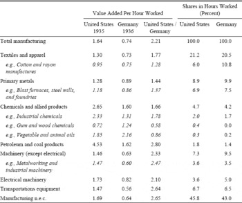
Table 1 reports the new comparison of value added (in U.S. dollar) per hour worked in Germany in 1936 and the United States in 1935. We single out several major industries and sub-industries, which are interesting from a technology perspective and are illustrative of our main story. Full details can be found in the Online Supporting Material. Column three reports the ratio between the American and German productivity levels. Overall, U.S. labor productivity in manufacturing was more than twice the German level. Although the U.S. lead over Germany is somewhat larger than the comparative U.S./German level implied by an indirect comparison based on Broadberry (Reference Broadberry1997), our results corroborate the general view that Germany still lagged far behind the United States before WWII.
LABOR-PRODUCTIVITY COMPARISONS BETWEEN GERMANY (1936) AND THE UNITED STATES (1935)

Notes:
Value added in 1929 US$. More detailed results available from online supporting material.
Sources:
See Appendix 1 for details.
However, there is considerable variation across industries. The comprehensive list of industries in the Online Supporting Material shows a spread of comparative U.S./German levels ranging from 0.58 (gum and wood chemicals) on the low end to 5.12 (watches and clocks) on the high end. In Table 1 we have included the industries with a comparatively strong German performance. Germany was productivity leader only in gum and wood chemicals and vegetable and animal oils. In chemicals and allied products as a whole Germany lagged behind the United States, but at a relatively small distance as compared to other industries. In textiles and primary metals the gap with the United States was small, too. Part of the reason for this may have to do with the fact that these industries produced mainly basic goods. For instance, much of the production in textile industries (yarn and weavings) was used as intermediate input for apparel industries. Similarly, primary metals industries produced basic iron and steel products that were further processed in fabricated metal products and machinery industries. As production was not intended for sale on retail markets and therefore not subject to heterogeneous demand patterns that are often associated with Europe, efficiency gains through standardization of production may have been easier here than in industries producing mainly consumer goods. This notion is strengthened by Germany's weak performance in transportations equipment; particularly in this industry the benefits of standardization (assembly line) were pivotal to labor-productivity gains during the interwar period, but the consumer preferences faced by German producers on domestic markets may have encouraged customized production with limited potential for standardization, an issue we will return to later.
Decomposition of the Labor Productivity Gap
How much of the U.S./German labor-productivity gap can be accounted for by the gaps in capital intensity, and how much is explained by the inefficient use of the new techniques? To answer this question, we use the labor-productivity decomposition given in equation (1). For this, we need three sets of data. First, we require a precise estimate of U.S./German labor-productivity gaps in 1936. The new benchmark presented in Table 1 provides this information. Second, we need a measure of U.S./German capital-intensity gaps in 1936, which were already introduced in Figure 2 and are available in the Online Supporting Material. Third, we need a global technology frontier to indicate the labor-productivity potential for levels of capital intensity. In line with equations (2) to (4), we estimate this frontier on the basis of labor-productivity and capital-intensity data for 1936 and earlier years. We have collected this data from the production censuses of the three industrial leaders of the early twentieth century, i.e., the United States, Great Britain, and Germany, for years between 1899 and 1936. For the U.S. data is collected for the years 1899, 1904, 1909, 1914, 1919, 1923, 1925, 1927, 1929, 1931, 1933, and 1935. For Great Britain data is taken for 1907 and 1930. Germany is included in the dataset in the year 1936. In all, the dataset contains 1,373 observations pairing labor productivity and capital intensity at the three-digit level of the SIC, which aggregates to 357 observations at the SIC two-digit level. A more detailed description of the data sources can be found in Appendix 1. Full details, including the data itself, are available in the Online Supporting Material.
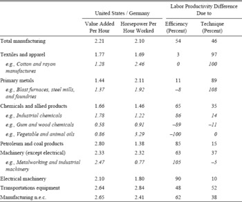
The decomposition results are given in Table 2. The first column provides the labor-productivity gap, repeating from Table 1. The second column gives comparative statistics on the installed horsepower per hour worked, which underlie Figure 2 and provide our measure of capital intensity. For manufacturing as a whole, U.S. levels are slightly more than double the German levels in both productivity and horsepower. The last two columns report the results of the decomposition of the U.S./German labor-productivity gap along the lines of equation (1) into the part accounted for by differences in technique and by differences in the efficiency with which the techniques are used. The last two columns are given in percentages and add up to 100. The table demonstrates that the lower capital-intensity level of Germany accounts for 46 percent of the overall manufacturing productivity gap. With 54 percent, the better part of the gap is due to the lower levels of German efficiency in the use of their techniques. The use of different technique was still important, but it was not the main driver behind the labor-productivity gap.
DECOMPOSITION OF THE 1936 UNITED STATES/GERMANY LABOR-PRODUCTIVITY RATIO

Notes:
Labor productivity decomposition is based on equation (1). More detailed decomposition results available from online Supporting material.
Sources:
See Appendix 1 for details.
Another main finding is the remarkable variation across industries. The results suggest that modern industries in Germany were attempting to imitate and innovate upon frontier techniques developed in the United States, but that, at the same time, efficiency levels for these industries remained relatively low. Table 2 shows that inefficiency explains the major part of the labor-productivity gap in dynamic industry groups like chemicals (65 percent), petroleum (85 percent), machinery (63 percent), and in particular in electrical engineering (90 percent). The table shows that in some subindustries within these major groups lack of efficiency on the part of Germany explains virtually the entire labor-productivity gap. The most notable is metal working and industrial machinery in which installed horsepower in Germany was even higher than in the United States, while labor productivity was substantially lower. Trends in these industries are in line with the case studies discussed in the introduction and our “inefficient assimilation” hypothesis.
In contrast, the productivity gaps in less dynamic industries resulted primarily from differences in technique. For the textiles and apparel, as well as primary metals industries major gaps in capital intensity remained, effectually accounting for all of the labor productivity differences (97 and 89 percent, respectively). Here German manufactures appeared to be operating on a different part of the technology frontier compared to their American competitors, confirming the “dichotomous technology” hypothesis.
Developments in transportation equipment manufacturing do not easily fit into these characterizations. The rate of innovation in this industry was high, but Germany was not able to keep up with developments in the United States. Capital intensity in this industry increased rapidly, though not as fast as in the United States, and major gaps in capital intensity and in labor productivity appeared. In 1936 lower capital intensity accounted for 48 percent of the productivity gap and inefficiency for 52 percent. To account for developments in this industry differences in techniques as well as the inefficient assimilation of techniques need to be considered.
INTERPRETATION
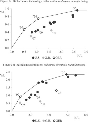
The results of our analysis suggest a more nuanced understanding of industrial development paths in Germany in the early twentieth century. Some industries failed to adopt capital intensities with high productivity potential, conform the traditional notion of dichotomous technology developments across the Atlantic. In this view technical change is incremental and highly path-dependent as countries frugally innovate driven by slowly changing local circumstance and factor prices (David Reference David1975). In contrast, many other industries set out to modernize as innovation in America was so rapid that the new production methods made U.S. technology superior at all relative factor prices. Far from simply copying their American counterparts German firms needed to assimilate the new technologies and adopt it to local settings. These sectors typically operated at low efficiency levels, which accounted for the bulk of the labor-productivity gap. These different development paths are illustrated in Figure 5.
EXAMPLES OF TECHNOLOGY PATHS IN GERMAN INDUSTRIES

Figure 5 shows for two manufacturing industries the developments of Germany in comparative perspective. Each graph contains the estimated global technology frontier for 1936 and also indicates with dots observations for the United States starting in 1899 through 1935, for the United Kingdom in 1907 and 1930, and for Germany in 1909 and 1936.Footnote 3 Developments in cotton and rayon manufacturing, depicted in Figure 5a, clearly conform to the notion of transatlantic dichotomous technology paths. Capital intensity and labor productivity in the United States quickly increased over this period, pushing out the global frontier at high capital-intensity levels. In contrast, its German counterpart mainly innovated around a much less capital-intensive production technique. Nevertheless, Germany was a productivity leader for that particular technique, as shown by its position on the frontier. This indicates that given that particular capital intensity no other country has been able to produce more output per hour worked. Germany retained this leadership as it gradually explored frugal innovations, such that in 1936 it was still a productivity leader for technologies characterized by low capital intensities, while the United States clearly had the lead in more capital-intensive production techniques. Note that in our framework technological leadership can be shared, while labor-productivity leadership is clearly defined.
The developments in industrial chemicals manufacturing, depicted in Figure 5b, are quite different. Also here, Germany was a technology leader in 1909, efficiently operating at a much lower capital intensity than its U.S. counterpart. But instead of gradually following its own technological development path, in this industry Germany seemed to emulate U.S. developments, which were characterized by major inventions, needing massive increases in the use of machinery. Germany quintupled capital intensity and came close to using U.S. techniques in 1936, albeit operating at a rather low level of efficiency. This begs the question that what prevented German industries from working new techniques at productivity levels displayed by the United States?
We recognize two main factors that constrained German efficiency levels. First, general differences in economic circumstance between Germany and the United States placed the former at a disadvantage. There is a large literature on how initial conditions in the United States proved more favorable to new capital-intensive technology; such as factor endowments (e.g., Habakkuk Reference Habakkuk1962; David Reference David1975; Rostas Reference Rostas1948), demand patterns and market size (e.g., Chandler Reference Chandler1990; Rosenberg Reference Rosenberg1994; Broadberry Reference Broadberry1994), and skills of the labor force (Broadberry Reference Broadberry1997). There is no need to repeat this extensive literature here, but it should be noted that, although these factors have been used to explain why Germany followed a different technology path, they may also explain inefficiency in industries, which did adopt modern technologies. Nolan (Reference Nolan1994) observes that because the new direction of technological development was ill-matched to conditions in Germany, the success of the German modernization process was less than what was hoped for. Even while adopting American methods of production, they needed to be adapted to local circumstances, making use of abundant skilled labor and customizing output to meet heterogeneous demand. An example is the automobile industry. German producers encountered major problems adopting mass-production technology (Keck Reference Keck and Nelson1993). A relatively small domestic market, a demand for heavy-built, custom-made and expensive cars, and a fluctuating demand for automobiles encouraged flexible production systems instead (Radkau Reference Radkau1989). In other cases, the smaller German average firm size constrained efficiency levels, because technology was operated below the minimum efficient scale (Hannah Reference Hannah2008). In addition, by the 1930s it became evident that the productive capacity of German industries had expanded much faster than demand. In effect, many industries were overcapitalized and had excess capacity that was left unused (Nolan Reference Nolan1994) which will depress labor-productivity levels, but not our measure of capital intensity.
Given our findings, we would like to advance a second reason for low German efficiency levels, which pertains to learning-by-doing effects as emphasized by Arrow (Reference Arrow1962). In the initial phase of catch-up, the adoption of new machinery involves an extensive transformation of the production process, and efficiency levels may be low as routines have to be adapted and extensive learning-by-doing takes place. This story of “inefficient assimilation” fits the endogenous growth model of catch-up and convergence by Susanto Basu and David Weil (Reference Basu and Weil1998), which centers on this notion of localized technological change. Leader countries grow by innovating, introducing new techniques and shifting the global production frontier. Follower countries may grow by adopting techniques already explored by leader countries in the past, but in contrast to the famous hypothesis by Alexander Gerschenkron (Reference Gerschenkron1962), the potential for growth does not necessarily increase with a larger gap to the frontier. Due to the localized nature of innovation, follower countries must introduce comparable techniques to benefit from knowledge spillovers, or face an ever increasing labor-productivity gap. Thus there is an incentive for countries to track rapid developments elsewhere, although the new technologies might not be particularly appropriate given factor endowments and institutional setting, resulting in inefficient use, at least in the initial phase of technology assimilation. But it will lay a foundation for further long-term growth. Indeed, Ristuccia and Tooze (Reference Ristuccia and Tooze2013) suggest that the process of capital deepening in the machine tool industry in the 1930s helped in laying the foundations for the postwar growth miracle.
CONCLUDING REMARKS
This article studied the development of German manufacturing during the first half of the twentieth century. Recent case studies have unveiled a tradition of imitation and technology transfer in Germany that is difficult to align with the idea of dichotomous technological development paths across the Atlantic. We provide an alternative interpretation based on a growth model in which innovation is localized and assimilation of new techniques by follower countries requires learning and might be inefficient. Our hypothesis of “inefficient assimilation” is tested through the application of a new empirical model that, in contrast to Solow-based decompositions, distinguishes between differences in use of techniques and differences in the efficiency with which they are used. We develop this model by extending the work of Kumar and Russell (Reference Kumar and Russell2002) to make it more relevant for historical research. In particular, we allow for a growing pool of global knowledge that includes contemporaneous technologies, as well as technologies used in the past such that there is no “forgetting.” This is particularly relevant for comparing countries that might differ in their timing of technology adoption. To apply this model, we developed a new extensive dataset of comparative labor productivity and horsepower statistics in Germany, Great Britain, and the United States in the early twentieth century.
Our findings show that, first, over the interwar period Germany increased capital intensity at a rate higher than the United States as German entrepreneurs and industrialists increasingly looked to America as the example for industrial development. Second, we provided new empirical evidence that for a number of German industries—exemplified by the machine-tool industry—the labor-productivity gap between Germany and the United States for 1936 was mainly due to the inefficiency with which the newly introduced techniques were used. Conform our “inefficient assimilation” hypothesis, these industries pursued technological developments that were akin to those in the United States, but were not able to operate these at full potential as the introduction of major innovations requires learning and adaptation to local factor and demand circumstances. For other industries like textiles and primary metals, however, the traditional “dichotomous technology” thesis proves to be more relevant as differences in capital intensity account for the majority of the productivity gap.
These findings are suggestive of a more refined model of transatlantic productivity differences that accounts not only for differences in capital intensities, but also for differences in the efficiency with which it is used. In view of this, we see the interwar period as a time of transition. After WWI several German manufacturing industries set out to follow the technological lead of the United States, albeit inefficiently, thus building up potential for labor-productivity growth that remained largely unrealized by the end of the interwar period. After WWII labor-productivity levels increased at unprecedented rates and, following Ristuccia and Tooze (Reference Ristuccia and Tooze2013), it is very well possible that part of Germany's growth spurt was attained by tapping into the labor-productivity potential not realized before the war. If protectionist policies and cartels in the 1920s and 1930s provided a safe environment for adopting new technology, because German firms were not driven of the market when they operated technology below efficiency levels of rivals, then the swing toward free trade and international markets after WWII forced firms to eliminate inefficiencies and minimize the distance to the global technology frontier.
Appendix 1: Data Sources
For our analysis we have constructed a novel industry dataset that includes horsepower capacity, employment, and hours worked as well as real value added for the three industrial leaders of the early twentieth century, i.e., the United States, Great Britain, and Germany. In this Appendix we briefly describe our data sources, outlining the major measurement challenges, including our treatment of shifts in geographical boundaries, adjustment for hours worked, and the development of a new set of industry-level PPPs to compare value added across countries and over time. Full details on the data sources, including the data itself, are available in the Online Supporting Material.
Value Added and Hours Worked
The dataset used for the decomposition includes all years between 1899 and 1936 for which data is available for Germany, Great Britain, and the United States. Output and employment statistics for all countries are derived from the national production censuses. For the United States, data is collected for the years 1899, 1904, 1909, 1914, 1919, 1923, 1925, 1927, 1929, 1931, 1933, and 1935. For Great Britain data is available for 1907 and 1930, and for Germany only for 1936. In all, the dataset contains 1,373 observations pairing labor productivity and capital intensity at the three-digit level of the SIC, which aggregates to 357 observations at the SIC two-digit level.Footnote 4
Value added is derived as final production value minus the costs of materials used in production. Labor productivity is then calculated dividing real value added (in 1929 U.S. dollars) by labor input. Labor input is based on the census employment figures converted to total hours worked on the basis of industry-specific average annual hours of work obtained from various sources (cf. Inklaar, de Jong, and Gouma Reference Inklaar, de Jong and Gouma2011). The adjustment for hours worked is of particular importance for this study as the decline in annual actual hours worked in the United States was far more pronounced than in Germany and Britain during the 1930s (de Jong and Woltjer Reference de Jong and Woltjer2011, p. 485). The practice of work sharing was widespread in the U.S. depression economy. Had we taken the number of employees as our definition of labor input we would have overestimated German and British comparative productivity by a considerable margin.
PPPs
The production censuses report nominal output values in national currencies only, which are not comparable over time or across countries. They need to be converted to a common numeraire, which we choose to be the 1929 U.S. dollar. The exchange rate is not an optimal conversion factor for this purpose, since—among other things—it only provides information at the total economy level and at best reflects the relative prices of internationally traded goods. Instead, we constructed a new set of PPPs at the industry level based relative prices of products from the production censuses. Based on value and quantity information for a set of 202 manufacturing products unit value ratios have been derived and used to convert German value added in 1936 to 1935 U.S. dollars. This new set of industry PPPs is given in the Online Supporting Material. British output in 1907 was converted to 1909 dollars based on the PPPs in Pieter Woltjer (Reference Woltjer2015), while we use the PPPs from de Jong and Woltjer (2011) for the conversion of British value added in 1930. Finally, the nominal dollar values of Germany, Great Britain, as well as the United States were then converted to constant prices (with a 1929 base) by applying American gross output deflators. These industry-specific price deflators were based on Solomon Fabricant's (1940, pp. 123–321, 605–39) indices of physical and nominal output. We also incorporated the modifications and extensions to the indices of production as proposed by John Kendrick (Reference Kendrick1961, pp. 416–21, 467–75).
Geographical Scope
Data is obtained from national censuses of different years and consistency in time is required, both in terms of the geographical scope and industrial coverage. The geographical scope of the U.S. census did not change over the course of the early twentieth century. Our data covers the 48 adjoining U.S. states plus Washington, D.C., thus excluding Alaska and Hawaii. The British 1930 census deals exclusively with industrial production in England, Wales, and Scotland, whereas the 1907 census relates to the United Kingdom as a whole. To make the prewar census directly comparable to the interwar census, we excluded Ireland from the 1907 sample and rely exclusively on the production figures for Great Britain. The German 1936 census data comprise the German Empire (Deutsches Reich) including Saarland but not Austria and Sudetenland.
Industrial Coverage
With respect to industrial coverage, a potential worry is the exclusion of small firms. With few exceptions, the German census of 1936 included all establishments with five employees or more (Fremdling et al. 2007). During the 1899–1939 period the scope of the activities covered by the U.S. census has changed somewhat. From 1904 onwards, the U.S. Census of Manufactures was confined to establishments conducting work under the factory system, thus excluding neighborhood industries and hand trades. For 1899 we relied on reclassified figures provided in the 1909 census. The adjusted figures omit all non-factory establishments for 1899 and are thus fully comparable to the statistics for subsequent census years. Prior to 1919, the American industrial census exempted all establishments with an annual production valued at less than $500; for the years since 1919 this limit was raised to $5,000. Note that in 1935 the average output per worker was approximately $5,500, meaning only the smallest firms were exempted from the U.S. census. Hence, the comparability of the American figures was not appreciably affected (Fabricant Reference Fabricant1940, Reference Fabricant1942). Comparability between the British census of 1907 and 1930 is affected by the exemption of small firms from the interwar schedule. At the 1930 census, firms employing ten persons or less were exempted from making detailed returns. Full returns were required from all businesses, irrespective of their size, at the 1907 census. In all, the proportion of the people working in British manufacturing employed by smaller firms is estimated in the 1930 census at approximately 10 percent (Board of Trade 1933–1935, pp. 5:9–11).
The less stringent exemption levels of the British interwar census led to the exclusion of a greater number of small firms from the figures for Great Britain vis-à-vis Germany and the United States. This is likely to influence the levels of comparative productivity, as small firms tend to exhibit lower levels of productivity. In line with the estimate by Rainer Fremdling et al. (2007, pp. 372–73), this would result in an upward bias of average productivity for British manufacturing as a whole of 2 percent at maximum compared to the German and American productivity figures (Rostas Reference Rostas1948, pp. 25, 28–32).
Appendix 2: Methodology of Productivity Comparison
The labor-productivity comparisons constructed in this study employ the industry-of-origin approach, which breaks down total manufacturing in manufacturing industries. This method is explained extensively in, among others, Fremdling, de Jong, and Timmer (Reference Fremdling, de Jong and Timmer2007) and de Jong and Woltjer (Reference de Jong and Woltjer2011). Our estimation method starts with the measurement of value added in national prices. To convert output in a common currency we do not use the official exchange rate, but calculate industry-specific PPPs.
The building blocks of the conversion rates are formed by product prices, which we derive from data on the produced value and quantity of products. In a bilateral country comparison, these product prices—referred to as unit values—are computed for both countries as in equation (A1):

where p ij is the unit value of product i in country j, v ij the output value of that product and q ij the corresponding quantity. Subsequently, identical products are selected and matched between the two countries involved in the comparison. The ratio between the unit value of the same commodity in both countries captures the product-specific relative price expressed in terms of country n's currency per unit of the base country o's currency, as in equation (A2):

with uvr io as the unit value ratio (henceforth, UVR) of product i, which represents the relative unit value in country n (p in ) compared to the unit value in country o (p io ). In order to derive an industry-level conversion factor, a weighted average is taken of the product-specific price ratios classified in the same industry group. The weights allotted to the UVRs for the purpose of aggregation reflect the product's share in total industrial output (v i /Σv i ). The aggregated UVRs are traditionally referred to as PPPs.
The industry-level PPPs are subsequently aggregated to the level of total manufacturing in three steps, as described by equations (A3), (A4), and (A5). The UVRs are aggregated, first, using base country o's output weights and, second, using the weights of the numerator country n to get a Laspeyres (L go ) and Paasche (P go ) gross output PPP, respectively:


In a third step the geometric average of the Laspeyres and Paasche PPPs is taken (F go ), which is used throughout this article to convert industrial output:

Equations (A1)–(A5) provide the tools needed to express value added of different countries in a common currency. Labor productivity in country j (yj ) is then expressed as in equation (A6), where vaij denotes value added of product i in country j and l the labor input employed in the production process:

In this article, labor is defined initially as the total hours worked annually. The adjustment for hours worked takes on significance mainly for the interwar comparison, as the first half of the twentieth century saw a rapidly decreasing length of the working week, especially in the United States (de Jong and Woltjer Reference de Jong and Woltjer2011). Combining equations (A5) and (A6), the level of labor productivity in country n as compared to base country o is expressed as in equation (A7):

Appendix 3: A Comparision Between Dea-Based and Solow-Based Decompositions of the Labor-Productivity Gap
The DEA-based decomposition of labor-productivity gaps presented in the main text is akin to the standard Solow-based (Reference Solow1956) decomposition known as level accounting. In both approaches cross-country gaps in labor productivity are decomposed in a part due to differences in capital intensity, and a remainder. In the standard Solow approach this remainder is interpreted as a difference in disembodied technology levels, whereas in the DEA approach it is interpreted as a difference in the efficiency with which factor inputs are being used. This might seem like a merely semantic issue: in the Solow model both countries are assumed to be fully efficient and hence operate on different production functions, while in the DEA approach there is only one production frontier available for all countries, but some might fall short of it, i.e., are not fully efficient. However, there are deeper conceptual differences that lead to differences in the empirical outcomes and, hence, to alternative interpretations of the results. How much of the labor-productivity gap will be attributed to differences in capital intensity will crucially depend on the marginal productivity of capital. Here the two approaches may diverge sharply as the Solow-based approach, due to its parametric nature, presupposes a general smooth decline in marginal productivity, whereas the non-parametric DEA approach allows for a much wider range of possible patterns. In particular, since the process of technological change is non-neutral, the use of a smooth Cobb-Douglas function as in the Solow model might generate rather misleading results, as already suggested by Broadberry (Reference Broadberry1997).
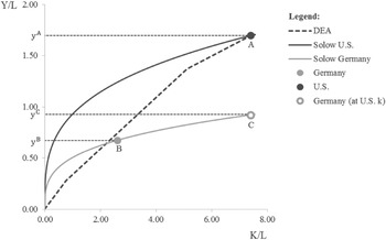
We illustrate the difference between the two approaches using our data for the paper and allied products industry. Appendix Figure 1 shows the labor-productivity and capital-intensity levels of the United States (A) and Germany (B) in this industry in 1935. The figure also displays the global best-practice frontier estimated with DEA and the Solow-based production functions for both countries. With the Solow-based approach, the share of the labor-productivity gap that is attributed to differences in capital intensity equals the labor-productivity increase from y B to y C that results from a move along the German production function from B to C. The remaining labor-productivity gap, i.e., the vertical distance between y C and y A , is then attributed to a difference in TFP.Footnote 5 More formally, in the Solow decomposition of labor productivity gaps:

where the last element on the right-hand side indicates the difference in TFP between the two countries, i.e., the residual labor-productivity gap not explained by differences in capital intensities k. Note that much depends on the choice of the α, which under stringent assumptions represents the capital income share. Typically, this is taken to be 0.3 and this determines the slope of the curves as depicted in Appendix Figure 1.
DEA-BASED AND SOLOW-BASED PRODUCTION FUNCTIONS IN PAPER AND ALLIED PRODUCTS, 1936

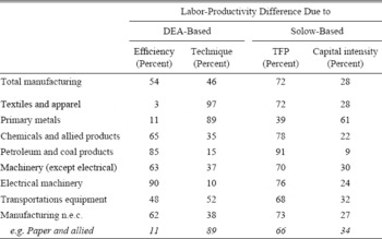
The decomposition with DEA, as illustrated in Figure 3 in the main text, works conceptually similar by measuring the labor-productivity increase that results from a move along the frontier from German to U.S. capital intensities (note that Germany is not on the frontier and hence not fully efficient). The difference, however, is that according to the frontier, the marginal productivity of capital at the German intensity level is much higher than according to the Solow production function. This can be easily seen in the graph by noting the much steeper slope of the tangent line to the frontier than to the Solow functions at the German capital intensity level. This indicates that the labor-productivity pay-off for the same increase in capital intensities is markedly higher according to the DEA approach. Indeed, according to the DEA approach the productivity gap is for 89 percent due to differences in capital intensity, while this only accounts for 34 percent in the conventional approach. So according to the DEA results, German firms could improve labor productivity quickly through further capital intensification and installing new techniques, whereas the Solow-based results suggest that this strategy of further investment would quickly run into high diminishing returns.
What was the actual marginal productivity that German firms faced? The Solow approach seemed to be questionable as it presumes that factor prices reflect marginal productivity (as they would in fully competitive markets). In addition, factor shares are notoriously hard to pin down due to lack of suitable factor price data, in particular in historical studies. For these reasons Broadberry (Reference Broadberry1997, pp. 105–110) rejects the Solow approach. Lacking an alternative he carefully suggested that the α coefficient might be as high as unity, rather than 0.3. Indeed, in the case of the paper and allied industry (Appendix Figure 1) the DEA-based and Solow-based decompositions would return approximately the same results when we assume for the latter an α as high as 0.8.
This result is not particular for the paper and allied industry. Appendix Table 1 contrasts the decomposition results obtained with the DEA-based and Solow-based approaches for major industries.Footnote 6 For almost all industries the DEA-based decomposition allocates a substantially larger share of the labor-productivity gap to differences in capital intensity. This bias in the conventional estimates should not come as a surprise. The DEA approach takes account of the well-known localized nature of technological change. The form of the DEA frontier of 1935 is the culmination of decades of technological change. Innovation was localized and capital biased throughout this period and the frontier moved outward mainly for increasingly higher levels of capital intensity. That is, innovation was predominantly in techniques that were capital intensive as highlighted by Atkinson and Stiglitz (Reference Atkinson and Stiglitz1969), Gary Field (Reference Field1985), and Allen (Reference Allen2012). Labor-intensive techniques were quickly abandoned by the leading industrial nations such that investment-driven strategies appeared to be the prime route to labor productivity catch-up.
DECOMPOSITION OF THE 1936 UNITED STATES/GERMAN LABOR-PRODUCTIVITY RATIO, SOLOW VS. DEA

ONLINE SUPPORTING MATERIAL
Additional supporting material for this article is available online at: http://www.rug.nl/research/ggdc/activities/projecten/mt/yoe/yoe.