Political Scientists face substantial data limitations when measuring public opinion. Much of the research on representation and the role of the public in politics requires good measures of the constituencies to which elected officials are accountable. In the American context, these constituencies may be the residents of a state (who elect their governor and senators), a congressional district (electing their member of the House of Representatives), a state legislative district (electing their member to the state lawmaking body), or any number of other geographically referenced areas that choose a policymaker of consequence. Survey data that provide an estimate of constituency ideology that is not only reliable, but comparable with other districts, are hard to come by. Hence, the discipline of Political Science has had to develop a variety of disparate strategies to address this scarcity of data.
In this methodological work, we develop a new approach for modeling public sentiment by micro-level geographic region based on Bayesian hierarchical spatial modeling using multiple geocoded data sources. Unfortunately, the current state of geographically oriented measurement and modeling in Political Science currently lags behind the stunning amount of raw geospatial political data available for analysis. We seek to resolve this discrepancy with model output that produces nuanced regional relationships and contrasts between constituencies at varying levels, as well as robust district-level aggregations. By exploiting the spatial relationships among observations and units of measurement, we extract measurements of ideology as geographically narrow as available covariate measures. Our approach broadens the process of areal (defined regions) spatial modeling in Political Science by producing a distributed product that allows other researchers to produce aggregation at all practical political levels in American politics: states, congressional districts, census tracts, MSAs, state legislative districts, cities, and counties. This is a new paradigm for spatial political analysis that is flexible on aggregation and draws important information from social, economic, and political information at the most local level.
The end product of this work is a model-based smooth public opinion measure based on the appropriate treatment of hierarchical covariates. To obtain this result, we identify discrete non-nested hierarchies in a collection of data sets and smooth them with Bayesian kriging to produce a model in the form of a posterior density blanket that draws spatial estimates of ideology and other public sentiment from both smoothed geographic terms as well as principled covariates across those levels. By posterior density blanket, we mean a smoothed three-dimensional surface over the area of interest that results from the hierarchical specification along with the Bayesian kriging step, and is smoothed such that the variability of the predictions is less than the variability of the original observations. This density blanket is similar to the spatial relative risk function long employed in spatial epidemiology (Lawson and Williams Reference Lawson and Williams1993; Kellsall and Diggle Reference Kellsall and Diggle1995). The process described accounts for gradual spatial effects rather than arbitrarily sharp effects. This smoothing approach has not been done in the social sciences, even though there are obvious examples where boundaries are not socially determined.
We also generate freely available software that will enable other users to apply any division of interest and obtain smooth measures of latent ideology for their research purposes. Furthermore, the Bayesian hierarchical spatial models developed here can be used for any spatial or areal data analysis process where prediction is important. These models can be customizable beyond geographic measures of public opinion in the United States, given additional relevant data. For this project, the output includes our estimates of state-level ideology, and we also create estimates of congressional districts in Virginia to illustrate the capabilities of our method.
This paper proceeds first by describing the background theory of Bayesian hierarchical spatial modeling. Next, we describe the kind of model we build in order to forecast constituency ideology. Third, we describe the model we use in our current application, given current software limitations. Fourth, we present the forecasts our model produces for 2008 data in the lower 48 states plus the District of Columbia, and in congressional districts in Virginia, along with analyses that show how our measure compares with a simple measure based on survey subunits and multi-level regression with post-stratification. Finally, we discuss the implications of our results and the process for building a more computationally efficient and theoretically robust forecasting algorithm.
Background
Studies in Political Science frequently fail to measure accurately the attributes of areal data units such as congressional districts. This usually means measuring an attribute of a district by weighting measures of component counties by the percentage of their area or weight in the district or, more crudely, simply using the measured value of a district’s largest county while ignoring the fact that district lines are often drawn strategically. For example, if data on average income, voter turnout, religiosity, or any other factor were available at the county level, but not the district level, then a researcher would face this dilemma. Worse yet, political and social boundaries are often non-nested, meaning that there is no systematic hierarchy of geographic units laid out by governments. For instance, congressional districts can cut through counties and cities, census tracts do not tessellate counties, and other non-nested structures exist. This means that researchers are forced to make difficult choices about areal units of analysis in their studies.
In research using American congressional districts as the unit of analysis, the most pervasive measure of electoral ideology is the president’s share of the two-party vote in the district. In principle, the presidential candidates are the same nationwide, so this measure will vary with the location of the median voter in a district. As Kernell (Reference Kernell2009) demonstrates, however, ideologically ranking states or districts using presidential vote shares is only possible when the dispersion of voters is similar, and rating constituencies on a common cardinal scale is impossible with electoral data. Further, voting behavior may be based on a variety of non-ideological concerns that may not be constant across region, thereby inducing measurement error.
In state politics research, a wider variety of measurement techniques has emerged (for a more extensive review of these methods, see Cohen Reference Cohen2006, 6–10). One of the most pervasive techniques is the seminal measurement of state-level ideology by Erikson, Wright and McIver (Reference Erikson, Wright and McIver1993), which pools several CBS News/New York Times polls together to obtain sufficiently large samples for each state. Pooling enough surveys over time requires the assumption that public ideology remains static, an assumption later maintained in several other measures of public sentiment (Lieberman and Shaw Reference Lieberman and Shaw2000; Norrander Reference Norrander2001; Brace et al. Reference Brace, Sims-Butler, Arceneaux and Johnson2002; Park, Gelman and Bafumi Reference Park, Gelman and Bafumi2004; Park, Gelman and Bafumi Reference Park, Gelman and Bafumi2006; Lax and Phillips Reference Lax and Phillips2009). As an alternative perspective, Berry et al. (Reference Berry, Ringquist, Fording and Hanson1998) later made the case that state ideology varies dynamically with a measure based on interest group ratings of congressional candidates, and this alternate view also appears in a wide array of studies (Gray Reference Gray1976; Jacoby and Schneider Reference Jacoby and Schneider2001; Beyle, Niemi and Sigelman Reference Beyle, Niemi and Sigelman2002; Brace et al. Reference Brace, Arceneaux, Johnson and Ulbig2004; Erikson, Wright and McIver Reference Erikson, Wright and McIver2006).
Note, however, that model-based means of measurement, such as the post-stratification technique used by Park, Gelman and Bafumi (Reference Park, Gelman and Bafumi2004), Park, Gelman and Bafumi (Reference Park, Gelman and Bafumi2006), and Lax and Phillips (Reference Lax and Phillips2009) are more amenable to dynamic change than many other techniques for static measurement. In fact, Pacheco (Reference Pacheco2011) illustrates how useful the post-stratification method can be for measuring time-variant state-level opinion. In this paper, we develop a new model-based technique that, similarly, can be used to generate a single static snapshot of opinion or can be fitted over several replicate surveys to create a dynamic measure, as the researcher sees fit. In this way, we develop a measurement strategy that can deal with data limitations that become more severe the smaller the constituency. Further, prior measures do not offer much attention to regional heterogeneity within states, so our technique offers an effective way to spatially model the effects of these discrepancies.
Strategy
The answer to this problem is to create a model-based smooth density blanket for the concept of interest (primarily ideology here) such that arbitrary boundaries are immaterial. We do this with a Bayesian hierarchical spatial model that uses kriging to analyze geocoded survey responses, and then we use this analysis to forecast areal units. A kriging estimate uses an optimized linear combination of the data at observed points to fill-in unobserved points, conditional on the spatial configuration of the observed data and spatial separation between the observed and estimated points (Tam Cho and Gimpel Reference Tam Cho and Gimpel2007; Cressie and Wikle Reference Cressie and Wikle2011), thus producing a smooth density blanket over the complete geographic area of interest with lower variance than the original data. Once this density blanket exists, as determined from a posterior distribution of the chosen outcome and the subsequent smoothing, we and others can create any geographic division that a research question requires by slicing vertically such that divisions remain smooth and separated.
The idea of a smoothed density blanket is illustrated in Figure 1. The rectangular regions on the plane defined by the North–South/East–West dimensions indicate areal units of interest, which could be states, counties, etc. Two regions are highlighted in gray and black for illustration, although in our real analysis the entire United States is analyzed. Now above these two regions is the smoothed density blanket corresponding to the areal boundaries below. Notice that they are smooth at their boundary. Thus, for any region that analysts care about there is a smoothed function in the density dimension that seamlessly joints with that of its neighbors. As an analogy, consider the density blanket to be a sheet of cookie dough. Our algorithms can provide a cookie cutter in any shape that the cook wants. Of course, common “slices” will be by state, county, congressional district, or census tract. In this way, we provide a more realistic approach to modeling spatial variance for political effects.
Smooth surface over two non-overlapping contiguous geographic regions

How Does Our Approach Compare With Conventional Methods?
Three approaches to measuring local-level ideology are particularly pervasive in the literature: subsetting a survey, using election returns, and post-stratification. In the subsetting approach, the researcher simply subsets a large survey by a geographic distinction of interest and aggregates the subsets of data (e.g., Erikson, Wright and McIver Reference Erikson, Wright and McIver1993). There are a couple of problems with this approach. First, the sample size can become quite small in some cases, perhaps to the point of not observing any data for some units (e.g., North Dakota and Wyoming may be states with few or no respondents in a national survey). The second issue is that survey data often are not designed to be representative of a subsample of interest. The American National Election Study, for example, stratifies on region and is therefore not necessarily representative of each state. Hence, state subsamples can be misleading.
A second approach for measuring public sentiment is to use election returns as a proxy for district ideology. The easiest way to examine this is the share of the presidential vote in a district (Erikson and Wright Reference Erikson and Wright1980; Ansolabehere, Snyder and Stewart Reference Ansolabehere, Snyder and Stewart2001). The assumption in this case is that because the candidates’ ideologies are constant nationwide, the vote share will change only in response to the median voter. Alternatively, Berry et al. (Reference Berry, Ringquist, Fording and Hanson1998) create a voting-based measure that uses votes in congressional races, but measures the ideology of both incumbents and challengers to place each district on the same scale. Although vote-based measures use abundant data that are simple to gather, there are concerns with this kind of measure as well. First, vote choice is conceptually distinct from ideology. How an individual behaves at the ballot box may not be based on general ideology, but also regional appeals, personality traits, or economic well-being, thereby inducing added measurement error. Second, the vote share in a district is based solely on who turned out to vote and does not capture the views of non-voters. Finally, vote choice alone may be a misleading measure in that it does not account for the relative dispersion of ideological positions in a district (Kernell Reference Kernell2009).
A third approach seeks to resolve the data limitations and ideological dispersion issues present with the subsetting and proxy methods. Post-stratification models individual responses to survey questions. Then, responses are predicted for every combination of covariates and weighted based on known population quantities for the region of interest (Park, Gelman and Bafumi Reference Park, Gelman and Bafumi2004; Park, Gelman and Bafumi Reference Park, Gelman and Bafumi2006; Tausanovitch and Warshaw Reference Tausanovitch and Warshaw2013). This method draws from weighting techniques also described in Gelman and Little (Reference Gelman and Little1997). Earlier work with such weighting was done by Pool, Abelson and Popkin (Reference Pool, Abelson and Popkin1965), Weber and Shaffer (Reference Weber and Shaffer1972), and Weber et al. (Reference Weber, Hopkins, Mezey and Munger1972). Jackson (Reference Jackson1989), seeking to address the constituency measurement problem, developed a technique wherein a model is fit to national-level survey data and then used to forecast public opinion in small area constituencies using average values of predictors in the constituencies.Footnote 1 Adding these weighted predictions presents an estimate of public ideology that also includes a measure of uncertainty. By resolving many of the problems posed by other measurement strategies, post-stratification presents one of the best means of capturing public ideology by region.
However, we believe that the principle of post-stratification can be further improved upon because no current method of public opinion measurement effectively incorporates the information geography offers. Post-stratification offers a structural model for what shapes individuals’ ideological and issue preferences and the use of such a model to improve estimates of aggregate opinion. Besides observable and measured predictors that shape opinion preferences, though, there may be unobservable factors that shape individuals’ preferences as well. These may be factors such as local discourse, variation in the meaning of partisan labels in local elections, commitment to certain values, membership in labor unions, or any number of other potential factors. Normally, unobservable input variables are relegated to the disturbance term in a model. However, most models assume that each respondent’s disturbance is independent of all other respondents’ disturbances. This assumption is not fair to make.
For a theoretical background on why we expect individuals who are geographically proximate to share similar political attitudes, Gimpel and Schuknecht (Reference Gimpel and Schuknecht2003, 2–4) describe two different approaches to understanding regionalism in politics—a compositional approach and a contextual approach. First, the compositional approach maintains that political behavior bears similarity within a region because economic interests, racial origin, ethnic ancestry, religion, social structure, and other factors tend to be similar among a region’s residents (Gastil Reference Gastil1975; Garreau Reference Garreau1981; Fischer Reference Fischer1989; Lieske Reference Lieske1993). In principle, under the compositional approach, if all of these factors could be included in an empirical model, then individuals’ behavior would not show added similarities once the variables have been accounted for. However, it is often impossible to measure every relevant demographic and socioeconomic variable, or even to identify every relevant input in sufficient detail to include it in a model. (For example, would it be sufficient to know the relative importance of farming and manufacturing in an area, or are unique attributes of different crops and different products also important to regional culture?) As some relevant inputs may be overlooked or unmeasured, it is safer to assume that neighboring individuals will have a relatively similar political outlook, even holding the predictors constant.
The second approach to understanding regionalism, the contextual approach, offers the idea that citizens’ political attitudes and behaviors are influenced by political socialization and by interactions with other citizens in their social network. When citizens influence each other by discussing politics or sharing information, or when they are socialized with similar values, their opinions and actions will tend to be similar (Putnam Reference Putnam1966; Putnam Reference Putnam1993; Huckfeldt and Sprague Reference Huckfeldt and Sprague1995; DeLeon and Naff Reference DeLeon and Naff2004; Djupe and Sokhey Reference Djupe and Sokhey2011). “The first place to look for political networks is within the immediate physical proximity of each individual” (Sinclair Reference Sinclair2012, 26). Therefore, we expect under the contextual approach as well that geographically proximate individuals will have relatively similar opinions, even in a general model.
As empirical support for this point, Erikson, Wright and McIver propose that, “the unique political cultures of individual states exert an important influence on political attitudes” (Reference Erikson, Wright and McIver1993, 48). This notion builds on past work by scholars such as Elazar (Reference Elazar1966), who proposes that states can be categorized based on an individualist, moralist, or traditionalist view of government’s role. Erikson, Wright and McIver (Reference Erikson, Wright and McIver1993, 56–68) proceed to show that a higher proportion of variance in ideology and partisanship can be explained by state-level dummies than by demographic information, though state residuals also will pick up some of the effects of unmeasured individual-level variables. This result also holds in the study of urban areas, where DeLeon and Naff (Reference DeLeon and Naff2004, 703) conclude that political culture shapes the impact of identity on public opinion and political participation. It appears, then, that citizens in nearby locales do share a similar political outlook.
Our method of kriging increases the ability to reasonably capture the effects of political culture, omitted predictors, and social context by including weighted neighbors’ residuals in forecasts of public opinion. In neighboring regions, residents are likely to share a similar political culture, similar values of unobserved predictors, and similar political socialization. For example, western Kentucky and southeast Illinois are similar places that are likely to be populated with similar people, both in cultural and demographic terms. However, none of the three aforementioned approaches explicitly attempts to capture this in the measurement strategy.
Provided that geographically proximate citizens do share similar political views, then kriging will improve upon current measurement strategies in three ways. First, the kriging approach improves estimates of the structural model of individual opinion relative to methods like post-stratification. By dropping the assumption that each individual’s response is independent of all others, we allow the disturbances in individuals’ responses to survey questions to covary conditionally on how geographically proximate they are. Doing this yields more efficient parameter estimates than the wrongful assumption that the disturbances are independent. Hence, the predictive structural model ought to be more accurate.
Second, in the process of allowing spatial autocorrelation, we estimate a surface of what the spatial random effects are (see again Figure 1). By fitting this kriging surface and then using the values of this surface to predict ideology or issue opinion in a region, the added information will further raise the quality of our predictions. To the degree that unmeasured variables and political culture shape public opinion, the crafting of this surface ought to better incorporate these features into the forecast. Regardless of how small the constituency’s area is, a reasonable projection of these factors is incorporated via kriging. As the kriging surface is identified through the spatial location of each respondent, fitting this surface allows us to separate the variance not explained in the mean model into variance that spatially clusters and variance that is truly stochastic. This further reduction of variance that cannot be used in prediction improves our measures.
Third, every forecast should report a level of uncertainty in prediction. In our case, this takes the form of credible surfaces around the kriged density blanket. Predictions for larger areas (such as entire states) will be more certain than predictions for smaller areas (such as congressional or state legislative districts), and so these credible surfaces on either side of the estimate will be smaller in the former case. Naturally, the same would hold for any other method, including survey disaggregation and post-stratification, but by including the information of the spatial surface in our model and predictions, we can reduce the error of our areal predictions to be as small as possible, whereas providing accurate measures of uncertainty at any level of aggregation.
Model Overview
The first stage is to specify a Bayesian hierarchical model that accounts for aggregation in the data that we will use: individuals (in our case, survey respondents) are nested in regions, and the regions have associated covariates. These multi-level approaches make sure that the levels in the data are treated appropriately in the model and we do not assign regional or nesting variables directly to individuals (Gelman and Hill Reference Gelman and Hill2007; Gill and Womack Reference Gill and Womack2012).
Basic Spatial Specification
Consider X*, an n×k positive definite matrix of explanatory variables organized down columns with a leading column of ones. Denote for the ith case, xij is a vector of explanatory variable values, and the j index is a reminder of nesting in the jth regional group. Furthermore, partition the n×k matrix X* into two submatrices that track the nesting distinction:
 $$\mathop{{{\bf X}^{{\asterisk}} }}\limits_{{n{\times}k}} =\left[ {\mathop{{\bf X}}\limits_{{n{\times}p}} \,{\vskip12pt\rot90{-\!\!\!-\!\!\!-\!\!\!-\!\!\!-\!\!\!-}}\mathop{{\bf Z}}\limits_{{n{\times}q}} } \right],$$
where X is the matrix of variables that will have unmodeled coefficients (receiving standard point estimates) and Z the matrix of explanatory variables that will have modeled coefficients through a hierarchy and therefore will be described distributionally. Finally, specify an error structure, ϵ, containing ϵ ij values that are all independent and identically distributed according to  $$\epsilon _{{ij}} \,\sim\,{\cal N}_{n} (0,\,\sigma ^{{\rm 2}} )$$
, σ 2>0. The complete model for our outcome is now the simple form:
 $${\bf Y}={\bf X}\bibeta {\plus}{\bf Zu}{\plus}\epsilon ,$$
where β is a p-length vector of coefficient estimates and u the q-length vector of random effects with the assumption of multivariate normality with mean zero and positive definite variance–covariance matrix, such that  ${\bf u}\,\sim\,{\cal N}_{q} (0,\Delta )$
. This produces a method of accounting for structured data through regression equations at different hierarchical levels in the data. These higher-level models are describing distributions at the level just beneath them for the coefficient that they model as if it were itself an outcome variable. In this way, multi-level models are highly symbiotic with Bayesian specifications because the focus in both settings is on making supportable distributional assumptions.
This hierarchical approach models the systematic component, but does not yet incorporate the smoothing that we require for our purposes. The latter is done with kriging through the variance component of the model. For simplicity, label μ=Xβ+Zu in (2) above and generalize the variance component according to:
 $$\Sigma =\sigma ^{2} {\bf H}(\phi ){\plus}\tau ^{2} {\bf I},$$
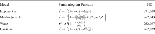
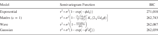
where σ 2 is a weight, called the partial sill, H(ϕ) an n×n correlation matrix where the ijth value is defined by a parametric function, and τ 2 another weight, called the nugget, that multiplies an n×n identity matrix (τ 2+σ 2 is called the sill). In this context, ϕ is called the decay parameter, and 1/ϕ is called the range parameter. The ijth off-diagonal values of H actually could follow a variety of functional forms called covariograms (assumed spatial covariances at fixed distances), such as the wave, Gaussian, or Matérn functions, depending on what fits the data best (see Table 1 for a summary of some semivariograms). Often these parametric forms are given simple forms like exp(ϕd ij), an exponential correlation function, where the values d ij are coordinate-based distance measures between case i and case j, weighted by autocorrelation parameter ϕ. These terms originate from Cressie (Reference Cressie1991), and are further described in Banerjee, Carlin and Gelfand (Reference Banerjee, Carlin and Gelfand2004).
Four Candidate Parametric Semivariograms and their Relative Fit
Note: N=21,543. Data from 2008 Cooperative Congressional Election Study. Notation from Banerjee, Carlin and Gelfand (Reference Banerjee, Carlin and Gelfand2004, table 2.2). Bayesian information criterion (BIC) formula drawn from Gujarati and Porter (Reference Gujarati and Porter2009, 494). Computed with the geoR 1.7-4 library in R 3.0.0.
The model is not yet complete, so modify it to specify a correlation at the group level:
 $${\bf Y}\,\mid\,\mu ,\sigma ^{2} ,\tau ^{2} ,\phi \,\sim\,{\cal N}({\bf X}\beta {\plus}{\bf Zu}{\plus}{\bf W},\tau ^{2} {\bf I}),$$
thus adding a vector of spatial random effects:
 $${\bf W}=\{ w(s_{1} ),w(s_{2} ),\,\,\ldots\,\,,w(s_{n} )\} ,$$
such that each Y(si) is conditionally independent given the w(si) and ui, where si is a vector of location coordinates for observation i. The spatial aspect of the hierarchy is now given by:
 $${\bf W}\,\mid\,\sigma ^{2} ,\phi \,\sim\,{\cal N}(\bf0,\sigma ^{2} {\bf H}(\phi )),$$
where H(ϕ)ij=ρ(ϕ,||si−sj||) and ρ a spatially appropriate correlation function. The spatial density blanket is now a function of W|Y, which naturally leads to credible intervals. Putting the hierarchical component together with the kriging component, along with a multivariate normal assumption, gives the full model. Hence, we now have a complete model of individual survey respondents that accounts for the respondents’ locations in latitude and longitude. With this model in hand, we will use the technique of point-to-block realignment (spatial forecasts at new locations) to measure public sentiment for border-referenced constituencies (Banerjee, Carlin and Gelfand Reference Banerjee, Carlin and Gelfand2004, chapter 6). This model-based approach better accounts for dissimilarities across politically drawn lines and yields estimates with less measurement error as arbitrary boundaries like census tracts do not separate responses. Instead, the distance-based model recognizes shared effects by geography along with distinct effects by model hierarchy.
As a final point on background, Banerjee, Carlin and Gelfand (Reference Banerjee, Carlin and Gelfand2004) give GeoBUGS code for specifying point-referenced models similar to what we have described. However, GeoBUGS is designed as an add-on package for WinBUGS, which only works on the Windows operating system. Further, GeoBUGS has proven to be computationally inefficient for these types of models and unable to handle large data sets effectively. Hence, we currently implement this structure using R.
Model for Unobserved Spatial Points
Our fundamental goal is to model the opinions of individuals, who are located in latitude and longitude, and use the information from this model to measure the ideology of a whole constituency. In this vein, Banerjee, Carlin and Gelfand (Reference Banerjee, Carlin and Gelfand2004, 179–80) describe the method for using observations taken at various points in latitude and longitude and realigning them into measures of block-level averages. Their design assumes that the observed point-level data and the extrapolated block-level averages have a joint Gaussian distribution. If survey data include the latitude and longitude of survey respondents’ residences (or, more commonly, information like ZIP code, for which coordinates can be assigned with reasonable accuracy), then point-to-block realignment offers an opportunity for effective measurement of precincts or congressional districts.
We want to create a posterior density blanket for some outcome of interest for the entire United States that can be sliced by any districting method where the partition is available. In the case of ideology, this would be an extension of Erikson, Wright and McIver (Reference Erikson, Wright and McIver1993), where the boundaries are not required to be US states. This means that the final result will include estimates for spatial points where there is no observed data. Define now s as a set of n observed sites {s1, s2, … , sn}, where Y(s) is an associated collection of outcomes Y(s)={Y(s1), Y(s2), … ,Y(sn)} and X*(s)={x*(s1), x*(s2), … ,x*(sn)} is a collection of hierarchical covariates at those points. Note that the X*(s) are conditional on the level of aggregation chosen (state, county, congressional district, etc.). Now alter the linear specification in (2) to accommodate this new setting:
 $${\bf Y}({\bf s})=\mu ({\bf s}){\plus}\omega ({\bf s}){\plus}\epsilon ({\bf s}),$$
where μ(s)=X(s)β+Z(s)u is the mean structure based on a linear additive component, ω(s) the realizations from a mean zero stationary (usually) Gaussian spatial process that captures spatial association (includes the partial sill σ 2 and the range ϕ), and ϵ(s) a regular uncorrelated disturbance term (includes the nugget effect τ 2, its variance). In addition, assume that  $$\omega \left( {\bi s} \right)\!\sim\!{\cal N}(\bf0,\bisigma ^{{\rm 2}} {\bf H}(\phi ))$$
and
 $$\epsilon \left( {\bf s} \right)\sim{\cal N}(\bf0,{\rm }\tau ^{{\rm 2}} {\bf I})$$
.
As noted, we usually specify the correlation function of ω(s) to be a function of the separation between points to give a stationary model, so that:
 $$\mu ({\bf s})=E[Y({\bf s})]{\rm \ and}\ f({\rm Var}({\bf s}))=f({\rm Var}({\bf s}{\plus}{\bf h})),\,{\rm for}\,{\rm any}\,{\bf h}\in \Re ^{r} ,\;r\leq n,$$
where h is called the separation vector, and f() an arbitrary user-defined function (which also just be the identity function). If this separation is purely based on distance, ||si−sj||, then we get isotropy, meaning that the semivariogram function
 $$\gamma ({\bf h})={1 \over 2}{\rm Var}({\bf Y}({\bf s}{\plus}{\bf h}){\minus}{\bf Y}({\bf s})),$$
depends on h only through its length ||h||. In this context, the nugget can be thought of as micro-scale variability: variability at distances smaller than the smallest inter-location distance in the data. This is important as we are now making predictions about points and distances between points that are not in the original data. Figure 2 gives an example of an exponential form.
Exponential semivariogram where τ2=0.1, σ 2=0.9, and ϕ=1
We clearly want the posterior distribution of the coefficient vector β for regression purposes, as well as the parameters σ 2, τ 2, and ϕ. However, we also want a smooth density blanket for Y(s), which requires predictions at unobserved sites, generically labeled s0, giving Y(s0) values at chosen locations. Kriging actually has two steps that are important here: the process of applying mathematical decision criteria, and then applying constrained optimization to get a density blanket. We consider this problem in the context of Gaussian processes, but many other distributional frameworks are available.
Optimization Criteria
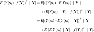
The method of point-to-block realignment calls for kriging, or making forecasts of a spatially referenced variable (ideology, in our case) at new geographic locations. When choosing a kriging function with which to make forecasts, an obvious decision criterion is to find a function f(Y) that minimizes the mean squared prediction error:
 $$\eqalignno{ E[(Y({\bf s}_{0} ){\minus}f({\bf Y}))^{2} \,\mid\,{\bf Y}]= \,& E[((Y({\bf s}_{0} ){\minus}E[Y({\bf s}_{0} )\,\mid\,{\bf Y}]) \cr &{\plus}(E[Y({\bf s}_{0} )\,\mid\,{\bf Y}]\,{\minus}\,f({\bf Y})))^{2} \,\mid\,{\bf Y}] \cr =\, & E[(Y({\bf s}_{0} ){\minus}E[Y({\bf s}_{0} )\,\mid\,{\bf Y}])^{2} \,\mid\,{\bf Y}] \cr & {\plus}E[(E[Y({\bf s}_{0} )\,\mid\,{\bf Y}]\,{\minus}\,f({\bf Y}))^{2} \,\mid\,{\bf Y}]. $$
However,  $$E\left[ {(E[Y({\bf s}_{0} )\,\mid\,{\bf Y}]\,{\minus}\,f({\bf Y}))^{2} \,\mid\,{\bf Y}} \right]$$
has to be non-negative because of the square, so we know that
 $$\eqalignno{ & E\left[ {(Y({\bf s}_{0} ){\minus}E[Y({\bf s}_{0} )\,\mid\,{\bf Y}])^{2} \,\mid\,{\bf Y}} \right]{\plus}E\left[ {(E[Y({\bf s}_{0} )\,\mid\,{\bf Y}]\,{\minus}\,f({\bf Y}))^{2} \,\mid\,{\bf Y}} \right] \cr & \geq E\left[ {(Y({\bf s}_{0} ){\minus}E[Y({\bf s}_{0} )\,\mid\,{\bf Y}])^{2} \,\mid\,{\bf Y}} \right]. $$
The minimum (as in equality, not inequality above) happens only when f(Y)=E[Y(s0)|Y], meaning E[Y(s0)|Y] is the function that minimizes mean squared prediction error. We know that E[Y(s0)|Y] is the posterior mean of Y(s0) and therefore minimizes the posterior risk with a squared error loss function. Furthermore, an estimator that minimizes the Bayesian posterior risk is one that for every  $Y\in {\cal Y}$
specifies a decision rule, d(Y), that minimizes the posterior expected loss,
 $$E_{\pi } [{\Bbb L}(A,d({\bf Y}))]$$
, for action A. This is an overtly Bayesian statement of loss as we are averaging over uncertainty in the posterior distribution of β, not over the distribution of data since it has already been observed. The subsequent decision rule which minimizes:
 $$R_{B} (\bibeta ,d({\bf Y}))=\mathop{\int}_{B} \mathop{\int}_{\cal Y} {\Bbb L}(A,d({\bf Y}))dF_{{\cal Y}} (y\,\mid\,\bibeta )dF_{\pi } (\bibeta ),$$
for every  $Y\in {\cal Y}$
is called optimal, and limiting the set to this choice is called a Bayes rule, denoted
 $$\widehat{{R_{B} }}(\beta ,d({\bf Y}))$$
here, and defined by the function minimizing value of β A that satisfies:
 $$\widehat{{R_{B} }}(\beta ,d({\bf Y}))=\mathop{{\inf }}\limits_{{\beta _{A} }} \mathop{\int}_{B} R_{F} (A,d({\bf Y}))dF_{\pi } (\beta ),$$
(Gill Reference Gill2014). This is then our criteria for finding β in (4). We describe a Markov chain Monte Carlo (MCMC) process for estimating the parameters in Appendix A, and this algorithm represents a large proportion of the contribution of this work.Footnote 2
Data Application: Measuring Public Ideology in 2008
Recall that our objective is a measure of public opinion (ideology and other public sentiment) for constituencies from both smoothed geographic terms as well as covariates. These are almost always areal or block units: states, congressional districts, state legislative districts, precincts, etc. Furthermore, survey data are typically sparse at the subnational level, and aggregated measures such as presidential vote share also pose problems (Kernell Reference Kernell2009). The best way to address these challenges is through an overtly hierarchical specification that references individual survey respondents, but adds covariate information at higher levels of aggregation (similar to past model-based methods, e.g., Pool, Abelson and Popkin Reference Pool, Abelson and Popkin1965; Weber and Shaffer Reference Weber and Shaffer1972; Weber et al. Reference Weber, Hopkins, Mezey and Munger1972; Jackson Reference Jackson1989; Park, Gelman and Bafumi Reference Park, Gelman and Bafumi2006). Recognizing these differing levels in the model means that we can add extra information based on geographic location for any desired constituency.
Parameter Choices
As our model assumes the observed point-level data and the extrapolated block-level averages have a joint Gaussian distribution, we get:
 $$f\left( {\left( {\matrix{ {{\bf Y}_{{\bf s}} } \cr {{\bf Y}_{{\bf B}} } \cr } } \right)\,{\vskip12pt\rot90{-\!\!\!-\!\!\!-\!\!\!-\!\!\!-\!\!\!-}}\,{\bibeta ,\sigma ^{2} ,\phi }} \right)={\cal N}\left( {\left( {\matrix{ {\mu _{{\bf s}} (\bibeta )} \cr {\mu _{{\bf B}} (\bibeta )} \cr } } \right),\sigma ^{2} \left( {\matrix{ {{\bf H}_{{\bf s}} (\phi )} & {{\bf H}_{{{\bf s},{\bf B}}} (\phi )} \cr {{\bf H}_{{{\bf s},{\bf B}}}^{T} (\phi )} & {{\bf H}_{{\bf B}} (\phi )} \cr } } \right)} \right),$$
where Ys represents the vector of ideology among individual citizens, YB the vector of ideology in all block-referenced constituencies of interest, and H the correlation matrix of observations as before. Note that this presents the simplified case where there is no nugget effect (τ 2), but the result still holds if the variance–covariance terms do include a nugget, as seen in Appendix A. By standard normal theory (e.g., Ravishanker and Dey Reference Ravishanker and Dey2002), the conditional distribution of our extrapolated block averages is:
 $$\eqalignno{ {\bf Y}_{{\bf B}} \,\mid\,{\bf Y}_{{\bf s}} ,\bibeta ,\sigma ^{2} ,\phi \,\sim\, & {\cal N}(\mu _{{\bf B}} (\bibeta ){\plus}{\bf H}_{{{\bf s},{\bf B}}}^{T} (\phi ){\bf H}_{{\bf s}}^{{{\minus}1}} (\phi )({\bf Y}_{{\bf s}} \,{\minus}\,\mu _{{\bf s}} (\bibeta )), \cr & \sigma ^{2} [{\bf H}_{{\bf B}} (\phi ){\minus}{\bf H}_{{{\bf s},{\bf B}}}^{T} (\phi ){\bf H}_{{\bf s}}^{{{\minus}1}} (\phi ){\bf H}_{{{\bf s},{\bf B}}} (\phi )]). $$
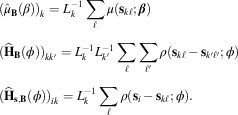
These quantities can be estimated with Monte Carlo integration:
 $$\eqalignno{ & (\hat{\mu }_{{\bf B}} (\beta ))_{k} =L_{k}^{{{\minus}1}} \mathop{\sum}\limits_\ell \mu ({\bf s}_{{k\ell }} ;\bibeta ) \cr & ({\bf \widehat{H}}_{{\bf B}} (\phi ))_{{kk'}} =L_{k}^{{{\minus}1}} L_{{k'}}^{{{\minus}1}} \mathop{\sum}\limits_\ell \mathop{\sum}\limits_{\ell '} \rho ({\bf s}_{{k\ell }} \,{\minus}\,{\bf s}_{{k'\ell '}} ;\phi ) \cr & ({\bf \widehat{H}}_{{{\bf s},{\bf B}}} (\phi ))_{{ik}} =L_{k}^{{{\minus}1}} \mathop{\sum}\limits_\ell \rho ({\bf s}_{i} {\,\minus\,}{\bf s}_{{k\ell }} ;\phi ). $$
This will allow us to forecast the average ideology with:
 $$\hat{\mu }_{{\bf B}} (\bibeta ){\plus}{\bf \widehat{H}}_{{{\bf s},{\bf B}}}^{T} (\phi ){\bf \widehat{H}}_{{\bf s}}^{{{\minus}1}} (\phi )({\bf Y}_{{\bf s}} \,{\minus}\,\hat{\mu }_{{\bf s}} (\bibeta )).$$
We account for the spatial element by forecasting  $$\hat{Y}({\bf s}_{{k\ell }} ;\bibeta ,\sigma ^{2} ,\tau ^{2} ,\phi )$$
and using this quantity in our Monte Carlo integration. With the nugget effect, from Y(s)=μ(s)+ω(s)+ϵ(s), we also get
 $${\bf Y}_{{\bf s}} \sim{\cal N}(\bimu ,\,∑)$$
, where we still require ∑=σ 2H(ϕ)+τ 2I, H(ϕ)ij=ρ(ϕ, d ij) and d ij=||si−sj||. For this application, we selected the Gaussian semivariogram function for reasons shown below.
We want to forecast blocks using the conditional distribution in (12). However, current software is inadequate to jointly estimate the geospatial model and krige for more than a few kriged points, and there is no ability to obtain the conditional block averages. As a result, we developed our own sampler to more efficiently allow for kriging over a wide number of locations and more directly model the conditional mean of blocks (Appendix A).
Data for 2008
As our training data for this model we use the 2008 Cooperative Congressional Election Study (CCES) (Ansolabehere Reference Ansolabehere2011). These data offer 21,543 observations spread across the American states and congressional districts, and the variables are described in Appendix B. Further, the data report ZIP codes, allowing us to place respondents in geographic space.Footnote 3Figure 3 presents the geographic location of the respondents in the training data. The locations are presented on a scale of eastings and northings, which accounts for the spherical shape of the earth and places all observations on a common kilometer-referenced scale. By contrast, a degree of latitude need not constitute the same distance as a degree of longitude.Footnote 4
Geographic locations in kilometer-referenced eastings and northings of survey respondents in the 2008 Cooperative Congressional Election Study
The CCES presents a 100-point self-reported ideology scale, which serves as the outcome of interest.Footnote 5 It also provides covariates for age, education, race, sex, family income, religion, employment status, and homeowner status. We also include urban–rural status as a predictor by linking respondents’ respective counties to the US Department of Agriculture’s (USDA) scale for the relative ruralness of a county (USDA 2004). Lastly, with the eastings and northings generated by ZIP code, we include a polynomial function of location as a predictor.
When forecasting for states and congressional districts, we draw most covariates by sampling from the population distribution for the ZIP code in which the kriged point falls in, thereby drawing covariates consistent with the local population. We use the complete 2000 Census data, drawing from the joint distribution of age, race, and sex, and then drawing from the conditional distribution for all other predictors given these demographics. ZIP code-referenced Census data were archived with the National Historic Geographic Information System (Minnesota Population Center 2011).Footnote 6 For urban–ruralness, each kriged location in space is linked to the USDA county score. Moreover, as Census does not report religion, we independently draw from each county’s distribution of religious adherents using the 2000 Religious Congregations and Membership Study (Jones et al. Reference Jones, Doty, Grammich, Horsch, Houseal, Lynn, Marcum, Sanchagrin and Taylor2002; Finke and Scheitle Reference Finke and Scheitle2005).Footnote 7 Thus, for a given kriged point, there is demographic information based on the ZIP code the point falls in, and we draw information on religiosity and ruralness based on the county in which the point falls.
Model Specification and Estimation
In addition to our predictors of age, education, race, sex, income, religion, employment status, homeowner status, and urban–rural status, our model of mean ideology also includes a spatial trend term. The spatial trend surface is a linear combination of polynomials of the spatial coordinates. Following the prescription of Cressie (Reference Cressie1993, 155–6), the polynomial terms are defined by the formula:
 $$\mathop {\mathop{\sum} \mathop{\sum} }\limits_{0\leq k{\plus}\ell \leq r} \alpha _{{k\ell }} s_{{i1}}^{k} s_{{i2}}^{\ell } ,\quad {\bf s}_{i} =(s_{{i1}} ,s_{{i2}} )',$$
where si is the vector location of observation i, s i1 the easting for observation i, s i2 the northing for observation i, α kl the coefficient for the term where the easting is raised to the exponent k and the northing is raised to the exponent l, and r the order of the polynomial trend term. In short, for an rth-order trend surface, every product term for which the exponents on eastings and northings sum to any quantity ≤r is included. After comparing the fit of models including a constant trend (r=0) up through a fourth-order trend (r=4) using Schwarz’s Bayesian information criterion (BIC), we found that the second-order and third-order models fit the best. Owing to multicollinearity issues, simplicity in reporting, and a slightly better penalized fit, we present the results of the second-order model (r=2).Footnote 8
With this linear structure in place for the model of ideology’s mean, the full Bayesian model can be specified as follows:
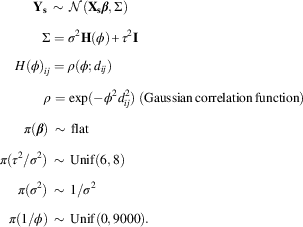 $$\eqalignno{& \ \ \ \ \ \ \ \,{\bf Y}_{{\bf s}} \,\sim\,{\cal N}({\bf X}_{{\bf s}} \bibeta ,\Sigma ) \cr & \ \ \ \ \ \ \ \ \ \,\Sigma =\sigma ^{2} {\bf H}(\phi ){\plus}\tau ^{2} {\bf I} \cr & \ \ \ \,H(\phi )_{{ij}} =\rho (\phi ;d_{{ij}} ) \cr & \ \ \ \ \ \ \ \ \ \ \rho =\exp ({\minus}\phi ^{2} d_{{ij}}^{2} )\;{\rm (Gaussian}\,{\rm correlation}\,{\rm function)} \cr & \ \ \ \ \ \,\pi (\bibeta )\,\sim\,{\rm flat} \cr & \pi (\tau ^{2} /\sigma ^{2} )\,\sim\,{\rm Unif}(6,8) \cr & \ \ \ \ \pi (\sigma ^{2} )\,\sim\,1/\sigma ^{2} \cr & \ \ \pi (1/\phi )\,\sim\,{\rm Unif}(0,9000). $$
In this setup, rather than modeling the nugget effect (τ 2) directly, we model the relative nugget (τ 2/σ 2) or ratio of the nugget to the directly modeled partial sill. As a reasonably tight prior is required for numerical stability (Hobert and Casella Reference Hobert and Casella1996), we centered a uniform distribution around an ∼7:1 empirical ratio of these two quantities. For the partial sill (σ 2), we assume a reciprocal prior, and for the range (1/ϕ), we assume a uniform prior up to twice the maximum distance in the data. Priors on the regression coefficients are flat. The best-fitting covariance function is the Gaussian function, which will be described more in the next section, and all other model attributes are defined as before.
To estimate this model, we adapt a five-step algorithm developed by Diggle and Ribeiro (Reference Diggle and Ribeiro2002, 141).Footnote 9 First, we draw several values from a discrete version of the uniform priors for  $${{\tau ^{2} } \over {\sigma ^{2} }}$$
and
 ${1 \over \phi }$
. Second, we estimate the conditional posterior distribution,
 $$p\left( {{{\tau ^{2} } \over {\sigma ^{2} }},\,{1 \over \phi }\,\mid\bf Y} \right)$$
by placing our draws from the discrete prior into the following formula:
 $$p\left( {{{\tau ^{2} } \over {\sigma ^{2} }},{1 \over \phi }\,\mid\,{\bf Y}} \right)\propto\pi \left( {{{\tau ^{2} } \over {\sigma ^{2} }}} \right)\pi \left( {{1 \over \phi }} \right)\,\mid\,V_{{\tilde{\beta }}} \,\mid\,^{{{1 \over 2}}} \left| {{\bf H}(\phi ){\plus}\left( {{{\tau ^{2} } \over {\sigma ^{2} }}} \right){\bf I}} \right|^{{{\minus}{1 \over 2}}} (\hat{\sigma }^{2} )^{{{\minus}{n \over 2}}} ,$$
where  $V_{{\tilde{\beta }}} $
is the correlation matrix of the regression coefficients estimated with generalized least squares (GLS) using the current draw of 1/ϕ, n the sample size, and
 $$\hat{\sigma }^{2} $$
an estimate of the partial sill based on residuals drawn from the GLS coefficient estimates.Footnote 10 All other terms are defined as before. Third, we draw a single set of sample posterior values for
 $${{\tau ^{2} } \over {\sigma ^{2} }}$$
and
 ${1 \over \phi }$
from (16). Fourth, we attach the set of sampled values to
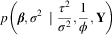 $p\left( {\bibeta ,\sigma ^{2} \,\mid\,{{\tau ^{2} } \over {\sigma ^{2} }},{1 \over \phi },\bf Y} \right)$
and compute the corresponding conditional posterior distributions as:
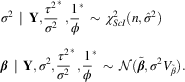 $$\eqalignno{ & \sigma ^{2} \,\mid\,{\bf Y},{{\tau ^{2} } \over {\sigma ^{2} }}^{{\asterisk}} ,{1 \over \phi }^{{\asterisk}} \,\sim\,\chi _{{ScI}}^{2} (n,\hat{\sigma }^{2} ) \cr & \bibeta \,\mid\,{\bf Y},\sigma ^{2} ,{{\tau ^{2} } \over {\sigma ^{2} }}^{{\asterisk}} ,{1 \over \phi }^{{\asterisk}} \,\sim\,{\cal N}(\tilde{\bibeta },\sigma ^{2} V_{{\tilde{\beta }}} ). $$
Here, the term χ 2Scl refers to the Gaussian-Scaled-Inverse-χ 2 distribution. The terms in these equations are again drawn from the GLS estimates from the initial draw of ϕ. After taking a draw from the scaled inverse χ 2 distribution for the partial sill σ 2, this term is linked with the draws from the relative nugget and range terms when drawing the regression coefficients from a normal distribution. By repeating the third and fourth steps to generate a sufficiently large sample from each of the conditional posteriors, we build a sufficient Monte Carlo sample to reflect the joint posterior for the full parameter set  $\left( {{{\tau ^{2} } \over {\sigma ^{2} }},{1 \over \phi },\sigma ^{2} ,\bibeta } \right)$
.
Results
Appendix C reports the results of a simple linear model of self-reported ideology on a 0 (liberal) to 100 (conservative) scale, estimated with ordinary least squares (OLS). This model previews our structural perspective of modeling ideology as a function of demographics recorded in Census data. Following Park, Gelman and Bafumi (Reference Park, Gelman and Bafumi2004), we include the predictors of age, education, race, and sex. We also add income, religion, ruralism, homeownership, and employment status as demographic predictors. (Hence, all of these are individual-level variables except for ruralism, which is a county-level variable.) Per the discussion of Equation (14), we also include a second-order polynomial trend of ideology based on the survey respondent’s location in eastings and northings. This aspect allows the ideology mean to vary by region in a globally defined way. Our subsequent model will make the assumption that, once this trend has been removed, additional localized spatial clustering can be captured through a model of the error variance.
Figure 4 presents the empirical semivariogram of our data. The horizontal axis represents the distance separating survey respondents in kilometers, and the vertical axis reports the semivariance among observations spread that far apart. In this figure, the distance between two observations is the Euclidean distance based on the two-dimensional coordinates of eastings and northings: each point on the figure represents the estimated semivariance among a bin of observations separated by approximately the distance on the horizontal axis. The semivariance can be interpreted as either half the variance of the differences in the outcome over a certain separation of length ||h|| (e.g., 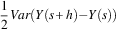 $${1 \over 2}Var(Y(s{\plus}h){\minus}Y(s))$$
), or the full variance of the level of the outcome given this distance (e.g., Var(Y| ||h||)) (Matheron Reference Matheron1963; Cressie and Hawkins Reference Cressie and Hawkins1980). The open points represent the semivariance for the raw, unmodeled observations of ideology. The plus signs represent the semivariance for the residuals from a linear model estimated with OLS. Naturally, the variance of the residuals is consistently smaller owing to some variance being explained by the model.
Empirical semivariogram of respondent ideology in 2008 Cooperative Congressional Election Study Note: Circles show the empirical semivariogram for unmodeled ideology, plus signs show the empirical semivariogram for residuals of ideology from a linear model, and the line shows the fitted Gaussian semivariogram from a jointly estimated Bayesian model.
As is expected of spatially referenced data, more proximate observations have smaller variance, indicating that they are more highly correlated. As distance increases, the semivariance increases as the observations become more independent of each other. As a comparison, the semivariance of unmodeled observations with no separation is ~675, meaning that the variance in ideology scores among respondents with no spatial separation is 675. By contrast, among observations separated by ~3300 km, the semivariance is over 720: this means that the variance in ideology scores among respondents separated by 3300 km is 720, and the variance of the differences, Y(s+h)−Y(s), when ||h||=3300 is 1440. In using this graph to choose a parametric semivariogram in specifying the complete spatial model, we compare the patterns in the raw semivariogram to the empirical signature produced by several common parametric forms.Footnote 11 We observed that a Gaussian semivariogram function best fit the pattern of the raw data, and wave function looked more appropriate for the residuals.
Table 1 describes the four commonly used semivariogram specifications that we considered for our analysis. The wave, Matérn, and Gaussian functions were the most plausible because these three allow the decay in spatial correlation to accelerate at intermediate distances. (This is exemplified in Figure 4 by the fact that the variance stays fairly low up to around 2000 km, then rapidly rises.) As a point of reference, we also estimate the functionally simple and widely used exponential semivariogram function. As the table shows the Gaussian model had the lowest BIC value, indicating the best fit. The exponential, by contrast, fit far worse than the other three candidates. As the simplest and best-fitting model, we proceed with the Gaussian semivariogram function.
With this sense of the structure of spatial correlation, we turn to a model that estimates the mean and error structure simultaneously. Current software is limited in its ability to process massive amounts of spatial data, so we introduce the technique of Bootstrapped Random Spatial Sampling (BRSS) to estimate the full model. We proceed by drawing 100 subsamples with replacement from the full data. Each sample consists of 5 percent of the original data. We then run the Monte Carlo sampler described in the previous section on each subset, save 1000 iterations, and pool the results across all 100 subsamples. Appendix C reports the results of this estimation with posterior means, standard errors, and credible intervals from the Monte Carlo integration process.Footnote 12 Many of the results are substantively similar to the OLS findings from before. However, the estimates of the coefficients have become more diffuse. In addition, the estimates of the variance terms differ somewhat, with a smaller nugget effect and range term.Footnote 13 The posterior mean for the nugget effect (τ 2) indicates that the non-spatial unexplained variance is around 605, whereas the posterior mean for the partial sill (σ 2) indicates that the spatial unexplained variance is around 87. With ~12.6 percent of the unexplained variance accounted for by space, spatial smoothing appears to add a substantial degree of explanatory power.
Again, Figure 4 presents the original unconditional semivariogram and the semivariogram of OLS residuals. The line in this figure presents the Gaussian semivariance function using the posterior means of the BRSS. The Bayesian model simultaneously estimates the regression coefficients and spatial covariance parameters, so the reported line ought to better reflect the spatial correlation. Relative to the empirical semivariogram of OLS residuals reported in the figure, we see a stronger correlation at lower distances and a weaker one at farther distances, which is theoretically sound.
Forecasts for the Lower 48 States and DC
We proceed to estimate the ideology of the lower 48 states and Washington, DC in four steps. First, we draw points from across the United States, link each point with its corresponding state, and pair the point with a random draw of demographic data from the 2000 Census for the relevant ZIP code. When simulating citizens, we sample first by ZIP code in proportion to the population of the ZIP code, then randomly draw a location around the ZIP code’s centroid. In this manner, the geographic distribution of our simulated points reflects the geographic distribution of population in the United States. During this stage, we create 241,530 simulated citizens who are assigned a specific location in latitude and longitude as well as all covariate values. Second, for every iteration of our Monte Carlo sample, we draw 5 percent (or 12,076) of these simulated voters with replacement. Third, we use the parameter values at the given iteration to forecast ideology for the 12,076 simulated citizens with the 5 percent of the data used to fit the particular iteration. Fourth, after kriging ideology for every iteration of the sample, we average the ideology of all of the kriged points within a state.
We present our estimates in Figure 5. Figure 5(a) shows a map of our estimates, with darker values indicating that citizens in the state are more conservative than in the average state and lighter values indicating that they are more liberal. As a contrast to our estimate, Figure 5(b) shows the findings we obtain if we simply subset the original CCES data by state and take the average ideology of all respondents.Footnote 14 Similarly, Figure 5(c) shows the estimates that can be generated using multi-level regression with post-stratification (sometimes called MRP for “multi-level regression and post-stratification”).Footnote 15 Finally, Figure 5(d) shows Obama’s share of the two-party vote in 2008. States shaded darker were states where McCain performed better than average, and lighter-shaded states were where Obama turned in his best performances. The pattern in all four maps of Figure 5 is roughly similar. The biggest difference is that the estimates from kriging put an emphasis on global trends so states are more likely to look similar to each other than they do with the other measures. Despite the empirical regularity that partisan polarization is aligning on regional lines, it is possible that including a second-order spatial trend in the model of mean ideology is forcing one more degree of neighbor similarity than is warranted.
Three estimates of ideology and presidential vote by state for the lower 48 states and DC Note: Darker values mean more conservative (a–c) and a below-average vote for Obama (d). Lighter values mean more liberal and an above-average vote for Obama.
As has been mentioned, an added benefit of measuring ideology with kriging, or point-to-block realignment, is that measures of the variance in the concept are straightforward. Figure 6 illustrates this by showing a map of the estimated variance in ideology. Darker states have a higher variance in ideology, whereas lighter states have a lower variance in ideology. As might be expected, the most variable states have the most demographically diverse populations, whereas more homogeneous states have a tighter variance.
Variance of ideology as forecasted by kriging Note: Darker values mean greater variance, whereas lighter values mean lesser variance.
The comparison and contrast between kriging, simple subsets, and post-stratification is further illustrated in scatterplots using the three measures. Figure 7 shows a scatterplot of Obama’s share of the two-party vote against the kriged measure of ideology, the subsetted measure, and the post-stratification forecast. Each panel also includes a simple regression line fit to the illustrated data. As would be expected, on all measures the more conservative a state’s electorate is ideologically, the lower Obama’s share of the two-party vote was.Footnote 16 The correlation coefficients were all large and negative, though kriging actually lags slightly in explained variance (r=−0.8912 for the subsetting measure, r=−0.8668 for post-stratification, and r=−0.8281 for the kriging measure). This is seen visually in Figure 7(b), which shows the steepest regression line for the subsetting measure, with less dispersion around the line. Hence, when the luxury of a survey sample of tens of thousands is available and reasonable sample subsets can be obtained for each state, the subsetting estimates of ideology appear to work best. We turn now, however, to a case where large subsamples are not feasible.
Scatterplot of 2008 presidential vote by state against three measures of ideology: (a) kriging, (b) subsetting, (c) and post-stratification
Forecasting Congressional District Ideology: The Case of Virginia
To illustrate the flexibility of our technique, we now turn to a geographically narrower constituency, congressional districts. It is rare to find survey data from the same polling house that allows the user to create subsets of respondents by congressional district in order to obtain comparable estimates of electoral ideology or public opinion of any sort. In fact, the CCES is unusually good in this regard as part of its design was to allow users to be able to estimate quantities for states and congressional districts. Even in this case, though, subsamples for districts can become quite small: in the case of Virginia, the fifth district had 33 respondents in the CCES, the 11th district had 65 respondents, and all other districts fell somewhere in between.
We use the case of Virginia as an example of how kriging can be used to forecast constituency ideology in congressional districts as it is an interesting state in this regard: a strong geographic contrast between the DC suburbs and the rest of state as well as a history of racial divide. We use the same process as was described for forecasting state ideology. This time, we use a subsample of 48,720 kriged points specific to Virginia’s 11 congressional districts, which is a subset of the broader sample of 241,530 kriged points nationwide. Figure 8 presents our kriged estimates of ideology, the estimates from simple averaging of CCES respondents in each district, post-stratification forecasts of ideology, and Obama’s share of the two-party vote in 2008. Just as before, darker-shaded districts indicate that the district has above-average conservatism or a below-average Obama share of the two-party vote, whereas lighter-shaded districts indicate above-average liberalism or an above-average Obama share of the two-party vote. Again, the patterns are somewhat similar among the methods. This time it looks as if the kriged estimates correspond particularly well to the presidential vote by district.
Three estimates of ideology and presidential vote by district for Virginia’s congressional districts in 2008 Note: Darker values mean more conservative (a–c) and a below-average vote for Obama (d). Lighter values mean more liberal and an above-average vote for Obama.
Figure 9 offers further verification that our kriged estimates serve as a good predictor of the presidential vote. This figure shows a scatterplot of the kriged estimate of ideology, the district subsample estimates, and post-stratification estimates, each against Obama’s share of the two-party vote in the district. Although there are only 11 observations to consider, the regression lines are somewhat steeper, and the residuals are somewhat smaller, for the model-based methods of kriging and post-stratification. The latter actually serves as the best predictor of presidential vote (r=−0.8852), but kriging also performs well (r=−0.7750). Subsetting, with a small sample size, now correlates much more weakly with presidential vote (r=−0.6001).
Scatterplot of 2008 presidential vote in Virginia’s congressional districts against three measures of ideology: (a) kriging, (b) subsetting, (c) and post-stratification
As a final look at this measure, we examine the Democratic candidate’s share of the two-party vote in the 2008 election for the House of Representatives seat in each of these districts. Only nine of these seats were contested, so we only examine these cases. Figure 10 again shows scatterplots of the Democratic candidate’s share of the two-party vote against each of the three measures of constituency ideology. As Figure 10(a) shows, the slope of the regression line is steepest for the kriging estimates, and the residuals are smaller than for the other two measures. Although there are only nine observations here, the kriging measure fits somewhat better than the post-stratification measure (r=−0.6270 for kriging and r=−0.6018 for post-stratification), whereas the subsetting measure performs noticeably worse than the others (r=−0.3213). Overall, then, the kriging measure performs strongly in this application of measuring ideology in congressional districts.
Scatterplot of 2008 congressional vote in Virginia’s congressional districts against three measures of ideology: (a) kriging, (b) subsetting, (c) and post-stratification
Conclusion
Our contribution here is twofold. First, we have made a theoretical and empirical argument that Bayesian hierarchical spatial modeling is an effective means of measuring public opinion in defined geographic constituencies. This methodology improves forecasting by minimizing the completely stochastic variance in models of citizen ideology, and using the results of such a model to reasonably project citizen preferences into their constituencies of residence. A central advantage of this model-based means of measurement is that it can be applied to any locale in time and space: given a snapshot of geographically referenced data at a given point in time, our model can be used to generate estimates of ideology for any border-referenced constituencies of interest. The advantage here extends further in that a forecast can be generated for a constituency, even if there are no training observations from the constituency (e.g., no observations in smaller states or in congressional districts). This contrasts from multi-level regression with post-stratification, where some training data in each constituency is essential to obtaining a prediction of the constituency’s random effect.
Second, we have developed software to implement the Bayesian kriging approach. Our objective is to provide easy-to-use software for researchers to tessellate national ideology at any level of geographic division (state, congressional district, county, etc.). Software solutions available currently impose severe limitations for such techniques: the requirement to consider all dyads of observed data to estimate spatial correlation and the computational complexity of numerically integrating this model create substantial memory and calculation demands. However, the Monte Carlo integration routines we describe in this paper, when implemented in R and GeoBUGS, are limited in their ability to fit spatial models or krige over new locations only by the user’s computational resources, mostly RAM as R swaps to disk frequently during large calculations.
Despite software challenges, we were able to develop the method of BRSS that can be estimated over a computing cluster in the span of a few days using a modest multi-blade cluster. These results yielded similar findings in state-level and congressional district-level ideology as simple subsets of the CCES and multi-level regression with post-stratification, but with better variance properties. As additional studies are incorporated into the software solution and more comprehensive full-information MCMC methods are developed, this advantage will increase. Furthermore, our solution provides better coverage in geographic areas where the original data are sparse, as the kriging estimation for these areas borrows strength from neighboring regions in exactly the same way that small groups borrow strength from large groups at the aggregation level of a standard hierarchical model.