





1. Introduction
Flow separation has been known to generate deleterious side loads on the nozzle wall during the start-up phase of rocket engines. In these operating conditions, the flow faces an adverse pressure gradient due to the mismatch between the ambient and nozzle wall pressure, causing it to separate from the wall, resulting in a complex flow structure. The unsteady and oscillatory nature of this flow leads to the generation of side loads, which can be harmful to the rocket structure (Nave & Coffey Reference Nave and Coffey1973). While recent studies have improved the understanding of this phenomenon, the mechanism that underpins the unsteady oscillation still requires further investigation to be fully characterised.
There are two distinct separation patterns in rocket nozzles, as identified in the early work of Nave & Coffey (Reference Nave and Coffey1973). The first one is free shock separation (FSS), which typically occurs in a wide range of nozzle contours at low nozzle pressure ratios
 $\mathrm{(NPRs)}$
, when the flow is highly overexpanded. In this pattern, the expanding supersonic flow separates from the nozzle wall due to an adverse pressure gradient, forming a separation shock and a supersonic annulus. Diverted by a reflected shock, which originates from the triple point, this annulus then wraps around a subsonic core located aft of the Mach disk. The second pattern is restricted shock separation, which occurs at higher
 $\mathrm{NPRs}$
. It is less common, as it only manifests in specific nozzle types, such as thrust-optimised parabolic (TOP) and thrust-optimised contour nozzles. In these nozzles, due to the steep divergence angle of the nozzle wall, an internal shock is formed, which interacts with the Mach disk, inducing a reflected shock. The resulting reflected shock then provides the separated flow with extra radial momentum, diverting it towards the nozzle wall (Frey & Hagemann Reference Frey and Hagemann1999). As a result, the flow structure comprises a large Mach disk and a supersonic annulus that reattaches to the nozzle wall after the separation point. The region bounded by the separation and reattachment points of this annulus is known as the separation bubble. In the work of Frey & Hagemann (Reference Frey and Hagemann1999), this pattern was termed the ‘cap-shock pattern’.
It has been known that side loads on nozzle walls are induced by the unsteady asymmetric oscillation of separation shocks (Schmucker Reference Schmucker1984; Dumnov Reference Dumnov1996). However, the precise mechanism through which this oscillation is triggered remains an open question. One attempt to address this involved investigating the shock wave–boundary-layer interaction as a potential cause for this phenomenon. These studies hypothesised that the unsteadiness that drives the oscillations is caused by the interaction between the boundary layer of the expanding flow and the separation shock (Baars et al. Reference Baars, Tinney, Ruf, Brown and McDaniels2012). The characteristic of this interaction, also corroborated in Baars & Tinney (Reference Baars and Tinney2013), is manifested as two distinct broadband humps in the wall dynamic pressure spectra, where the low-frequency hump is associated with the oscillation of the shock structure and the high-frequency hump is linked to the instabilities within the supersonic shear layer.
Extending the work of Baars & Tinney (Reference Baars and Tinney2013) to the FSS regime, Jaunet et al. (Reference Jaunet, Arbos, Lehnasch and Girard2017) computed the power spectral density (PSD) of the wall pressure fluctuation on a truncated ideal contour (TIC) nozzle as a function of
 $\mathrm{NPRs}$
. The work confirmed the presence of the aforementioned humps, and a discrete peak in the intermediate frequency range
 $St=0.2$
was detected. This peak corresponds to a highly coherent structure in both time and azimuth that persists downstream. Notably, azimuthal decomposition revealed that this structure manifests as an
 $|m|=1$
mode, suggesting its involvement in the side-load generation mechanism. Furthermore, the close alignment between these peak frequencies and the semi-empirical screech prediction model proposed by Tam et al. (Reference Tam, Seiner and Yu1986) led the authors to speculate that a screech-like resonance loop could be present in this flow and that it could contribute to the side-load generation process. Since no distinct tonal sound was detected, which is the signature of jet screech, the authors hypothesised a pseudo-screech mechanism where the energy transfer processes occur in the subsonic core. In this case, the supersonic annulus acts as a mask, preventing acoustic waves from escaping to the ambient field.
The work of Jaunet et al. (Reference Jaunet, Arbos, Lehnasch and Girard2017) led to several subsequent studies aimed at exploring these findings. Martelli et al. (Reference Martelli, Saccoccio, Ciottoli, Tinney, Baars and Bernardini2020), via a delay-detached-eddy simulation of a TIC nozzle in the FSS regime, reaffirmed the presence of the intermediate peak and proposed a self-sustaining mechanism for this resonance. They hypothesised that starting from the Mach disk and the triple point, vortices are ejected and travel downstream until they interact with the second normal shock, emitting acoustic waves that propagate upstream, closing the loop. Subsequently, Bakulu et al. (Reference Bakulu, Lehnasch, Jaunet, Goncalves da Silva and Girard2021) built upon these findings by investigating the flow structure associated with the peak frequency. Using synchronised and time-resolved data of external jet velocity and wall pressure, the authors observed a strong coherence between the wall pressure signal and jet velocity fluctuation at this frequency. And via spectral proper orthogonal decomposition (SPOD), upstream- and downstream-travelling waves were detected, confirming the essential ingredients for a resonance loop. Additionally, the authors found that even though these waves only contribute
 $20\,\%$
of the side-load generation, they can induce the oscillation of the shock structure, which generates the remaining side loads.
Most recently, Jaunet & Lehnasch (Reference Jaunet and Lehnasch2025) performed linear stability analysis (LSA) of an FSS analytical base flow. Via the analysis, the authors discovered that the flow can support two unstable downstream-travelling Kelvin–Helmholtz (KH) waves associated with the outer and inner shear layers of the supersonic annulus. The former is more unstable, and the latter is more sensitive to the variation of the mean-flow profile. They speculated that the inner KH wave might be important for sustaining the resonance, as this wave exhibits radial support in the jet outer region, which permits energy transfer with the upstream-travelling waves. The upstream-propagating guided jet mode (GJM) (Nogueira et al. Reference Nogueira, Cavalieri, Martini, Towne, Jordan and Edgington-Mitchell2024), which was proven to close the screech loop as shown in recent studies (Edgington-Mitchell et al. Reference Edgington-Mitchell, Jaunet, Jordan, Towne, Soria and Honnery2018; Gojon et al. Reference Gojon, Bogey and Mihaescu2018), was also found to be supported by the flow for a wide range of jet Mach numbers. However, at the operating condition and frequency at which the resonance was observed
 $(M_{\kern-1pt j}=2.09, St=0.2)$
, the GJM was not supported by the flow. For this specific condition, the GJM was found to be supported at a lower-frequency range. As a consequence, this work could not link the experimentally observed resonance loop with the characteristics of a screech loop. The authors argued that this could be due to the base-flow approximation not being sufficiently accurate, or to the simplifications and assumptions of the model, which led to the inability to capture these waves at the resonant frequency (Jaunet & Lehnasch Reference Jaunet and Lehnasch2025).
Screech (Raman Reference Raman1999; Edgington-Mitchell Reference Edgington-Mitchell2019) is a distinct tonal sound produced by a resonance loop formed in shock-containing jets. This loop starts with the downstream convection of the unstable KH wavepacket, which harnesses energy from the mean flow as it grows. This wave then interacts with the shock-cell structure downstream, resulting in an energy transfer to the upstream-travelling disturbances. These disturbances then propagate to a sensitive region of the flow and create perturbations in the shear layer, closing the loop. Several models have been developed aiming to predict the screech frequency (Powell Reference Powell1953; Panda Reference Panda1999). Notably, the weakest-link model proposed by Tam et al. (Reference Tam, Seiner and Yu1986) posits that the interaction between the KH wavepacket and the quasi-periodic shock structure can transfer energy to certain upstream-propagating wavenumbers via the triadic interaction mechanism, which can be mathematically expressed as
 \begin{align} k_{up} = k_{\textit{KH}} \pm k_{sh}. \end{align}
Here,
 $k_{up}, k_{\textit{KH}}$
and
 $k_{sh}$
are the upstream-propagating wavenumber, the KH wavepacket wavenumber and the shock-cell wavenumber, respectively. It should be noted that until recently, it was assumed that the free-stream acoustic wave, not the GJM, played a role as the upstream-propagating disturbances, which is also the case for the weakest-link model. Despite the difference in the upstream-travelling wave, the key concept of energy transfer via the triadic interaction embedded in the model is well validated (Edgington-Mitchell et al. Reference Edgington-Mitchell, Wang, Nogueira, Schmidt, Jaunet, Duke, Jordan and Towne2021; Nogueira et al. Reference Nogueira, Jordan, Jaunet, Cavalieri, Towne and Edgington-Mitchell2022b
). As demonstrated in the work of Nogueira et al. (Reference Nogueira, Jordan, Jaunet, Cavalieri, Towne and Edgington-Mitchell2022b
), screech arises from an absolute instability mechanism where the periodicity in the mean flow, induced by the shock-cell structure, enables the triadic interaction to occur. To apply the recent changes in the understanding of screech, Nogueira et al. (Reference Nogueira, Jaunet, Mancinelli, Jordan and Edgington-Mitchell2022a
) suggested two modifications to the weakest-link model. The first modification introduces an additional requirement for screech to occur, that the triadic interaction between the KH wave and shock structure must transfer the energy to the wavenumbers that the GJM is supported by the flow:
 \begin{align} k_{\textit{GJM}} = k_{\textit{KH}} \pm k_{sh}. \end{align}
In this formulation,
 $k_{\textit{GJM}}$
is the GJM wavenumber. The second modification was to consider the streamwise variation of the shock structure in making a prediction rather than using a single shock-cell wavenumber
 $k_{sh}$
. Incorporating these modifications into the original weakest-link model results in a robust model that effectively explains jet screech. In this paper, this modified model will be referred to as the screech triadic interaction model (STIM).
In light of the recent evidence indicating that a potential screech-like resonance loop might play a role in generating side loads in the FSS regime, extending from previous work (Tran et al. Reference Tran, Nogueira and Edgington-Mitchell2024, Reference Tran, Nogueira, Weightman and Edgington-Mitchell2026), the present study aims to confirm the mechanism for this resonance loop. The content of this paper is organised as follows. The experimental and numerical approaches are described in § 2. The results are presented in §§ 3 and 4. And finally, the conclusions are drawn in § 5.
2. Methodology
2.1. Experimental approach
In this work, five TOP nozzles with a throat diameter
 $D_{t}=10\, \mathrm{mm}$
were investigated, whose specifications are shown in table 1. Here,
 $\mathrm{AR}$
is the area ratio of each nozzle, which is defined as the ratio between the exit and throat areas (
 $A_{e}/A_{t}$
). Diameter
 $D_{e}$
is the exit diameter,
 $L_{n}$
is the axial distance between the throat and the exit of each nozzle and
 $\psi$
is the mean nozzle divergence angle (
 $\psi =\arctan {( (D_{e}-D_{t})/(2L_{n}))}$
). For brevity, from this point onward, the term ‘divergence angle’ will be used and should be interpreted as the mean divergence angle. The nozzles were named such that the digit after letter ‘A’ indicates the
 $\mathrm{AR}$
of the nozzle and the digits after letter ‘L’ indicate
 $L_{n}$
in terms of the percentage compared with that of an ideal nozzle designed by the method of characteristic (Rao Reference Rao1958). For instance, nozzle TA2L6 has an
 $\mathrm{AR}$
of 2 and an
 $L_{n}$
of
 $60\,\%$
compared with
 $L_{n}$
of an ideal nozzle with the same
 $\mathrm{AR}$
. The nozzles were operated under cold-flow conditions with pressure ratios of
 $\mathrm{NPR}= p_{0}/p_{\infty }= [2:6]$
, where
 $p_{0}$
is the stagnation pressure of the chamber and
 $p_{\infty }$
is the ambient pressure. In this
 $\mathrm{NPR}$
range, the flow for all nozzles manifested an FSS pattern, which was based on observations from numerical simulations (discussed in § 2.2). These operating conditions yield a Reynolds number range of
 $ \textit{Re}=D_{\kern-1pt j}U_{\kern-1pt j}/\nu _{\infty }=[2.25\times 10^5 : 4.05 \times 10^5]$
. Here,
 $D_{\kern-1pt j}$
is the ideally expanded nozzle diameter,
 $U_{\kern-1pt j}$
is the ideally expanded jet exit velocity and
 $\nu _{\infty }$
is the ambient air kinematic viscosity. It can be seen that
 $\mathrm{AR}$
and
 $L_{n}$
of these nozzles are relatively low compared with a full-scale rocket nozzle. This was an intentional design so that the separation points are close to the nozzle exit and the majority of the flow structure is located outside of the nozzle for visualisation. A cylindrical coordinate system is used in this study, as shown in figure 1 along with the cross-section of nozzle TA6L8. Here, the origin is located at the centre of the nozzle exit,
 $x$
is the axial direction measuring from the nozzle exit,
 $r$
is the radial direction measuring from the centreline of the jet and
 $\theta$
is the azimuthal direction. In this work, both
 $x$
and
 $r$
coordinates were non-dimensionalised by
 $D_{\kern-1pt j}$
. As the focus is on proving the existence of a screech-like resonance loop by performing the analysis on an axisymmetric mean flow, and the directionality of the side loads or the acoustic field of the resonance loop is not considered, the azimuthal direction (
 $\theta$
) is omitted in the analysis.
List of nozzle dimensions.

Table 1. Long description
A table comparing dimensions and specifications of five TOP nozzles. The table has six columns and five rows, including the header row. The columns are labeled Nozzle, AR, D e (mm), L n (mm), and ψ (deg.). The rows list the values for each nozzle: TA2L6, TA2L8, TA2L15, TA4L8, and TA6L8. Each row provides specific measurements for area ratio, exit diameter, axial distance between throat and exit, and mean nozzle divergence angle.
Cross-section of the TA6L8 nozzle along with the coordinate system used in this study.

Flow visualisation was performed using a Z-type Toepler schlieren facility. Images with light intensities proportional to path-integrated density gradients
 $ \partial {\rho }/\partial{x}$
were captured using a Photron Fastcam SA-Z 2100k camera. The image acquisition rate was set to
 $240\,\mathrm{kfps}$
leading to a Nyquist frequency of
 $120\,\mathrm{kHz}$
. The spatial resolution of the images is
 $384\times 131$
pixels with a field of view spanning
 $\approx 12\, D_{t}$
downstream and
 $\approx 2\, D_{t}$
in the radial direction, from the centreline of the jet. The flow field was illuminated using a pulsed LED with a pulse width of
 $500\, \mathrm{ns}$
(Willert et al. Reference Willert, Mitchell and Soria2012). At each operating condition for each nozzle, 100 000 samples were recorded. Here, SPOD (Lumley Reference Lumley1970; Towne et al. Reference Towne, Schmidt and Colonius2018) was performed on all schlieren images, and the spatial mode shapes
 $\phi$
of the coherent structures at the resonant frequencies were extracted. The Welch method (Welch Reference Welch1967) was applied to obtain the spectral contents of the flow with a window of 2048 sampling points and
 $50\,\%$
overlap between adjacent segments. It should be noted that SPOD was performed on schlieren light intensities, which do not directly yield the energy content of the coherent structures. However, the light intensity in the schlieren image is proportional to the strength of the gradient, and consequently the SPOD algorithm is still able to identify the highest-amplitude structures, despite the eigenvalues themselves not being meaningful in a quantitative sense.
Specifications of the meshes used in the mesh convergence study.

Table 2. Long description
A table titled Specifications of the meshes used in the mesh convergence study. The table has two columns: Mesh and Number of elements. It contains three rows with the following data: Row 1: Mesh, Coarse; Number of elements, 176 433. Row 2: Mesh, Medium; Number of elements, 305 596. Row 3: Mesh, Fine; Number of elements, 628 931.
2.2. Generation of numerical mean flow
Reynolds-averaged Navier–Stokes (RANS) equations were employed to obtain the essential mean-flow-field properties that will be used for LSA (described in § 2.3). For each nozzle, the RANS calculations were conducted for
 $\mathrm{NPRs} = [3,\, 3.5,\, 4,\, 4.5,\, 5]$
as these cases contain all the significant flow physics discussed in §§ 3 and 4. Simulations were performed assuming axisymmetric flow for all cases to reduce computational cost, and improve convergence of the resulting mean flows. The domain covered an area spanning
 $\approx 35\, D_{t}$
axially downstream (from the nozzle exit) and
 $\approx 10\, D_{t}$
radially (from the centreline). The computational field was initialised using room conditions with an atmospheric pressure of
 $p_{a}=$
101 325
 $\,\mathrm{Pa}$
and ambient temperature of
 $T_{a}=300\,\mathrm{K}$
. At the inlet, a total pressure
 $p_{0}$
boundary condition was applied, followed by a stagnation temperature
 $T_{0}=300\,\mathrm{K}$
, which is consistent with the cold-flow operating conditions of these nozzles in the experiments. The outlet conditions were treated as zero gradient, as the simulation domain is much larger than the jet. No-slip conditions were applied at the nozzle wall. In the calculations, air was modelled as an ideal gas with a constant specific heat
 $c_{p}=$
1004.5
 $\, \mathrm{J\,({kg\,K})^{-1}}$
and a specific heat ratio of
 $\gamma =1.4$
.
To balance between computational efficiency and accuracy, the meshes were refined for the regions within the nozzles and downstream jet where the significant features of the flow are concentrated. Sixty prism layers with the first layer thickness of
 $\Delta h/D_{t} = 2 \times 10^{-5}$
were applied at the nozzle wall, resulting in
 $y^+ \leq 1$
for all cases, which ensures the boundary layer is sufficiently resolved. Grid-independent solutions were confirmed via a mesh convergence study. Details of the mesh specifications and RANS results of this study are shown in table 2 and figure 2. In this work, the fine mesh setting was used for all simulations. The RANS equations were spatially discretised using second-order upwind and second-order central-differencing schemes for the advection and diffusion terms, respectively, while the implicit first-order Euler scheme was used for temporal marching. The governing equations were then solved using a density-based solver prebuilt in OpenFOAM
 $^{\mathrm{TM}}$
(Greenshields Reference Greenshields2023).
The RANS results for the TA6L8 nozzle at
 $\mathrm{NPR}=4$
for different meshes with (a) centreline velocity normalised by the ambient speed of sound and (b) centreline pressure normalised by the ambient pressure.

A
 $k{-}\omega \ \text{SST}$
model was used to account for the turbulence effect, which was selected due to its robustness in calculations of flow separation in rocket nozzles as demonstrated in the work of Stark & Hagemann (Reference Stark and Hagemann2007). The governing equations for this model and their associated parameters can be found in Menter et al. (Reference Menter, Kuntz and Langtry2003). The model parameters were carefully tuned such that the shock-cell structure was accurately captured for all cases. The tuning processes were conducted with Bayesian optimisation (Shahriari et al. Reference Shahriari, Swersky, Wang, Adams and de Freitas2016) employed using Deker software (Linossier Reference Linossier2025) to minimise the cost function:
 \begin{align} C = \sqrt {0.7\left (k_{sh1_{R}}-k_{sh1_{e}}\right )^2 + 0.3\left (k_{sh2_{R}}-k_{sh2_{e}}\right )^2}. \end{align}
Here, the subscripts
 $R$
and
 $e$
denote the RANS and experimental values, respectively. As the goal is to match the shock-cell structure, the shock wavenumbers (
 $k_{sh}$
) were selected as the inputs for the cost function (
 $C$
). These values can be obtained by performing axial Fourier transforms on the streamwise pressure variations along the jet centreline (i.e. the local static-pressure deviation from the streamwise-averaged centreline pressure) for RANS data and directly on the pixel intensities of the mean schlieren images for experimental data. The subscripts 1 and 2 represent the primary and secondary peaks in the shock-cell wavenumber spectrum, respectively. The weights used in this cost function are subjectively chosen to have a bias for the
 $k_{sh1}$
residual but not completely neglecting the accuracy of
 $k_{sh2}$
. More weight was set for the
 $k_{sh1}$
residual due to the greater significance of accurately capturing the first few shock cells, since the important flow physics are located in this region (discussed in § 3.1).The tuned parameters for each simulation case along with the associated error can be found in Appendix C. Figure 3 demonstrates the comparison between a fine-tuned RANS simulations for nozzles TA2L15 and TA2L8 at
 $\mathrm{NPR}=4$
and the time-averaged schlieren images. For both cases, it can be seen that there is good agreement between the RANS simulations and experiments within this upstream region. Deviations from the experimental results can be observed further downstream, but they are expected to have a minor effect in this study. These two nozzles operating at
 $\mathrm{NPR}=4$
possess distinct flow structures, as will be shown in § 4. Hence, the fact that RANS simulations demonstrate close agreement with schlieren mean flow for both cases highlights the robustness and accuracy of the RANS simulations and tuning approach.
Shock structure comparison between RANS simulation (top half of each panel) and mean schlieren image (bottom half of each panel) at
 $\mathrm{NPR}=4$
for (a) nozzle TA2L15 and (b) nozzle TA2L8. The RANS streamwise density gradient was reconstructed into a three-dimensional field with axisymmetric assumption and path-integrated to facilitate the comparison.

2.3. Linear modelling strategy
With the establishment of the mean-flow fields through RANS simulations, the waves supported by the flow can be investigated. In this work, locally parallel spatial LSA was performed for such purposes, following the assumptions stated in Michalke (Reference Michalke1965), following an approach similar to that of Ivelja et al. (Reference Ivelja, Edgington-Mitchell, Maigler and Nogueira2024). The theoretical framework for this technique is based on introducing infinitesimal disturbances into the mean flow and studying their spatial evolution. Key characteristics of the supported waves, such as the dispersion relations and growth rates, can be extracted from the analysis.
Starting with the inviscid, compressible Navier–Stokes equations in cylindrical coordinates, Reynolds decomposition was applied to the fluid variables, splitting them into the mean and fluctuating components:
 \begin{align} \boldsymbol{q}(x,r,\theta ,t) = \boldsymbol{\bar {q}}(r)+{\boldsymbol{q'}}(x,r,\theta ,t). \end{align}
Vector
 $\boldsymbol{q}=[\nu ,u_{x},u_{r},u_{\theta },p]$
represents the specific volume, axial, radial, azimuthal velocities and pressure, respectively;
 $ \boldsymbol{\bar {q}}$
is the mean-flow vector; and
 $ \boldsymbol{q'}$
is the disturbance vector. All variables were non-dimensionalised by the ambient speed of sound (
 $c_{\infty }$
), ambient air density (
 $\rho _{\infty }$
) and
 $D_{\kern-1pt j}$
. In the locally parallel framework, the mean-flow variables are only functions of the radial position (
 $r$
) (Michalke Reference Michalke1965; Towne et al. Reference Towne, Cavalieri, Jordan, Colonius, Schmidt, Jaunet and Brès2017). The normal mode ansatz was then employed to further decompose the disturbance vector:
 \begin{align} \boldsymbol{q'}(x,r,\theta ,t) = \boldsymbol{\hat {q}}(r){\rm e}^{{\rm i}(\alpha x+m\theta -\omega t)}. \end{align}
In this ansatz,
 $[\alpha ,m,\omega ]$
correspond to the streamwise wavenumber, azimuthal wavenumber and angular frequency in that order. For spatial LSA,
 $m$
and
 $\omega$
are real and prescribed constants while
 $\alpha$
is a complex value (
 $\alpha =\alpha _r+{\rm i}\alpha _i$
) with the real component characterising the spatial wavenumber and the imaginary component characterising the spatial growth rate of the wave. The vector
 $\boldsymbol{\hat {q}}$
provides the spatial mode shape of the flow disturbances in the radial direction.
Inserting (2.2) and (2.3) into the governing equations and neglecting the nonlinear terms results in the eigenvalue problem:
 \begin{align} \boldsymbol{L\hat {q}}= \alpha \boldsymbol{R\hat {q}}. \end{align}
Here,
 $\boldsymbol{L}$
and
 $\boldsymbol{R}$
are matrices representing the linearised inviscid compressible Navier–Stokes equations, which can be constructed using mean-flow properties
 $[\bar {\nu },\bar {u_x},\bar {p}]$
obtained from RANS simulations at desired axial locations (details of the operators are shown in Appendix D). As the flow is assumed to be locally parallel, mean-flow radial and azimuthal velocities
 $[\bar {u_r},\bar {u_\theta }]$
were omitted. It should be noted that even though the flow still has a non-negligible mean radial velocity, this assumption is justifiable since the axial velocity component is much greater than the radial velocity. Moreover, as shown in Nogueira & Edgington-Mitchell (Reference Nogueira and Edgington-Mitchell2021), locally parallel LSA still provides good agreement with experimental results even in the presence of significant mean-flow radial velocity. Chebyshev polynomials coupled with radial mapping were employed to discretise the domain in the radial direction to ensure the high grid-point density at the jet shear layers and faster convergence rates (Trefethen Reference Trefethen2000). The calculations were performed using
 $250$
Chebyshev points, which is sufficient for reaching mesh-independent results. In this work,
 $m=0$
and
 $m=1$
azimuthal modes will be considered for the computations; only screech tones associated with these azimuthal modes have been reported in the literature. Here,
 $\boldsymbol{\hat {q}}$
and
 $\alpha$
can be solved numerically using MATLAB’s eig function. For each eigenvalue
 $\alpha$
, a corresponding eigenvector is obtained and stored in matrix
 $\boldsymbol{\hat {q}}$
.
Finally, boundary conditions are supplied to make this eigenvalue problem well-posed. At the jet centreline, different conditions need to be applied depending on the azimuthal mode (Lesshafft & Huerre Reference Lesshafft and Huerre2007). For the
 $m=0$
mode, flow perturbations should follow
 \begin{align} \hat {u}_{r}(0) = \hat {u}_{\theta }(0) = 0, \\[-28pt] \nonumber \end{align}
 \begin{align} \left ( \frac {\partial \hat {u}_{x}}{\partial r} \right )_{r=0}=\left ( \frac {\partial \hat {p}}{\partial r} \right )_{r=0}=\left ( \frac {\partial \hat {\nu }}{\partial r} \right )_{r=0} = 0. \\[0pt] \nonumber \end{align}
And, for the first helical mode (
 $m=1$
),
 \begin{align} \hat {\nu }(0) = \hat {u}_x(0) = \hat {p}(0) = 0, \\[-28pt] \nonumber \end{align}
 \begin{align} \left ( \frac {\partial \hat {u}_r}{\partial r} \right )_{r=0} = 0, \\[-28pt] \nonumber \end{align}
 \begin{align} \hat {u}_r(0) \pm {\rm i} \hat {u}_\theta (0) = 0. \\[-12pt] \nonumber \end{align}
At the far field, where disturbances are expected to decay, Dirichlet conditions were applied for both azimuthal modes at a point
 $r_{max}=r/D_t=10$
very far from the jet:
 \begin{align} \hat {\nu }(r_{max}) = \hat {u}_x(r_{max}) = \hat {u}_r(r_{max}) = \hat {u}_\theta (r_{max}) = \hat {p}(r_{max}) = 0. \end{align}
The radial location of the far-field boundary (
 $r_{max}$
) was selected such that the results are insensitive to this choice.
However, the far-field conditions of (2.10) are not the appropriate boundary conditions for wall-bounded flows. Considering there are significant flow structures present at the wall for some nozzles at low
 $\mathrm{NPRs}$
, another set of boundary conditions was implemented to force the gradient of both pressure and specific volume to be zero at the wall, or
 \begin{align} \left ( \frac {\partial \hat {\nu }}{\partial r} \right )_{r = r_{wall}} = \left ( \frac {\partial \hat {p}}{\partial r} \right )_{r = r_{wall}} = 0. \end{align}
For the velocity disturbances, no-slip conditions and impermeable wall were applied, namely
 \begin{align} \hat {u}_x(r_{wall}) = \hat {u}_r(r_{wall}) = \hat {u}_\theta (r_{wall}) = 0. \end{align}
Since the flow field considered in this study comprises the shock-cell structure, flow separation and recirculation regions, the locally parallel assumptions will certainly be violated. However, recent studies suggest that LSA can still provide accurate results even for shock-containing jets (Edgington-Mitchell et al. Reference Edgington-Mitchell, Wang, Nogueira, Schmidt, Jaunet, Duke, Jordan and Towne2021; Nogueira & Edgington-Mitchell Reference Nogueira and Edgington-Mitchell2021; Nogueira et al. Reference Nogueira, Jaunet, Mancinelli, Jordan and Edgington-Mitchell2022a ; Ivelja et al. Reference Ivelja, Edgington-Mitchell, Maigler and Nogueira2024; Nogueira et al. Reference Nogueira, Weightman and Edgington-Mitchell2025). More explicitly, in the work of Jaunet & Lehnasch (Reference Jaunet and Lehnasch2025), using LSA, the authors have successfully characterised the waves associated with resonance in the FSS flow pattern. Thus, despite limitations, LSA is still a viable tool for examining the resonance behaviour of this flow structure.
2.4. Resonance model
Once LSA is performed and the characteristics of the supported waves are obtained, STIM, as proposed in Nogueira et al. (Reference Nogueira, Jaunet, Mancinelli, Jordan and Edgington-Mitchell2022a ), will be used to predict the screech frequency. It is important to note that the primary purpose for implementing the model is not to illustrate its predictive capability (which has been done in a series of previous works (Edgington-Mitchell et al. Reference Edgington-Mitchell, Wang, Nogueira, Schmidt, Jaunet, Duke, Jordan and Towne2021, Reference Edgington-Mitchell, Li, Liu, He, Wong, Mackenzie and Nogueira2022; Nogueira & Edgington-Mitchell Reference Nogueira and Edgington-Mitchell2021; Nogueira et al. Reference Nogueira, Jaunet, Mancinelli, Jordan and Edgington-Mitchell2022a , Reference Nogueira, Weightman and Edgington-Mitchell2025; Ivelja et al. Reference Ivelja, Edgington-Mitchell, Maigler and Nogueira2024)), but rather to provide supporting evidence that the resonance loop observed in rocket nozzles undergoing FSS is indeed screech. Since the theoretical framework of the triadic interaction as a mechanism for the energy exchange in a screech loop has been validated, successful predictions of the experimental resonant frequencies using STIM will strongly suggest that the resonance loop is screech.
There are three inputs required for this model: the wavenumber of the KH instability (
 $k_{\textit{KH}}(\omega )$
), the wavenumber of the guided jet wave (
 $k_{\textit{GJM}}(\omega )$
) and the axial wavenumber corresponding to the shock structure (
 $k_{sh}$
). The frequency that has the associated wavenumbers satisfying (1.2) is the predicted frequency of this model. The wavenumbers of the KH and GJM waves are the real components of the corresponding eigenvalues
 $\alpha$
, which can be computed directly from LSA. For
 $k_{sh}$
, it has previously been demonstrated (Edgington-Mitchell et al. Reference Edgington-Mitchell, Wang, Nogueira, Schmidt, Jaunet, Duke, Jordan and Towne2021; Nogueira et al. Reference Nogueira, Jaunet, Mancinelli, Jordan and Edgington-Mitchell2022a
, Reference Nogueira, Weightman and Edgington-Mitchell2025) that the triadic interaction between the shocks and the KH wavepacket can occur over different streamwise regions. Each of these regions will have its own quasi-periodicity associated with a local shock-cell wavenumber
 $k_{sh}$
. In Nogueira et al. (Reference Nogueira, Jaunet, Mancinelli, Jordan and Edgington-Mitchell2022a
), it was demonstrated that the first suboptimal peak (
 $k_{sh2}$
) often works well for resonance predictions; however, this peak is not always easy to identify if the primary peak is sufficiently broad. Edgington-Mitchell et al. (Reference Edgington-Mitchell, Li, Liu, He, Wong, Mackenzie and Nogueira2022) demonstrated that the standing wave associated with screech (see also Panda Reference Panda1999) will always match its wavenumber to the local
 $k_{sh}$
for the region where the triadic interaction occurs. Thus, in this work, to avoid the ambiguity of selecting the appropriate peak from the shock-cell wavenumber spectrum, we will simply set the local
 $k_{sh}$
equal to
 $k_{sw}$
.
3. Evidence of a screech loop in FSS
(a) Time-averaged schlieren image of nozzle TA6L8 at
 $\mathrm{NPR}=4$
. Data were normalised by the maximum pixel intensity and rescaled. (b) Associated RANS Mach number field.

3.1. Experimental evidence
The discussion begins with nozzle TA6L8 at
 $\mathrm{NPR}=4$
, since this case manifests resonance in both
 $m=0$
and
 $m=1$
azimuthal modes (as will be proved). Figure 4 shows the time-averaged schlieren image for this case along with the RANS Mach number field. It can be seen that the flow exhibits the FSS pattern with the typical features visible in the RANS simulation, i.e. the separation shock, Mach disk and the supersonic annulus. As depicted in the schlieren image, the flow possesses a periodic shock structure in the axial direction, which is a key ingredient for screech to occur (Nogueira et al. Reference Nogueira, Jordan, Jaunet, Cavalieri, Towne and Edgington-Mitchell2022b
).
The SPOD spectra of nozzle TA6L8 at
 $\mathrm{NPR}=4$
. Values were normalised by the maximum value of the first SPOD mode. Red circle: primary peak at
 $St=0.283$
. Yellow circle: secondary peak at
 $St=0.354$
. Mode order is indicated by the shade of blue, with darker blue representing lower-order (more energetic) modes.

Spectral proper orthogonal decomposition was performed on the schlieren images, and the associated spectrum for this case is presented in figure 5. Here,
 $St$
is the Strouhal number, defined as
 $St=fD_{\kern-1pt j}/U_{\kern-1pt j}$
, where
 $f$
is the frequency (
 $\mathrm{Hz}$
). It can be seen that the first SPOD mode (dark blue line) dominates the flow dynamics for a wide range of frequencies. In this mode, there are two distinct energetic peaks manifesting in the spectra. The primary peak is at
 $St=0.283$
(red circle), with its harmonic at
 $St=0.566$
, and a secondary peak is at
 $St=0.354$
(yellow circle). At
 $St=0.293$
, there is another peak exhibiting the same mode shape as the primary peak. However, time–frequency analysis as per Nekkanti & Schmidt (Reference Nekkanti and Schmidt2021) reveals that it results from the slight unsteadiness in the peak frequency and, hence, will not be further discussed. A convergence study was performed to ensure that the SPOD results are independent of the number of samples used in the analysis. Details of the study and the time–frequency analysis can be found in Appendix A.
The mode shapes (
 $\phi$
) associated with these peaks are shown in figure 6 with the real and absolute values for the
 $St=0.354$
peak in figure 6(a,c) and the
 $St=0.283$
peak in figure 6(b,d). In general, both modes exhibit standing-wave patterns in the axial direction, which indicates the presence of opposite-travelling waves – a common feature of resonance in screeching jets (Westley & Woolley Reference Westley and Woolley1975; Panda Reference Panda1999; Edgington-Mitchell et al. Reference Edgington-Mitchell, Li, Liu, He, Wong, Mackenzie and Nogueira2022). From the real component of
 $\phi$
, it can be seen that the former is symmetric across the centreline, representing an
 $m=0$
mode, while the latter manifests as an antisymmetric mode. Another feature that distinguishes these modes is the location of the peaks in the SPOD mode, where the peaks for the
 $m=1$
mode are located further downstream and distributed more broadly in the axial domain (figure 6
d) compared with the
 $m=0$
mode (figure 6
c). This difference in peak-amplitude location suggests that these two modes might involve triadic interaction between the KH wavepacket and different regions of quasi-periodicity in the mean flow. It should be noted that the assignment of the SPOD modes to the specific azimuthal wavenumbers (i.e.
 $m=0$
or
 $m=1$
) relies on the observed symmetry of the real component of the projected mode shape. Because SPOD analysis was performed on two-dimensional path-integrated schlieren images, rather than a fully three-dimensional field or azimuthally decomposed data, this identification remains inferential. Specifically, it is strictly infeasible to distinguish between the
 $m=0$
mode and higher-order symmetric modes (i.e.
 $m=2,4,\ldots$
) or between the
 $m=1$
mode and higher-order antisymmetric modes (i.e.
 $m=3,5,\ldots$
). Nevertheless, the assignment of the SPOD modes to
 $m=0$
and
 $m=1$
modes is justifiable considering that dominant flow dynamics of FSS can be captured with
 $m=0$
and
 $m=1$
azimuthal modes (Baars et al. Reference Baars, Tinney, Ruf, Brown and McDaniels2012) and the agreement with LSA results conducted using these wavenumbers as discussed in § 3.2.
The SPOD mode shapes of nozzle TA6L8 at
 $\mathrm{NPR}=4$
for (a,c)
 $m=0$
mode at
 $St=0.354$
and (b,d)
 $m=1$
mode at
 $St=0.283$
. (a,b) Real component of
 $\phi$
and (c,d) absolute value of
 $\phi$
. Here,
 $\phi$
was normalised by its maximum value.

Wavenumber spectra of nozzle TA6L8 at
 $\mathrm{NPR}=4$
for (a)
 $m=0$
mode and (b)
 $m=1$
mode. White dashed lines: sonic wavenumber; cyan dashed line: wavenumber of the downstream peak; green dashed line: wavenumber of the upstream peak; yellow dotted line: radial positions of the inner and outer shear layers.

To gain better insight into the waves that are involved in these coherent structures, a streamwise Fourier transform was performed on SPOD modes at the resonant frequencies to obtain the wavenumber spectra, which are shown in figure 7. Here, the positive wavenumbers indicate the coherent structures with positive (downstream) phase speed and negative wavenumbers for negative (upstream) phase speed. For both
 $m=0$
and
 $m=1$
modes, there are energy peaks in both positive- and negative-wavenumber regions. To separately obtain the mode shapes of these peaks in physical space, their local wavenumber spectra were isolated by applying rectangular filters centred at the peak locations. It should be noted that the width of these filters is essentially subjective, and has been selected here essentially by visual inspection of the wavenumber spectra. The results are sensitive to the width of this filter, but here the bandwidth of the filter is sufficiently large that small changes do not greatly influence the result. This argument is justified by a sensitivity analysis, which can be found in Appendix B along with the details of the window size used in this study. The resulting spectra were then inverse Fourier transformed. Figure 8 illustrates the outcome of this process, with the left-hand column presenting the isolated wavenumber spectra and the right-hand column providing the associated mode shapes. There are other peaks manifest in the spectra with positive phase velocity and a wavenumber range of
 $kD_{\kern-1pt j} \approx [6,9]$
in both azimuthal modes. These peaks can be associated with the downstream-travelling duct mode (Edgington-Mitchell et al. Reference Edgington-Mitchell, Wang, Nogueira, Schmidt, Jaunet, Duke, Jordan and Towne2021), or the KH wavepacket modulation caused by the shock structure (Nogueira et al. Reference Nogueira, Self, Towne and Edgington-Mitchell2022c
). Since these peaks are not relevant to the present study, they will not be further discussed.
Isolated wavenumber spectra of the upstream- and downstream-travelling waves (a,c,e,g) and their associated mode shapes (b,d,f,h) of nozzle TA6L8 at
 $\mathrm{NPR}=4$
. (a,b,c,d) The
 $m=0$
mode and (e,f,g,h) the
 $m=1$
mode. White dashed lines: sonic wavenumber; cyan dashed line: wavenumber of the downstream peak; green dashed line: wavenumber of the upstream peak; black vertical dashed line: location of normal shocks located aft of the Mach disk in the jet core; black and yellow horizontal dotted line: location of the inner and outer shear layers.

The downstream-travelling wave, as shown in figures 7 and 8(d,h), has a subsonic phase speed and significant energy content in the radial locations associated with the supersonic annulus where the shear layers of the jet are situated, for both azimuthal modes. It also exhibits a spatially growing behaviour reaching a maximum amplitude in the region from the third to the fifth shock cell, followed by a decay further downstream, with only small axial wavenumber variation across the domain. These behaviours are entirely consistent with the characteristics of the KH wave, which arises from the inviscid shear-layer instability of the jet. As discussed, the KH wave plays a crucial role in sustaining screech resonance as it is responsible for supplying the energy to the resonance loop (Edgington-Mitchell Reference Edgington-Mitchell2019).
Shifting to the upstream-propagating wave, similar features are shared by both azimuthal modes. Generally, this wave has a subsonic phase speed and exhibits a much lower energy content compared with the downstream-travelling wave. Its energy peak is located in the supersonic annulus region of the jet, followed by an exponential decay in the quiescent region (depicted in figures 7 and 8 b,f). Notably, this wave possesses radial support in the domain both inside and outside the jet. The observed features align closely with the signatures of the GJM reported in past studies (Tam & Hu Reference Tam and Hu1989; Edgington-Mitchell et al. Reference Edgington-Mitchell, Wang, Nogueira, Schmidt, Jaunet, Duke, Jordan and Towne2021; Nogueira et al. Reference Nogueira, Cavalieri, Martini, Towne, Jordan and Edgington-Mitchell2024). These results provide evidence that the downstream-propagating and upstream-propagating waves in these modes are the KH and GJM waves, respectively.
In summary, from the experimental observations, two energetic modes have been identified for nozzle TA6L8 at
 $\mathrm{NPR}=4$
, with one associated with the
 $m=0$
azimuthal mode and the other with the
 $m=1$
azimuthal mode. The
 $m=1$
mode was found to be significantly more energetic than the
 $m=0$
mode. The SPOD analysis reveals that there are two opposite-travelling waves that exist in these coherent structures. The downstream- and upstream-travelling waves exhibit features that are consistent with the signatures of the KH and GJM waves, respectively, which are the key ingredients of a screech resonance loop (Edgington-Mitchell et al. Reference Edgington-Mitchell, Li, Liu, He, Wong, Mackenzie and Nogueira2022). This finding is consistent with Bakulu et al. (Reference Bakulu, Lehnasch, Jaunet, Goncalves da Silva and Girard2021) and serves as strong evidence for the hypothesis that screech does exist in the FSS pattern. To consolidate this argument, LSA was performed to further characterise these waves, which is discussed in the next section.
3.2. Linear modelling evidence
From experimental observations, two opposite-travelling waves have been identified at a single frequency, whose structures are consistent with a KH wavepacket and a GJM. In this section, we use linear stability theory to confirm that these are in fact the aforementioned waves; LSA only predicts a finite set of waves that can be present in these flows, all of which are now relatively well understood (Jordan et al. Reference Jordan, Jaunet, Towne, Cavalieri, Colonius, Schmidt and Agarwal2018; Nogueira et al. Reference Nogueira, Cavalieri, Martini, Towne, Jordan and Edgington-Mitchell2024). The method requires smooth mean-flow profiles (as to avoid the appearance of spurious modes); hence, the mean-flow profiles were treated to smooth out discontinuities and wiggles induced by the shocks. The approach was based on fitting continuous analytical functions to the flow-variable radial profiles at certain streamwise positions and performing the analysis on them rather than the original RANS data. Considering the similarities between a coaxial-jet radial profile and that of the FSS mean flow, the analytical profile proposed by Perrault-Joncas & Maslowe (Reference Perrault-Joncas and Maslowe2008), with some modifications, was used for the fitting processes. The base flow quantities may then be written as
 \begin{align} \begin{split} U(r)=& (1-h_{u})\left \{\frac {w_{u1}}{2}\left [1+\tanh \left [b_{u1}\left (\frac {R_{u1}}{r}-\frac {r}{R_{u1}}\right )\right ]\right ]\right \} \\[5pt] &+h_{u}\left \{\frac {w_{u2}}{2}\left [1+\tanh \left [b_{u2}\left (\frac {R_{u2}}{r}-\frac {r}{R_{u2}}\right )\right ]\right ]\right \}, \end{split} \\[-28pt] \nonumber \end{align}
 \begin{align} \begin{split} \frac {1}{\nu }(r)=& \Biggl \{(1-h_{\nu })\left [\frac {w_{\nu 1}}{2}\left [1+\tanh \left [b_{\nu 1}\left (\frac {R_{\nu 1}}{r}-\frac {r}{R_{\nu 1}}\right )\right ]\right ]\right ] \\[5pt] &+ h_{\nu }\left [\frac {w_{\nu 2}}{2}\left [1+\tanh \left [b_{\nu 2}\left (\frac {R_{\nu 2}}{r}-\frac {r}{R_{\nu 2}}\right )\right ]\right ]\right ] \Biggr \} +1, \end{split} \\[-28pt] \nonumber \end{align}
 \begin{align} \begin{split} P(r)=& \Biggl \{\frac {h_{p1}}{2}\left [1+\tanh \left [b_{p1}\left (\frac {R_{p1}}{r}-\frac {r}{R_{p1}}\right )\right ]\right ] \\[5pt] &+ \frac {h_{p2}}{2}\left [1+\tanh \left [b_{p2}\left (\frac {R_{p2}}{r}-\frac {r}{R_{p2}}\right )\right ]\right ]\Biggr \} +1. \end{split} \\[0pt] \nonumber \end{align}
Here, in each equation, the subscripts 1 and 2 represent the properties of the inner and outer shear layers, respectively,
 $R$
is the radial location of the shear layer,
 $b$
governs the radial gradient of fluid variables at the shear layer and
 $h$
controls the ratio between the properties of the outer and inner jets (see Gloor et al. (Reference Gloor, Obrist and Kleiser2013) for details). Additional weighting factors,
 $w$
, were introduced to provide more flexibility for the fitting process. In this process, radial grid
 $r$
and RANS data were supplied as inputs and
 $ [R,b,h,w ]$
were the tuning parameters. The fitting was conducted using the nonlinear least-squares method via MATLAB’s curve-fitting toolbox, resulting in
 $R^2$
values exceeding
 $0.97$
for all variables. Figure 9 shows the fitted mean-flow profiles and their first derivative for nozzle TA6L8 at
 $\mathrm{NPR}=4$
,
 $x/D_{\kern-1pt j}\approx 0$
(mean-flow data were linearly interpolated from the closest RANS grid points to the nozzle exit). This axial location was selected arbitrarily to demonstrate the fitting process and LSA results. It can be observed that the analytical profiles fit the RANS data well and also mitigate wiggles, which leads to smooth and continuous first-derivative profiles. For the current case, LSA was performed for a streamwise range of
 $x/D_{\kern-1pt j}=[-0.4: 6]$
with
 $\Delta x/D_{\kern-1pt j}=0.1$
. The justification for this range is discussed later in this section.
With confidence in the fitting process, LSA was performed on the fitted profiles for multiple axial locations. The LSA spectrum for
 $St=0.25$
at the exit plane of nozzle TA6L8 operating at
 $\mathrm{NPR}=4$
is shown in figure 10. Here, the horizontal (real) axis represents the spatial wavenumber and the vertical (imaginary) axis determines the growth rate of each mode as previously discussed in § 2.3. Again, the positive wavenumber indicates a positive phase velocity, and the negative wavenumber indicates a negative phase velocity. For both azimuthal modes, there are similarities between the two spectra with the flow profile supporting KH, GJM, duct, acoustic and critical-layer wave modes (Towne et al. Reference Towne, Cavalieri, Jordan, Colonius, Schmidt, Jaunet and Brès2017). The KH instability waves manifest in the spectra as two separate modes, inner (red circle) and outer KH (red square), which are associated with the inner and outer shear layers of the jet, respectively. In the negative-wavenumber region, the GJM (red triangle) manifests in the spectra as a discrete mode with a slight subsonic phase velocity. Its eigenvalue lies on the real axis, highlighting the neutral nature of this wave. After identifying the supported modes, the next part of this section will focus on a detailed study of the characteristics of these waves for the current flow case.
Nozzle TA6L8
 $\mathrm{NPR}=4$
analytically fitted mean-flow profiles at
 $x/D_{\kern-1pt j}\approx 0$
.

The LSA spectra at
 $x/D_{\kern-1pt j}\approx 0$
,
 $St=0.25$
of nozzle TA6L8
 $\mathrm{NPR}=4$
for (a)
 $m=0$
mode and (b)
 $m=1$
mode. Red circle: inner KH mode; red square: outer KH mode; red triangle: GJM; red diamond: duct mode; black dashed line: sonic line.

The KH spectra of nozzle TA6L8
 $\mathrm{NPR}=4$
at
 $x/D_{\kern-1pt j}\approx 0$
,
 $St=0.25$
for (a)
 $m=0$
mode and (b)
 $m=1$
mode.

Eigenfunctions of pressure fluctuation of KH waves of nozzle TA6L8
 $\mathrm{NPR}=4$
. (a) Inner KH for
 $m=0$
mode, (b) inner KH for
 $m=1$
mode, (c) outer KH for
 $m=0$
mode and (d) outer KH for
 $m=1$
mode. Horizontal dashed line: location of the inner and outer shear layers. Eigenfunctions were normalised by their maximum values.

Starting with the KH wave, the spectra of the modes associated with this wave are presented in figure 11 for the frequency range
 $St=[0.2:0.5]$
with
 $\Delta St=0.005$
at the exit plane of nozzle TA6L8 operating at
 $\mathrm{NPR}=4$
. It can be observed that both the inner and outer KH modes are supported by the flow for a wide range of frequencies. For both azimuthal modes, the outer KH mode possesses a subsonic phase velocity, while the inner KH has a supersonic phase velocity compared with the ambient speed of sound. The former also exhibits a higher growth rate for the entire frequency domain, which can be explained by the higher velocity gradient of the outer shear layer, as shown in figure 9. These findings are consistent with the recent work of Jaunet & Lehnasch (Reference Jaunet and Lehnasch2025).
Figure 12 shows the radial profiles of the pressure fluctuation associated with the KH waves. In general, the main difference between the two azimuthal modes is that for the
 $m=0$
KH modes, the pressure perturbation possesses a magnitude at the centreline, whereas for
 $m=1$
modes, the pressure fluctuation is zero at this location, consistent with the boundary conditions applied in the LSA. Both inner and outer KH waves manifest peaks at the areas corresponding to the shear layers, followed by a rapid decay in the quiescent region. This trend is similar to that observed in the SPOD modes discussed in § 3.1, where the KH wave peaks were found to be confined in the supersonic annulus region. The inner KH wave possesses a consistent radial shape for the whole studied
 $St$
range with its primary peak located at the jet inner shear layer (
 $r/D_{\kern-1pt j}\approx 0.15$
) and a smaller peak at the outer shear layer (
 $r/D_{\kern-1pt j}\approx 0.57$
). On the other hand, the outer KH wave shows variation in its radial structure as the frequency changes. At lower frequencies (
 $St\lt 0.3$
), this mode has two prominent peaks associated with the inner and outer shear layers. As the frequency increases, the magnitude of the inner-shear-layer peak diminishes, leaving the outer-shear-layer peak as the dominant one. The main reason for the existence of the inner peak in the outer KH radial profile and vice versa is that at low frequency, the structure of the inner and outer KH waves is mixed together as shown in Gloor et al. (Reference Gloor, Obrist and Kleiser2013). Another difference between the outer and inner KH waves is that the former has more radial support by the flow with an additional peak outside of the jet (
 $r/D_{\kern-1pt j}\approx 0.68$
). However, this behaviour is in contrast with the finding of Jaunet & Lehnasch (Reference Jaunet and Lehnasch2025) where the authors reported that the inner KH wave had more radial support outside of the jet compared with the outer KH wave. These differences could be from either the choice of mean flow (Gloor et al. Reference Gloor, Obrist and Kleiser2013) or the governing equations employed (i.e. the linearised Navier–Stokes or compressible Rayleigh equations), which are known to affect the mode shapes.
(a–d) The evolution of the GJM for nozzle TA6L8
 $\mathrm{NPR}=4$
,
 $m=1$
mode at
 $x/D_{\kern-1pt j}=4$
. Red triangle: GJM; red diamond: duct mode; black dashed line: sonic line.

The GJM is identified in the spectra as a discrete mode on the real axis with a slight subsonic phase velocity in the negative-wavenumber domain. Unlike the KH modes, the GJM is only supported in a narrow frequency range. Its signature in the spectra is demonstrated in figure 13. As a discrete mode, the GJM detaches from the continuous acoustic branch at the branch point (
 $St=0.250$
, figure 13
a). As the frequency increases, it continues to move in the negative direction (
 $St=0.260$
, figure 13
b) until it collides with the duct mode (
 $St=0.265$
, figure 13
c) at the saddle point, resulting in an evanescent wave (
 $St=0.275$
, figure 13
d). Hence, the branch and saddle points indicate the cuton and cutoff frequencies at which the neutral GJM can be supported by the flow.
Eigenfunctions of pressure fluctuation of GJM of nozzle TA6L8
 $\mathrm{NPR}=4$
at
 $x/D_{\kern-1pt j}=4$
: (a)
 $m=0$
mode and (b)
 $m=1$
mode. Horizontal dashed line: location of the inner and outer shear layers. Eigenfunctions were normalised by their maximum values.

Dispersion relation of the GJM of nozzle TA6L8
 $\mathrm{NPR}=4$
at
 $x/D_{\kern-1pt j}=4$
: (a)
 $m=0$
mode and (b)
 $m=1$
mode. Green curve: GJM; black curve: duct mode.

The pressure perturbation profiles of the GJM are illustrated in figure 14. It can be seen that the GJM is supported by the flow in different frequency bands for the two azimuthal modes, with a higher range for the
 $m=0$
mode. Also, for these two azimuthal wavenumbers, the GJM possesses different radial orders. For the
 $m=0$
mode, the GJM has a second-order radial structure with two peaks in the profile, with the primary one located at the jet centreline and the secondary one located close to the outer shear layer. For the
 $m=1$
mode, a first radial order is observed, with a single peak located between two shear layers. Both are followed by an exponential decay in the far field with more rapid decay rates as
 $St$
increases. Unlike KH waves, the GJM possesses more radial support in the quiescent region. While the wave clearly has negative phase velocity, it is necessary to demonstrate that it also has negative group velocity (
 $\partial {\omega }/\partial {k}$
) to prove that it is carrying energy upstream. According to the Briggs–Bers criterion (Briggs Reference Briggs1964), positive group velocity (
 $\partial {\omega }/\partial {k} \gt 0$
) denotes downstream propagation and negative group velocity (
 $\partial {\omega }/\partial {k} \lt 0$
) denotes upstream propagation. The dispersion relation of the GJM waves is shown in figure 15, where the dispersion relation of the downstream-travelling duct mode is also included for completeness. Here, as the frequency increases, the wavenumber of the GJM becomes more negative for both azimuthal modes, which leads to a negative group velocity, confirming that this wave carries energy in the upstream direction and hence can close the resonance loop.
With the KH waves and GJM characterised, we now refer back to the experimental observations to confirm if these LSA modes are indeed the waves identified from SPOD as discussed in § 3.1. To do so, their wavenumbers at the resonant frequencies obtained from both methods will be compared. For the experimental data, radial averaging was performed on the wavenumber spectra (figure 7) within the jet region (
 $r/D_{\kern-1pt j}=[-0.5:0.5]$
). The wavenumbers corresponding to the KH and GJM waves were then identified from the primary peaks in the positive- and negative-wavenumber domains of the averaged spectra, respectively. For the LSA results, the approaches to obtain the wavenumbers of KH and GJM waves are slightly different. For the KH waves, their wavenumbers were extracted and averaged over the first shock cell
 $x/D_{\kern-1pt j}=[-0.4: 0.1]$
(the region located aft of the Mach disk and the triple point). Taking advantage of the slow axial-wavenumber variation across the domain, these averaged values were assumed to be constant downstream. The selection of this region – around the location where the shear layers start – is justified by the fact that LSA can accurately predict the growth behaviour of disturbances in this regime, as demonstrated in Cavalieri et al. (Reference Cavalieri, Rodríguez, Jordan, Colonius and Gervais2013). For the GJM, the averaged wavenumber values were obtained from the flow region where the peaks were found in the SPOD modes (see figure 6), as these waves are generated further downstream. For example, for the
 $m=1$
resonance, the averaged GJM wavenumber was calculated in the domain
 $x/D_{\kern-1pt j}=[2:6]$
(see figure 6
d).
Figure 16 and table 3 show the comparison between LSA and SPOD wavenumbers. Here,
 $k_u$
and
 $k_d$
represent the upstream and downstream peak wavenumbers. For LSA,
 $k_{\textit{KH}}$
and
 $k_{\textit{GJM}}$
represent the wavenumbers of the KH and GJM waves, with the subscripts
 $i$
and
 $o$
indicating inner and outer shear layers, respectively. For both resonance modes, there is agreement between the wavenumbers obtained from the two methods. The GJM wavenumber shows a good match with an absolute error of around
 $7\,\%$
. In the case of the KH wave, a notable feature is that for the
 $m=0$
resonance, the downstream SPOD peak aligns with the LSA
 $k_{\textit{KH}_{i}}$
, while for the
 $m=1$
resonance, it aligns with
 $k_{\textit{KH}_{o}}$
. While this could suggest that different KH waves are responsible for closing different screech loops, the proximity between the wavenumbers and the inherent limitations of the locally parallel approach hinder the identification of the KH mode responsible for resonance if based on a wavenumber comparison alone. In general, the agreement between LSA and experimental results serves as strong evidence that the KH waves and GJM found to be supported by the flow from LSA are indeed the two opposite-travelling waves found in the SPOD modes. This is a crucial finding as these waves are the key ingredients of a screech resonance loop. The discovery of these waves here strengthens the hypothesis that screech does exist in the FSS regime. Further evidence for the phenomenon can be obtained by evaluating whether the experimental resonant frequencies can be accurately predicted using STIM. This is performed in the next section.
Comparison between SPOD peak wavenumbers and LSA mean wavenumber predictions.

Table 3. Long description
The table compares SPOD peak wavenumbers and LSA mean wavenumber predictions for different modes and conditions. It has 3 rows and 8 columns. The columns are labeled with m = 0 and m = 1, each having k_d and k_u for SPOD, k_KH_i, k_KH_o, and k_GJM for LSA, and Error (%) for both. Row 1: SPOD, m = 0, k_d, 3.13; k_u, -3.23; m = 1, k_d, 2.81; k_u, -2.61. Row 2: LSA, m = 0, k_KH_i, 3.01; k_KH_o, 3.53; k_GJM, -3.00; m = 1, k_KH_i, 3.13; k_KH_o, 2.77; k_GJM, -2.44. Row 3: Error (%), m = 0, -3.83; 12.78; -7.12; m = 1, 11.39; -1.42; -6.51.
Wavenumber comparison between LSA and SPOD of nozzle TA6L8
 $\mathrm{NPR}=4$
at
 $x/D_{\kern-1pt j}=4$
: (a)
 $m=0$
mode and (b):
 $m=1$
mode. Black dashed line: LSA inner KH wavenumber; cyan dashed line: LSA outer KH wavenumber; green dashed line: LSA GJM wavenumber; purple solid line: averaged SPOD wavenumber spectrum; shaded area: standard deviation of the LSA wavenumbers.

3.3. The STIM predictions
With the wavenumbers of the KH waves and the GJM obtained and validated from LSA, STIM is now employed to predict the resonant frequencies. As discussed in § 2.4, the implementation of this model requires the wavenumbers of the KH waves (
 $k_{\textit{KH}}$
), the GJM (
 $k_{\textit{GJM}}$
) and also the wavenumber of the shock structure (
 $k_{sh}$
) where the interaction between the KH wavepacket and the shock-cell structure occurs. In the work of Edgington-Mitchell et al. (Reference Edgington-Mitchell, Li, Liu, He, Wong, Mackenzie and Nogueira2022), it has been demonstrated that this wavenumber can be obtained from the standing-wave pattern observed from the SPOD mode (
 $k_{sw}$
). By performing an axial Fourier transform on the standing-wave region of the SPOD mode,
 $k_{sw}$
is identified as the primary peak from the resulting wavenumber spectra.
(a) The STIM prediction of nozzle TA6L8
 $\mathrm{NPR}=4$
at
 $x/D_{\kern-1pt j}=3.3$
. (b) The STIM predictions for this case at
 $x/D_{\kern-1pt j}=[2:6]$
.

After obtaining all of the required inputs, STIM was applied to predict the resonant frequencies. The predictions for nozzle TA6L8 at
 $\mathrm{NPR}=4$
and
 $m=1$
are shown in figure 17. Figure 17(a) illustrates the prediction method at
 $x/D_{\kern-1pt j}=3.3$
. As alluded to earlier, the predicted frequency of STIM is the frequency at which
 $k_{\textit{KH}}$
,
 $k_{\textit{GJM}}$
and
 $k_{sw}$
satisfy (1.2). In other words, it is the frequency at which the intersection between the
 $k_{\textit{GJM}}$
and
 $k_{\textit{KH}_{o}}-k_{sw}$
(outer KH) or
 $k_{\textit{KH}_{i}}-k_{sw}$
(inner KH) curves occurs. Hence, in this case,
 $St=0.299$
is the predicted resonant frequency. The same procedure was repeated across the range
 $x/D_{\kern-1pt j}=[2:6]$
, where the spatial peaks were observed in the SPOD mode of this resonance, using the local GJM wavenumber and the KH wavenumber obtained around the first shock cell (as the KH becomes stable in that region). The outcomes for this process are demonstrated in figure 17(b). It can be seen that there are slight variations in the predicted frequencies between different axial locations. This is because variations in the mean-flow profiles along the axial location lead to the slight differences in the
 $k_{\textit{GJM}}$
computed by LSA; since constant values of
 $k_{sw}$
and
 $k_{\textit{KH}}$
were assumed, the changes in
 $k_{\textit{GJM}}$
directly affect the predicted frequencies. However, the predictions are still close to the resonant frequency observed in the experiment, represented by the dashed line in figure 17(b). The final predicted frequency was taken as the average of all the predictions within this range, resulting in a value of
 $St=0.291$
, which has an error of
 $2.83\,\%$
compared with the experimental value of
 $St=0.283$
. The same analysis was performed for the
 $m=0$
resonance, and the outcomes for both resonance modes are summarised in table 4. For the
 $m=0$
case, two predictions were obtained corresponding to the two KH waves, as both of them intersect with the
 $k_{\textit{GJM}}$
curve within the supported frequency range. Again, due to the proximity between the two predicted frequencies, it is impossible to discern which KH is responsible for closing the resonance loop in this case. In the STIM framework, as long as (1.2) is satisfied, the flow condition permits the screech loop to occur (Edgington-Mitchell et al. Reference Edgington-Mitchell, Li, Liu, He, Wong, Mackenzie and Nogueira2022). Evidently, the predictions from both azimuthal modes agree well with the experimental values with errors of less than
 $4\,\%$
.
The STIM predictions for nozzle TA6L8 at
 $\mathrm{NPR}=4$
.

Table 4. Long description
A table with four rows and five columns comparing STIM predictions for nozzle TA6L8 at different conditions. The columns are labeled m, Type, St (SPOD), St (LSA), and Error (%). The rows are labeled with values for m (0, 0, 1), Type (Outer KH, Inner KH, Outer KH), St (SPOD) (0.354, 0.354, 0.283), St (LSA) (0.341, 0.361, 0.291), and Error (%) (3.67, 1.98, 2.83). The table shows the predicted resonant frequencies and their corresponding errors for different types and conditions.
Spectrogram for nozzle TA6L8. Black markers: predictions associated with the outer KH; blue markers: predictions associated with the inner KH; circle markers:
 $m=0$
predictions; star markers:
 $m=1$
predictions; white curve: Tam’s model; black vertical dashed line:
 $\mathrm{NPRs}$
at which RANS simulations were conducted. Data were normalised by the maximum value and rescaled. Schlieren and RANS mean fields, SPOD spectra and mode shapes for all nozzles and
 $\mathrm{NPRs}$
can be accessed at https://multimediafluids.uam.elogim.com/S0022112026121855/JFM-Notebooks/Figure18.ipynb.

Following the successful predictions of the resonant frequencies for nozzle TA6L8 at
 $\mathrm{NPR}=4$
, the above procedure was repeated for other operating conditions. The waterfall spectrum combining the SPOD spectra for all
 $\mathrm{NPR}$
cases of nozzle TA6L8 is shown in figure 18. The Tam et al. (Reference Tam, Seiner and Yu1986) semi-empirical screech model is also included (white dashed curve) for clarity. In this figure, the vertical dashed lines indicate the
 $\mathrm{NPRs}$
at which RANS simulations were computed. The predictions from STIM for both azimuthal modes are plotted as markers. Firstly, the experimental results demonstrate distinct resonance branches for both azimuthal modes across different
 $\mathrm{NPR}$
ranges. The branch associated with
 $m=1$
resonance aligns well with the Tam curve from
 $\mathrm{NPR}=2.7$
to
 $\mathrm{NPR}=4.3$
before vanishing. The branch corresponding to
 $m=0$
screech starts to appear close to where the
 $m=1$
branch disappears and continues to
 $\mathrm{NPR}\approx 5$
. There are also presented in figure 18 signatures of a different resonance loop at low
 $\mathrm{NPRs}\lt 3$
with distinct SPOD mode shapes compared with a screech resonance loop. This could be attributed to transonic resonance (see Raman Reference Raman1999) and will not be further discussed in this work. Besides the previously discussed
 $\mathrm{NPR}=4$
case, it can be seen that for
 $\mathrm{NPRs}=[3,\, 3.5]$
, STIM captures well the resonant frequencies for the
 $m=1$
branch and similarly for
 $\mathrm{NPRs}=[4.5,\, 5]$
for the
 $m=0$
branch. For the cases where STIM cannot make a prediction, i.e.
 $\mathrm{NPR}=4.5$
for
 $m=1$
and
 $\mathrm{NPR}=3$
for
 $m=0$
, this is because (1.2) was not satisfied for any frequency. Crucially, STIM was able to accurately predict all of the resonant frequencies observed in the experiments for both azimuthal modes, including the jump between
 $m=1$
and
 $m=0$
branches; furthermore, no prediction was obtained for the cases where no resonance was observed in the experiments. This is a significant finding because, as previously emphasised, STIM was designed to predict screech frequencies based on the triadic interaction framework. Therefore, the fact that all of the resonant frequencies observed in the experiments were accurately predicted by this model serves as strong evidence that screech is indeed present in the FSS regime, thereby confirming the hypothesis proposed by Jaunet et al. (Reference Jaunet, Arbos, Lehnasch and Girard2017).
4. Screech loop behaviour as a function of nozzle design
Spectrograms for nozzles (a,b) TA2L6, (c,d) TA2L8, (e,f) TA2L15 and (g,h) TA4L8. Black markers: predictions associated with the outer KH; blue markers: predictions associated with the inner KH; circle markers:
 $m=0$
predictions (shown only in the left-hand column); star markers:
 $m=1$
predictions (shown only in the right-hand column). Data were normalised by the maximum values and rescaled.

Having confirmed that screech does exist in the FSS regime, we now focus on examining the screech loop behaviour in different nozzle contours. Figure 19 shows the spectrograms for other nozzles tested in this study, along with their STIM predictions. All the marker conventions are kept consistent with figure 18. Similar to the case of nozzle TA6L8, the RANS simulations were conducted on the
 $\mathrm{NPRs}$
indicated by the vertical dashed lines. Following the argument stated in § 3, it can be seen that screech manifests in all nozzles, as either an
 $m=0$
or
 $m=1$
azimuthal mode or both. There are some cases where multiple screech loops are experimentally observed with the same azimuthal wavenumber (for instance, TA2L15 at
 $\mathrm{NPR}=5$
for
 $m=1$
mode; figure 19
f). The predictions from STIM again agree well with experimental resonant frequencies for various nozzles. Again, for nozzles such as TA2L15 and TA4L8, there are also signatures of a different resonance loop at low
 $\mathrm{NPR}$
, similar to the case of TA6L8 and will not be further analysed.
The screech behaviour varies significantly between different nozzles. For some nozzles, such as TA2L15, screech exists in a wide and continuous
 $\mathrm{NPR}$
range for both azimuthal modes, while for some nozzles, such as TA4L8, screech only exists in a narrow
 $\mathrm{\mathrm{NPR}}$
range and disappears. To explore the mechanisms that determine this behaviour, we start by examining the nozzles TA2L8 and TA2L15. From table 1, these two nozzles share the same exit area but have different divergence angles (
 $18.5^{\circ }$
and
 $10.1^{\circ }$
, respectively). The reason for the selection of these nozzles for the analysis is that, despite sharing some dimensional similarities, they exhibit distinct screech behaviours as shown in figure 19(c–f). For nozzle TA2L8, screech only exists in a narrow
 $\mathrm{NPR}$
range (
 $\mathrm{NPR}=2.7$
to
 $\mathrm{NPR}=3.1$
) for the
 $m=1$
azimuthal mode, followed by an
 $m=0$
screech branch at higher
 $\mathrm{NPR}$
and frequencies. As the
 $\mathrm{NPR}$
further increases, this branch then disappears (
 $\mathrm{NPR} \approx 4.1$
) and the
 $m=1$
branch reappears. In contrast, for nozzle TA2L15, screech for both azimuthal modes coexists in a wide and continuous
 $\mathrm{NPR}$
range (
 $\mathrm{NPR}=2.7$
to
 $\mathrm{NPR}=6$
).
Mean schlieren images for nozzle TA2L8 (a,c,e) and nozzle TA2L15 (b,d,f), for (a,b)
 $\mathrm{NPR}=3$
, (c,d)
 $\mathrm{NPR}=4$
and (e,f)
 $\mathrm{NPR}=5$
.

To shed light on the phenomenon, the flow structures of these two nozzles will be examined. Figure 20 shows the mean-flow fields obtained from experiments for nozzle TA2L8 (left-hand column) and TA2L15 (right-hand column) with the first, second and third rows corresponding to
 $\mathrm{NPR}=3$
,
 $\mathrm{NPR}=4$
and
 $\mathrm{NPR}=5$
, respectively. In general, the flow structures for both nozzles are similar for
 $\mathrm{NPR}=3$
with a pattern of shock diamonds. The differences arise at higher
 $\mathrm{NPRs}$
. For nozzle TA2L15, as the
 $\mathrm{NPR}$
ramps up, the shock-cell structure is stretched out and the shock wavelength increases. Other flow features do not exhibit significant changes; the shock-diamond structure retains its shape with the reflection point located at the jet centreline. In contrast, for nozzle TA2L8, there is a significant variation in the shock structure between
 $\mathrm{NPR}=3$
and
 $\mathrm{NPR}=4$
, especially for the first few shock cells. At
 $\mathrm{NPR}=4$
, it can be perceived that the Mach disk has enlarged, and a series of normal shocks emerges in the jet core. The shock-diamond structure is distorted in this case as the reflection points shift to the tips of these normal shocks. Further increases in
 $\mathrm{NPR}$
to
 $5$
do not lead to substantial changes, just an increase in the shock-cell length. Recalling that the
 $m=1$
screech branch for nozzle TA2L8 terminates at
 $\mathrm{NPR}\approx 3.1$
, the drastic change in the shock structure between
 $\mathrm{NPR}=3$
and
 $\mathrm{NPR}=4$
might be the reason for this behaviour.
The RANS Mach number contours for nozzle TA2L8 (a,c,e) and nozzle TA2L15 (b,d,f), for (a,b)
 $\mathrm{NPR}=3$
, (c,d)
 $\mathrm{NPR}=4$
and (e,f)
 $\mathrm{NPR}=5$
. Cyan dotted curve: sonic line.

To elaborate this argument, RANS Mach number contours will be used to provide visualisation of the core structure of the flow. The Mach number contours for nozzle TA2L8 (left-hand column) and TA2L15 (right-hand column), at the same operating conditions as figure 20, can be seen in figure 21. The flow features observed in experiments are well captured by RANS. There are contrasting trends in the evolution of the shock-cell structure for these two nozzles as
 $\mathrm{NPR}$
increases. Firstly, let us consider nozzle TA2L15. As
 $\mathrm{NPR}$
increases, the supersonic annulus radially expands, pushing the inner shear layer closer to the centreline while the Mach disk shrinks. The fact that the reflected shock inside this supersonic shear layer extends up to the jet centreline results in the shock-diamond structure observed for this nozzle in figure 20. Shifting to nozzle TA2L8, unlike nozzle TA2L15, the supersonic annulus gets thinner as
 $\mathrm{NPR}$
increases. Moreover, the Mach disk enlarges significantly, followed by a series of normal shocks with the tips of these shocks serving as the reflection points of the reflected shocks rather than the centreline. This explains the distortion of the shock-diamond structure observed in experiments.
To highlight the change in shock structure and its wavelength, an axial Fourier transform was performed on the mean schlieren field (figure 20) for both nozzles and the results are illustrated in figure 22. The wavenumbers of the shock-cell primary peak for these nozzles at all operating conditions are demonstrated in figures 22(c) and 22(d). For nozzle TA2L15, as discussed earlier, there is no significant variation in the mean-flow shock structure; the shock-cell wavenumber can be seen to decrease monotonically and continuously as
 $\mathrm{NPR}$
increases, at least in the range of NPR where screech is observed. In contrast, for nozzle TA2L8, a sudden jump in the wavenumber value can be observed at
 $\mathrm{NPR}=3.1$
followed by a gradual decrease at higher
 $\mathrm{NPRs}$
. This discontinuity in the primary wavenumber curve results in very different shock-cell wavenumbers throughout the NPR range, which can lead to changes in screech characteristics.
The Fourier transform of the centreline schlieren pixel intensities of (a) nozzle TA2L8 and (b) nozzle TA2L15. Shock-structure wavenumber (
 $k_{sh}$
) of the primary peak for (c) nozzle TA2L8 and (d) nozzle TA2L15. Red shaded area:
 $\mathrm{NPR}$
range where
 $m=0$
screech exists; green shaded area:
 $\mathrm{NPR}$
range where
 $m=1$
screech exists; yellow shaded area:
 $\mathrm{NPR}$
range where both
 $m=0$
and
 $m=1$
screech exists.

The changes in the shock-cell structure and wavenumber are crucial findings as they can explain the absence of screech or modal staging at certain
 $\mathrm{NPRs}$
for nozzle TA2L8. Referring back to the theoretical framework of the triadic interaction, screech can occur as long as the interaction between the KH wavepacket and the shock-cell structure can transfer energy to the wavenumber range that the GJM can be supported by the flow equation (1.2). For nozzle TA2L15, the shock-cell wavenumber decreases monotonically with increasing
 $\mathrm{NPR}$
and (1.2) is always satisfied. As a result, screech was observed in a continuous
 $\mathrm{NPR}$
range (figure 19
e,f). In the case of nozzle TA2L8, at low
 $\mathrm{NPRs}$
, the triadic interaction condition can be satisfied, leading to the existence of
 $m=1$
screech. However, as the flow develops, the shock-cell wavenumber increases, violating the resonance condition for this azimuthal mode. But under this condition, (1.2) is satisfied for the
 $m=0$
mode. Consequently, the
 $m=1$
screech branch truncates, and the
 $m=0$
branch emerges. By further increasing
 $\mathrm{NPR}$
, the wavenumber of the shock cells monotonically decreases until (1.2) is satisfied again for the
 $m=1$
mode, and this screech branch reappears.
As demonstrated, the changes in the shock-cell structure can significantly influence the screech behaviour of a nozzle, and the existence of this resonance can be explained using the triadic interaction framework. Our attention now shifts towards indicating the nozzle characteristics that drive these changes. As elucidated earlier, the examined nozzles share the same area ratio, but their screech characteristics are notably different. Extending the analysis to nozzle TA2L6, it can be seen that the screech behaviour of this nozzle (figure 19
a,b) is similar to that of nozzle TA2L15 (figure 19
e,f) with continuous screech branches existing in a wide
 $\mathrm{NPR}$
range. The difference in screech behaviours suggests that the nozzle area ratio is not the parameter that defines resonance characteristics for this problem. Instead, one can notice that there are similarities between nozzles TA2L8, TA4L8 and TA6L8 in their resonance patterns. All of them exhibit screech branches that exist in a narrow
 $\mathrm{NPR}$
range and then terminate or switch to another branch; and from schlieren images , changes in shock-cell structure in these nozzles were observed at the termination points of the screech branches. An interesting observation is that these nozzles share the same divergence angle (
 $18.5^{\circ }$
) but have different area ratios. This observation suggests that the divergence angle plays an important role in dictating the screech behaviour in rocket nozzles. However, given that the current dataset is limited in geometric parameters and the range of operating conditions, this argument will require further validation in future work.
Scaled PSD spectrograms for nozzles (a) TA2L8 and (b) TA2L15.

Finally, after confirming that screech does exist in the FSS regime, the acoustic signature of this resonance loop in this flow pattern will be briefly examined. Details of the acoustic measurements and data processing can be found in Appendix E. Shown in figure 23 are the scaled PSD spectrograms for nozzles TA2L8 and TA2L15. It can be seen that the acoustic spectrograms for both nozzles share some similar features with the SPOD spectrograms presented in figure 19(c–f) with peaks at the screech frequency. However, there are certain operating conditions (i.e.
 $\mathrm{NPRs}\approx [3.3:4.2]$
for nozzle TA2L8 and
 $\mathrm{NPRs}\approx [2.8:4]$
for nozzle TA2L15) where the acoustic signature of screech is not as prominent as in the SPOD spectra. The absence of tonal sound was also reported in Jaunet et al. (Reference Jaunet, Arbos, Lehnasch and Girard2017).
Several possibilities can lead to this observation. Firstly, the directivity of the screech acoustic radiation or the region of acoustic emission might not align with the microphone location, resulting in a weak acoustic signature in some operating conditions. Secondly, it could be the nature of the FSS pattern itself, such as the double shear layers that trap the acoustic wave, preventing it from radiating to the far field. And for the case of Jaunet et al. (Reference Jaunet, Arbos, Lehnasch and Girard2017), since the nozzle used in that study is longer than those used in this work, with flow features remaining inside the nozzle, the acoustic wave might be blocked by the nozzle wall and not radiate to the far field. With the current techniques, it cannot be determined which of these possibilities is the most likely. Further investigations are needed to clarify this observation.
5. Conclusions
In summary, this work aims to shed light on the proposed hypothesis that screech is responsible for the high-amplitude discrete-frequency modes observed in the FSS regime. The study was conducted on five different TOP nozzles with various dimensions operated at
 $\mathrm{NPRs}=[2:6]$
. Via SPOD analysis performed on schlieren images, distinct resonance peaks were observed for all nozzles for both
 $m=0$
and
 $m=1$
azimuthal modes. The mode shapes and wavenumber spectra reveal the presence of upstream- and downstream-travelling waves. The downstream-travelling wave was identified as the KH instability wave, which was found to be confined in the shear-layer regions of the supersonic annulus. The upstream-travelling wave was recognised as the GJM, which possesses a subsonic phase velocity and gains more radial support than the KH waves.
Linear stability analysis was performed on the mean flow obtained from RANS simulations to characterise the waves supported by the flow. The analysis reconfirms the existence of the KH waves and the GJM as observed experimentally. For the KH waves, two discrete unstable modes were found corresponding to the inner and outer shear layers of the supersonic annulus. Both of them are supported by the flow for a wide range of frequencies. The outer KH wave possesses a higher growth rate and radial support than the inner KH wave for all frequencies in the studied range for both azimuthal modes. Shifting to the GJM, this wave manifests on the spectra as a neutrally stable wave with a subsonic phase velocity, which agrees well with the SPOD results and its theoretical description in the literature (Nogueira et al. Reference Nogueira, Cavalieri, Martini, Towne, Jordan and Edgington-Mitchell2024). Unlike the KH waves, the GJM only exists in a narrow frequency range for both azimuthal modes. It was discovered that at the frequency ranges where resonance was observed, the GJM of the
 $m=0$
azimuthal mode manifests a second-order radial structure with two peaks and the primary peak is located at the jet core. In contrast, the
 $m=1$
GJM exhibits a first-order radial structure with a single peak located between the shear layers.
STIM, based on the triadic interaction framework, was employed and successfully predicted the resonant frequencies for all cases. This model was purely developed and well validated to predict screech frequencies. The fact that a model for jet screech is able to correctly predict all frequencies and mode shapes across the range of data presented herein is a robust confirmation of the hypothesis of Jaunet et al. (Reference Jaunet, Arbos, Lehnasch and Girard2017): the discrete frequencies observed in the FSS regime are indeed the consequence of the jet-screech phenomenon. However, the physical mechanism underpinning the self-sustained screech loop identified in the present study differs from that proposed by Martelli et al. (Reference Martelli, Saccoccio, Ciottoli, Tinney, Baars and Bernardini2020). The SPOD spatial modes reveal that the resonance exhibits features of a classical screeching jet, where the triadic interaction region is located further downstream, rather than being confined between the Mach disk and the downstream normal shock. Additionally, it is the KH waves arising from the shear-layer instability that serve as the downstream disturbances rather than vortices shed from the distortion of the Mach disk. These findings are consistent with Bakulu et al. (Reference Bakulu, Lehnasch, Jaunet, Goncalves da Silva and Girard2021). Given that the operating conditions and the nozzle geometries used in the present study are different from those in Martelli et al. (Reference Martelli, Saccoccio, Ciottoli, Tinney, Baars and Bernardini2020), it is possible that screech loops can be sustained by different mechanisms under different conditions.
Further investigations reveal that screech behaviour varies significantly between nozzle geometries. For some nozzles, screech exists in a wide and continuous
 $\mathrm{NPR}$
range for both azimuthal modes, while for some nozzles, screech only exists in a narrow
 $\mathrm{NPR}$
range and terminates or shifts to different branches. For the latter cases, it was discovered that the changes in screech behaviours are associated with the abrupt changes in the shock structure and wavenumber. These arguments were supported by the successful predictions of the resonant frequencies using STIM for all nozzles. Examining the nozzle characteristics suggests that the nozzle divergence angle plays an important role in altering the shock structure and, consequently, the screech behaviour.
There remain open questions that need to be addressed. Firstly, even though the existence of a screech resonance loop is confirmed in the FSS regime, this work has not yet proposed a complete feedback loop mechanism. Specifically, it is unclear if the inner or outer or both KH waves play a role in sustaining the screech loop due to the limitations of LSA, such as the linear nature and the locally parallel assumption. The current experiment set-up does not provide visualisation around the separation point, preventing the identification of the receptivity region. Global stability analysis can be performed in future work to provide more insights into this problem.
Secondly, despite confirming the existence of screech in the FSS regime, the relation between the screech loop and side-load generation was not studied. It is still unclear what component of the screech loop can drive the unsteady oscillation of the shock structure and how it does that. The role of the nozzle divergence angle in influencing the flow structure has been observed. However, the underlying mechanism that drives the flow structure change is still unknown. To address these questions, the use of high-fidelity numerical simulations such as large-eddy simulations is needed to gain a better understanding of the flow dynamics and the screech-side load contribution.
Lastly, it was observed that, in certain operating conditions, distinct tonal sounds were not recorded in the acoustic measurements even though the screech loop was active. It remains unclear whether this is due to the directivity of the acoustic radiation, the region of acoustic emission, the nature of the FSS pattern or, in the case of Jaunet et al. (Reference Jaunet, Arbos, Lehnasch and Girard2017), the nozzle wall blocking the acoustic wave. Further investigations are needed to clarify this observation. This could be achieved by using multiple microphones to perform acoustic measurements at different axial and azimuthal locations and using nozzles with different lengths to examine the effect of the nozzle wall on the acoustic radiation.
Supplementary material
Computational Notebook files are available as supplementary material at https://doi.org/10.1017/jfm.2026.12185 and online at https://multimediafluids.uam.elogim.com/S0022112026121855/JFM-Notebooks.
Acknowledgements
The authors acknowledge Alexander Linossier for providing the Deker Bayesian optimisation code used in the RANS turbulence model tuning.
Funding
The authors acknowledge the support from the Australian Research Council under the Future Fellowship scheme: FT220100679 and Discovery Early Career Researcher Award scheme: DE240100933.
Declaration of interests
The authors report no conflict of interest.
Appendix A. The SPOD sensitivity analysis
A SPOD convergence study for the resonance mode shapes and energies was conducted using jackknife resampling of fast Fourier transform blocks and performing SPOD on the resampled data. For the spatial mode shapes, the convergence was quantified by computing the normalised inner product between the resampled SPOD mode shape and the SPOD mode shape computed by the full set of data. The inner product is defined as
 \begin{align} \beta _i = \frac {\langle \phi _i, \bar {\phi } \rangle }{\| \phi _i \| \| \bar {\phi } \|.} \end{align}
Convergence of the SPOD mode shapes (
 $\phi$
) associated with the resonance peaks for nozzle TA6L8 at
 $\mathrm{NPR}=4$
: (a)
 $m=0$
mode and (b)
 $m=1$
mode.

Here,
 $\phi _i$
is the resampled SPOD mode shape and
 $\bar {\phi }$
is the SPOD mode shape computed by the full set of data. Parameter
 $\beta _i$
indicates the correlation between the two mode shapes, with a value of
 $1$
indicating perfect correlation and a value of
 $0$
indicating orthogonality. The blocks were selected in a continuous manner with one block shifted for each permutation. The results were then averaged over all permutations to obtain the average value of
 $\beta$
. The number of permutations for each case varies such that all the fast Fourier transform blocks are used. The outcomes of this analysis are shown in figure 24. It can be seen that the mode shapes associated with the resonance structure converge for both azimuthal modes with a minimum
 $\beta$
value of
 $\approx 0.98$
even with
 $\approx 60 \,\%$
of the blocks removed.
Similarly, the convergence of the SPOD mode energy was quantified by computing the normalised absolute difference between the resampled SPOD mode energy and the SPOD mode energy computed by the full set of data and the results are shown in figure 25. There is good convergence for both azimuthal modes up to
 $\approx 30 \,\%$
of the blocks removed, with a maximum error of
 $\approx 7 \,\%$
. With more blocks removed, greater errors are observed, especially for the
 $m=1$
mode. This is due to the frequency drift observed in figures 5 and 26, which leads to lower energy content in these snapshots. However, since the whole dataset was used for the SPOD analysis and the resonance mode shapes are well converged, the discussed error in the mode energy does not affect this study.
Convergence of the SPOD mode energy (
 $\lambda$
) associated with the resonance peaks for nozzle TA6L8 at
 $\mathrm{NPR}=4$
: (a)
 $m=0$
mode and (b)
 $m=1$
mode.

Time–frequency analysis of the first SPOD mode energy for nozzle TA6L8 at
 $\mathrm{NPR}=4$
.

Attention is turned to the frequency drift of the resonance peaks observed in figure 5. Shown in figure 26 is the time–frequency analysis of the first SPOD mode energy for the studied case. The two peaks manifest in this figure as the two bright horizontal bands. It can be seen that the
 $St=0.293$
peak is only active in the early stage of the sampling period, which can be attributed to the initial intermittent behaviour of the flow. When the flow reaches steady state, only the
 $St=0.283$
peak remains. Considering that the SPOD mode shapes and energies for this peak are well converged for the current dataset, it can be assumed that the frequency drift does not affect the results of this study.
Appendix B. Sensitivity analysis of isolated-SPOD-mode-shape window width
In this appendix, the sensitivity of the isolated SPOD mode shapes (discussed in figure 8) to the window size is analysed. Shown in table 5 is the window size used in this study. The analysis was conducted by computing the normalised inner product (similar to (A1)) between the isolated SPOD mode shape with different window sizes and the isolated SPOD mode shape using the window size specified in table 5. For each iteration, the window size was increased by
 $\Delta k_{x}D_{\kern-1pt j}=1$
and three iterations were performed for each peak.
Isolated SPOD wavenumber window for the resonance peaks for nozzle TA6L8 at
 $\mathrm{NPR}=4$
. Here,
 $k_{u, min}$
and
 $k_{u, max}$
are the minimum and maximum wavenumbers of the upstream window, while
 $k_{d, min}$
and
 $k_{d, max}$
are the minimum and maximum wavenumbers of the downstream window.

Table 5. Long description
A table comparing wavenumber windows for resonance peaks at nozzle TA6L8. The table has 3 rows and 4 columns. The columns are labeled ku,min, ku,max, kd,min, and kd,max. The rows are labeled m = 0 peak and m = 1 peak. For the m = 0 peak, the values are ku,min: -4.5, ku,max: -1.6, kd,min: 1.9, and kd,max: 3.6. For the m = 1 peak, the values are ku,min: -4, ku,max: -2, kd,min: 2.4, and kd,max: 3.9.
The results of the analysis are demonstrated in figure 27. In general, the isolated SPOD mode shapes are well converged for all peaks. For the
 $m=0$
mode, the upstream peak (orange curve) is more sensitive to the window size than the downstream one. However, even with the greatest window size, the correlation value is still
 $\approx 0.95$
. Better convergence is observed for the
 $m=1$
peaks with a minimum correlation value of
 $\approx 0.984$
. Hence, the isolated SPOD mode shapes are not significantly affected by the window size, and the current window size used in this study is sufficient to capture the mode shapes of travelling waves.
Convergence of the isolated SPOD mode shapes associated with the resonance peaks for nozzle TA6L8 at
 $\mathrm{NPR}=4$
with different window widths: (a)
 $m=0$
mode and (b)
 $m=1$
mode. Orange curve: upstream peak; blue curve: downstream peak.

Comparison of
 $k_{sh}$
obtained from RANS with default turbulence parameters and experimental data.

Table 6. Long description
The table compares RANS and experimental data for different nozzles. It has two rows and eight columns. The columns are labeled Nozzle, NPR, k_sh1 (RANS), k_sh2 (RANS), k_sh1 (Exp), k_sh2 (Exp), k_sh1 Error (%), and k_sh2 Error (%). The row labels are TA2L8 and TA2L15. Row 1: TA2L8, 4, 7.14, 9.12, 6.73, 8.43, 6.09, 8.19. Row 2: TA2L15, 4, 5.35, 6.94, 5.13, 6.44, 4.29, 7.76.
Shock structure comparison between RANS simulation with default turbulence parameters (top half of each panel) and mean schlieren image (bottom half of each panel) at
 $\mathrm{NPR}=4$
for (a) nozzle TA2L15 and (b) nozzle TA2L8. The RANS streamwise density gradient was reconstructed into a three-dimensional field with axisymmetric assumption and path-integrated to facilitate the comparison.

Appendix C. Tuned turbulence parameters for RANS simulations
Figure 28 and table 6 show the reference errors of the RANS calculation using default turbulence parameter values. It can be seen that the shock-cell structures are not accurately captured in either case, and the errors differ between the two. For that reason, it is necessary to conduct the tuning campaign for each RANS case independently. The tuning approach started with the default set of parameters for the
 $k{-}\omega$
SST model, which can be found in Menter et al. (Reference Menter, Kuntz and Langtry2003). The turbulence model equations were specified in Menter & Esch (Reference Menter and Esch2001). Since this model contains several empirical coefficients, a sensitivity analysis was conducted to identify the most influential parameters affecting the shock-cell structure. It was found that
 $\sigma _{k2}$
,
 $\sigma _{\omega 2}$
,
 $\beta _{2}$
and
 $\alpha _{2}$
are the most significant parameters. They lie in the source and sink terms of the model equations that govern the production and dissipation of
 $k$
and
 $\omega$
, and hence control the shear-layer spreading and potential-core decay rate of the mean flow. Since these parameters are only effective in the free-stream turbulence, they can be tuned without significantly impacting the near-wall features of the wall, such as the separation point and the boundary-layer characteristics. Hence, a systematic tuning of these parameters accelerated by the utilisation of Bayesian optimisation was then carried out for each nozzle and operating condition to achieve the best agreement with the mean schlieren images. Given that the relation between the parameters and the shock-cell wavelength is monotonic, the optimised range for each parameter was determined by the values of that parameter where RANS calculation significantly over- and underpredicts
 $k_{sh}$
while keeping other parameters at their default values. The final set of tuned parameters for all the cases is summarised in table 7. A comparison of
 $k_{sh}$
between RANS simulation and experiments for all cases can be found in table 8. There are cases where the values of
 $k_{sh_2}$
are not used for the tuning process. This is because the shock wavenumber spectrum manifests as a broad peak, so the values of
 $k_{sh_2}$
cannot be identified. In these cases, only
 $k_{sh_1}$
was used for the tuning process. It can be observed from table 7 that
 $\sigma _{\omega 2}$
and
 $\beta _{2}$
were kept constant for all cases. This is because, to minimise the computational cost, the tuning process was first performed on fewer parameters, and if unsatisfactory results were obtained, the process would be repeated with more parameters. It was found that tuning
 $\sigma _{k2}$
and
 $\alpha _{2}$
alone was sufficient to achieve good agreement with the experimental results for this study. However,
 $\sigma _{\omega 2}$
and
 $\beta _{2}$
values are shown for completeness and to provide a reference for future studies.
The RANS tuned parameters.

Table 7. Long description
The table presents RANS tuned parameters for various nozzles and NPR values. It has 5 columns and 25 rows. The columns are labeled Nozzle, NPR, σh2, σω2, β2, and α2. The table includes data for nozzles TA2L6, TA2L8, TA2L15, TA4L8, and TA6L8. Each row lists the values of σh2, σω2, β2, and α2 for specific combinations of nozzle and NPR. Notable trends include variations in the parameters across different nozzles and NPR values.
Comparison of
 $k_{sh}$
obtained from RANS and experimental data.

Table 8. Long description
A table with 5 columns and 21 rows. The columns are labeled Nozzle, NPR, ksh1 (RANS), ksh2 (RANS), ksh1 (Exp), ksh2 (Exp), ksh1 Error percent, and ksh2 Error percent. The table lists values for different nozzles and NPRs, with corresponding ksh1 and ksh2 values from RANS and experimental data, along with their respective errors in percent. The nozzles listed are TA2L6, TA2L8, TA2L15, TA4L8, and TA6L8, with NPR values ranging from 3 to 5. The table provides a comparison of simulated and experimental results for different configurations.
Appendix D. The LSA operator
In this appendix, the LSA operators used in this work are presented. The linearised inviscid Navier–Stokes equation (shown in (2.4)) can be written in matrix form as
 \begin{align} \boldsymbol{L} = \begin{bmatrix} \boldsymbol{L_{11}} & \boldsymbol{0} & \boldsymbol{L_{13}} & \boldsymbol{L_{14}} & \boldsymbol{0} \\ \boldsymbol{0} & \boldsymbol{L_{22}} & \boldsymbol{L_{23}} & \boldsymbol{0} & \boldsymbol{0} \\ \boldsymbol{L_{31}} & \boldsymbol{0} & \boldsymbol{L_{33}} & \boldsymbol{0} & \boldsymbol{L_{35}} \\ \boldsymbol{0} & \boldsymbol{0} & \boldsymbol{0} & \boldsymbol{L_{44}} & \boldsymbol{L_{45}} \\ \boldsymbol{0} & \boldsymbol{0} & \boldsymbol{L_{53}} & \boldsymbol{L_{54}} & \boldsymbol{L_{55}} \\ \end{bmatrix}, \end{align}
with
 \begin{align} \boldsymbol{L_{11}} = -\mathrm{i} \omega , \\[-28pt] \nonumber \end{align}
 \begin{align} \boldsymbol{L_{13}} = \frac {\partial \bar {\nu }}{\partial r} -\bar {\nu }\frac {\partial }{\partial r} - \frac {\bar {\nu }}{r} , \\[-28pt] \nonumber \end{align}
 \begin{align} \boldsymbol{L_{14}} = - \frac {\mathrm{i} m}{r}\bar {\nu } , \\[-28pt] \nonumber \end{align}
 \begin{align} \boldsymbol{L_{22}} = -\mathrm{i} \omega , \\[-28pt] \nonumber \end{align}
 \begin{align} \boldsymbol{L_{23}} = \frac {\partial \bar {u_x}}{\partial r}, \\[-28pt] \nonumber \end{align}
 \begin{align} \boldsymbol{L_{31}} = \frac {\partial \bar {p}}{\partial r}, \\[-28pt] \nonumber \end{align}
 \begin{align} \boldsymbol{L_{33}} = -\mathrm{i} \omega , \\[-28pt] \nonumber \end{align}
 \begin{align} \boldsymbol{L_{35}} = \bar {\nu } \frac {\partial }{\partial r}, \\[-28pt] \nonumber \end{align}
 \begin{align} \boldsymbol{L_{44}} = -\mathrm{i} \omega , \\[-28pt] \nonumber \end{align}
 \begin{align} \boldsymbol{L_{45}} = \frac {\mathrm{i} \bar {\nu }m}{r}, \\[-28pt] \nonumber \end{align}
 \begin{align} \boldsymbol{L_{53}} = \frac {\gamma \bar {p}}{r}+\frac {\partial \bar {p}}{\partial r} + \gamma \bar {p}\frac {\partial }{\partial r}, \\[-28pt] \nonumber \end{align}
 \begin{align} \boldsymbol{L_{54}} = \frac {\mathrm{i} m \gamma \bar {p}}{r}, \\[-28pt] \nonumber \end{align}
 \begin{align} \boldsymbol{L_{55}} = -\mathrm{i} \omega . \\[0pt] \nonumber \end{align}
And matrix
 $\boldsymbol{R}$
is
 \begin{align} \boldsymbol{R} = \begin{bmatrix} \boldsymbol{R_{11}} & \boldsymbol{R_{12}} & \boldsymbol{0} & \boldsymbol{0} & \boldsymbol{0} \\ \boldsymbol{0} & \boldsymbol{R_{22}} & \boldsymbol{0} & \boldsymbol{0} & \boldsymbol{R_{25}} \\ \boldsymbol{0} & \boldsymbol{0} & \boldsymbol{R_{33}} & \boldsymbol{0} & \boldsymbol{0} \\ \boldsymbol{0} & \boldsymbol{0} & \boldsymbol{0} & \boldsymbol{R_{44}} & \boldsymbol{0} \\ \boldsymbol{0} & \boldsymbol{R_{52}} & \boldsymbol{0} & \boldsymbol{0} & \boldsymbol{R_{55}} \\ \end{bmatrix}, \end{align}
with
 \begin{align} \boldsymbol{R_{11}} = -\mathrm{i} \bar {u_x}, \\[-28pt] \nonumber \end{align}
 \begin{align} \boldsymbol{R_{12}} = \mathrm{i} \bar {\nu } , \\[-28pt] \nonumber \end{align}
 \begin{align} \boldsymbol{R_{22}} = -\mathrm{i} \bar {u_x} , \\[-28pt] \nonumber \end{align}
 \begin{align} \boldsymbol{R_{25}} = -\mathrm{i} \bar {\nu }, \\[-28pt] \nonumber \end{align}
 \begin{align} \boldsymbol{R_{33}} = -\mathrm{i} \bar {u_x}, \\[-28pt] \nonumber \end{align}
 \begin{align} \boldsymbol{R_{44}} = -\mathrm{i} \bar {u_x}, \\[-28pt] \nonumber \end{align}
 \begin{align} \boldsymbol{R_{52}} = -\mathrm{i} \gamma \bar {p}, \\[-28pt] \nonumber \end{align}
 \begin{align} \boldsymbol{R_{55}} = -\mathrm{i} \bar {u_x} . \\[0pt] \nonumber \end{align}
Appendix E. Acoustic measurement procedure
The acoustic data were acquired using a GRAS type 46BE 1/4 inch pre-amplified free-field microphone located at
 $x/D_t\approx 8.5$
from the TA2L8 nozzle exit and
 $r/D_t\approx 39.5$
from the jet centreline. The nominal frequency band of this microphone is
 $4\, \mathrm{Hz}$
to
 $80\, \mathrm{kHz}$
. For each case, acoustic data were recorded at a sampling frequency of
 $f_s=200\, \mathrm{kHz}$
for a duration of
 $5\, \mathrm{s}$
, ensuring the Nyquist frequency is sufficiently high to capture the screech tones.
The frequency spectra were computed using the acoustic data following the procedure shown in Beekman et al. (Reference Beekman, Weightman, Jordan, Nogueira and Edgington-Mitchell2024). Here, the pressure signal from the microphone was transformed using the Welch method (Welch Reference Welch1967) with a Hann window of
 $N_{\textit{fft}}=4096$
samples and
 $50\,\%$
overlap between adjacent segments. The auto-spectrum strength (
 $\mathrm{Pa}^2\, \mathrm{Hz}^{-1}$
) was then computed as follows:
 \begin{align} \hat {P}(f)= E[\hat {p}(f)\hat {p}^{*}(f)]. \end{align}
Here, the asterisk denotes the complex conjugate and
 $E[\boldsymbol{\cdot }]$
represents the averaged value over all segments. Then the scaled PSD for each
 $St$
value was calculated as (Brès et al. Reference Brès, Jordan, Jaunet, Le Rallic, Cavalieri, Towne, Lele, Colonius and Schmidt2018)
 \begin{align} \mathrm{Scaled\, PSD}(St)=10 \log_{10}\left [\frac {\hat {P}(f)}{p_{ref}^{2}} \frac {U_{\kern-1pt j}}{D_{\kern-1pt j}} \frac {\rho _{\infty }^{2}}{\rho _{\kern-1pt j}^{2}} \frac {1}{M_{a}^{4}}\right ]. \ \end{align}
In this formulation,
 $p_{ref}=2\times 10^{-5}\, \mathrm{Pa}$
is the reference pressure,
 $\rho _{\kern-1pt j}$
is the ideally expanded jet exit density and
 $M_{a}$
is the acoustic Mach number, which can be calculated as
 \begin{align} M_{a}=\frac {U_{\kern-1pt j}}{c_{\infty }}. \end{align}



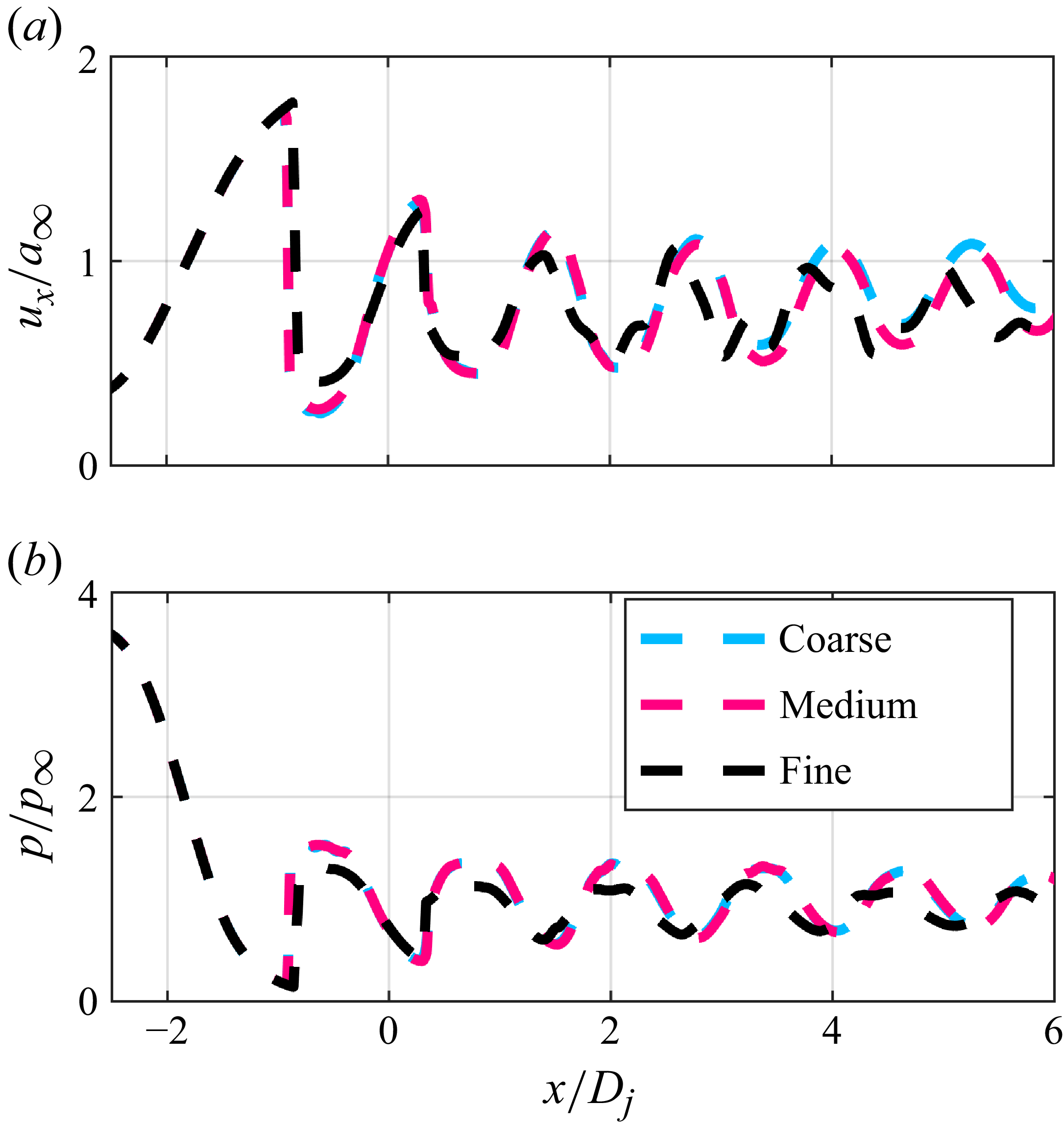
 NPR=4

 NPR=4

 NPR=4

 NPR=4
 St=0.283
 St=0.354

 NPR=4
 m=0
 St=0.354
 m=1
 St=0.283
 ϕ
 ϕ
 ϕ

 NPR=4
 m=0
 m=1

 NPR=4
 m=0
 m=1

 NPR=4
 x/Dj≈0

 x/Dj≈0
 St=0.25
 NPR=4
 m=0
 m=1

 NPR=4
 x/Dj≈0
 St=0.25
 m=0
 m=1

 NPR=4
 m=0
 m=1
 m=0
 m=1

 NPR=4
 m=1
 x/Dj=4

 NPR=4
 x/Dj=4
 m=0
 m=1

 NPR=4
 x/Dj=4
 m=0
 m=1
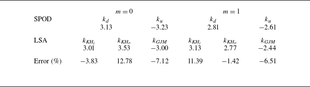

 NPR=4
 x/Dj=4
 m=0
 m=1

 NPR=4
 x/Dj=3.3
 x/Dj=[2:6]
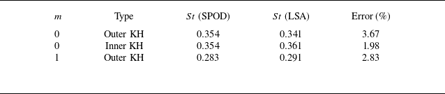
 NPR=4

 m=0
 m=1
 NPRs
 NPRs

 m=0
 m=1

 NPR=3
 NPR=4
 NPR=5

 NPR=3
 NPR=4
 NPR=5

 ksh
 NPR
 m=0
 NPR
 m=1
 NPR
 m=0
 m=1


 ϕ
 NPR=4
 m=0
 m=1

 λ
 NPR=4
 m=0
 m=1

 NPR=4

 NPR=4
 ku,min
 ku,max
 kd,min
 kd,max

 NPR=4
 m=0
 m=1

 ksh

 NPR=4
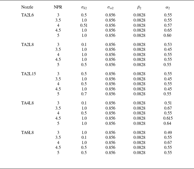
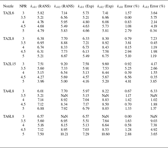
 ksh

 Open access

