


In articulating his stewardship theory of presidential power, Theodore Roosevelt emphasized that the president’s national constituency rendered the office uniquely positioned in the American political system to pursue the interests of the nation as a whole. Woodrow Wilson echoed this view. Contrasting members of Congress who are “representatives of localities” and who are “voted for only by sections of voters” with presidents who are elected by the nation, Wilson concluded that the president “is the representative of no constituency, but of the whole people.” When the president “speaks in his true character, he speaks for no special interest. If he rightly interprets the national thought and boldly insists upon it, he is irresistible” (Wilson Reference Wilson1908, 67–8).
A century later, many scholars and pundits alike continue to embrace Roosevelt’s and Wilson’s contrast between congressional parochialism and presidential universalism. For example, summarizing a mass of legal scholarship, Nzelibe (Reference Nzelibe2006, 1217) concludes: “One of the most widespread contemporary assumptions in the discourse about the separation of powers is that while the president tends to have preferences that are more national and stable in nature, Congress is perpetually prone to parochial concerns.” Political science scholarship identifies a range of factors that could encourage the president to embrace a universalistic orientation. For example, stressing norms and expectations, Cronin and Genovese (Reference Cronin and Genovese2004, 198) argues that “Once in office, presidents often bend over backward in their attempt to minimize the partisan appearance of their actions. . .Presidents are not supposed to act with their eyes on the next election; they are not supposed to favor any particular group or party.”Footnote 1
Others acknowledge that presidents, like members of Congress, pursue their political interests, such as reelection, but contend that the president’s national constituency incentivizes universalism. Subscribing to what Wood (Reference Wood2009, 19) labels a “centrist view of representation,” some scholarship argues that electoral pressures encourage presidents to respond not to specific geographic constituencies, but to the national median voter. This vision of presidential universalism contrasted with congressional parochialism remains a motivating assumption of many formal models within separation of powers scholarship. For example, game theoretic research by Howell, Jackman, and Rogowski (Reference Howell, Jackman and Rogowski2013, 3132) posits that “presidents focus on the national implications of public policies while members of Congress monitor the effects of public policy on both the nation as a whole and their local constituencies.”Footnote 2
We argue that while the universalistic framework undoubtedly captures important differences between presidents and legislators, it misconstrues the forces driving presidential behavior. We argue that presidents face strong incentives to be particularistic: that is to prioritize the needs and desires of some citizens over others when pursuing their policy agendas. We test the explanatory power of universalism versus particularism in the context of divide-the-dollar politics. Universalism suggests that presidents will pursue budgetary policies that allocate federal spending to constituencies in a manner that is unrelated to their political characteristics; maximum efficiency and appealing to the national median voter is the president’s primary objective.Footnote 3
Conversely, particularistic presidents geographically target federal spending to serve a number of ends. To maximize their prospects of reelection, presidents do not simply pursue nationally optimal outcomes or follow the preferences of the national median voter, as much universalistic scholarship argues. While the president has a national constituency, not all voters have equal influence in presidential elections; therefore presidents have incentives to respond disproportionately to the interests of Americans in constituencies with the most clout in the next presidential contest. Presidents also diverge from the norms of universalism to serve other goals. Building on research emphasizing the president’s role as a partisan leader (Cameron Reference Cameron2002; Galvin Reference Galvin2009; Milkis, Rhodes, and Charnock Reference Milkis, Rhodes and Charnock2012; Wood Reference Wood2009), we show that presidents systematically reward constituencies that reliably vote for them and their party with disproportionate shares of federal largesse. Moreover, as Berry, Burden, and Howell (Reference Berry, Burden and Howell2010) argues, presidents can also strategically allocate funds to gain leverage vis-à-vis co-partisan members of the legislature. In stark contrast to the universalistic paradigm, which paints a picture of presidents providing a counterbalance to congressional parochial impulses, we reveal substantial presidentially induced inequalities favoring politically significant constituencies.
PRESIDENTIAL CAPACITY FOR TARGETED BUDGETING
In search of Republican votes to free the Civil Rights Act of 1964 from the iron grasp of Rules Committee Chairman Howard Smith, Lyndon Johnson sought to direct a series of federal grants to Minority Leader Charlie Halleck’s district. Toward this end, Johnson reached out to NASA administrator James Webb, who had previously served as head of the Bureau of the Budget under Truman, to inquire what the agency could do for Halleck and his constituents. Three days later, Webb met with Halleck and discussed a number of research grants that could be awarded to Purdue University, which sat in Halleck’s second congressional district of Indiana.Footnote 4
Such instances of direct presidential involvement in shaping precisely where and how federal dollars are spent often go undocumented, making it difficult to assess how frequent or rare they are. But can presidents, through other mechanisms requiring less personal involvement, systematically influence the geographic allocation of federal grants in ways that serve their political needs? Since the Budget and Accounting Act of 1921, presidents have enjoyed considerable influence over the budgetary process (Bertelli and Grose Reference Bertelli and Grose2009; Larcinese, Rizzo, and Testa Reference Larcinese, Rizzo and Testa2006), and scholars have long shown how presidents use their sway over the budget to shape policy implementation (e.g., Carpenter Reference Carpenter1996; Wood and Waterman Reference Wood and Waterman1994). As Berry, Burden, and Howell (Reference Berry, Burden and Howell2010) notes, presidents have multiple opportunities to shape budgetary outcomes at both the proposal and implementation stages. In some budgetary decisions, such as those regarding natural disaster relief, presidents may have unilateral control over decisions about the allocation of funds (Reeves Reference Reeves2011). However, in most programs the primary mechanism through which presidents exercise control is through the politicization of the federal bureaucracy (Moe Reference Moe, Chubb and Peterson1985a). Specifically, by appointing like-minded officials to the top levels of management at the departments and agencies charged with crafting budgetary requests and within the Office of Management and Budget, which coordinates and oversees the process, presidents empower officials who share their political outlook to pursue budgetary allocations that fit the administration’s political needs.
Opportunities for executive branch influence emerge at the beginning of the budgetary process. The distributive politics literature has long emphasized that the power to offer the initial proposal gives an actor disproportionate influence over spending outcomes; indeed, this is the foundation of studies asserting the disproportionate influence that substantive committees wield over the allocation of federal largesse within their purview.Footnote 5 Yet, the power of proposal rests not with congressional committees, but with the White House. Since 1921, the Budget and Accounting Act has charged the president with preparing and submitting to Congress an annual budget proposal. In practice, of course, presidents do not produce draft budgets; agency officials from across the federal bureaucracy do. The preferences of key officials in the agencies formulating budgetary requests may at times diverge from those of the president, and some agencies go to great lengths to gain and protect their autonomy (inter alia Carpenter Reference Carpenter2001). However, presidents enjoy a number of tools, foremost among them the capacity to populate the bureaucracy with political appointees who share the same basic political interests, through which presidents can exercise considerable bureaucratic and administrative control over policymaking (Dickinson Reference Dickinson2005; Howell and Lewis Reference Howell and Lewis2002; Lewis Reference Lewis2003; Moe Reference Moe1985b; Rudalevige Reference Rudalevige2002; Waterman Reference Waterman1989; Hudak and Stack Reference Hudak and Stack2013).
The contemporary bureaucracy houses thousands of political appointees, including approximately 1,500 who are appointed by the president and confirmed by the Senate and another roughly 1,500 Schedule C appointees who are de facto chosen by the president with no congressional input or review (Lewis Reference Lewis2008). These appointees, quite logically, tend to share closely the ideological orientation and programmatic vision of the president they serve.Footnote 6 As a result, by filling key posts with political loyalists, presidents can create an institutional structure that increases the probability that the budget recommendations that emerge from the bureaucracy will hew closely to the White House’s own preferences and political imperatives.
Moreover, presidents have centralized considerable budgetary power within the Office of Management and Budget (OMB), which is firmly lodged in the Executive Office of the President, to protect and advance the administration’s priorities. Since the 1970s, many scholars have bemoaned the loss of “neutral competence” in OMB and the politicization of the office that has rendered it more attuned to the political needs of the president (Heclo Reference Heclo1975; House Reference House1995; Tomkin Reference Tomkin1998). At the heart of this transformation lies the increased power of political appointees versus careerists within the office. As Lewis (Reference Lewis2008, 35–6) notes, one of the key elements of the 1970 reorganization of the Bureau of the Budget into the OMB was the creation of new political appointees, most importantly four program associate directors. This created a second layer of politically appointed staff at the top of the examining divisions, which play a powerful role in shaping budgetary requests. Political appointees have only grown in number and influence over the intervening decades.
OMB plays an important role in shaping budgetary outcomes even before the departments and agencies begin to act. The process begins with OMB submitting planning guidance to executive agencies that shape their own requests. Moreover, after the agencies’ initial proposals are complete, they are submitted to OMB for a thorough review to insure that agency priorities accord with the program of the president. Taken together, the resulting process of formulating a presidential budget is stacked to create a document that reflects the president’s priorities and needs. Of course, congressional leaders may have very different budgetary priorities and the final budget need not reflect the president’s wishes. Nevertheless, the ability to set the agenda by providing the starting point for legislative debate is an important advantage. As Schick (Reference Schick2000, 109) argues, “Even when the president’s budget is reputed to be dead on arrival, the president sets the agenda for the bargaining and legislative actions that follow.”Footnote 7
Presidents also have a significant capacity to shape how federal dollars are ultimately allocated even after they are appropriated (Berry, Burden, and Howell Reference Berry, Burden and Howell2010; Gordon Reference Gordon2011). While Congress may determine the amount of money allocated to a specific department or agency, the bureaucracy itself often wields considerable influence through a variety of mechanisms over how such funds are ultimately distributed. In his seminal analysis, Arnold (Reference Arnold1979, 8) notes that “most decisions about geographic allocation are bureaucratic decisions.” Here, again, by installing men and women who share the White House’s priorities in positions of leadership throughout the bureaucracy, presidents stack the deck in their favor and raise the odds that policy as implemented will reflect their preferences and political imperatives to the greatest extent possible.Footnote 8
Thus, through politicization of the departments and agencies, the empowerment of a responsive OMB, and through occasional direct presidential involvement, presidents may wield considerable influence over budgetary policymaking at the agenda-setting stage, during the course of the legislative debate, and during policy implementation. Presidents possess the institutional capacity to act on particularistic motives.Footnote 9 With this in mind, we consider three forms of particularism that might influence presidential behavior.Footnote 10
ELECTORAL PARTICULARISM
First, we argue that presidents engage in electoral particularism. While acknowledging that members of Congress possess multiple goals, most congressional scholarship has long given preeminence to electoral incentives in driving particularistic behavior in Congress (Mayhew Reference Mayhew1974). Presidency scholarship has accorded varying levels of importance to the electoral connection. One branch of scholarship, exemplified by works like Moe and Wilson (Reference Moe and Wilson1994) and Howell and Brent (Reference Howell and Brent2013), argues that presidents, in stark contrast to members of Congress, care relatively little about reelection. This enables presidents to pursue their policy preferences and historical legacies relatively unencumbered by electoral concerns: “His large, heterogeneous, competitive constituency, along with the lower priority accorded to reelection, gives him substantial freedom to pursue his own distinctive vision of the public agenda” (Moe Reference Moe1990, 237). If correct, presidents should have scant incentives to engage in parochial politics, an inefficient targeting of federal dollars to key constituencies for electoral gain.
Other scholars have argued that presidents are driven by multiple goals, including historical achievement, good public policy, and reelection (e.g., Light Reference Light1998 [1982]). The advent of the permanent campaign illustrates how reelection-oriented activities have come to dominate presidents’ schedules, including how much time they spend fundraising, for themselves and their co-partisan allies, and where they travel (Doherty Reference Doherty2012; Charnock, McCann, and Tenpas Reference Charnock, McCann and Tenpas2009). Yet, these studies mostly speculate on the implications of these developments for policy outcomes. As Doherty (Reference Doherty2012, 8) notes, “Few studies have attempted to examine empirically the extent to which electoral incentives relate to the ways sitting presidents govern.”Footnote 11
What are the implications of presidential reelection incentives for budgetary policy? One prominent view suggests that reelection incentives drive presidents away from particularism. Because voters judge presidents primarily on national conditions, such as the state of the economy, presidents should best serve their electoral prospects by pursuing policies that maximize outputs for the greatest number of people.Footnote 12 Whereas electoral incentives produce parochialism in Congress, they encourage universalism from presidents.
Canes-Wrone (Reference Canes-Wrone2006) offers a more nuanced view. Most presidents most of the time pursue their vision of good public policy that will benefit their historical legacies. However, as reelection approaches, some presidents—specifically, presidents with marginal approval ratings—will face incentives to pander to the national median voter. For these presidents, Canes-Wrone (Reference Canes-Wrone2006) finds that their budgetary requests come into greater alignment with the public’s budgetary preferences in a reelection year.Footnote 13
We focus not on whether presidential budgets match the programmatic priorities of the median voter, but on the allocation of those federal dollars across the country. Here, the median voter’s preferences are clear: the vast majority of Americans disapprove of targeted, pork-barrel spending. Whereas geographic targeting makes sense for members of Congress, an inefficient geographic targeting of federal dollars for political gain is unlikely to appeal to the national median voter.Footnote 14 Nevertheless, we argue that presidents have strong incentives to engage in precisely this sort of particularistic behavior.
Most prior studies of electoral politics privilege national factors over local forces in presidential elections. The relative weight that voters place on national versus local concerns will vary across individuals and over time; however, a growing number of studies suggest that the localized consequences of federal policies have significant and consistent impacts on presidential electoral fortunes (e.g., Books and Prysby Reference Books and Prysby1999; Gasper and Reeves Reference Gasper and Reeves2011b; Kriner and Shen Reference Kriner and Shen2007, Reference Kriner and Shen2010; Reeves Reference Reeves2011; Reeves and Gimpel Reference Reeves and Gimpel2012). Most relevant for our analysis here is Kriner and Reeves (Reference Kriner and Reeves2012), which demonstrates that voters reward presidents for the share of federal spending that their local communities receive.
A local component to presidential elections is not a sufficient incentive for presidents to engage in electoral particularism. If all voters have equal weight in selecting the next president, then the best strategy for securing the most votes is to benefit the greatest number of people. But presidential elections are determined by states casting electoral votes in an all-or-nothing manner.Footnote 15 In recent presidential elections, most states have been firmly in one partisan camp or the other. As a result, voters in a handful of swing states are plainly of much greater electoral importance to the president than voters in electorally uncompetitive states. Campaign scholars have long noted that the institutional design of presidential elections compels candidates to concentrate their resources on contacting and persuading voters in swing states at the expense of the majority of voters in the rest of the country (e.g., Banzhaff Reference Banzhaff, III1968; Bartels Reference Bartels1985; Brams and Davis Reference Brams and Davis1974; Nagler and Leighley Reference Nagler and Leighley1992; Shaw Reference Shaw2006). We argue that it also has tangible and substantively meaningful implications for federal budgetary policymaking. Rather than embracing universalism, presidents have incentives to engage in their own brand of particularism (Hudak Reference Hudak2014). The electoral system provides a president with strong incentives to target federal grant dollars to localities within swing states in the hopes of maximizing his and his co-partisan successor’s chances of winning the next election.Footnote 16
If presidents are driven by electoral incentives to systematically target federal dollars to swing states, then the incentives for swing state targeting should vary with the electoral calendar. Political scientists have long searched for evidence of a “political business cycle” in presidential politics (e.g., Alesina, Roubini, and Cohen Reference Alesina, Roubini and Cohen1997; Tufte Reference Tufte1978). Numerous studies suggest that voters have remarkably short memories. For example, in an analysis of decades of data on voting behavior, Bartels (Reference Bartels2008) finds evidence of “myopic voters” who fail to consider economic performance over the course of an entire presidential term and instead respond to only the most recent changes in the state of the economy.Footnote 17 Voters prioritize actions and developments that happened recently and discount developments that happened in the more distant past (Healy and Lenz Reference Healy and Lenz2014; Huber, Hill, and Lenz Reference Huber, Hill and Lenz2012). Furthermore, Bartels (Reference Bartels2008) suggests that presidents may manipulate elections by pursuing policies that produce short-term economic benefits in the run-up to an election that will distract voters from poor economic stewardship in prior years.
This suggests that presidents stand to gain the greatest electoral advantage from targeting federal dollars to swing states in the immediate lead-up to an election. If electoral incentives drive swing state targeting, we expect swing state targeting to be concentrated in election years. Additionally, we hypothesize that the electoral incentive for swing state targeting should be strongest when the president himself is set to face the voters in a reelection battle. A term-limited president is still incentivized to help his party’s reelection chances to boost the prospects of a co-partisan successor in order to defend their policy legacies from incursions and reversals by a new president of the opposition party. Still, the incentive to stay in office is likely even stronger.
Finally, by examining where within swing states presidents target federal grants, we can offer fresh insight into a debate within the campaigns literature. Most states are large, heterogeneous constituencies that offer diverse electoral landscapes. If a president wants to maximize his chances of winning a state by using all available levers to influence budgetary policy, how should he proceed? Does an additional grant dollar have the same influence on the likelihood of winning the election, regardless of where in the state it is spent?
Scholars have long argued over the relative explanatory power of the core voter (Cox and McCubbins Reference Cox and McCubbins1986) and swing voter (Lindbeck and Weibull Reference Lindbeck and Weibull1987) models.Footnote 18 The former posits that the most efficient way to maximize votes is for a political actor to allocate distributive benefits, like federal grants, to constituencies in which they previously enjoyed considerable electoral support. For risk-averse politicians, the optimal strategy is to use targeted spending to shore up support among loyal voters and solidify the political base of their reelection coalition. By contrast, the latter model outlines the logic for targeting swing voters. While both models have merit, Cox (Reference Cox, Shapiro, Stokes, Wood and Kirshner2010) argues that expanding the scope of the formal models to focus on the capacity of resource targeting not only to persuade voters, but also to improve coordination and mobilization, tilts the balance decisively toward the core voter model. If this perspective is correct, then we should see evidence of presidents targeting federal grants disproportionately to core constituencies within swing states. That is, presidents should gain maximum advantage from targeting grant dollars to strongly co-partisan counties with a track record of voting for the president’s party that reside within swing states that are in play in the upcoming presidential election.
Partisan Particularism
Second, we consider partisan particularism. Presidents may target based on criteria other than electoral competitiveness. Presidency scholars, perhaps reflecting the Founders’ own ambivalence toward political parties, have long been wary of conceptualizing presidents as party leaders. For example, Pious (Reference Pious1996, 18) argues that “in the final analysis, the president is of the party—but also above it and sometimes in opposition to it. He or she does not find it of any great use to attempt to be a strong party leader.” Yet, recent scholarship has challenged this perspective noting that contemporary presidents are undeniably the leaders of their political party who face pressure to reward their partisan supporters and solidify their base of support. For example, Wood (Reference Wood2009, 36) argues that presidents “are driven more by partisanship than by a thirst to reflect the larger preferences of the community.” This partisan dynamic may also encourage presidents to weigh the well-being of some voters over that of others and to prioritize the interests of some constituencies over those of the nation as a whole.
By pursuing programmatic agendas and budgetary policies that disproportionately benefit co-partisans, a new form of geographic inequity in the allocation of federal benefits may arise. Rather than federal dollars being targeted only to swing states, constituencies that are highly populated with presidential co-partisans—which we label “core states”—should also reap disproportionate shares of federal benefits.Footnote 19 This advantage may be even greater in core counties within core states—the strongest bastions of presidential party strength.
A focus on the political business cycle also affords insights into the mechanisms driving core state targeting. Some have argued that presidents could engage in core state targeting to pursue electoral aims. This is because core states represent a “safer investment,” and “risk-averse political actors who want to maximize their chances of winning elections should allocate more funds to loyal states” (Larcinese, Rizzo, and Testa Reference Larcinese, Rizzo and Testa2006).Footnote 20 Alternatively core state targeting might occur because of a president’s programmatic agenda. By implementing policies supported by partisan supporters, he may direct money to locales where his supporters are concentrated and away from enclaves of opposition voters.Footnote 21 If counties in core states see more money in election years, this suggests an electoral mechanism. To the extent that core targeting is present equally in election and nonelection years, the data would be more consistent with a programmatic mechanism through which presidents seek to benefit key components of their core partisan constituency.
COALITIONAL PARTICULARISM
Third, we consider coalitional particularism. A desire for greater influence vis-à-vis the legislature can induce presidents to target benefits to parts of the country that elect co-partisans to Congress. In a seminal analysis of presidential targeting, Berry, Burden, and Howell (Reference Berry, Burden and Howell2010) argues that presidents use the various tools at their disposal to pursue budgetary policies that concentrate federal dollars in constituencies represented by their fellow partisans in Congress.Footnote 22 Targeting grant dollars to the constituencies of co-partisan members can serve a number of goals. First, contemporary presidents are expected to be partisans in chief. Shifting more federal resources toward co-partisan members helps satisfy partisan demands. Second, co-partisan targeting provides presidents with valuable political currency on Capitol Hill. Members of Congress highly value specific federal benefits like grants for their districts. By helping co-partisans procure them, presidents seek to win political favors that they can call upon for support of their major priorities. Indeed, solidifying support among their co-partisans on Capitol Hill has long been recognized as a key legislative coalition building strategy (Cohen Reference Cohen2006; Edwards Reference Edwards, III2000). Third, presidents may target federal dollars to co-partisan members’ constituencies with an eye toward the future in the hopes of bolstering their party’s ranks in succeeding Congresses. While political pundits often emphasize various sources of presidential power, like the president’s eloquence, his arm twisting ability in private negotiations, or his standing among the public, decades of research has consistently shown that the strength of the president’s party in the legislature is the most important factor influencing the president’s success in Congress.Footnote 23 As a result, through this type of particularistic targeting, presidents can pursue a mix of partisan and legislative goals.
DATA AND METHODS
To what extent do presidents influence the distribution of federal grants across geographic constituencies in the United States? To answer this question, we follow Berry, Burden, and Howell (Reference Berry, Burden and Howell2010) and Kriner and Reeves (Reference Kriner and Reeves2012) and compile data from the Consolidated Federal Funds Report (CFFR) on every federal grant program from 1984 to 2008.Footnote 24 For each program, the CFFR reports the amount of money spent in each county in a given year.
From 1984 to 2008, following a general increase in overall government spending, the total amount that the median county received gradually rose from just over eleven million dollars in 1984 to nearly forty million dollars in 2008. Grants accounted for between 10.3% and 14.6% of all federal spending reported in the CFFR during this time.Footnote 25 Following Berry, Burden, and Howell (Reference Berry, Burden and Howell2010), we construct our dependent variable as the amount of grants received by a county in a year. We take the natural log to ensure that our results are not skewed by outlying values, and after taking the logarithmic transformation, our dependent variable is approximately normally distributed, as shown in the Supporting Information.Footnote 26
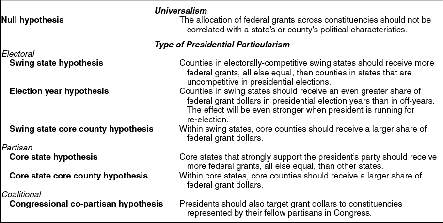
Table 1 summarizes the main empirical predictions of the universalistic presidency framework and our contrasting arguments for presidential particularism. If presidents do indeed strictly pursue the national interest and maximally efficient policy outcomes, then the share of federal grant dollars that a county receives should be unrelated to its political characteristics. However, if electoral, partisan, and coalition incentives encourage presidents to deviate from the norms of universalism, then presidents should seek to target federal dollars to politically valuable constituencies.
Summary of Hypotheses

Assessing Presidential Particularism
We hypothesized that presidents have strong incentives to target federal resources disproportionately to states that are likely to be the most competitive in the next electoral contest. By contrast, the null hypothesis generated by the universalistic presidency view contends that swing states will not receive any more federal grant dollars than nonswing states, all else being equal. We measure electoral competitiveness as the average share of the two party vote that the losing candidate received over the three preceding presidential elections. We identify swing states as those in which the losing candidate averaged 45% or more of the two-party vote over the past three election cycles.Footnote 27 Though our results are robust to continuous specifications of the competitiveness variable, which we include in the Supporting Information, we utilize these categories since they reflect the way most campaigns view the competitiveness of states (Shaw Reference Shaw2006).
To assess the core state hypothesis, we include a similar measure identifying counties that reside in states solidly in the president’s column. A county is in a core state if the president’s party averaged 55% or more of the two-party vote in that state in the preceding three elections. If presidents systematically pursue policies that reward their co-partisans, then we should also observe counties in core states receiving a disproportionate share of federal dollars.Footnote 28 Finally, to test an alternative form of presidential particularism suggested by Berry, Burden, and Howell (Reference Berry, Burden and Howell2010), we include a dummy variable coded 1 if a county is represented in the House by a member of the president’s party.Footnote 29
Given the central role that Congress plays in budgetary politics, to model the level of federal spending that a county receives we must also control for the characteristics of that county’s representative in Congress. Existing scholarship offers two main hypotheses concerning the specific types of members who will be able to secure more federal dollars for their districts. First, studies have argued that members of the majority party in Congress will seize a disproportionate share of federal dollars (inter alia Albouy Reference Albouy2013; Balla et al. Reference Balla, Lawrence, Maltzman and Sigelman2002; Cox and McCubbins Reference Cox and McCubbins2007; Levitt and Sndyer Reference Levitt and Sndyer1995; Martin Reference Martin2003). Legislative scholars have long noted the institutional advantages that members of the majority party enjoy, particularly in the House. Majority members enjoy greater powers of proposal; they largely determine what legislation the chamber will consider, and this power to set the legislative table affords considerable influence (e.g., Cox and McCubbins Reference Cox and McCubbins1993). The majority party also can influence the agenda and keep competing proposals that are less advantageous to their members off the agenda (Albouy Reference Albouy2013; Campbell, Cox, and McCubbins Reference Campbell, Cox and McCubbins2002; Den Hartog and Monroe Reference Den Hartog and Monroe2011; Gailmard and Jenkins Reference Gailmard and Jenkins2007; Lee Reference Lee2009). Thus, to account for the power of the majority party over the allocation of federal dollars, our analysis assesses the influence of whether a county’s representative is a member of the majority party in the House on the share of federal grants that it receives. If the majority party is able to use its various levers of influence to skew federal dollars toward its members’ districts, then we would expect counties represented by majority party members to receive, on average, more federal grants than counties represented by members of the opposition.
Other scholars of budgetary outcomes focus on congressional committees. Distributive models of Congress emphasize the role of committees in directing federal dollars back to members’ districts (e.g., Adler and Lapinski Reference Adler and Lapinski1997; Deering and Smith Reference Deering and Smith1997; Shepsle and Weingast Reference Shepsle and Weingast1981, Reference Shepsle and Weingast1987). For this reason, we include controls for whether a locality is represented by a committee chair or a member of the Ways and Means or Appropriations Committees, which hold direct jurisdiction over all legislation involving revenue and over the appropriations process itself.Footnote 30
Finally, we include several demographic control variables. Most importantly, we control for each county’s population in each year.Footnote 31 We also include two controls for a county’s socioeconomics: per capita income in constant 2008 dollars and the poverty rate.Footnote 32 Both may be positively correlated with federal spending. Counties with high per capita incomes may have greater demand for federal grant programs. Counties with high poverty rates have a greater need for federal assistance.
RESULTS
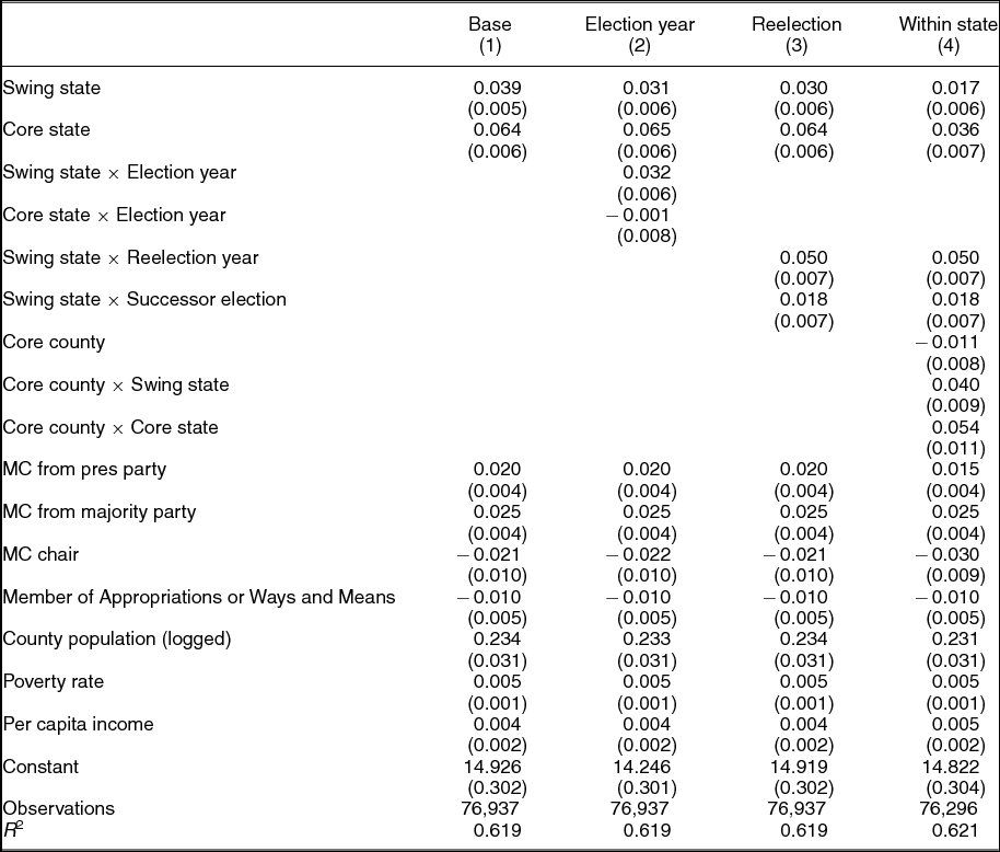
We estimate least-squares regression models that include both county and year fixed effects and report standard errors clustered on the county. The inclusion of county fixed effects allows us to assess the influence of electoral competitiveness controlling for all time-invariant county characteristics—both observed and unobserved. The inclusion of year fixed effects controls for national swings from contest to contest. Table 2 presents the results.
Presidential Particularism and the Allocation of Federal Grants, U.S. counties, 1984 to 2008

Notes: Robust standard errors clustered on county in parentheses. Least-squares model with fixed effects for counties and years. Dependent variable is the natural log of federal grant spending in each county in a given year.
As shown in the model presented in column 1, we find strong evidence of presidential particularism with support for our swing state, core state, and co-partisan congressional hypotheses. The coefficients for these variables are all positive and statistically significant. These findings are inconsistent with the universalistic presidency model, which contends that the allocation of federal funds should not be related to political variables. Even in budgetary policymaking—a context where the president’s authority is checked by many other actors—we see strong evidence of presidential particularism as constituencies of greater political importance to the president secure significantly greater shares of federal dollars than other constituencies. These relationships are robust across multiple specifications.Footnote 33
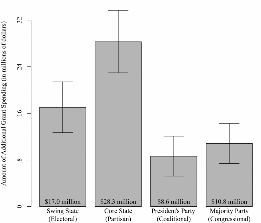
How much money is in play? To provide further context for the findings in column 1 of Table 2, consider that in 2008 the population-weighted median county received $428 million in federal grant aid.Footnote 34 To illustrate the estimated relationship between federal funding and various forms of particularism, Figure 1 presents the additional funds that the median county would receive if it was located in a swing state or core state, or if it was represented by a member of the president’s party or of the majority party in the House.Footnote 35 In 2008, this means that the median county in a swing state received $17 million more in grant spending than did an identical county in an electorally uncompetitive state, all else being equal.Footnote 36 This swing state bonus in grant spending can prove a significant windfall for a county; the additional funds could hire dozens of police officers or teachers, improve key stretches of road in bad repair, or expand a government-subsidized daycare program that helps many transition from welfare to work.
Presidential Particularism and Federal Grant Spending (county-level effects)

This is strongly consistent with our argument that presidents engage in particularism to bolster their and their party’s prospects at the next election. While we cannot conclusively determine from observational data that greater shares of spending allocated to swing states are the result of presidential targeting, it bears repeating that presidents and their co-partisan successors are the only obvious beneficiaries of swing state targeting. Members of Congress have little incentive to use their powers as appropriators to disproportionately channel funds to voters in presidential swing states. Rather, the advantage these counties enjoy serves only the interest of the president.
We also find strong evidence that presidents engage in another form of particularism; that is, they pursue budgetary policies that also disproportionately advantage counties located in core states that solidly backed the president’s party in recent elections. The median county in a core state was rewarded for its loyalty at the ballot box with $28.3 million more in grant funding, on average, than a similar county in a noncore state. This is further evidence of presidential particularism. Rather than pursuing policies that do not discriminate between beneficiaries on the basis of their political characteristics, the data suggest that presidents pursue budgetary policies that channel federal grant dollars systematically toward core partisan constituencies. All else being equal, counties in states that strongly voted for the president in recent elections reaped a disproportionate share of federal dollars.
Consistent with prior research (Berry, Burden, and Howell Reference Berry, Burden and Howell2010), we also find evidence of the congressional co-partisan hypothesis. Presidents target federal grant dollars to counties represented by a co-partisan member of the House. However, the boost in spending that such counties enjoy—approximately $8.6 million in the median county—is substantially less than the amounts received by counties in swing or core states.
Our results also present evidence of congressional particularism. After all, for decades political scientists have documented the pressures members feel to bring home targeted benefits for their constituents to bolster their hopes of reelection. Indeed, the image of the pork-barreling legislator is burned into our national consciousness; we expect congressional budgeting to be characterized by rampant parochialism. Yet, the evidence for it is surprisingly modest. Counties represented by the majority party in the House receive only about 2.5% more grant spending, on average, than counties represented by the minority party. Moreover, we found no evidence that counties represented by committee chairs or members of the Appropriations or Ways and Means Committees enjoyed any more benefits, on average, than those represented by rank and file members.
Thus, surprisingly our data suggest that presidential particularism is an even greater source of inequality in the distribution of federal grants across the country than congressional particularism. That is not to say that budgetary politics would necessarily be more efficient if Congress alone made decisions concerning how federal dollars are spent across the country. Indeed, there are good reasons to think it would not be so. However, it does suggest that a county’s political importance to the president—whether it is in a swing or core state—is more important than the characteristics of that county’s representative in Congress in determining the share of federal spending it receives.
Election Year Targeting
To test our hypotheses concerning swing and core state targeting and the political business cycle, Table 2 column 2 includes the interactions of the swing and core state variables with an election year indicator. We find that swing state targeting is especially acute during election years as presidents target myopic voters in swing states for electoral gain. By contrast, core state targeting does not vary with the electoral cycle.
The coefficient for the main effect for the swing state variable is positive and statistically significant, though smaller than in the base model in column 1.Footnote 37 Swing states receive some boost in federal grant spending in all years. However, strongly consistent with our argument, the election year interaction is also positive and significant—in other words, the swing state advantage increases significantly in the immediate lead up to a presidential election.
For core states, by contrast, we do not see any variation in the size of the effect with the electoral calendar. The core state coefficient is again positive and statistically significant. However, the election year interaction is substantively small and not statistically significant. This suggests that core state targeting is not a function of electoral considerations. Rather, presidents consistently pursue budgetary allocations that disproportionately benefit their partisan base.
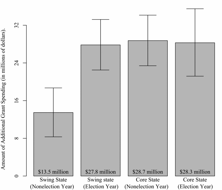
As with the previous figure, Figure 2 presents estimates of the substantive effects (derived from column 2 in Table 2) of swing state and core state targeting on grant spending in the population-weighted median county. Counties in swing states always receive a disproportionately large share of federal grants. In nonelection years, the median county in a swing state receives approximately $13.5 million more than the median county in an electorally uncompetitive state, all else being equal. However, strongly consistent with our theory, we find that this swing state advantage increases significantly during election years. Because voters reward presidents only for the most recent policy developments, the electoral incentive to target federal dollars to swing states are strongest in the immediate run up to the election. As a result, during election years counties in swing states receive twice as much additional federal grant funding as they do in nonelection years. In election years, the median county in a swing state receives $27.8 million or fully 6.5% more federal grant dollars than a similar county in a nonswing state.
Presidential Particularism and the Political Business Cycle (county-level effects)

We also continue to find strong evidence that presidents target federal grants to core states; however, this dynamic does not vary with the electoral calendar. Counties in core states always receive more grant dollars, on average, than counties in noncore, nonswing states, regardless of whether it is a presidential election year. This suggests that presidents do not primarily target grant dollars to core constituencies for electoral purposes. If shoring up the partisan base was the primary aim, then core state targeting should also increase in election years. Rather, the consistency of core state targeting over time is more consistent with a programmatic mechanism through which presidents reliably channel federal benefits disproportionately to core co-partisan constituencies.
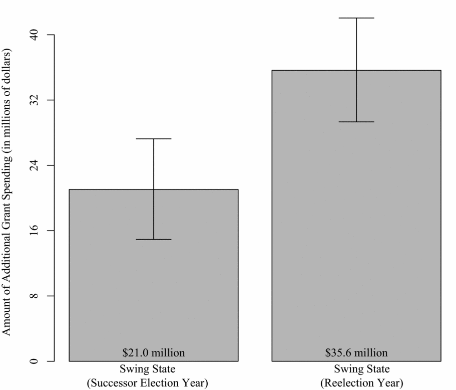
The second component of our electoral cycle hypothesis was an expectation that the effect would be strongest when the president himself is seeking reelection. Of the seven elections in our data set, four (1984, 1992, 1996, and 2004) were reelection contests; three (1988, 2000, and 2008) were open seat races. If the swing state advantage is the result of presidential targeting for electoral gain, then swing states should reap the greatest rewards in presidential reelection years. Though presidents face strong incentives to elect co-partisan successors, the drive for reelection is likely even stronger. Column 3 in Table 2 presents this analysis by including an interaction between the swing state variable and a dummy variable identifying reelection years, as well as an interaction between the swing state variable and a dummy variable identifying open seat election years. The main effect for swing states remains positive and statistically significant. Swing states always receive a disproportionate share of federal grant dollars. The coefficient for the swing state × successor election interaction variable is also positive and statistically significant. Swing states receive an even larger share of grants, on average, in election years, even when the sitting president is not on the ballot. Finally, and strongly consistent with the logic of our theory of electorally induced particularism, the coefficient on the swing state × reelection year interaction is also positive, substantively large, and statistically significant. Wald tests show that the coefficient for the reelection year interaction is significantly greater than the coefficient for the successor election year interaction, p < .01. The regression results suggest that a county in a swing state in a presidential reelection year receives 8% more federal grant dollars than an identical county in a nonswing state, all else being equal. As shown in Figure 3, for the median county in 2008 this would translate into a $35.6 million infusion of federal largesse.
Presidential Particularism, and Presidential Incumbency (county-level effects)

Targeting within States
Finally, we examine whether presidents target grants to certain types of counties within swing and core states. This model is presented in column 4 of Table 2, and includes three new variables: an indicator for core counties, defined as those in which the president’s party averaged 55% or more of the two party vote in the preceding three elections, and the interactions of this variable with both the swing and core state indicator variables. Figure 4 provides a substantive interpretation of the main results for the median county.
Presidential Particularism Within-States (county-level effects)

Consistent with Cox (Reference Cox, Shapiro, Stokes, Wood and Kirshner2010), we find evidence that presidents do not target money indiscriminately within swing states. Rather, presidents send money disproportionately to core constituencies within swing states. The relevant coefficient is positive and statistically significant. As shown in Figure 4, our model estimates that the median core county in a swing state receives almost $12.6 million more in federal grants than a noncore county within the very same state.
We also find strong evidence that presidents reward the strongest component of their partisan constituency: core counties within core states. Core counties received approximately 4% more in grant spending than noncore counties located within the same core state. This suggests the median core county in 2008 would have received roughly $18.8 million more in grant spending than another county in the same core state that did not reliably back the president’s party, all else being equal. Only core counties in states that reliably backed the opposition party at the polls did not receive an infusion of federal grant dollars.
Thus, the evidence for presidentially induced inequality in budgetary outcomes is both wide and deep. Presidents do not simply pursue policies that benefit all Americans equally; rather, they champion budgetary policies that channel federal dollars disproportionately to states and communities that are critical to their and their party’s electoral fortunes, as well as to those that are dominated by their co-partisans in the mass public.
DISCUSSION
Our county-level analysis of federal spending from 1984 to 2008 marshals a wealth of data and examines three broad types of presidential particularism. We further consider how electoral cycles and county-level characteristics influence targeting. We find strong and consistent evidence that presidents are not universalistic, but particularistic: they target federal grants to pursue reelection, reward their partisan base, and bolster their legislative coalition in Congress.
Most presidential scholarship has either downplayed the importance of the electoral connection, or argued that it leads presidents to pander to the median voter. By contrast, we find that the desire for reelection encourages presidents to engage in decidedly parochial politics. Election-year allocations of federal grants would be the envy of any campaign manager. In election years, swing state counties that are supportive of the president see billions of dollars more in federal spending just by virtue of the state in which they are located. The logic underlying this behavior is grounded in recent scholarship showing that voters hold presidents accountable for the share of federal dollars their localities receive and reward presidents for such efforts.
We also find strong evidence that presidents exert significant influence over the budgetary process to channel federal dollars disproportionately to strongly co-partisan counties and states. Rather than catering to the preferences of the national median voter, presidents pursue budgetary policies that systematically advantage their core partisan base. This core constituency targeting does not appear to be motivated by electoral concerns; rather the inequality persists regardless of the electoral calendar. What motivates this consistent and significant geographic inequality in federal funding? We suggest two possibilities. First, such inequalities may be the result of presidents pursuing universalistic ends through particularistic means. For example, a Democratic president may firmly believe that the national interest is best served by closing the education gap between rich and poor communities through increased federal funding for schools in urban and socioeconomically disadvantaged districts. The result is that poor, urban districts that exhibit the most need and also happen to be staunchly Democratic receive the most money.Footnote 38
However, our evidence of core state targeting also supports an alternative interpretation in which presidents are not national leaders, but rather predominantly leaders of the partisan coalitions that elected them to office. Wood’s partisan theory of presidential representation posits: “Having achieved electoral success, presidents are anxious to pursue their most favored policies and reward core supporters with benefits that accrue from election outcomes. . . .Given these partisan incentives, after elections presidents respond whenever possible to ideological imperatives and pursue partisan principles that reflect their own vision of the larger interests of the community” (Wood Reference Wood2009, 36).Footnote 39 Presidents and their appointees throughout the executive branch place their thumbs on the scales of policymaking to advantage co-partisan constituencies.Footnote 40 Presidents act in the same way as Congress scholars have long argued the majority party in Congress approaches budgetary policymaking; they simply prove far more effective at skewing outcomes toward their co-partisans’ advantage. From observational data alone we are unable to determine conclusively which of these two underlying motivations is producing the geographic inequalities we see. However, the data is strongly consistent with claims that presidents privilege their partisan priorities.
Presidential particularism may be an even more prominent feature of American politics today than in the past. Because a comprehensive county-level account of federal spending begins only in the early 1980s, we lack the requisite data to determine definitively whether presidents aggressively pursued particularistic budgetary policies in earlier eras. However, the electoral, partisan, and coalitional incentives driving particularism are likely stronger today than in the recent past. The average margin of victory in the Electoral College has fallen precipitously since the 1980s.Footnote 41 As a result, the temptation to engage in swing state targeting should be stronger for current than past presidents. Increasing partisan polarization is the most oft-discussed feature of the contemporary Congress; but as the parties have polarized the demands for presidents to serve as partisan leaders have also increased considerably. Forced to rely on near-unanimous support from co-partisans, the incentives to maintain the core of their legislative coalition have also strengthened in recent decades.Footnote 42
Finally, our findings also highlight the perils of taking the assumptions of universalism too far. For instance, universalistic claims underlie a growing chorus of scholarly calls for increased delegation to the executive branch as a solution to our contemporary political malaise. Many legal scholars have argued that greater congressional delegation to the executive yields more normatively desirable policy outcomes that better reflect the needs of the nation as a whole (Fitts and Inman Reference Fitts and Inman1991–1992; Kagan Reference Kagan2001; Marshaw Reference Marshaw1985). Indeed, Kagan (Reference Kagan2001, 2339) argues that our contemporary era of polarized divided government “create[s] a need for institutional reforms that will strengthen the President’s ability to provide energetic leadership in an inhospitable political environment.” Similarly, in their prescriptive analysis of contemporary politics Mann and Ornstein (Reference Mann and Ornstein2013, 166) argues “modest shifts to give more leeway to the executive make sense, given the current and continuing dysfunction.” Howell and Moe (Reference Howell and Moe2013) goes further, arguing that Congress is institutionally ill-equipped to craft efficient policy solutions to the nation’s most pressing problems; instead, they contend that expanded presidential power provides the best prospects for devising optimal solutions for the nation as a whole.
While greater delegation to the president may break Washington gridlock, we argue it will not necessarily lead to nonparochial policies that cater to the national median voter and the interests of the nation as a whole. Rather, because electoral and partisan forces combine to encourage presidents to engage in their own brand of particularism, the unequal distribution of policy benefits may simply better reflect the president’s political interests than those of members of Congress.




Comments
No Comments have been published for this article.