1 Introduction
Recent decades have seen rapid growth in our understanding of the dynamics of single-component gravity currents (Benjamin Reference Benjamin1968; Simpson Reference Simpson1999; Ungarish Reference Ungarish2009; Linden Reference Linden, Chassignet, Cenedese and Verron2012) based on laboratory experiments (Huppert & Simpson Reference Huppert and Simpson1980), field observations (Huppert (Reference Huppert2006) and references therein), high-resolution numerical simulations (Härtel, Meiburg & Necker Reference Härtel, Meiburg and Necker2000; Cantero, Balachandar & Garcia Reference Cantero, Balachandar and Garcia2007; Meiburg, Radhakrishnan & Nasr-Azadani Reference Meiburg, Radhakrishnan and Nasr-Azadani2015) and novel theoretical approaches (Borden & Meiburg Reference Borden and Meiburg2013). These investigations have elucidated the dynamical force balances governing the various stages of single-component gravity current flows, as well as their front velocity, mixing properties and energy budgets. By comparison, multicomponent gravity currents remain much less well understood, in spite of their importance in natural settings and engineering applications such as river plumes (Alavian et al. Reference Alavian, Jirka, Denton, Johnson and Stefan1992), oceanic overflows (Legg Reference Legg2012) and desalination plants (Law, Ho & Monismith Reference Law, Ho and Monismith2004). Most of the research on two-component gravity currents to date has focused on the influence of a particulate phase, and on the role of particle settling in triggering buoyancy reversal in such flows (Sparks et al. Reference Sparks, Bonnecaze, Huppert, Lister, Hallworth, Mader and Phillips1993; Meiburg & Kneller Reference Meiburg and Kneller2010). On the other hand, very few investigations have focused on the effects of double diffusion on the dynamics of gravity currents driven by temperature and salinity differences.
Double diffusion is known to give rise to a host of complex dynamical phenomena in nominally stably stratified thermohaline systems (Radko Reference Radko2013). At the most basic level, the experiments of Huppert & Turner (Reference Huppert and Turner1981) demonstrate that a fingering interface forms when the slowly diffusing component is unstably stratified, while a diffusive interface emerges for an unstable stratification of the faster diffusing component. The subsequent evolution of the convective flow can produce such interesting features as collective fingering instabilities, staircases and horizontal intrusions (Stellmach et al. Reference Stellmach, Traxler, Garaud, Brummell and Radko2011; Traxler et al. Reference Traxler, Stellmach, Garaud, Radko and Brummell2011). To date, double-diffusive convection has primarily been explored for base states in which the fluid is at rest. On the other hand, for base states in the form of gravity currents, characterized by sharp fronts, pronounced temperature and salinity gradients, as well as strong shear, we might expect the evolution of double-diffusive convection to proceed quite differently. This was confirmed in the laboratory experiments of double-diffusive gravity currents by Maxworthy (Reference Maxworthy1983), who explored the scaling laws and force balances governing both fixed volume and constant flow rate double-diffusive currents and intrusions. The experiments by Yoshida, Nagashima & Ma (Reference Yoshida, Nagashima and Ma1987), while similar in nature, focused on double-diffusive gravity currents with small density differences, and on the ways in which such currents evolve differently from their single-diffusive counterparts.
Laboratory experiments are commonly constrained by the choice of salt, sugar and heat as the diffusing scalars, so that it is difficult to explore the influence of the diffusivity ratio on double-diffusive phenomena in a systematic fashion. At the same time, it is challenging to obtain detailed time-dependent information on velocity and scalar concentration fields from laboratory experiments. Numerical simulations, on the other hand, are free to vary the diffusivity ratio within a wider range that is effectively bounded only by resolution requirements. Consequently, the present investigation focuses on exploring the interplay between gravity current flows and double diffusion, and on quantifying the dynamics of such flow fields as a function of the diffusivity and stability ratios. Section 2 will define the physical set-up, and formulate the governing equations and dimensionless parameters. Section 3 briefly reviews the computational approach, while § 4 focuses on the simulation results. It discusses the dependence of the gravity current velocity and thickness on the governing parameters, as well as the structure of the resulting density and velocity fields. The convective and diffusive fluxes of heat and salinity out of the current will be quantified, along with the various components of the energy budget. In order to estimate the turbulent drag acting on the current, and its role in the overall force balance, we will analyse the momentum flux across the current/ambient interface. Some interesting aspects will be highlighted regarding the late-stage dynamics of double-diffusive gravity currents. Section 5 provides information on the force balances governing double-diffusive gravity currents, while § 6 compares the results of two- and three-dimensional simulations. Lastly, § 7 summarizes the findings of the present study.
2 Physical problem
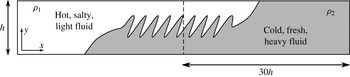
We perform direct numerical simulations of full depth, double-diffusive lock-exchange gravity currents, as sketched in figure 1. The left half of the domain initially contains the lighter, hot and salty fluid of density
 ${\it\rho}_{1}$
, whereas the heavier, cold and fresh fluid of density
 ${\it\rho}_{2}$
is located on the right. In dimensionless units, the domain extends from
 $x=-30$
to
 $x=30$
, and it has a height of one. When the lock is released, the lighter fluid forms a buoyant current that propagates towards the right along the top wall, whereas the denser fluid propagates towards the left along the bottom wall. In the absence of any symmetry-breaking perturbations, these currents simultaneously develop symmetrically with regards to the centre of the domain at
 $(0,0.5)$
. The simulations are terminated when the currents approach the end walls.
Sketch of the lock-exchange flow under consideration. The left reservoir is initially filled with light, hot and salty fluid, while the right reservoir contains dense, cold and fresh fluid. Upon removal of the gate (represented by the dashed line), the hot and salty fluid forms a right-moving buoyant current along the top wall, while the cold and fresh fluid propagates to the left along the bottom wall. The interface separating the two currents may be subject to double-diffusive fingering.

2.1 Governing equations and dimensionless parameters
We employ the Navier–Stokes equations in the Boussinesq approximation, along with convection–diffusion equations for heat and salinity. In order to non-dimensionalize these equations, we introduce the following scales for velocity, length and time, respectively
 $$\begin{eqnarray}\boldsymbol{u}=U_{b}\tilde{\boldsymbol{u}},\quad \boldsymbol{x}=h\tilde{\boldsymbol{x}},\quad t=\frac{h}{U_{b}}\tilde{t}.\end{eqnarray}$$
Here the tilde symbol indicates a dimensionless quantity;
 $h$
represents the height of the domain and
 $U_{b}$
denotes the buoyancy velocity
 $$\begin{eqnarray}U_{b}\equiv \sqrt{g^{\prime }h},\quad g^{\prime }\equiv \frac{{\rm\Delta}{\it\rho}_{0}}{{\it\rho}_{0}}g,\end{eqnarray}$$
where the reduced gravity
 $g^{\prime }$
is defined based on the initial density difference
 ${\rm\Delta}{\it\rho}_{0}={\it\rho}_{2}-{\it\rho}_{1}$
and the average density
 ${\it\rho}_{0}=({\it\rho}_{1}+{\it\rho}_{2})/2$
.
Pressure, temperature, salinity and density are rendered dimensionless according to
 $$\begin{eqnarray}P={\it\rho}_{0}U_{b}^{2}\tilde{P},\quad \tilde{T}=\frac{T-T_{2}}{T_{1}-T_{2}},\quad \tilde{S}=\frac{S-S_{2}}{S_{1}-S_{2}},\quad \tilde{{\it\rho}}=\frac{{\it\rho}-{\it\rho}_{1}}{{\it\rho}_{2}-{\it\rho}_{1}}.\end{eqnarray}$$
The following discussion will focus on dimensionless quantities, so that we now drop the tilde symbols for convenience. The governing equations take the form
 $$\begin{eqnarray}\displaystyle & \displaystyle \boldsymbol{{\rm\nabla}}\boldsymbol{\cdot }\boldsymbol{u}=0, & \displaystyle\end{eqnarray}$$
 $$\begin{eqnarray}\displaystyle & \displaystyle \frac{\partial \boldsymbol{u}}{\partial t}+\boldsymbol{u}\boldsymbol{\cdot }\boldsymbol{{\rm\nabla}}\boldsymbol{u}=-\boldsymbol{{\rm\nabla}}P+\frac{1}{Re}{\rm\nabla}^{2}\boldsymbol{u}-{\it\rho}\hat{\boldsymbol{y}}, & \displaystyle\end{eqnarray}$$
 $$\begin{eqnarray}\displaystyle & \displaystyle \frac{\partial T}{\partial t}+\boldsymbol{u}\boldsymbol{\cdot }\boldsymbol{{\rm\nabla}}T=\frac{1}{Pe_{T}}{\rm\nabla}^{2}T, & \displaystyle\end{eqnarray}$$
 $$\begin{eqnarray}\displaystyle & \displaystyle \frac{\partial S}{\partial t}+\boldsymbol{u}\boldsymbol{\cdot }\boldsymbol{{\rm\nabla}}S=\frac{1}{Pe_{S}}{\rm\nabla}^{2}S, & \displaystyle\end{eqnarray}$$
 $$\begin{eqnarray}\displaystyle & \displaystyle {\it\rho}=-c_{1}T+c_{2}S+c_{3}. & \displaystyle\end{eqnarray}$$
The constants
 $c_{1}$
,
 $c_{2}$
and
 $c_{3}$
in the equation of state depend on the initial conditions, as will be discussed below. The governing dimensionless parameters
 $$\begin{eqnarray}Re\equiv \frac{U_{b}h}{{\it\nu}},\quad Pe_{T}\equiv \frac{U_{b}h}{k_{T}},\quad Pe_{S}\equiv \frac{U_{b}h}{k_{S}},\quad {\it\tau}\equiv \frac{k_{S}}{k_{T}}\equiv \frac{Pe_{T}}{Pe_{S}}\end{eqnarray}$$
have the form of a Reynolds and two Péclet numbers. Additionally, it is convenient to define the diffusivity ratio
 ${\it\tau}$
. Here
 ${\it\nu}$
denotes the kinematic viscosity of the fluid, while
 $k_{T}$
and
 $k_{S}$
represent the diffusivities of heat and of salt, respectively. We remark that, even when we vary the value of
 ${\it\tau}$
, we will employ the terms ‘salt’ (‘heat’) for the more slowly (rapidly) diffusing scalar.
An additional dimensionless parameter arises through the initial conditions, in the form of the stability ratio
 $$\begin{eqnarray}R_{{\it\rho}0}=\frac{c_{1}}{c_{2}}.\end{eqnarray}$$
Keeping in mind that the initial dimensionless temperature and salinity differences are unity,
 $R_{{\it\rho}0}$
denotes the ratio of the initial density contributions due to heat and salt, respectively. Our interest focuses on situations in which the warm, salty fluid in the left reservoir is lighter than the cold, fresh fluid in the right one, so that the temperature density contribution exceeds that of salinity, resulting in
 $R_{{\it\rho}0}>1$
. The constants
 $c_{1}$
,
 $c_{2}$
and
 $c_{3}$
in (2.8) and (2.10) can now be expressed as functions of
 $R_{{\it\rho}0}$
. The dimensionless density of the warm, salty fluid is zero
 $$\begin{eqnarray}0=-c_{1}+c_{2}+c_{3},\end{eqnarray}$$
whereas that of the cold, fresh fluid is one
 $$\begin{eqnarray}1=c_{3}.\end{eqnarray}$$
Equations (2.10), (2.11) and (2.12) hence yield
 $$\begin{eqnarray}c_{1}=\frac{R_{{\it\rho}0}}{R_{{\it\rho}0}-1},\quad c_{2}=\frac{1}{R_{{\it\rho}0}-1}.\end{eqnarray}$$
As will be discussed in § 4.4, at later times the effective dimensionless temperature and salinity values of the top (
 $T_{t}$
,
 $S_{t}$
) and bottom (
 $T_{b}$
,
 $S_{b}$
) currents can be different from their reservoir values, so that it is useful to define the time-varying stability ratio
 $$\begin{eqnarray}R_{{\it\rho}}(t)=R_{{\it\rho}0}\frac{{\rm\Delta}T(t)}{{\rm\Delta}S(t)},\end{eqnarray}$$
where
 ${\rm\Delta}T(t)=T_{t}(t)-T_{b}(t)$
and
 ${\rm\Delta}S(t)=S_{t}(t)-S_{b}(t)$
represent the time-dependent temperature and salinity differences between the currents.
We furthermore define
 ${\it\gamma}(t)$
as the ratio of the time-dependent density difference between the currents to the initial density difference between the reservoirs
 $$\begin{eqnarray}{\it\gamma}(t)\equiv \frac{{\rm\Delta}{\it\rho}(t)}{{\rm\Delta}{\it\rho}_{0}}=\frac{R_{{\it\rho}0}}{R_{{\it\rho}0}-1}{\rm\Delta}T(t)-\frac{1}{R_{{\it\rho}0}-1}{\rm\Delta}S(t),\end{eqnarray}$$
where the initial density difference is
 ${\rm\Delta}{\it\rho}_{0}=1$
.
We assume slip boundaries along all walls, as well as no-flux conditions for the temperature and salinity. As will be discussed below, the present investigation primarily focuses on the influence of the initial stability ratio
 $R_{{\it\rho}0}$
and the diffusivity ratio
 ${\it\tau}$
on the gravity current dynamics.
3 Numerical approach
We integrate the Navier–Stokes equations in two dimensions in the streamfunction–vorticity formulation, which allows us to analyze strongly double-diffusive flows in the regime
 ${\it\tau}\ll 1$
. As usual, the streamfunction
 ${\it\psi}$
is defined via
 $$\begin{eqnarray}u=\frac{\partial {\it\psi}}{\partial y},\quad v=-\frac{\partial {\it\psi}}{\partial x},\end{eqnarray}$$
while the vorticity
 ${\it\omega}$
is given as
 $$\begin{eqnarray}{\it\omega}=\frac{\partial v}{\partial x}-\frac{\partial u}{\partial y}.\end{eqnarray}$$
The equations are discretized in the
 $x$
-direction via a pseudospectral method, and in the
 $y$
-direction by means of sixth-order compact finite differences (Lele Reference Lele1992). A typical mesh consists of
 $8192\times 257$
grid points. This resolution is comparable to the one employed in the gravity current simulations by Ilicak (Reference Ilicak2014). The pressure can be calculated in a post-processing step from the Poisson equation
 $$\begin{eqnarray}{\rm\nabla}^{2}P=2\left(\frac{\partial u}{\partial x}\frac{\partial v}{\partial y}-\frac{\partial u}{\partial y}\frac{\partial v}{\partial x}\right)-\frac{\partial {\it\rho}}{\partial y},\end{eqnarray}$$
subject to homogeneous Neumann boundary conditions at the left and right walls in conjunction with
 $$\begin{eqnarray}\frac{\partial P}{\partial y}=-{\it\rho}\end{eqnarray}$$
along the top and bottom boundaries. Equation (3.3) is solved by means of a Fourier approach in the
 $x$
-direction, combined with sixth-order compact finite differences in
 $y$
. Because all of the boundary conditions for the pressure are of Neumann type, we set the average pressure to zero.
Detailed validation results for the code are discussed by Burns & Meiburg (Reference Burns and Meiburg2015). In addition, we performed a number of convergence tests for various governing parameter combinations, to ensure a sufficiently fine grid resolution.
The three-dimensional simulation to be discussed below was performed with the flow solver IMPACT, whose implementation and validation details have been published elsewhere (Henniger, Obrist & Kleiser Reference Henniger, Obrist and Kleiser2010; Burns & Meiburg Reference Burns and Meiburg2015). IMPACT uses a primitive variable formulation on a structured mesh. Within a single cell, the variables are staggered, with velocity nodes centred on the face normal to their direction of propagation and pressure/scalars located at the cell centre. The solver uses central finite differences in all spatial directions with the accuracy capability ranging from second-order up to tenth-order compact. For the present work, a non-compact sixth-order scheme is chosen for the three-dimensional simulation. The improved accuracy and spectral resolution characteristics of staggered grids (Lele Reference Lele1992) dictate that compact schemes are unnecessary. For temporal differencing, the low-storage third-order Runge–Kutta/Crank–Nicolson scheme of Wray (Reference Wray1986) is used. The pressure is solved using the Schur complement formulation, and at each Runge–Kutta substep a Richardson iteration is used to ensure convergence of the pressure field. Linear systems are solved by the BiCGStab algorithm with a multigrid preconditioner.
4 Results
In the following, we will discuss results from a parametric study that we conducted by means of two-dimensional simulations. Subsequently, we will present a comparison with a representative three-dimensional simulation, in order to assess the importance of the third dimension. A few comments are in order regarding the range of dimensionless parameter values in the simulations. While numerical simulations can provide flexibility in the diffusivity and stability ratios to be investigated, it is usually prohibitively expensive to perform a parametric study for the very disparate diffusivities characteristic of heat/salt systems. For this reason, we are unable to directly compare our results with those of Maxworthy (Reference Maxworthy1983) and Yoshida et al. (Reference Yoshida, Nagashima and Ma1987). Nevertheless, the simulations to be discussed below will serve to identify scaling laws in the current dynamics as a function of the dimensionless parameter values, and in some cases we will observe asymptotic behaviour. This will allow us to draw conclusions that also apply to much smaller diffusivity ratios.
We will begin with an overview of how the main features of the currents, such as their structure, front velocity and thickness, depend on the governing dimensionless parameters. Subsequently, we will discuss the detailed physical mechanisms responsible for the observed behaviour.
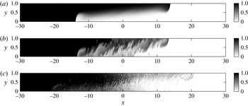
Figure 2 shows representative results for three configurations with identical parameter values
 $Re=10^{3}$
,
 $Pe_{T}=10^{3}$
and
 $R_{{\it\rho}0}=1.07$
, but different diffusivity ratios
 ${\it\tau}=1$
(single diffusive, top),
 $2/3$
(weakly double diffusive, middle) and
 $1/8$
(strongly double diffusive, bottom). All flow fields are shown at
 $t=30$
. The density difference between the lighter fluid in the left reservoir and the heavier fluid in the right one is seen to drive opposing gravity currents along the top and bottom walls. Superimposed on the primarily horizontal motion of these light (warm, salty) and dense (cold, fresh) gravity currents, double diffusion gives rise to strong fingering in the vertical direction. These fingers are driven by the release of potential energy stored in the unstable salinity stratification. While a fraction
 ${\it\xi}$
of this potential energy released by the salt is converted into potential energy of upwardly lifted colder fluid, linear stability investigations and nonlinear simulations of classical double-diffusive convection suggest that
 ${\it\xi}<1$
(Radko Reference Radko2013). As will be demonstrated in more detail below, double diffusion thus effectively reduces the density of the light top current, while increasing that of the heavy bottom current. As expected, lower diffusivity ratios (more disparate diffusivities) result in more intense double-diffusive fingering, and hence in the pronounced acceleration of the gravity currents for
 ${\it\tau}=1/8$
.
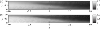
Salinity concentration for (a) a single-diffusive case with a diffusivity ratio
 ${\it\tau}=1$
, (b) a mildly double-diffusive case with
 ${\it\tau}=2/3$
and (c) a strongly double-diffusive case with
 ${\it\tau}=1/8$
. All flows have
 $R_{{\it\rho}0}=1.07$
and are shown for
 $t=30$
. At lower diffusivity ratios, the double-diffusive fingers are smaller and more numerous. Even for the mildly double-diffusive case with
 ${\it\tau}=2/3$
, the flow structure is quite different from that of a single-diffusive current, although the front velocity remains similar.

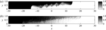
In figure 2 we note that the single-diffusive gravity current for
 $Re=10^{3}$
and
 ${\it\tau}=1$
is laminar. It is stable towards shear instabilities, and no Kelvin–Helmholtz instabilities form, as a suitably defined Richardson number would be above 0.25. For
 $Re=4\times 10^{3}$
, on the other hand, the single-diffusive current does form Kelvin–Helmholtz instabilities, as shown in figure 3(a), although their effect on the front velocity is small. For
 ${\it\tau}=1/8$
, the flow is dominated by double-diffusive fingering for both values of
 $Re$
, and Kelvin–Helmholtz instabilities can be identified at most in the vicinity of the current tip, where the fingering is less intense, as will be discussed in § 4.7.
Salinity concentration for (a) a single-diffusive case with a diffusivity ratio
 ${\it\tau}=1$
and (b) a strongly double-diffusive case with
 ${\it\tau}=1/8$
. Both flows have
 $R_{{\it\rho}0}=1.07$
and are shown for
 $t=30$
. Here
 $Re=4000$
, compared to figure 2, where
 $Re=1000$
.

This brief, qualitative description of the fundamental mechanisms at work suggests a strong coupling between the predominantly horizontal motion of the gravity currents and the primarily vertical double-diffusive fingering. To quantify the coupled dynamics as a function of the key governing dimensionless parameters
 $R_{{\it\rho}0}$
and
 ${\it\tau}$
represents the main goal of the present investigation. Towards this end, we perform a parametric study involving diffusivity ratio values
 ${\it\tau}=2/3,1/2,1/3,1/4,1/6,1/8$
and stability ratio values
 $R_{{\it\rho}0}=1.05,1.07,1.1,1.15,1.2,1.3,1.5$
. All simulations employ a fixed Reynolds number of
 $10^{3}$
, along with a temperature Péclet number of
 $10^{3}$
. For all parameter combinations with either
 $R_{{\it\rho}0}=1.07$
or
 ${\it\tau}=1/4$
, we perform ten simulations with slightly different random initial perturbations, so that we can obtain smoother data via ensemble averaging.
We initiate the simulations with an initial perturbation of white noise with an amplitude of 0.027 that is superimposed on an error function-shaped background initial condition
 $$\begin{eqnarray}T,S(x,y,t=0)=1-\text{erf}\left(\frac{x+0.027^{\ast }\text{rand}[-0.5,0.5](y)}{0.03}\right).\end{eqnarray}$$
While the flow fields of individual simulations for identical dimensionless parameter combinations exhibit similar qualitative behaviour, the ensemble averaging of ten simulations allows us to obtain smoother quantitative information.
4.1 Current length
We define the length
 $L(t)$
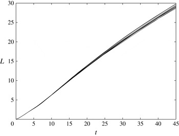
of the rightward propagating buoyant top current as the distance from the gate to the current tip, which is taken as the most advanced location with a dimensionless temperature of at least 0.05. Figure 4 shows
 $L(t)$
for all 10 simulations with
 $R_{{\it\rho}0}=1.07$
and
 ${\it\tau}=1/8$
. We observe that up until
 $t\approx 15-20$
the currents undergo a slight acceleration, whereas they tend to slow down moderately thereafter. At
 $t=45$
, the individual current lengths differ by up to 4 %.
Current length versus time for ten individual simulations with
 $R_{{\it\rho}0}=1.07$
and
 ${\it\tau}=1/8$
. Each simulation was initiated with a different random initial perturbation.

For a constant initial stability ratio
 $R_{{\it\rho}0}=1.07$
, figure 5(a) displays the ensemble-averaged current length
 $L(t)$
as function of
 ${\it\tau}$
. Keeping in mind that
 ${\it\tau}=1$
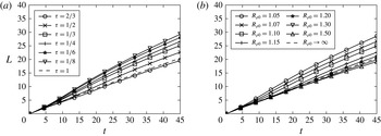
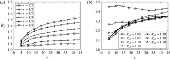
corresponds to classical, single-diffusive gravity currents, we find that strongly double-diffusive currents propagate up to 50 % faster than classical currents. We expect double diffusion to affect the current velocity via two opposing mechanisms: On one hand, double diffusion can modify the density contrast between a current and its ambient environment, which in turn will affect the current velocity. At the same time, double-diffusive fingering will increase the turbulent drag acting on the current, which should have a retarding effect. Interestingly, figure 5(a) indicates that the current velocity does not vary monotonically with
 ${\it\tau}$
. For
 ${\it\tau}$
-values slightly less than one, i.e. for weakly double-diffusive currents, we observe the current length to grow more slowly than for single-diffusive currents, whereas for strongly double-diffusive currents it grows more rapidly. This suggests that
 ${\it\tau}$
affects the balance between buoyancy and turbulent drag in a nonlinear fashion.
Current length versus time for
 $R_{{\it\rho}0}=1.07$
with varying
 ${\it\tau}$
(a), and for
 ${\it\tau}=1/4$
with varying
 $R_{{\it\rho}0}$
(b). Smaller values of
 ${\it\tau}$
or
 $R_{{\it\rho}0}$
, i.e. more strongly double-diffusive currents, result in larger front velocities. The single-diffusive case corresponds to
 ${\it\tau}=1$
in (a), and to
 $R_{{\it\rho}0}\rightarrow \infty$
in (b).

The above observations are consistent with earlier findings by Kimura & Smyth (Reference Kimura and Smyth2007), Smyth & Kimura (Reference Smyth and Kimura2007) and Smyth & Kimura (Reference Smyth and Kimura2011) on the interaction of double diffusion with shear. Those authors showed that for small values of
 ${\it\tau}$
the effective diffusivity of momentum is significantly smaller than that of the scalars.
A similar picture emerges regarding the influence of the initial stability ratio
 $R_{{\it\rho}0}$
when
 ${\it\tau}$
is held constant, cf. figure 5(b). Buoyant currents with
 $R_{{\it\rho}0}\rightarrow 1$
contain large quantities of both heat and salinity. Hence they are strongly double diffusive and quickly release substantial amounts of salt, so that their density decreases and they accelerate. Larger values of
 $R_{{\it\rho}0}$
, on the other hand, correspond to more weakly double-diffusive currents, for which the balance between buoyancy and turbulent drag becomes more complex, as will be discussed in more detail below. The limit
 $R_{{\it\rho}0}\rightarrow \infty$
corresponds to the classical, single-diffusive case.
4.2 Current structure: temperature, salinity, density and velocity
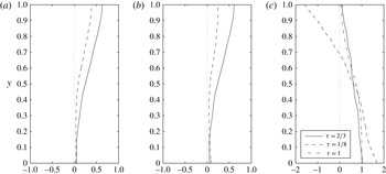
In order to provide quantitative evidence for the scenario outlined above, we now discuss the effective temperature and salinity profiles of the current. Towards this end, figure 6(a,b) displays vertical
 $T$
- and
 $S$
-profiles averaged in the streamwise direction from the gate position to the location half a channel height behind the current front. These figures demonstrate that the strongly double-diffusive top current (
 ${\it\tau}=1/8$
) loses both heat and salt more rapidly than its weakly double-diffusive counterpart (
 ${\it\tau}=2/3$
). In addition, it loses salt more quickly than heat, so that its effective density decreases. This is confirmed by the density profiles displayed in figure 6(c), which indicate that the dimensionless density of the strongly double-diffusive top current can reach values as low as
 $-$
1.5 near the upper boundary, far below the left reservoir value of
 ${\it\rho}=0$
. Similarly, the current density near the lower wall significantly exceeds the value
 ${\it\rho}=1$
in the right reservoir. The weakly double-diffusive current, on the other hand, loses heat and salinity at approximately the same rate, so that its effective density varies from
 ${\it\rho}=1$
near the bottom wall to
 ${\it\rho}=0$
near the top wall, similar to the single-diffusive gravity current. This increased buoyancy for the strongly double-diffusive current is consistent with the results shown in figure 2, where the strongly double-diffusive gravity current was seen to propagate much faster than its weakly double-diffusive counterpart. However, to fully understand the behaviour shown in figure 2, we will also have to consider the potentially higher drag acting on the strongly double-diffusive current, as a result of the fingering. We will return to this point further below.
Profiles averaged horizontally over the current length for (a) temperature
 $T$
, (b) salinity
 $S$
and (c) density
 ${\it\rho}$
, at time
 $t=45$
. All simulations have the same stability ratio
 $R_{{\it\rho}0}=1.07$
, whereas the diffusivity ratio
 ${\it\tau}$
takes the indicated values. Strongly double-diffusive currents lose their salinity more rapidly than their heat, in spite of the lower molecular diffusivity of salinity, so that the density difference driving the current increases.

The influence of
 $R_{{\it\rho}0}$
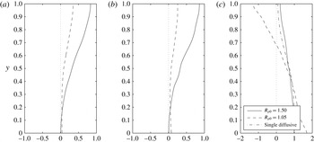
is consistent with the above arguments. Again, the strongly double-diffusive top current (
 $R_{{\it\rho}0}=1.05$
) loses both salt and heat much more rapidly than its weakly double-diffusive counterpart (
 $R_{{\it\rho}0}=1.50$
), cf. figure 7(a,b). It also loses salt faster than heat, so that its effective density decreases, as confirmed by the density profiles in figure 7(c).
Profiles averaged horizontally over the current length for (a) temperature
 $T$
, (b) salinity
 $S$
and (c) density
 ${\it\rho}$
, at time
 $t=45$
. All simulations have the same diffusivity ratio
 ${\it\tau}=1/4$
, whereas the stability ratio
 $R_{{\it\rho}0}$
takes the values indicated in the frames. Again, strongly double-diffusive currents lose their salinity more rapidly than their heat, so that the density difference driving the current increases.

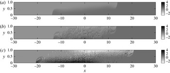
Density fields at
 $t=30$
for simulations with
 $R_{{\it\rho}0}=1.07$
and (a)
 ${\it\tau}=1$
(single diffusive), (b)
 ${\it\tau}=2/3$
(mildly double diffusive) and (c)
 ${\it\tau}=1/8$
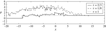
(strongly double diffusive). For the single-diffusive flow, the range of possible densities is bracketed by the reservoir values of 0 and 1. Double-diffusive flows, on the other hand, can give rise to local density values outside this range. Strongly double-diffusive flows display a local density maximum (minimum) near the bottom (top) centre of the domain.

For
 $R_{{\it\rho}0}=1.07$
, figure 8 compares the density fields of single-diffusive (
 ${\it\tau}=1$
), weakly double-diffusive (
 ${\it\tau}=2/3$
) and strongly double-diffusive (
 ${\it\tau}=1/8$
) currents. While the reservoir densities are identical for all flow fields, the current densities exhibit very different properties. The density of the single-diffusive current has to fall in between the reservoir densities, which is not true for the double-diffusive currents. The theoretical density limits for the light and heavy double-diffusive currents are given by
 $$\begin{eqnarray}\displaystyle & \displaystyle {\it\rho}(T=1,S=0)=1-\frac{R_{{\it\rho}0}}{R_{{\it\rho}0}-1}=-14.3, & \displaystyle\end{eqnarray}$$
 $$\begin{eqnarray}\displaystyle & \displaystyle {\it\rho}(T=0,S=1)=1+\frac{1}{R_{{\it\rho}0}-1}=15.3, & \displaystyle\end{eqnarray}$$
respectively. For the strongly double-diffusive case
 ${\it\tau}=1/8$
, we notice that the minimum and maximum fluid densities in the entire flow field appear near the upper and lower walls, in the neighbourhood of the gate location.
Density profiles along the bottom wall for the simulations with
 $R_{{\it\rho}0}=1.07$
at
 $t=30$
. For the single-diffusive current the density values have to fall in between the reservoir values of 0 and 1, respectively, while for the strongly double-diffusive current density values in excess of 4 appear near the gate location at
 $x=0$
.

The formation of this pool of high-density fluid along the bottom wall, which is confirmed by figure 9, strongly modifies the structure of the flow field. Since this fluid is significantly denser than the fluid in the right reservoir, it tends to spread horizontally along the bottom wall in both directions, and below the fluid of the right reservoir. Consequently, it deflects the left-moving current of right reservoir fluid upwards and away from the bottom wall. In this fashion, the flow field to the right of the original gate location acquires an effective three-layer structure, with a right-moving, light current along the top wall made up of warm and increasingly less salty fluid, a left-moving intermediate density current in the centre of the channel, and a pool of very dense, cold and salty fluid spreading horizontally along the bottom wall.
This emerging three-layer structure for strongly double-diffusive gravity currents (
 ${\it\tau}=1/8$
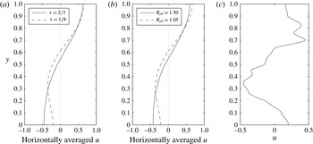
) is confirmed by the horizontally averaged
 $u$
-velocity profiles shown in figure 10(a). The weakly double-diffusive gravity current (
 ${\it\tau}=2/3$
), on the other hand, exhibits a clear two-layer structure, with a light top current moving to the right, and a dense bottom current moving to the left. Again, the influence of the parameter
 $R_{{\it\rho}0}$
is found to be consistent with these observations, as seen in figure 10(b). The weakly double-diffusive current for
 $R_{{\it\rho}0}=1.50$
displays a two-layer structure, while its strongly double-diffusive counterpart for
 $R_{{\it\rho}0}=1.05$
clearly has three distinct layers. The right-moving, dense current along the bottom wall can be clearly recognized in the local velocity profile of figure 10(c).
Horizontally averaged
 $u$
-profiles at
 $t=45$
: (a) for
 ${\it\tau}=2/3$
and
 $1/8$
, with
 $R_{{\it\rho}0}=1.07$
and (b) for
 $R_{{\it\rho}0}=1.50$
and 1.05, with
 ${\it\tau}=1/4$
. In each, the more strongly double-diffusive current develops a pronounced three-layer structure. (c) The
 $u$
-profile at
 $x=3$
for a simulation with
 $R_{{\it\rho}0}=1.07$
and
 ${\it\tau}=1/8$
. The right moving, very dense current next to the bottom wall is clearly visible, while the left-moving current containing fluid from the right reservoir has been deflected upwards, and away from the wall.

4.3 Current thickness
We now proceed to analyse the thickness of the buoyant top current. In order to be able to do so, we need to distinguish the current from the ambient. Towards this end, we define the interface location separating the top current from the ambient fluid below as the
 $y$
-location above which the horizontal volume flux in the positive
 $x$
-direction reaches a maximum. The condition of zero net horizontal volume flux implies that this
 $y$
-location also maximizes the horizontal volume flux in the negative
 $x$
-direction below. For a representative current with
 $R_{{\it\rho}0}=1.07$
and
 ${\it\tau}=1/4$
, figure 11 shows that the
 $y$
-position of the interface remains nearly constant over the length of the current. Consequently, we can evaluate an effective top current thickness by averaging the local thickness over the streamwise direction. In order to eliminate artefacts due to the current front, we take this streamwise average from the gate location to the position half a channel height behind the current front. We furthermore remark that, due to the initial transient flow evolution, a meaningful current thickness can be identified only after
 $t\approx 5$
.
Salinity concentration for a current with
 $R_{{\it\rho}0}=1.07$
and
 ${\it\tau}=1/4$
, at
 $t=35$
. The current interface, evaluated as described in the text, is drawn as a solid line. To obtain effective current properties such as temperature, salinity and thickness, we average from the gate location to half a channel height behind the current tip.

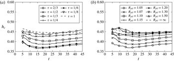
Figure 12(a) displays the current thickness as a function of time for
 $R_{{\it\rho}0}=1.07$
and various values of
 ${\it\tau}$
. During the acceleration phase until
 $t\approx 15{-}20$
, the current thickness decreases slightly, whereas subsequently it shows a mild increase as the current decelerates. While weakly double-diffusive currents have a thickness similar to that of single-diffusive currents, more strongly double-diffusive currents are seen to be increasingly thinner, as a result of the transition from a two-layer to a three-layer structure of the flow field, as described above. This trend is observed both for lower values of
 ${\it\tau}$
(figure 12
a) and for lower values of
 $R_{{\it\rho}0}$
(figure 12
b). We remark that the double-diffusive fingering also strongly affects the dissipation associated with the current.
Current thickness versus time for
 $R_{{\it\rho}0}=1.07$
with varying
 ${\it\tau}$
(a), and for
 ${\it\tau}=1/4$
with varying
 $R_{{\it\rho}0}$
(b). Smaller values of
 ${\it\tau}$
or
 $R_{{\it\rho}0}$
, i.e. stronger double diffusion, lead to thinner currents. The single-diffusive case corresponds to
 ${\it\tau}=1$
or
 $R_{{\it\rho}0}\rightarrow \infty$
.

It would be desirable to develop simplified, conceptual models in the spirit of Benjamin (Reference Benjamin1968) and/or Borden & Meiburg (Reference Borden and Meiburg2013) for predicting the velocity of double-diffusive currents as a function of their height. However, it is not obvious how those earlier models of steady, conservative currents could be extended to non-conservative, double-diffusive currents whose effective heat and salinity vary with time.
4.4 Temperature and salinity difference between the current and the ambient
We obtain the effective temperature and salinity of the buoyant top current by averaging over the area of the current, i.e. over the area above the interface from the gate location to the position half a channel height behind the tip. In order to quantify the temperature and salinity differences
 ${\rm\Delta}T$
and
 ${\rm\Delta}S$
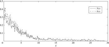
between the current and the ambient, we need to identify representative values for the temperature and salinity of the ambient. Towards this end, figure 13 shows the temperature and salinity, vertically averaged over the region below the interface, as functions of the streamwise
 $x$
-location for a representative flow. While the ambient has acquired significant amounts of heat and salinity near the gate location, its temperature and salinity values are close to zero over much of the length of the top current. For this reason, we assume the effective temperature and salinity values of the ambient to be zero, so that the
 ${\rm\Delta}T$
- and
 ${\rm\Delta}S$
-values between current and ambient are taken to be equal to the temperature and salinity of the current itself.
Vertically averaged temperature and salinity in the ambient as a function of
 $x$
, for a current with
 $R_{{\it\rho}0}=1.07$
and
 ${\it\tau}=1/8$
at
 $t=45$
. Over much of the length of the current,
 $T$
and
 $S$
in the ambient are close to zero.

Current temperature and salinity versus time for a weakly double-diffusive current with
 $R_{{\it\rho}0}=1.50$
and
 ${\it\tau}=1/4$
, and for a strongly double-diffusive current with
 $R_{{\it\rho}0}=1.07$
and
 ${\it\tau}=1/4$
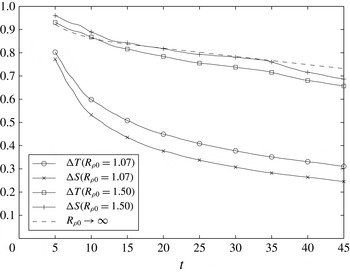
. The weakly double-diffusive current is seen to lose heat faster than salinity, which reflects the larger molecular diffusivity of heat, as compared to salt. The strongly double-diffusive current, on the other hand, loses salinity more rapidly than heat, as a result of the stronger turbulent diffusivity of salt, as compared to heat.

Figure 14 shows the resulting, ensemble-averaged results for
 ${\rm\Delta}T(t)$
and
 ${\rm\Delta}S(t)$
, for the weakly double-diffusive current with
 $R_{{\it\rho}0}=1.50$
and
 ${\it\tau}=1/4$
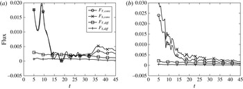
. These indicate that the temperature difference between the current and the ambient decays faster than the salinity difference, i.e. the weakly double-diffusive current loses heat more rapidly than salt. To identify the reasons for this behaviour, we evaluate the diffusive and convective fluxes of heat and salinity out of the current into the ambient according to
 $$\begin{eqnarray}F_{q,conv}(t)=-\frac{1}{L(t)-0.5}\int _{0}^{L(t)-0.5}vq\,\text{d}x,\end{eqnarray}$$
 $$\begin{eqnarray}F_{q,diff}(t)=\frac{1}{Pe_{q}(L(t)-0.5)}\int _{0}^{L(t)-0.5}\frac{\partial q}{\partial y}\,\text{d}x,\end{eqnarray}$$
where
 $q$
represents
 $T$
or
 $S$
, and the integrals are evaluated along an effective interface
 $y$
-location, which is taken as the actual
 $y$
-location of the interface averaged over the length of the current and from
 $t=5$
to
 $t=45$
. Figure 15(a) demonstrates that for the weakly double-diffusive current with
 $R_{{\it\rho}0}=1.50$
and
 ${\it\tau}=1/4$
the diffusive outflow of heat outweighs the diffusive outflow of salt for all times, as a result of the higher molecular diffusivity of heat as compared to salt. On the other hand, the convective fluxes of heat and salinity are nearly identical for early times, and mostly due to coherent vortical structures such as Kelvin–Helmholtz vortices, rather than double-diffusive fingering. At late times, fingering causes the convective outflow of salt to outweigh that of heat, and the combined diffusive and convective fluxes of heat and salt are nearly the same.
Diffusive and convective heat and salinity fluxes out of the top current, averaged from
 $x=0$
to
 $x=x_{tip}-0.5$
for (a) a weakly double-diffusive current with
 ${\it\tau}=1/4$
and
 $R_{{\it\rho}0}=1.50$
, and (b) a strongly double-diffusive current with
 ${\it\tau}=1/4$
and
 $R_{{\it\rho}0}=1.07$
. For both currents, the diffusive outflow of heat is larger than that of salinity. However, for the strongly double-diffusive current this effect is outweighed by the larger convective outflow of salt as compared to heat.

A very different picture emerges for the strongly double-diffusive current with
 $R_{{\it\rho}0}=1.07$
and
 ${\it\tau}=1/4$
, also shown in figure 14. In contrast to the weakly double-diffusive current the salinity difference now decays faster than the temperature difference, indicating that the current loses salt more rapidly than heat, in spite of the larger molecular diffusivity of heat. The reason for this becomes clear when we analyse the convective and diffusive fluxes of heat and salt out of the current, cf. figure 15(b). As expected, the diffusive outflow of heat from the current is larger than that of salt, due to the larger molecular diffusivity. However, this effect is outweighed by the larger convective outflow of salt, due to strong double-diffusive fingering. Hence, the effective turbulent diffusivity of salt is larger than that of heat, in spite of its molecular diffusivity being smaller.
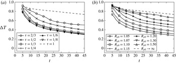
Figure 16 shows ensemble-averaged results for
 ${\rm\Delta}T(t)$
as function of
 ${\it\tau}$
and
 $R_{{\it\rho}0}$
, respectively. Corresponding plots of
 ${\rm\Delta}S(t)$
exhibit the same qualitative behaviour. Both parts of figure 16 indicate that
 ${\rm\Delta}T(t)$
decreases more quickly as the strength of the double-diffusive fingering increases. In the limit of
 ${\it\tau}\rightarrow 0$
,
 ${\rm\Delta}T(t)$
reaches an asymptotic limit. This reflects the fact that the effective diffusivity of heat depends on its molecular diffusivity as well as on the strength of the fingering, with the latter reaching an asymptotic limit as the molecular diffusivity of salt approaches zero, cf. also the analysis by Burns & Meiburg (Reference Burns and Meiburg2015). It is not immediately clear if a similar limit exists for
 $R_{{\it\rho}0}\rightarrow 1$
. We conclude that the presence of double-diffusive fingering strongly affects the temporal decay of temperature and salinity in the current, and thus the current’s driving force.
 ${\rm\Delta}T$
versus time for (a)
 $R_{{\it\rho}0}=1.07$
with varying
 ${\it\tau}$
, and (b) varying
 $R_{{\it\rho}0}$
with
 ${\it\tau}=1/4$
. The diffusivity of heat is the same in all simulations. Lower values of
 ${\it\tau}$
or
 $R_{{\it\rho}0}$
give rise to more intense double-diffusive fingering, which causes
 ${\rm\Delta}T$
to decay more rapidly. The single-diffusive case corresponds to
 ${\it\tau}=1$
or
 $R_{{\it\rho}0}\rightarrow \infty$
.

4.5 Effective buoyancy
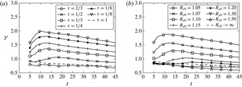
We can now employ (2.15) to calculate the effective density of the buoyant current, based on the results for
 ${\rm\Delta}T$
and
 ${\rm\Delta}S$
from § 4.4. Figure 17(a) indicates that, for constant
 $R_{{\it\rho}0}$
and varying
 ${\it\tau}$
, weakly double-diffusive currents are slightly less buoyant than single-diffusive currents. This is consistent with our earlier observation that they lose heat more rapidly than salt as a result of molecular diffusion, cf. figure 14. On the other hand strongly double-diffusive currents are significantly more buoyant than single-diffusive currents, since fingering causes them to lose salt much more rapidly than heat, as was also seen in figure 14. These findings are also consistent with our earlier observation that weakly double-diffusive currents propagate slightly more slowly than single-diffusive currents, whereas strongly double-diffusive currents advance much more rapidly. The results shown in figure 17(b) for varying
 $R_{{\it\rho}0}$
and constant
 ${\it\tau}$
confirm this scenario.
Density difference
 ${\it\gamma}$
versus time for (a)
 $R_{{\it\rho}0}=1.07$
and varying
 ${\it\tau}$
, and (b) varying
 $R_{{\it\rho}0}$
with
 ${\it\tau}=1/4$
. For strongly double-diffusive currents, the density difference can climb to twice the value of the reservoir fluids.

4.6 Energy budget
As shown in appendix A, the mechanical energy balance for a Boussinesq flow can be written as
 $$\begin{eqnarray}K+E_{p}+W_{c}+W_{d}=\text{const.}\end{eqnarray}$$
Here the kinetic energy
 $K$
is defined as
 $$\begin{eqnarray}K=\int \frac{u_{i}^{2}}{2}\,\text{d}A,\end{eqnarray}$$
while the gravitational potential energy
 $E_{p}$
has the form
 $$\begin{eqnarray}E_{p}=\int {\it\rho}x_{2}\,\text{d}A,\end{eqnarray}$$
and the energy lost to viscous dissipation is obtained as
 $$\begin{eqnarray}W_{d}=\frac{1}{Re}\int _{0}^{t}\int (\partial _{j}u_{i})(\partial _{j}u_{i})\,\text{d}A\,\text{d}t.\end{eqnarray}$$
The term
 $$\begin{eqnarray}W_{c}=-\int _{0}^{t}\int x_{2}\frac{\text{D}{\it\rho}}{\text{D}t}\,\text{d}A\,\text{d}t\end{eqnarray}$$
deserves some extra discussion, as it reflects the ways in which the diffusion of heat and salt affect the energy budget. Absent such diffusion, in an incompressible flow field each fluid particle maintains its density, so that
 $W_{c}=0$
. The way in which the diffusion of heat and salt influence the flow field via
 $W_{c}$
can be understood by exploring their role under simplified conditions. Imagine a stably stratified configuration of fluid at rest, consisting of a layer of warm fluid above a layer of colder fluid. In the absence of any initial perturbations, the fluid will stay at rest for all times, and the only transport that occurs is the downward diffusion of heat. This downward diffusion of heat implies that the density of fluid particles in the upper (lower) layer increases (decreases), giving a negative value of
 $W_{c}$
. In the energy equation (4.6), the negative
 $W_{c}$
is balanced by a positive change of
 $E_{p}$
, corresponding to an increase in potential energy. Winters et al. (Reference Winters, Lombard, Riley and D’Asaro1995) interpret
 $W_{c}$
in terms of the conversion of internal energy into potential energy via irreversible molecular processes, while Tailleux (Reference Tailleux2012) discusses
 $W_{c}$
in terms of the Boussinesq limit of the work performed due to fluid compression.
Now consider a stably stratified configuration consisting of a layer of warm, salty, lighter fluid above a layer of cold, fresh, denser fluid. In the absence of fluid motion, the only transport is the downward diffusion of heat and salt. As we saw above, the downward diffusion of heat gives a negative value of
 $W_{c}$
. On the other hand, the downward diffusion of salt reduces (increases) the density of the upper (lower) layer, thereby resulting in a positive value of
 $W_{c}$
. However, due to the larger molecular diffusivity of heat as compared to salt, the material density derivative due to the diffusion of heat outweighs that due to the diffusion of salinity, so that we expect the net effect of molecular diffusion to result in negative
 $W_{c}$
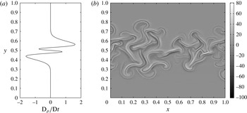
values. This is confirmed by figure 18(a), which shows a pronounced four-layer structure for
 $\text{D}{\it\rho}/\text{D}t$
at the interface. Figure 18(b) indicates that even in the presence of strong double-diffusive fingering, this four-layer structure of the material density derivative along the interface is maintained.
Material density derivative
 $\text{D}{\it\rho}/\text{D}t$
for hot, salty, light fluid above cold, fresh, dense fluid. (a) Molecular diffusion only, (b) with double-diffusive fingering. In each case, a pronounced four-layer pattern is observed along the interface.

In order to clarify the effect of vertical convective transport on
 $W_{c}$
, let us inspect the integral in (4.10) more closely. In a closed system such as the present one, the integral over
 $\text{D}{\it\rho}/\text{D}t$
vanishes. Now imagine a downward-moving finger carrying hot and salty fluid. As this fluid loses heat to its environment, it becomes increasingly denser, resulting in positive values of
 $\text{D}{\it\rho}/\text{D}t$
. At the same time, however, neighbouring fluid elements that absorb the heat released by the finger will see their density decrease. Conversely, upward-moving fingers become increasingly lighter as they absorb heat, leading to negative values of
 $\text{D}{\it\rho}/\text{D}t$
, while the surrounding fluid becomes denser. For hot and salty fluid at rest above cold and fresh fluid, figure 18(a) demonstrates that the four-layer structure results in
 $W_{c}$
being negative. Since figure 18(b) shows that this four-layer structure is maintained for double-diffusive fingering, we expect
 $W_{c}$
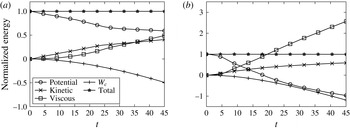
to remain negative even in the presence of flow. This is confirmed by figure 19, which shows the temporal evolution of all terms in (4.6) for a weakly and a strongly double-diffusive simulation, respectively, along with their sum. Here, all terms are scaled by the potential energy difference between the initial state and a hypothetical final state in which the upper half of the domain contains the lighter, hot and salty fluid, whereas the denser, cold and fresh fluid is located in the lower half. This limiting state would be reached for long times in the absence of any molecular diffusion of heat and salt. We refer to this energy difference as the ‘initially available potential energy’
 $\text{APE}_{0}$
. We observe that the sum of all energy components is preserved with very good accuracy for both flows.
For the weakly double-diffusive current in figure 19(a), we find that approximately 40 % of
 $\text{APE}_{0}$
is lost in the course of the simulation, and an approximately equal amount of kinetic energy is generated. An amount equivalent to approximately 60 % of
 $\text{APE}_{0}$
is dissipated by viscous forces, and roughly the same amount of mechanical energy is introduced into the flow field via the term
 $W_{c}$
.
Energy budget for a weakly double-diffusive current with
 $R_{{\it\rho}0}=1.07$
and
 ${\it\tau}=2/3$
(a), and a strongly double-diffusive current with
 $R_{{\it\rho}0}=1.07$
and
 ${\it\tau}=1/8$
(b). All energy components are scaled by the ‘initially available potential energy’
 $\text{APE}_{0}$
, as defined in the text. The potential energy released by the strongly double-diffusive flow far exceeds the initially available potential energy, reflecting the influence of double-diffusive fingering.

A qualitatively different picture emerges for the strongly double-diffusive current in figure 19(b). Here the amount of lost potential energy far exceeds
 $\text{APE}_{0}$
, which indicates that the buoyant, hot and salty current must have released some of the potential energy stored in the salinity field. In this context, it is useful to realize that the potential energy difference between the initial state and the theoretical limit of a layer of hot, fresh water above cold, salty water is
 $(R_{{\it\rho}0}+1)/(R_{{\it\rho}0}-1)$
times
 $\text{APE}_{0}$
. The amount of mechanical energy introduced into the flow by
 $W_{c}$
also exceeds
 $\text{APE}_{0}$
. By the end of the simulation, nearly three times
 $\text{APE}_{0}$
has been dissipated.
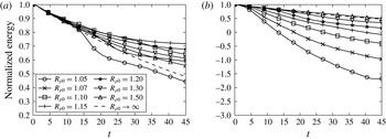
Figure 20(a) shows a comparison of the time evolution of gravitational potential energy for
 ${\it\tau}=2/3$
and various
 $R_{{\it\rho}0}$
. As explained earlier in § 4.4, for strong double-diffusive fingering the convective downward flux of salinity outweighs that of heat, resulting in a larger release of potential energy. Consequently, the current becomes lighter and propagates faster. As
 $R_{{\it\rho}0}$
increases, the dynamics of the current is governed by two competing effects. The intensity of the fingering decreases, which slows down the rate at which the potential energy of the salt is released. The fingering becomes very weak at
 $R_{{\it\rho}0}=1.20$
and non-existent at
 $R_{{\it\rho}0}=1.30$
, so that the potential energy budget becomes dominated by diffusion. The current now loses its heat faster than its salinity, so that it retains more of its potential energy than a single-diffusive current, and it propagates more slowly. As
 $R_{{\it\rho}0}$
increases further, the density contribution of the salinity decreases as compared to that of heat, and the current propagates faster again. Eventually, for large values of
 $R_{{\it\rho}0}$
its behaviour approaches that of a single-diffusive current. This observation is consistent with figure 5(b), which showed that the current is slowest for intermediate values of
 $R_{{\it\rho}0}$
.
Potential energy versus time for
 ${\it\tau}=2/3$
(a), and
 ${\it\tau}=1/8$
(b). In (a), when
 $R_{{\it\rho}0}$
is low enough to cause significant fingering, the fingering works to separate
 $T$
and
 $S$
, resulting in the release of more potential energy. When
 $R_{{\it\rho}0}$
is too high for fingering, further increases in
 $R_{{\it\rho}0}$
result in more potential energy being released because the salinity remaining in the current will contribute less to the density of the current and the current will spread faster. In (b), fingering is always strong, so decreasing
 $R_{{\it\rho}0}$
results in the release of more potential energy.

Figure 20(b) shows the corresponding graph for
 ${\it\tau}=1/8$
, where all of the currents exhibit strong fingering. In this case, changing
 $R_{{\it\rho}0}$
changes the release of gravitational potential energy in a monotonic way because the effect from fingering is always stronger than bulk diffusion. It is interesting to note that the presence of double-diffusive fingering enables more potential energy to be released than a single-diffusive current would have theoretically available. This is because some potential energy in the salinity field can be released in addition to the release of potential energy in the temperature field due to the motion of the current.
While double-diffusive currents generate more dissipation than their single-diffusive counterparts, i.e. they transfer more kinetic energy into internal energy, they also give rise to larger
 $W_{c}$
, so that they transfer more internal energy to potential energy. The magnitude of
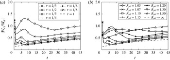
 $|W_{c}/W_{d}|$
provides insight into whether there is a net gain or loss of internal energy. Figure 21 displays this ratio for the usual parameter combinations. It is seen to be less than one for most currents, although for the weakly diffusive current with
 $R_{{\it\rho}0}=1.07$
and
 ${\it\tau}=2/3$
it exceeds this value for some period of time. Here it is important to keep in mind that not all of
 $W_{c}$
is necessarily converted into available potential energy. In the simple case of static cold fluid underneath warm fluid, heat diffuses downward, thereby increasing the potential energy. At the same time there is no dissipation, so that
 $|W_{c}/W_{d}|$
becomes infinite. The system remains in a state of minimum potential energy, and no potential energy is available for conversion into kinetic energy. Most interestingly, figure 21 indicates that the ratio
 $|W_{c}/W_{d}|$
is about the same for single-diffusive currents as for strongly double-diffusive currents, which suggests that strong fingering increases
 $W_{c}$
and
 $W_{d}$
by proportional amounts.
The ratio of
 $W_{c}/W_{d}$
versus time for (a)
 $R_{{\it\rho}0}=1.07$
with varying
 ${\it\tau}$
, and (b) varying
 $R_{{\it\rho}0}$
with
 ${\it\tau}=1/4$
. Strongly double-diffusive currents give rise to approximately the same ratio as single-diffusive currents, whereas weakly double-diffusive currents are characterized by a larger ratio.

4.7 Stability ratio
From the instantaneous temperature and salinity values of the current, we can calculate its effective stability ratio
 $R_{{\it\rho}}$
as a function of time. The ensemble-averaged results for
 $R_{{\it\rho}}$
shown in figure 22 are consistent with the earlier discussion in § 4.4. Strong double-diffusive fingering releases salt from the current more rapidly than heat, so that the stability ratio increases with time. However, this growth of
 $R_{{\it\rho}}$
tends to slow down over time since, as
 $R_{{\it\rho}}$
increases, the intensity of the double-diffusive fingering decreases. Conversely, in the absence of double-diffusive fingering, the current loses heat faster than salt, so that
 $R_{{\it\rho}}$
decreases with time. This is the case initially for
 ${\it\tau}=1/4$
and
 $R_{{\it\rho}0}=1.50$
. This decrease in
 $R_{{\it\rho}}$
tends to promote double-diffusive fingering, which in turn will slow down any further decrease of
 $R_{{\it\rho}}$
. As a result of these counterbalancing effects, we find that for
 ${\it\tau}=1/4$
all currents approach a stability ratio near 1.4 for long times, independent of their initial stability ratio. In figure 22(a), different values of
 ${\it\tau}$
lead to different long-term balances for the same
 $R_{{\it\rho}0}$
. Changing the value of
 ${\it\tau}$
modifies the strength of the effects of fingering and diffusion, which dictate the long-term balance, while changing
 $R_{{\it\rho}0}$
merely alters the initial condition. This effect applies not only in time, but also spatially, as fluid near the current front has had more time to adjust the local
 $R_{{\it\rho}}$
to reflect a balance of fingering and diffusive fluxes.
Stability ratio
 $R_{{\it\rho}}$
versus time for (a)
 $R_{{\it\rho}0}=1.07$
with varying
 ${\it\tau}$
, and (b) varying
 $R_{{\it\rho}0}$
with
 ${\it\tau}=1/4$
. Note that for
 ${\it\tau}=1/4$
, the stability ratio for all currents approaches 1.4 for long times, independent of the initial stability ratio
 $R_{{\it\rho}0}$
. On the other hand, for
 $R_{{\it\rho}0}=1.07$
, different values of
 ${\it\tau}$
result in different
 $R_{{\it\rho}}$
-values for long times.

4.8 Vertical velocity
In order to quantify the fingering intensity and the turbulent drag acting on the current, we evaluate the average magnitude
 $V$
of the vertical velocity along the interface from the gate location to
 $0.5$
dimensionless units behind the current tip
 $$\begin{eqnarray}V(t)=\frac{1}{N}\mathop{\sum }_{x_{i}=0}^{x_{i}\leqslant \text{tip}-0.5}|v(x_{i},\text{interface}(x_{i}),t)|,\end{eqnarray}$$
where
 $N$
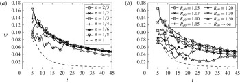
indicates the number of grid points included in the summation. Figure 23 shows representative, ensemble-averaged results for
 $V$
as a function of time.
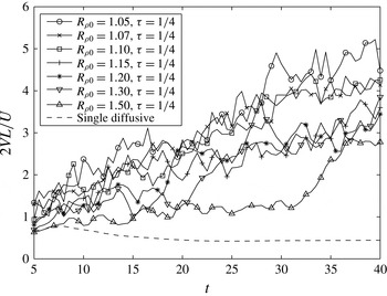
Average vertical velocity magnitude
 $V$
versus time for (a)
 $R_{{\it\rho}0}=1.07$
with varying
 ${\it\tau}$
, and (b) varying
 $R_{{\it\rho}0}$
with
 ${\it\tau}=1/4$
. Lower
 ${\it\tau}$
- or
 $R_{{\it\rho}0}$
-values (more intense double-diffusive fingering) initially produce larger vertical velocities, whereas for long times the velocity magnitude depends only weakly on
 $R_{{\it\rho}0}$
and
 ${\it\tau}$
.

For early times, parameter combinations giving rise to strong double-diffusive fingering result in larger values of
 $V$
. As either
 $R_{{\it\rho}0}$
or
 ${\it\tau}$
is held constant and the value of the other parameter is decreased to produce more intense fingering,
 $V(t)$
approaches an asymptotic relation. For constant
 $R_{{\it\rho}0}$
, this suggests that as
 ${\it\tau}$
is decreased,
 $R_{{\it\rho}}(t)$
increases in such a way that the overall fingering intensity remains about the same, which is consistent with figure 22(a). For constant
 ${\it\tau}$
, the existence of the asymptote reflects the fact that
 $R_{{\it\rho}}(t)$
approaches a constant value for all initial
 $R_{{\it\rho}0}$
, as had been seen in figure 22(b). For long times
 $V(t)$
decays for all currents, in line with the observations in § 4.7.
We remark that vertical velocities along the interface can be generated not only by double-diffusive fingering, but also as a result of the local thickening of the current behind the tip, as well as due to Kelvin–Helmholtz instabilities. For this reason even the single-diffusive current in figure 23(a) displays non-zero values of
 $V$
, although for all but the smallest times these are much lower than those due to double-diffusive fingering.
4.9 Late-stage dynamics
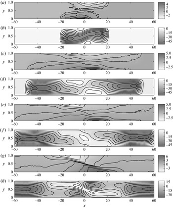
Streamlines in the laboratory reference frame and density contours at
 $t=25$
,
 $t=75$
,
 $t=100$
and
 $t=150$
. Density and velocity fields were smoothed using a moving average window with a width of 3 in
 $x$
. No smoothing was done in
 $y$
. A current with
 $R_{{\it\rho}0}=1.05$
and
 ${\it\tau}=1/8$
is shown. The size of the domain was
 $x\in [-120,120]$
, but only
 $x\in [-60,60]$
is shown. (a)
 ${\it\rho},t=25$
, (b)
 ${\it\psi},t=25$
, (c)
 ${\it\rho},t=75$
, (d)
 ${\it\psi},t=75$
, (e)
 ${\it\rho},t=100$
, (f)
 ${\it\psi},t=100$
, (g)
 ${\it\rho},t=150$
, (h)
 ${\it\psi},t=150$
.

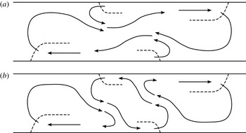
Sketches showing current fronts (dashed lines) and fluid motion (solid lines) before (a) and after (b) the transition to late-stage dynamics.

Heat (a) and salinity (b) near the centre of the domain at
 $t=100$
plotted with the true aspect ratio. In this region, denser hot and salty fluid exists under lighter cold and fresh fluid, leading to the diffusive instability.

Currents with sufficiently strong fingering to yield the three-layer structure described in § 4.2, exhibit long-term dynamics fundamentally different from the early stages. We will now discuss this for the representative case of
 $R_{{\it\rho}0}=1.05$
and
 ${\it\tau}=1/8$
shown in figure 24. We conducted a single large simulation with these parameters in an extended domain
 $x\in [-120,\,120]$
. The streamline pattern indicates that already at
 $t=25$
the pools of hot fresh fluid at the centre of the top wall, and cold salty fluid near the centre of the bottom wall have gained enough strength to deflect the original gravity current pattern, thereby resulting in the three-layer structure discussed above. However, the overall dynamics of the flow at this time is still governed by the right-moving top current and the left-moving bottom current.
By time
 $t=75$
, these localized pools along the top and bottom walls have become sufficiently strong to dominate the dynamics in the central region
 $-20\leqslant x\leqslant 20$
. Due to their strong density difference relative to the surrounding fluid, these pools tend to spread horizontally along their respective walls and give rise to new density fronts that propagate in the direction opposite to the original currents, so that a secondary, left-propagating top current emerges, along with a secondary, right-propagating current along the bottom wall. Initially, the fluid displaced by the secondary, left-moving top current forms a countercurrent immediately below that feeds into the original right-moving current along the same wall, as sketched in the streamline pattern in figure 25(a). A symmetric situation emerges along the bottom wall. By
 $t=100$
, however, the nature of the flow field has undergone a qualitative change due to a topological transition of the streamline pattern: the currents associated with the secondary fronts now form a closed recirculation zone in the central region that has cut off the primary currents from their original reservoirs, cf. figure 25(b). As a result, in the central region of the channel the local flow direction at
 $t=150$
is opposite to what it was at
 $t=25$
.
This closed recirculation region occupying the central section of the channel pushes hot and salty fluid underneath cold and fresh fluid, as shown in figure 26. A comparison of figure 26 to figure 24 confirms that in this region the hot, salty fluid is denser than the cold and fresh one, as it has lost more of its original heat than salinity. Hence this region becomes unstable to the ‘diffusive’ variant of the double-diffusive instability. The rapid upward diffusion of heat creates a layer of hot and fresh fluid just above the interface, along with cold and salty fluid just below it. These layers then drive ‘diffusive convection’ (Linden & Shirtcliffe Reference Linden and Shirtcliffe1978; Worster Reference Worster2004), which transports light fluid containing more heat than salinity upward, and dense fluid with more salinity than heat downward. As a result, the density gradient driving the secondary currents intensifies, cf. figure 24 at
 $t=150$
. Since the mixing above and below the interface is incomplete, some of the hot and salty fluid rises all the way to the top wall, where it forms a tertiary current flowing to the right, cf. figure 24 at
 $t=150$
. This current again displays the fingering instability, as seen in figure 26. In summary, in contrast to their single-diffusive counterparts, double-diffusive gravity currents display a much more complex long-term behaviour, which is characterized by the repeated generation of new density fronts.
5 Force balances
We begin by developing dimensional scaling arguments for the force balances, and subsequently convert these into dimensionless criteria. Following the approach of Maxworthy (Reference Maxworthy1983), we consider buoyancy, inertial, viscous and turbulent drag forces acting on the current. The turbulent drag due to vertical transport of horizontal momentum as a result of double-diffusive fingering can be estimated as
 $$\begin{eqnarray}F_{dd}\sim {\it\rho}_{0}UVL\sim {\it\rho}VL\frac{\text{d}L}{\text{d}t},\end{eqnarray}$$
where
 $U$
represents the horizontal velocity scale. Here we use
 $U\sim \text{d}L/\text{d}t$
, while Maxworthy (Reference Maxworthy1983) and Didden & Maxworthy (Reference Didden and Maxworthy1982) employed
 $U\sim L/t$
. These two approaches are equivalent as long as the power-law relationship between
 $L$
and
 $t$
remains constant for all times. By employing
 $U\sim \text{d}L/\text{d}t$
, we gain some flexibility in terms of allowing for temporal changes in the magnitude of the forces acting on the current, which may cause a transition from one power law to another. The inertial force per Maxworthy (Reference Maxworthy1983) and Didden & Maxworthy (Reference Didden and Maxworthy1982) scales as
 $$\begin{eqnarray}F_{i}\sim {\it\rho}_{0}U^{2}h_{c}\sim {\it\rho}_{0}\left(\frac{\text{d}L}{\text{d}t}\right)^{2}h_{c}.\end{eqnarray}$$
The viscous force is discussed at length by Didden & Maxworthy (Reference Didden and Maxworthy1982). For constant inflow, those authors develop spreading relations for top currents along slip boundaries, and for bottom currents along no-slip boundaries, governed by a balance of viscous and buoyancy forces. The currents are assumed to propagate into deep ambients, so that the drag on a bottom current is determined by the current thickness, while the drag on a top current is set by the growth of the shear layer into the ambient with time. In their experiments, however, the authors observe that even top currents seem to obey a no-slip boundary condition. They attribute this to impurities in the fluid, which cause the creation of a film on top of the current that effectively acts as a solid surface. Consequently, they assume that the viscous force scales with the current thickness even for a top current. While we have a clean, stress-free boundary in our numerical experiments, the ambient fluid layer is not deep, as the thickness of the current is roughly half the domain height. Consequently, the viscous force
 $F_{{\it\mu}}$
can be assumed to scale as
 $$\begin{eqnarray}F_{{\it\mu}}\sim {\it\mu}\frac{U}{h_{c}}L\sim {\it\mu}\frac{L}{h_{c}}\frac{\text{d}L}{\text{d}t}.\end{eqnarray}$$
The ratio of the double-diffusive to the viscous drag is thus given by
 $$\begin{eqnarray}\frac{F_{dd}}{F_{{\it\mu}}}\sim \tilde{V}\tilde{h}_{c}Re,\end{eqnarray}$$
where the tilde symbol indicates a dimensionless variable. Representative values for our numerically simulated currents are
 $\tilde{h}_{c}\approx 0.5$
and
 $\tilde{V}\approx 0.1$
, cf. figure 23. For typical simulation values of
 $Re=10^{3}$
, we hence estimate that the fingering drag
 $F_{dd}$
is roughly 50 times stronger than viscous drag
 $F_{{\it\mu}}$
.
The buoyancy force can be estimated by integrating the hydrostatic pressure difference between an idealized current shape and the ambient, as shown by Didden & Maxworthy (Reference Didden and Maxworthy1982) and Maxworthy (Reference Maxworthy1983)
 $$\begin{eqnarray}F_{b}\sim {\rm\Delta}{\it\rho}gh_{c}^{2}.\end{eqnarray}$$
For lock-release currents such as the ones considered here, the flow is always driven by the buoyancy force, which is balanced by one of the other forces. For currents driven by a supercritical forced inlet, Didden & Maxworthy (Reference Didden and Maxworthy1982) point out that the flow may be driven by inertia; however, that does not apply to the present situation.
5.1 Inertia–buoyancy balance
The spreading relationship for a current governed by an inertia–buoyancy balance can be derived by combining (5.2) and (5.5)
 $$\begin{eqnarray}{\it\rho}_{0}\left(\frac{\text{d}L}{\text{d}t}\right)^{2}h_{c}\sim {\rm\Delta}{\it\rho}gh_{c}^{2}.\end{eqnarray}$$
Consistent with our earlier numerical observations, we assume that the current thickness
 $h_{c}$
is constant with time, while
 ${\rm\Delta}{\it\rho}$
can vary with time. We thus obtain
 $$\begin{eqnarray}\frac{\text{d}L}{\text{d}t}\sim \sqrt{{\it\gamma}(t)g^{\prime }h_{c}},\end{eqnarray}$$
where
 ${\it\gamma}(t)$
represents the ratio of the instantaneous density difference driving the current to the initial density difference. By non-dimensionalizing and integrating in time we obtain
 $$\begin{eqnarray}\widetilde{L}\sim \int _{0}^{\widetilde{t}}\sqrt{{\it\gamma}(t^{\prime })}\,\text{d}t^{\prime }.\end{eqnarray}$$
The above differs from the analysis of Didden & Maxworthy (Reference Didden and Maxworthy1982) and Maxworthy (Reference Maxworthy1983) in two ways. Firstly, we allow for a time-dependent
 ${\it\gamma}(t)$
, and secondly, we assume
 $h_{c}$
is constant with time. In contrast, the earlier authors had assumed an additional relationship of the form
 $$\begin{eqnarray}Qt^{{\it\alpha}}=Lh_{c},\end{eqnarray}$$
where
 $Q$
indicates a constant.
5.2 Turbulent drag–buoyancy balance
We obtain the spreading relationship for a current governed by a fingering drag–buoyancy balance by combining (5.1) and (5.5)
 $$\begin{eqnarray}{\it\rho}VL\frac{\text{d}L}{\text{d}t}\sim {\rm\Delta}{\it\rho}gh_{c}^{2}.\end{eqnarray}$$
Non-dimensionalizing and integrating gives
 $$\begin{eqnarray}\widetilde{L}^{2}-\widetilde{L}_{s}^{2}\sim \int _{\widetilde{t}_{s}}^{\widetilde{t}}\frac{{\it\gamma}(\widetilde{t}^{\prime })}{\widetilde{V}}\,\text{d}\widetilde{t}^{\prime },\end{eqnarray}$$
where
 $\widetilde{t}_{s}$
indicates the transition time beyond which (5.11) first becomes valid and
 $\widetilde{L}_{s}$
represents the corresponding transition length. This balance corresponds to the one proposed by Maxworthy (Reference Maxworthy1983), except that here we assume
 $h_{c}$
to be constant, as discussed in the previous section, and we employ
 $U\sim \text{d}L/\text{d}t$
instead of
 $U\sim L/t$
.
5.3 Transition times
Hypothetically, if a certain force balance has been governing a current since
 $t=0$
and the current length
 $L$
obeys a power-law relationship with
 $t$
, the approximation
 $$\begin{eqnarray}\frac{\text{d}L}{\text{d}t}\sim \frac{L}{t}\end{eqnarray}$$
may be made and the proper scaling of
 $L$
with
 $t$
will be recovered. If it is assumed that
 ${\it\gamma}=1$
is constant, (5.8) simplifies to
 $$\begin{eqnarray}\widetilde{L}\sim \widetilde{t}.\end{eqnarray}$$
Assuming
 ${\it\gamma}=1$
and
 $\widetilde{V}$
constant and solving (5.11) for
 $L$
in a similar fashion, again using (5.12), gives
 $$\begin{eqnarray}\widetilde{L}\sim \sqrt{\frac{\widetilde{t}}{\widetilde{V}}}.\end{eqnarray}$$
Setting (5.14) equal to (5.13) and solving for
 $t$
gives an estimate of the time of the transition of the current from a inertia–buoyancy balance to a turbulent drag–buoyancy balance
 $$\begin{eqnarray}\widetilde{t}\sim \frac{1}{\widetilde{V}}.\end{eqnarray}$$
This is consistent with how Maxworthy (Reference Maxworthy1983) estimated transition times for his force balances. In light of our numerical findings, which show
 $\tilde{V}\approx 0.1$
(figure 23), this gives values of
 $O(10)$
for
 $\widetilde{t}$
.
5.4 Numerical evidence of force balances
5.4.1 Inertia–buoyancy balance
Figure 27 displays the ratio of the double-diffusive drag force (5.1) to the inertial force (5.2). We note that an inertia–buoyancy balance could at best be observed briefly for very early times, before the current becomes long enough for the fingering drag to dominate over inertia. However, as discussed above, the calculated current properties (
 $T$
,
 $S$
,
 ${\it\gamma}$
) are less reliable during these early stages, so that we do not observe a clear inertia–buoyancy stage for any of the double-diffusive currents. The single-diffusive current included in figure 27, while not having genuine double-diffusive fingering, nevertheless gives rise to vertical velocities along its interface, so that the evaluation of (5.1) results in a non-zero value. However, this value is much smaller than for any of the double-diffusive currents. An inertia–buoyancy balance can be observed for this single-diffusive current, as shown in figure 28(a), which plots the two sides of (5.8) against each other. The linear relationship through the origin for early times demonstrates the validity of (5.8).
Ratio of fingering drag to inertia force for various simulations showing that a pure inertia–buoyancy balance will not exist for currents with these parameters.

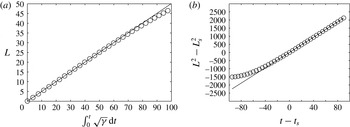
(a) Single-diffusive current: an inertia–buoyancy balance is observed, as indicated by the straight line, before viscous drag begins to become important. The circles represent the two sides of (5.8) plotted against each other. The solid line is a linear fit through the origin using data with
 $t\leqslant 50$
. (b) Double-diffusive current: test for a turbulent drag–buoyancy balance at later times. In the figure,
 $t_{s}=100$
and
 $L_{s}$
is the length of the current at
 $t=t_{s}$
. The fact that the data form a straight line through the origin shows that (5.11) holds in this time range.

5.4.2 Turbulent drag–buoyancy balance
Equation (5.15), with typical
 $V$
-values in the range [0.05, 0.10], provides an estimate of the transition time to a turbulent drag–buoyancy balance in the range
 $t\sim 10$
-20. In order to test for this turbulent drag–buoyancy balance, we carried out a long simulation until
 $t=190$
in a large control volume
 $x\in [-60,60]$
, for parameter values
 $R_{{\it\rho}0}=1.50$
and
 ${\it\tau}=1/8$
, which result in a moderate amount of fingering. Figure 28(b) plots the two sides of (5.11) against each other, with the additional assumption that
 ${\it\gamma}/V$
does not depend on time, which holds approximately for this simulation. In order to provide sufficient time for the transition to the turbulent drag–buoyancy balance to be completed, we choose
 $t_{s}=100$
, with
 $\tilde{L}_{s}$
denoting the current length at
 $t=t_{s}$
. The agreement of the simulation data with the straight line through the origin in figure 28(b) confirms the turbulent drag–buoyancy balance for long times.
There may be interesting implications of the above regarding the dynamics of double-diffusive intrusions. Ruddick, Phillips & Turner (Reference Ruddick, Phillips and Turner1999) observed a constant Froude number for intrusions driven by sugar and salt, suggesting a balance of inertia and buoyancy. However, at a value of 0.005 the Froude number was surprisingly small, which could not be explained by the authors. Although the diffusivities in the present simulations are much larger than those of sugar and salt, our results suggest that the intrusions of Ruddick et al. (Reference Ruddick, Phillips and Turner1999) could potentially have been driven by a buoyancy–fingering drag balance, with the appearance of a constant Froude number coming from an increase in the buoyancy of the intrusions over time. Because the length scales and velocities associated with the intrusions of Ruddick et al. (Reference Ruddick, Phillips and Turner1999) yield a much lower effective
 $Re$
than in the present simulations, we also cannot exclude the possibility that buoyancy and viscous forces were in balance, in accordance with (5.4). Either way, constant buoyancy would give a spreading relationship of
 $L\sim \sqrt{t}$
, whereas increasing buoyancy with time may result in a constant
 $Fr$
.
6 Comparison of two- and three-dimensional simulations
All of the simulations discussed up to this point were two-dimensional in nature. In order to explore the qualitative and quantitative agreement between two- and three-dimensional flows, we conducted a single three-dimensional run for
 $R_{{\it\rho}0}=1.07$
and
 ${\it\tau}=1/8$
. A visualization of the salinity isosurfaces at
 $t=14$
is shown in figure 29. Due to the high computational cost, this simulation employed a shorter domain in the
 $x$
-direction,
 $x\in [-10,\,10]$
, instead of
 $x\in [-30,\,30]$
as in the two-dimensional simulations. The grid size was
 $2049\times 257\times 257$
. The simulation was carried out until
 $t=15$
, at which time the current front approached the end wall. The properties of the three-dimensional current including the current length
 $L$
, the current thickness
 $h_{c}$
and the temperature and salinity differences between the current and the ambient,
 ${\rm\Delta}T$
and
 ${\rm\Delta}S$
, were calculated from the spanwise average of the simulation data.
Three-dimensional isosurfaces of the salinity concentration for
 $R_{{\it\rho}0}=1.07$
and
 ${\it\tau}=1/8$
, at
 $t=14$
. From dark to light, the contour values are 0.1, 0.3, 0.5, 0.7 and 0.9.

Comparison of the current length
 $L$
versus time
 $t$
for the two- and three-dimensional simulations with
 $R_{{\it\rho}0}=1.07$
and
 ${\it\tau}=1/8$
. The results indicate that the front velocity is not strongly affected by the third dimension.

Over the time interval of the simulations, the two- and three-dimensional currents propagate at nearly identical velocities, as shown in figure 30. This is consistent with earlier findings for single-diffusive gravity currents Härtel et al. (Reference Härtel, Meiburg and Necker2000) as well as turbidity currents Necker et al. (Reference Necker, Härtel, Kleiser and Meiburg2002). Nevertheless, there are noticeable differences in the dynamics of the currents even at these relatively early times, as will be seen in the following. Figure 31(a) indicates that soon after the start of the flow the thickness of the three-dimensional current drops by approximately 20 % compared to the equivalent two-dimensional current, which suggests that the fingering is considerably more intense in three than in two dimensions. This is confirmed by figure 31(b), which displays the temperature and salinity difference between current and ambient over time for both currents. The stronger fingering causes the three-dimensional current to exhibit a much more rapid decay of
 ${\rm\Delta}T$
and
 ${\rm\Delta}S$
. It is interesting to note that the front velocity remains nearly unchanged, in spite of the noticeable differences in current height,
 ${\rm\Delta}T$
and
 ${\rm\Delta}S$
.
Noticeable differences emerge between the two- and three-dimensional currents regarding their thickness
 $h_{c}$
(a), and their temperature and salinity difference with respect to the ambient,
 ${\rm\Delta}T$
and
 ${\rm\Delta}S$
(b). Parameter values are
 $R_{{\it\rho}0}=1.07$
and
 ${\it\tau}=1/8$
.

The three-layer structure discussed earlier in § 4.2 is seen to emerge again for three-dimensional currents, just as it had in two dimensions. Figure 32 compares streamwise-averaged
 $u(y)$
-profiles and local
 $u(y)$
-profiles at
 $x=1$
for the two- and three-dimensional simulations, where the three-dimensional flows have been averaged over the spanwise direction. The three-layer structure is somewhat less pronounced in three dimensions, but is clearly similar in nature.
 $u(y)$
-profiles at
 $t=15$
: (a) averaged over the streamwise extent of the current (and also over the spanwise direction for the three-dimensional flow), (b) local profile at
 $x=1$
(averaged over the spanwise direction for the three-dimensional flow). Parameter values are
 $R_{{\it\rho}0}=1.07$
and
 ${\it\tau}=1/8$
. The three-layer structure discussed earlier for two-dimensional flows emerges in three dimensions as well.

Slice of salinity concentration at
 $t=14$
normal to the vertical at
 $y=0.65$
, which is roughly the location of the current interface shown in figure 31(a).

Our finding that the three-dimensional current is similar to its two-dimensional counterpart but exhibits stronger fingering is consistent with results presented in Radko et al. (Reference Radko, Ball, Colosi and Flanagan2015) for flows with stochastic shear. This author’s work shows that fingering fluxes are larger in unsheared three-dimensional flows as compared to two dimensions, but that fluxes in a sheared three-dimensional environment are similar to two-dimensional fluxes in an unsheared environment. This is mainly due to the fact that shear causes three-dimensional fingers to align into salt sheets in the plane of the shear (Linden Reference Linden1974), since modes with non-zero wavenumber in this direction are damped. As a result, shear effectively reduces the dimensionality of the fingering from three to two dimensions, thereby reducing the flux by a factor of 2–3 (Radko et al. Reference Radko, Ball, Colosi and Flanagan2015). In two-dimensional gravity currents, the lack of the third dimension prevents any sheets from forming, and only modes with non-zero wavenumbers in the streamwise direction can grow. However, these modes will be damped in comparison to three dimensions, so that fluxes will be lower in the sheared two-dimensional environment.
The tendency of three-dimensional flows to form sheets is clearly visible in the horizontal slice of the salinity field displayed in figure 33. The slice shown is located at
 $y=0.65$
, which is roughly the height of the interface in figure 31(a). The sheet-like nature of the structures is more pronounced near the front of the current, where the shear at this
 $y$
-elevation may be more intense than near
 $x=0$
. In addition, this current section has been exposed to shear over a longer time interval, which may also contribute to its more sheet-like structure. A similar effect in horizontal cross sections of fingering in shear was also observed by Radko et al. (Reference Radko, Ball, Colosi and Flanagan2015).
7 Conclusions
The above simulations of lock-exchange flows in the Boussinesq regime demonstrate that strongly double-diffusive gravity currents in the fingering regime can exhibit quite different dynamics from their single-diffusive counterparts. Even at relatively modest Reynolds numbers, for which single-diffusive currents remain laminar, double-diffusive currents can give rise to pronounced small-scale fingering convection. By systematically varying the diffusivity ratio
 ${\it\tau}$
and the initial stability ratio
 $R_{{\it\rho}0}$
, we are able to quantify the influence of these parameters on the current evolution. Specifically, we notice that the propagation velocity of the current depends non-monotonically on these parameters. Strongly double-diffusive currents are seen to lose both heat and salinity more quickly than weakly double-diffusive ones. Furthermore, they lose salinity more quickly than heat, thereby increasing the initial density difference that drives them. This differential loss of heat and salinity results in the emergence of strong local density maxima and minima along the top and bottom walls in the gate region, which in turn promote the formation of secondary, counterflowing currents along the walls. These secondary currents result in a pronounced three-layer structure of the flow. In the neighbourhood of the gate region, the late stages of the flow are characterized by currents flowing in the opposite directions from the original ones, a phenomenon that bears some similarity to the buoyancy reversal observed for certain types of particulate gravity currents (Sparks et al.
Reference Sparks, Bonnecaze, Huppert, Lister, Hallworth, Mader and Phillips1993).
A detailed analysis of the energy budget shows that strongly double-diffusive currents can release several times their initially available potential energy. It furthermore elucidates the conversion of internal energy into mechanical energy via diffusion of the scalar fields. By quantifying the vertical fingering velocity, we are able to estimate the turbulent drag acting on the gravity current. Scaling arguments suggest that even at fairly low Reynolds numbers double-diffusive gravity currents are governed by a balance of buoyancy and turbulent drag, which is confirmed by the simulation results.
While the present simulations were motivated by thermohaline flows, the underlying model may also be applicable to flows in which one of the scalars contributing to the density is a particulate phase, as long as the influence of the settling velocity is small. For non-negligible settling velocities, on the other hand, novel phenomena can arise, as demonstrated in recent laboratory experiments (Parsons, Bush & Syvitski Reference Parsons, Bush and Syvitski2001), linear stability investigations (Burns & Meiburg Reference Burns and Meiburg2012; Yu, Hsu & Balachandar Reference Yu, Hsu and Balachandar2013) and nonlinear simulations (Yu, Hsu & Balachandar Reference Yu, Hsu and Balachandar2014; Burns & Meiburg Reference Burns and Meiburg2015). Similar considerations also apply to bioconvection in stratified environments (Karimi & Ardekani Reference Karimi and Ardekani2013).
As a final remark, we note that a related problem concerns the evolution of double-diffusive intrusions (Turner Reference Turner1978; Ruddick & Turner Reference Ruddick and Turner1979), for which the upper and lower interfaces may be subject to different instability modes. Work along these lines is currently under way.
Acknowledgements
The authors thank Professor P. Garaud for helpful discussions. E.M. gratefully acknowledges support through NSF grants CBET-1335148 and CBET-1438052. Some of the simulations were carried out at the Beach supercomputing facility at the University of Colorado at Boulder. Additional computational resources were provided by the Extreme Science and Engineering Discovery Environment (XSEDE), which is supported by National Science Foundation grant no. TG-CTS150053.
Appendix A. Derivation of energy budget
We begin by taking the dot product of (2.5) and velocity
 $\boldsymbol{u}$
to obtain
 $$\begin{eqnarray}(\partial _{0}u_{i})u_{i}+(u_{j}\partial _{j}u_{i})u_{i}=-(\partial _{i}P)u_{i}+\frac{1}{Re}(\partial _{j}\partial _{j}u_{i})u_{i}-({\it\rho}\hat{e}_{2})u_{i}.\end{eqnarray}$$
Making use of the continuity equation (2.4) gives a transport equation for
 $u_{i}^{2}/2$
 $$\begin{eqnarray}\partial _{0}\left(\frac{u_{i}^{2}}{2}\right)+u_{j}\partial _{j}\left(\frac{u_{i}^{2}}{2}\right)=-\partial _{i}(Pu_{i})+\frac{1}{Re}\left[\partial _{j}\partial _{j}\left(\frac{u_{i}^{2}}{2}\right)-(\partial _{j}u_{i})(\partial _{j}u_{i})\right]-{\it\rho}u_{2}.\end{eqnarray}$$
Integrating over the area of the domain and making use of continuity and the divergence theorem yields
 $$\begin{eqnarray}\partial _{0}\int \frac{u_{i}^{2}}{2}\,\text{d}A+\int \left(u_{j}\frac{u_{i}^{2}}{2}\right)\hat{n}_{j}\,\text{d}S=\frac{1}{Re}\left[\int \frac{\partial }{\partial \hat{n}}\left(\frac{u_{i}^{2}}{2}\right)\,\text{d}S-\int (\partial _{j}u_{i})(\partial _{j}u_{i})\,\text{d}A\right]-\int {\it\rho}u_{2}\,\text{d}A.\end{eqnarray}$$
Because of the no mass flux and free slip boundary conditions, the mechanical energy balance simplifies to
 $$\begin{eqnarray}\partial _{0}\int \frac{u_{i}^{2}}{2}\,\text{d}A+\int {\it\rho}u_{2}\,\text{d}A+\frac{1}{Re}\int (\partial _{j}u_{i})(\partial _{j}u_{i})\,\text{d}A=0.\end{eqnarray}$$
We define gravitational potential energy as
 $$\begin{eqnarray}E_{p}=\int {\it\rho}x_{2}\,\text{d}A.\end{eqnarray}$$
The time derivative of
 $E_{p}$
is
 $$\begin{eqnarray}\frac{\text{d}E_{p}}{\text{d}t}=\int x_{2}\frac{\partial {\it\rho}}{\partial t}\,\text{d}A=\int x_{2}\left(-u\boldsymbol{\cdot }\boldsymbol{{\rm\nabla}}{\it\rho}+\frac{\text{D}{\it\rho}}{\text{D}t}\right)\text{d}A=\int {\it\rho}u_{2}\,\text{d}A+\int x_{2}\frac{\text{D}{\it\rho}}{\text{D}t}\,\text{d}A.\end{eqnarray}$$
By rearranging this, we obtain
 $$\begin{eqnarray}\int {\it\rho}u_{2}\,\text{d}A=\frac{\text{d}E_{p}}{\text{d}t}-\int x_{2}\frac{\text{D}{\it\rho}}{\text{D}t}\,\text{d}A.\end{eqnarray}$$
By substituting (A 7) into (A 4), we arrive at
 $$\begin{eqnarray}\partial _{0}\int \frac{u_{i}^{2}}{2}\,\text{d}A+\frac{\text{d}E_{p}}{\text{d}t}-\int x_{2}\frac{\text{D}{\it\rho}}{\text{D}t}\,\text{d}A+\frac{1}{Re}\int (\partial _{j}u_{i})(\partial _{j}u_{i})\,\text{d}A=0.\end{eqnarray}$$
Integrating in time, one obtains
 $$\begin{eqnarray}\int \frac{u_{i}^{2}}{2}\,\text{d}A+E_{p}-\int _{0}^{t}\int x_{2}\frac{\text{D}{\it\rho}}{\text{D}t}\,\text{d}A\,\text{d}t+\frac{1}{Re}\int _{0}^{t}\int (\partial _{j}u_{i})(\partial _{j}u_{i})\,\text{d}A\,\text{d}t=\text{const.}\end{eqnarray}$$