



1. Introduction
In high-temperature industrial systems – such as gas turbine-cooling passages – the assumption of constant fluid properties becomes inadequate due to large temperature gradients and intense heat fluxes. In these environments, air or combustion gases flow through internal channels or over heated surfaces while undergoing significant thermal variations. These variations lead to substantial changes in key thermophysical properties, including density, viscosity and thermal conductivity. Such property gradients have a pronounced impact on both convective heat transfer and pressure losses, thereby requiring advanced modelling approaches capable of accurately capturing the coupled momentum–energy transport mechanisms.
It is well established that thermophysical property variations alter the turbulence dynamics, rendering classical scaling laws – derived under constant-property assumptions – inapplicable (Coles Reference Coles1961; Morkovin Reference Morkovin1962; Bradshaw Reference Bradshaw1977; Smits & Dussauge 2006). For compressible flows, various transformation techniques have been developed to establish similarity with incompressible, isothermal boundary layers. Notably, the transformation of Van Driest (Reference Van Driest1951) and the method proposed by Trettel & Larsson (Reference Trettel and Larsson2016) aim to collapse velocity profiles by accounting for variable density and viscosity effects. More recently, additional transformation frameworks have been proposed to improve scaling behaviour of supersonic wall-bounded flows, particularly for flows with non-adiabatic wall boundary conditions (Griffin, Fu & Moin Reference Griffin, Fu and Moin2021; Hasan et al. 2023).
To isolate the effects of property variation from compressibility, the present study focuses on incompressible flows with temperature-dependent thermophysical properties. This approach enables a more direct assessment of how thermophysical property variations – absent compressibility effects – influence the structure of turbulence and the transport of momentum and heat.
Patel, Boersma & Pecnik (Reference Patel, Boersma and Pecnik2017) addressed this question by conducting direct numerical simulations (DNS) of fully developed, internally heated channel flows with isothermal walls. They incorporated temperature-dependent constitutive relations for density, viscosity and thermal conductivity, and showed that the dominant effects of property variations on scalar transport can be effectively characterised using two non-dimensional parameters: the semi-local Reynolds number and the local Prandtl number. In particular, they demonstrated that near-wall gradients in the semi-local Reynolds number strongly influence turbulent heat flux generation through modifications to turbulence structure.
Complementing this perspective, Pecnik & Patel (Reference Pecnik and Patel2017) developed a modified turbulent kinetic energy (TKE) equation to account for strong near-wall gradients in density and viscosity. Their formulation, derived via a semi-local scaling of the Navier–Stokes equations, showed through budget analysis that the semi-local Reynolds number captures the leading-order effects of property variation in wall-bounded turbulent flows.
Zonta, Marchioli & Soldati (Reference Zonta, Marchioli and Soldati2012) conducted numerical simulations to investigate the behaviour of incompressible Newtonian fluids with anisotropic, temperature-dependent viscosity in forced convection turbulence. Their results showed that both mean and turbulent fields undergo significant variations. In particular, turbulence was found to be enhanced on the cold side of the channel, where viscosity is locally higher than the mean. Elevated viscosity values corresponded to an increase in TKE, whereas a reduction in TKE was observed near the hot wall. Analysis of the TKE budget revealed that these turbulence modifications are linked to changes in the rates of production and dissipation of TKE at the wall: specifically, production decreases at the hot wall and increases at the cold wall.
Lee et al. (Reference Lee, Jung, Sung and Zaki2013) performed DNS of turbulent boundary layers over isothermally heated walls to investigate the effects of viscosity stratification on turbulence statistics and skin friction. Using an empirical temperature-dependent viscosity model for water, two heated-wall cases were examined:
 $T_{w} = 70\,^\circ$
C and
 $T_{w} = 99\,^\circ$
C, where
 $T_w$
is the wall temperature, with a free-stream temperature of
 $30\,^\circ$
C. They found that wall heating reduces TKE in the buffer layer, accompanied by lower Reynolds shear stress and weaker turbulence production, while near-wall TKE increases due to enhanced energy transfer from viscosity stratification effects. Despite reduced viscosity near the wall, dissipation rises owing to intensified fine-scale motions. Wall heating reduced the skin-friction coefficient by up to 26 %, primarily due to changes in Reynolds shear stresses. Quadrant and octant analyses revealed significant reductions in ejections and sweeps, consistent with diminished outer vortical structures linked to ejection events.
Despite significant advances in understanding variable-property turbulent flows, a systematic characterisation of how thermophysical property variations alter the layered structure of wall-bounded turbulence remains incomplete. While transformation techniques are often used to recover velocity profile similarity with constant-property analogues, these methods may obscure the distinct physical mechanisms through which spatially varying viscosity and density modulate turbulent transport across different regions of the flow.
In contrast, the layer structure in constant-property wall-bounded flows has been extensively studied. From the classical four-layer description – viscous sublayer, buffer layer, logarithmic layer and wake layer (see e.g. Monin & Yaglom Reference Monin and Yaglom1965; Tennekes & Lumley Reference Tennekes and Lumley1972; Pope Reference Pope2001), to more recent mechanistic interpretations based on governing equations, much is known about the organisation of turbulent flows under uniform property conditions.
In particular, Wei et al. (Reference Wei, Fife, Klewicki and McMurtry2005) used a scaling-patch analysis of the mean momentum equation (MME) to identify four dynamically distinct layers, defined by the leading-order balances among viscous, turbulent and pressure forces. In layer I, the viscous force balances the pressure gradient; in layer II, the viscous force balances the gradient of the Reynolds shear stress; in the outer layer IV, the Reynolds shear stress gradient balances the pressure gradient. Between them lies the meso-layer III, where all three forces contribute significantly.
The scaling-patch framework provides a systematic approach to characterise wall-bounded turbulence by delineating regions in which different forces dominate the MME. While it does not prescribe a scaling a priori, when combined with physical insight, the framework facilitates the derivation of local characteristic scales and the interpretation of emergent flow behaviours (Fife et al. Reference Fife, Klewicki, McMurtry and Wei2005a ; Fife Reference Fife2006; Fife, Klewicki & Wei Reference Fife, Klewicki and Wei2009).
The present study adopts this perspective to examine incompressible turbulent channel flows with temperature-dependent thermophysical properties. Large wall-normal temperature gradients induce spatial variations in viscosity and density, which in turn modify the force balances that define the turbulent layers. Within the scaling-patch framework, the emergence of additional dimensionless parameters reflects these altered momentum balances and is therefore a natural consequence of variable-property effects. Although the framework is not intended to provide direct predictions of friction or heat transfer, it offers a systematic basis for understanding how variable properties alter the scaling and organisation of turbulent layers.
Applying this methodology places stringent demands on data quality, as the analysis requires accurate evaluation of second-order derivatives in the mean velocity. Such requirements are typically met only through direct numerical simulation. Accordingly, we analyse the comprehensive DNS dataset recently produced by Modesti & Pirozzoli (Reference Modesti and Pirozzoli2024), who investigated turbulent channel flows with temperature-dependent thermophysical properties under both wall-heating and wall-cooling conditions. These simulations were conducted at a bulk Mach number of 0.2, thereby isolating the effects of property variations from compressibility.
To facilitate interpretation of the DNS results, the key simulation parameters for each case are summarised in table 1. The datasets are labelled as L# and H#, where L denotes simulations at lower Reynolds numbers and H at higher Reynolds numbers. The accompanying number specifies the temperature ratio
 $ T_m/T_w$
. For example,
 $\mathrm{L04}$
corresponds to a low-Reynolds-number simulation with strong heating (
 $ T_m/T_w = 0.4$
). The simulations cover a wide range of friction Reynolds numbers, from
 $ Re_\tau = 155$
to
 $ Re_\tau = 3200$
, and bulk-to-wall temperature ratios ranging from
 $ T_m/T_w = 0.4$
(strong heating) to
 $ T_m/T_w = 3$
(strong cooling). Further details about the numerical set-up and boundary conditions can be found in Modesti & Pirozzoli (Reference Modesti and Pirozzoli2024).
Summary of DNS simulation cases analysed in this study. Here,
 $ \textit{Re}_\tau = \overline {\rho }_{w} u_\tau \delta _c/\overline {\mu }_{w}$
is the friction Reynolds number,
 $T_m/T_w$
is the bulk-to-wall temperature ratio and the case labels follow the convention in Modesti & Pirozzoli (Reference Modesti and Pirozzoli2024). The parameter
 $\beta _\mu$
is defined in (3.17).

Table 1. Long description
The table presents a summary of DNS simulation cases analyzed in the study. It includes key simulation parameters for each case, with datasets labeled as L# and H#, where L denotes simulations at lower Reynolds numbers and H at higher Reynolds numbers. The accompanying number specifies the temperature ratio. The table has 16 rows and 5 columns. Column headers are Case label, T subscript w (K), Re subscript tau, T subscript m / T subscript w, and beta subscript mu. Row 1: L04, 800, 155, 0.4, -0.0249. Row 2: L05-A, 293.15, 212, 0.5, -0.0237. Row 3: L05-B, 800, 205, 0.5, -0.0190. Row 4: L07, 800, 255, 0.7, -0.0102. Row 5: L08, 800, 356, 0.8, -0.0062. Row 6: L15, 800, 663, 1.5, 0.0126. Row 7: L2, 293.15, 789, 2.0, 0.0274. Row 8: L25, 293.15, 902, 2.5, 0.0369. Row 9: L3, 293.15, 1051, 3.0, 0.0456. Row 10: H04, 800, 260, 0.4, -0.0230. Row 11: H05-A, 293.15, 360, 0.5, -0.0217. Row 12: H05-B, 800, 404, 0.5, -0.0172. Row 13: H07, 800, 617, 0.7, -0.0090. Row 14: H08, 800, 674, 0.8, -0.0057. Row 15: H15, 293.15, 861, 1.5, 0.0151. Row 16: H2, 293.15, 1028, 2.0, 0.0271. Row 17: H25, 293.15, 1224, 2.5, 0.0368. Row 18: H3, 293.15, 1420, 3.0, 0.0450. Row 19: VH05, 800, 680, 0.5, -0.0160. Row 20: VH2, 293.15, 3201, 2.0, 0.0236.
To illustrate the contrasting effects of wall heating and cooling, figure 1 presents (a,b) a schematic of the thermal boundary conditions, (c,d) snapshots of the instantaneous velocity field and (e,f) the corresponding distributions of mean density and dynamic viscosity. Modesti & Pirozzoli (Reference Modesti and Pirozzoli2024) reported striking differences in turbulent structure arising from strong temperature-dependent viscosity variations. Specifically, they observed that ‘the wall-heating case (
 $\mathrm{H05}$
-
 $\mathrm{A}$
), despite having a relatively low friction Reynolds number (
 $ \textit{Re}_\tau = 360$
), exhibits finer turbulent structures than typically expected at this Reynolds number… whereas the wall-cooling case (
 $\mathrm{H3}$
), with a much higher friction Reynolds number (
 $ \textit{Re}_\tau = 1420$
), lacks small-scale eddies. The flow appears as a low-pass filtered version of the heated case, retaining only the large-scale structures’. They pointed out that these changed are caused by the strong viscosity variations within the near-wall and core flow regions.
The bottom panel of figure 1 highlights pronounced spatial variations in density and viscosity near the wall, which strongly influence local momentum and heat transfer. In the wall-heating case, the temperature peaks at the wall, leading to increased viscosity and reduced density in the near-wall region. In contrast, the wall-cooling case exhibits the lowest wall temperature and viscosity, accompanied by a corresponding increase in density.
The distribution of viscosity across the channel depth plays an important role in shaping the turbulence structure. For wall heating, viscosity remains relatively low in the core region, enabling the persistence of fine-scale turbulent motions and promoting enhanced activity in the outer layer. In contrast, wall-cooling results in a substantial viscosity increase toward the channel centre, which suppresses small-scale fluctuations and yields a velocity field dominated by large-scale structures, as seen in the middle panel.
Illustration of wall heating- and wall-cooling effects in a turbulent channel flow of air with variable thermophysical properties. (a,c,e) wall-heating condition (case
 $\mathrm{H05\text{-}A}$
, with
 $T_m/T_w = 0.5$
and
 $ \textit{Re}_\tau = 360$
). (b,d,f) wall-cooling condition (case
 $\mathrm{H}3$
, with
 $T_m/T_w = 3$
and
 $ \textit{Re}_\tau = 1420$
).

2. Governing equations
For a fully developed, incompressible turbulent channel flow with variable thermophysical properties, the governing equations for the mean streamwise momentum and mean temperature can be written as (Modesti & Pirozzoli 2024)
 \begin{align} 0 & = \underbrace {- \frac {{\mathrm{d}} \overline {p}}{{\mathrm{d}} x}}_{\textit{PF}} \,+\, \Bigg \{ \underbrace {\frac {{\mathrm{d}}}{{\mathrm{d}}y} \bigg ( \overline {\mu } \frac {{\mathrm{d}} \overline {u}}{{\mathrm{d}} y } \bigg )}_{\textit{VF}_{I}} + \underbrace {\frac {{\mathrm{d}}}{{\mathrm{d}}y} \overline { \bigg ( {\mu }' \frac {{\mathrm{d}} u'}{{\mathrm{d}} y }} \bigg )}_{\textit{VF}_{\textit{II}}} \Bigg \} \, \underbrace {-\, \frac {{\mathrm{d}} (\overline {\rho }\kern-1pt \widetilde {\ u'' v''})}{{\mathrm{d}} y}}_{\textit{TF}}, \\[-28pt] \nonumber \end{align}
 \begin{align} 0 & = \frac {\overline {\rho }}{{\rho }_b} \frac {Q}{\delta _c} \,+\, \left \{ \frac {{\mathrm{d}}}{{\mathrm{d}}y} \bigg ( \overline {k} \frac {{\mathrm{d}} \overline {T}}{{\mathrm{d}} y } \bigg ) + \frac {{\mathrm{d}}}{{\mathrm{d}}y} \overline { \bigg ( {k}' \frac {{\mathrm{d}} T'}{{\mathrm{d}} y }} \bigg ) \right \} \,-\, \frac {{\mathrm{d}} (\overline {\rho } \, c_p \widetilde {T'' v''})}{{\mathrm{d}} y}. \\[0pt] \nonumber \end{align}
In this work, an overline denotes Reynolds averaging, while a tilde denotes Favre averaging. A superscript single prime (
 $'$
) indicates a fluctuation from the Reynolds average, and a superscript double prime (
 $''$
) indicates a fluctuation from the Favre average. The streamwise and wall-normal directions are denoted by
 $x$
and
 $y$
, respectively, with corresponding velocity components
 $u$
and
 $v$
. The symbols
 $\rho$
,
 $\mu$
,
 $k$
and
 $c_p$
represent density, dynamic viscosity, thermal conductivity and specific heat capacity, respectively.
In the mean heat equation,
 $Q$
represents a uniform heat flux, computed at each time step to maintain a constant bulk temperature
 \begin{align} T_b = \frac {1}{ {\rho }_b \, {u}_b {\delta _c}} \int _0^{\delta _c} \rho \, u \, T \, \text{d}y , \end{align}
where
 $\delta _c$
is the channel half-height,
 ${\rho }_b$
is the bulk density and
 ${u}_b$
is the bulk velocity, defined as
 \begin{align} {u}_b = \frac {1}{{\rho }_b {\delta _c}} \int _0^{\delta _c} \rho \, u \, \text{d}y . \end{align}
The present configuration assumes statistically steady conditions with no mean streamwise temperature variation; while this differs from spatially developing heated channel flows, it enables isolation of the local effects of property gradients on the near-wall dynamics.
In the MME, three distinct forces contribute to the balance: the pressure force, the viscous force (VF) and the turbulent force, the latter arising from the gradient of the Reynolds shear stress. The viscous force itself comprises two components. The first, denoted as
 $\mathrm{VF}_{\textit{I}}$
, arises from the mean viscosity interacting with the gradient of the mean velocity. The second,
 $\mathrm{VF}_{\textit{II}}$
, is unique to variable-property flows and reflects the contribution from viscosity fluctuations interacting with the gradient of velocity fluctuations.
A similar structure appears in the mean temperature equation. The total diffusive flux contains a term based on the mean thermal conductivity and the mean temperature gradient, as well as an additional term arising from fluctuations in thermal conductivity and temperature gradient. These fluctuating-property terms are absent in constant-property flows and represent an important mechanism through which property variations directly influence momentum and heat transport. Their magnitude and spatial distribution are key indicators of how thermophysical gradients reshape the layered structure of turbulence.
Ratio of total viscous force to the gradient of Reynolds shear stress,
 $(\mathrm{VF}_{\textit{I}} + \mathrm{VF}_{\textit{II}})/\mathrm{TF}$
, for turbulent channel flow with variable thermophysical properties: (a) strong wall-heating case (
 $\mathrm{H05\text{-}A}$
), (b) strong wall-cooling case (
 $\mathrm{H3}$
). The wall-normal distance is normalised by the channel half-height
 $\delta _c$
. Constant-property reference data (LM) are included from the independent DNS of Lee & Moser (Reference Lee and Moser2015).

Integrating the mean momentum and mean heat transport equations in the wall-normal direction gives
 \begin{align} \frac {- \overline {\rho }\kern-1pt \widetilde {\ u'' v''}}{\tau _{w\textit{all}}} & = 1 \,-\, \frac {y}{\delta _c} \,-\, \frac {\overline {\mu } \frac {{\mathrm{d}} \overline {u}}{{\mathrm{d}} y }}{\tau _{w\textit{all}}} \,-\, \frac {\overline { \bigg ( {\mu }' \frac {{\mathrm{d}} u'}{{\mathrm{d}} y } \bigg ) }}{\tau _{w\textit{all}}} , \end{align}
 \begin{align} \frac {- \overline {\rho } \, c_p \, \widetilde {T'' v''}}{q_{w\textit{all}}} & = 1 \,-\, \frac {1}{\delta _c} \int _0^y \frac {\overline {\rho }}{{\rho }_b} {\mathrm{d}}y \,-\, \frac {\overline {k} \frac {{\mathrm{d}} \overline {T}}{{\mathrm{d}} y }}{q_{w\textit{all}}} \,-\, \frac {\overline { \bigg ( {k}' \frac {{\mathrm{d}} T'}{{\mathrm{d}} y } \bigg ) }}{q_{w\textit{all}}} . \end{align}
It is well known that the viscous shear stress,
 $\overline {\mu } {\mathrm{d}} \overline {u}/{\mathrm{d}} y$
, and the molecular heat flux,
 $\overline {k} {\mathrm{d}} \overline {T}/{\mathrm{d}} y$
, decrease rapidly away from the wall (Monin & Yaglom Reference Monin and Yaglom1965; Tennekes & Lumley 1972). Similarly, the contributions from fluctuations in viscosity or thermal conductivity also diminish quickly with distance from the wall. Consequently, equations (2.5) and (2.6) indicate that the wall shear stress and wall heat flux serve as natural characteristic scales for the Reynolds shear stress and turbulent heat transport, respectively. Furthermore, in the outer region, both quantities vary approximately linearly with the wall-normal coordinate, approaching zero at the channel centreline.
3. Layer structure developed from scaling-patch analysis of governing equations
The scaling-patch approach offers a multi-scale framework for analysing turbulent wall-bounded flows by dividing the flow domain into scaling patches – spatial regions where the dominant balances in the governing equations yield admissible and self-consistent scalings (Fife et al. Reference Fife, Klewicki, McMurtry and Wei2005a ; Wei et al. Reference Wei, Fife, Klewicki and McMurtry2005; Fife Reference Fife2006; Fife et al. Reference Fife, Klewicki and Wei2009; Wei 2020). This method recognises that different flow regions are governed by distinct physical mechanisms and dominant force balances. Within each patch, a dominant-balance analysis is performed to simplify the governing equations and derive the appropriate scaling behaviour. Adjacent patches can be connected through asymptotic matching in intermediate overlap regions, ensuring a globally consistent flow description. By systematically capturing the multi-scale, layered structure of wall-bounded turbulence, the scaling-patch framework goes beyond classical similarity theories and provides a robust foundation for incorporating additional physical effects, including variable thermophysical properties and compressibility.
As shown in (2.1), the MME involves three terms: the total viscous force, the gradient of the Reynolds shear stress and the imposed pressure gradient. To assess the relative importance of these terms, we examine the ratio between pairs of forces. For instance, figure 2 shows the ratio of the total viscous force to the Reynolds shear stress gradient for the wall-heating case H05-A and the wall-cooling case H3. For comparison, DNS data for constant-property turbulent channel flows from Lee & Moser (Reference Lee and Moser2015) at
 $ \textit{Re}_\tau = 395, 550$
and
 $1000$
are also included. Across all cases, the force ratios exhibit similar qualitative behaviour. In the near-wall region, there exists a sublayer where the ratio is approximately −1, indicating that the viscous force is nearly balanced by the Reynolds shear stress gradient – corresponding to layer II in the four-layer structure proposed by Wei et al. (Reference Wei, Fife, Klewicki and McMurtry2005). Near the centre of the meso-layer, where the Reynolds shear stress reaches its maximum and its gradient approaches zero, the ratio diverges. In the outer layer (layer IV), the ratio tends toward zero, indicating that the dominant balance is between the imposed pressure gradient and the Reynolds shear stress gradient.
A closer inspection of figure 2 reveals that variable thermophysical properties affect the thicknesses of different layers. For example, layers II and III in the wall-heating case H05-A (
 $ \textit{Re}_\tau = 360$
) closely resemble those of a constant-property case at a higher Reynolds number (
 $ \textit{Re}_\tau = 550$
), as shown in figure 2(a). Conversely, the corresponding layers in the wall-cooling case H3 (
 $ \textit{Re}_\tau = 1420$
) resemble those of a lower-Reynolds-number constant-property flow around
 $ \textit{Re}_\tau = 550$
. This observation is consistent with the instantaneous velocity fields shown in figure 1, where the wall-cooling case displays smoother, large-scale-dominated structures, characteristic of lower turbulence intensities.
Figure 2 shows that, based on the relative magnitudes of the force terms in the MME, the incompressible turbulent channel flow can be divided into an outer layer, a meso-layer, a gradient-balance layer and a sublayer adjacent to the wall. Because the effects of variable properties in the inner regions are more complex, we first present the analysis of the outer layer, followed by the meso-layer, and finally the inner sublayers.
3.1. Outer scaling of the variable-property turbulent channel flow
In his seminal work on turbulent shear flow, Townsend (Reference Townsend1976) highlighted a fundamental observation: ‘Perhaps the most significant fact about turbulent flows is that, while geometrically similar flows are expected to be dynamically and structurally similar if their Reynolds numbers are the same, their structures are also very nearly similar for all Reynolds numbers which are large enough to allow turbulent flow.’
To explain this apparent Reynolds-number insensitivity, Townsend proposed a scale-interaction argument: ‘It is supposed that turbulent eddies of different sizes affect one another only if their sizes are comparable. Then interaction between large, energy-containing eddies and the much smaller viscous eddies takes place through a considerable number of intermediary stages, and they are completely independent except that the viscous eddies dissipate the energy lost by the large eddies. It follows that the motion on the large scale is essentially inviscid and so independent of the Reynolds number.’ This insight laid the foundation for what is now known as outer-layer similarity in high-Reynolds-number wall-bounded turbulence.
According to this framework, the large turbulent motions in the outer region become increasingly decoupled from viscosity and near-wall effects as the Reynolds number increases. As a result, the outer-layer structure approaches a Reynolds-number-invariant state at sufficiently high Reynolds numbers.
Morkovin (Reference Morkovin1962) reached a similar conclusion in his studies of compressible boundary layers with variable thermophysical properties. Based on typical spectra of vorticity and density, Morkovin argued that ‘the dynamics of supersonic boundary layers are governed by large-scale eddies, as at low speeds. …Even in presence of dissipation, the larger-scale motion may resemble the incompressible motion.’ These observations suggest that, despite the effects of compressibility and property variations, the dominant large-scale turbulent motions can retain characteristics resembling those found in incompressible flows, pointing to a degree of universality in outer-layer dynamics. Outer-layer similarity has been further confirmed by particle image velocimetry and filtered Rayleigh scattering experiments by Williams et al. (Reference Williams, Sahoo, Baumgartner and Smits2018) in hypersonic turbulent boundary layers at a Mach number of 7.5. Similarly, DNS of compressible turbulent channel flow by Modesti & Pirozzoli (Reference Modesti and Pirozzoli2016) reveal that the integral length scale in the outer layer remains unaffected.
In canonical wall-bounded incompressible turbulent flows, a common outer scaling employs the friction velocity
 $u_\tau$
and friction temperature
 $\theta _\tau$
to normalise the mean velocity and temperature deficits. This traditional outer scaling is illustrated in figure 3. While such scaling performs reasonably well for constant-property flows (Schlichting & Gersten 2016), figure 3 demonstrates that it does not fully collapse in variable-property turbulent flows.
(a) Traditional outer scaling of the mean velocity deficit using the friction velocity
 $u_\tau$
. (b) Traditional outer scaling of the mean temperature deficit using the friction temperature
 $\theta _\tau$
.

Figure 3. Long description
Panel A: A line graph shows the traditional outer scaling of the mean velocity deficit using the friction velocity. The x-axis is labeled y/delta_c, and the y-axis is labeled (u_c - u)/u_tau. The graph includes multiple data series represented by different symbols and colors, indicating heating and cooling conditions. A legend specifies the symbols and colors used for different conditions. Panel B: A line graph shows the traditional outer scaling of the mean temperature deficit using the friction temperature. The x-axis is labeled y/delta_c, and the y-axis is labeled (T_c - T)/theta_tau. Similar to Panel A, this graph also includes multiple data series represented by different symbols and colors, indicating heating and cooling conditions. A legend specifies the symbols and colors used for different conditions.
To address this limitation, we introduce a new outer scaling consistent with Townsend’s outer similarity hypothesis. Assuming a hierarchy of self-similar structures exists in the outer layer, a representative wall-normal location
 $y_o$
within this region can be selected to define reference scales for the flow variables. Within this framework, it is natural to scale quantities such as the mean velocity and mean temperature using their respective deficits from centreline or free-stream values, as these deficits more accurately reflect the dynamics governing the outer region. Accordingly, the outer-scaled (deficit) variables are defined as
 \begin{align} y^- & = \frac {\delta _c - y}{\delta _c - y_o}, \quad (\overline {u})^{-} = \frac {\overline {u}_c - \overline {u} }{\overline {u}_c - \overline {u}_o }, \quad (\overline {T})^{-} = \frac {\overline {T}_c - \overline {T} }{\overline {T}_c - \overline {T}_o }, \nonumber \\\quad (\overline {\rho }\kern-1pt\widetilde {\ u'' v''})^- & = \frac {\overline {\rho }\kern-1pt\widetilde {\ u'' v''}}{(\overline {\rho }\kern-1pt\widetilde {\ u'' v''})_o}, \quad (\overline {\rho } C_p \widetilde {T'' v''})^- = \frac {\overline {\rho } C_p \widetilde {T'' v''}}{(\overline {\rho } C_p \widetilde {T'' v''})_o} ,\end{align}
where
 $y_o$
denotes a location in the outer layer, and
 $\overline {u}_o$
,
 $\overline {T}_o$
,
 $(\overline {\rho }\kern-1pt\widetilde {\ u'' v''})_o$
,
 $(\overline {\rho } C_p \widetilde {T'' v''})_o$
are the mean velocity, mean temperature, Reynolds shear stress and turbulent heat transport at that location. Using the outer-scaled variables, the MME and mean heat equation in the outer region can be written as
 \begin{align} 0 & \approx \frac { \tau _{w\textit{all}} }{\delta _c} \frac {\delta _c - y_o}{(-\overline {\rho }\kern-1pt\widetilde {\ u'' v''})_o} \,-\, \frac {{\mathrm{d}} (\overline {\rho }\kern-1pt\widetilde {\ u'' v''})^- }{{\mathrm{d}} y^-}, \\[-28pt] \nonumber \end{align}
 \begin{align} 0 & \approx \frac { q_{w\textit{all}} }{\delta _c} \frac {\delta _c - y_o}{(-\overline {\rho } C_p \widetilde {T'' v''})_o} \frac {\int _0^y \overline {\rho }{\mathrm{d}}y}{\rho _b} \,-\, \frac {{\mathrm{d}} (\overline {\rho } C_p \widetilde {T'' v''})^- }{{\mathrm{d}} y^-}. \\[-12pt] \nonumber \end{align}
It can be easily shown that
 $(-\overline {\rho }\kern-1pt\widetilde {\ u'' v''})_o$
can be approximated as
 $(1 - y_o/\delta _c)\,\tau _{w\textit{all}}$
in the outer region (see (2.5)). Consequently, the first term in (3.2) approaches unity, satisfying the admissible scaling criteria within the scaling-patch framework (Fife 2006). Similarly, the outer-scaled mean heat equation (3.3) also meets the admissible scaling requirements.
It is also useful to note the relationship
 $y/\delta _c = 1- (1-y_o/\delta _c) y^-$
, which indicates that for a given
 $y_o/\delta _c$
, the new outer-normalised wall distance
 $y^-$
maps uniquely to
 $y/\delta _c$
. For example, if we chose
 $y_o/\delta _c=0.4$
, then
 $y/\delta _c = 1- 0.6 y^-$
. For consistency and ease of comparison with previous studies, the new outer-normalised data are presented versus
 $y/\delta _c$
rather than
 $y^-$
.
Figure 4(a) presents the outer-scaled Reynolds shear stress profiles under various heating and cooling conditions, together with reference constant-property results. Consistent with the well-known behaviour of fully developed incompressible turbulent channel flows, the Reynolds shear stress in the outer region exhibits an approximately linear decrease with wall-normal distance, and the variable-property data collapse closely onto the canonical linear trend.
Figure 4(b) shows the corresponding outer-scaled turbulent heat flux profiles, which exhibit an approximately linear decrease in the outer region, with small but systematic departures from strict linearity. These deviations reflect fundamental differences in the governing transport equations. In the MME, the pressure gradient – the dominant outer-region driving term – is constant, yielding a strictly linear Reynolds shear stress distribution. In contrast, the driving term in the mean heat equation is only approximately constant, as the mean density
 $\overline {\rho }$
in (2.2) varies weakly across the outer region (see figure 1), leading to the observed departures from perfect linearity in the turbulent heat flux.
New outer scaling of (a) turbulent transport of momentum (Reynolds shear stress) and (b) turbulent transport of heat using a reference location
 $y_o/\delta _c = 0.4$
. Results are compared with constant-property turbulent channel flow data from independent DNS by Kawamura et al. (Reference Kawamura, Ohsaka, Abe and Yamamoto1998), Kawamura, Abe & Shingai (Reference Kawamura, Abe and Shingai2000) and Abe, Kawamura & Matsuo (Reference Abe, Kawamura and Matsuo2001) at
 $ \textit{Re}_\tau = 640$
.

The new outer-scaling framework can also be applied to the mean velocity and temperature deficits, as illustrated in figure 5, using a reference location of
 $ y_o/\delta _c = 0.4$
. This value is selected arbitrarily, as long as it remains sufficiently far from the wall to avoid contamination by near-wall effects – particularly if low Reynolds numbers data are included. Alternative choices, such as
 $ y_o/\delta _c = 0.2$
or
 $ 0.5$
, are equally valid. To illustrate this, figure 6 presents the outer-scaled profiles using
 $ y_o/\delta _c = 0.2$
, demonstrating comparable collapse.
New outer scaling of (a) mean velocity deficit and (b) mean temperature deficit using a reference location
 $y_o/\delta _c = 0.4$
. Results are compared with constant-property turbulent channel flow data from independent DNS by Kawamura et al. (Reference Kawamura, Ohsaka, Abe and Yamamoto1998, Reference Kawamura, Abe and Shingai2000) and Abe et al. (Reference Abe, Kawamura and Matsuo2001) at
 $ \textit{Re}_\tau = 640$
.

Figure 5. Long description
Two line graphs depict the new outer scaling of mean velocity deficit and mean temperature deficit using a reference location. Panel A: The line graph shows the normalized mean velocity deficit on the vertical axis against the normalized wall-normal coordinate on the horizontal axis. The data points are color-coded to represent different conditions, with red indicating heating and blue indicating cooling. Filled symbols represent one set of data, while open symbols represent another. The legend indicates various parameter values. A dashed line represents a constant property, and a dotted line represents a logarithmic relationship. Panel B: The line graph shows the normalized mean temperature deficit on the vertical axis against the normalized wall-normal coordinate on the horizontal axis. Similar color-coding and symbol conventions are used as in Panel A. The graphs compare results with constant-property turbulent channel flow data from independent DNS by Kawamura et al. and Abe et al. at specific conditions.
New outer scaling of (a) mean velocity deficit and (b) mean temperature deficit using a reference location
 $y_o/\delta _c = 0.2$
.

Figures 5 and 6 demonstrate that the outer-scaling defined in (3.1) yields a consistent collapse of the mean velocity and temperature deficit profiles across a wide range of Reynolds numbers and thermal boundary conditions, including wall-heating, wall-cooling and constant-property cases. These results support the concept of outer-layer similarity – originally developed for incompressible flows and later extended to compressible flows with property variations.
Moreover, the results indicate that the decrease of the mean velocity and temperature deficits in the outer layer can be approximated by a logarithmic function
 \begin{align} \frac {\overline {u}_c - \overline {u}}{\overline {u}_c - \overline {u}_o} \approx A \mathrm{ln}(y/\delta _c) + B, \end{align}
where the
 $A$
and
 $B$
values depend on the choice of
 $y_o/\delta _c$
. For example, figure 5(a) shows
 $ A = -1.2$
and
 $ B = -0.1$
for
 $ y_o/\delta _c = 0.4$
, while figure 6(a) shows that
 $ A = -0.7$
and
 $ B = -0.1$
for
 $ y_o/\delta _c = 0.2$
. Interestingly, the temperature deficit exhibits nearly identical coefficients, suggesting a common outer-layer behaviour for both velocity and thermal fields.
3.2. Variable-property effects within the meso-layer
The existence of a meso-layer in wall-bounded turbulent flows was first proposed by Long & Chen (Reference Long and Chen1981) and Afzal (Reference Afzal1982). In the four-layer framework introduced by Wei et al. (Reference Wei, Fife, Klewicki and McMurtry2005), the meso-layer (layer III) is centred about the location of the peak Reynolds shear stress, denoted by
 $y_{_\textit{RSmax}}$
. Figure 7 illustrates how both the location and magnitude of this peak vary with Reynolds number. As the Reynolds number increases under either wall-heating or wall-cooling conditions,
 $ y_{_\textit{RSmax}}/\delta _c$
decreases, indicating that the peak shifts closer to the wall. At the same time, the peak Reynolds shear stress increases, asymptotically approaching the wall shear stress.
Figure 7 also highlights the pronounced sensitivity of both
 $y_{_\textit{RSmax}}$
and the maximum Reynolds shear stress magnitude to thermal boundary conditions. Wall heating and cooling significantly alter the distribution of turbulence stresses, thereby modifying the structure and extent of the meso-layer.
Effect of Reynolds number and thermal boundary conditions on the peak location and magnitudes of Reynolds shear stress.

At
 $y_{_\textit{RSmax}}$
, the gradient of the Reynolds shear stress vanishes, i.e.
 $\mathrm{d}(\overline {\rho }\,\widetilde{\ u''v''})/\mathrm{d}y = 0$
. As a result, the MME (2.1) evaluated at
 $y_{_\textit{RSmax}}$
reduces to
 \begin{align} 0 & = \frac {\tau _{w}}{\delta _c} \,+\, \Bigg ( \frac {{\mathrm{d}} \overline {\mu }}{{\mathrm{d}} y} \frac {{\mathrm{d}} \overline {u}}{{\mathrm{d}} y} \Bigg )_{y_{_\textit{RSmax}}} \,+\, \Bigg ( \overline {\mu } \frac {{\mathrm{d}}^2 \overline {u}}{{\mathrm{d}} y^2} \Bigg )_{y_{_\textit{RSmax}}} \,+\, \Bigg ( \frac {{\mathrm{d}}}{{\mathrm{d}}y} \overline { {\mu }' \frac {{\mathrm{d}} u'}{{\mathrm{d}} y }} \Bigg )_{y_{_\textit{RSmax}}}. \end{align}
Figure 8 presents the individual terms of the MME evaluated at
 $y_{_\textit{RSmax}}$
. The results indicate that the contributions from viscous forces associated with viscosity variations or fluctuations are negligible at this location. Accordingly, the MME at
 $y_{_\textit{RSmax}}$
can be simplified as
 \begin{align} \Bigg ( \overline {\mu } \frac {{\mathrm{d}}^2 \overline {u}}{{\mathrm{d}} y^2} \Bigg )_{y_{_\textit{RSmax}}} & \approx - \frac {\tau _{w}}{\delta _c}. \end{align}
Terms in the MME (3.5) at the maximum Reynolds shear stress location
 $y_{_\textit{RSmax}}$
. The terms are normalised by
 $u_\tau$
and
 $\nu _{w}/u_\tau$
.

Since the seminal work of Prandtl and von Kámán in the early 1930s, it has been well established that wall-bounded turbulent flows with constant fluid properties – such as channel, pipe and flat-plate boundary layers – feature a region in which the mean velocity and temperature profiles display approximately logarithmic behaviour. These profiles are commonly expressed as
 \begin{align} \frac {\overline {u}}{u_\tau } \approx \frac {1}{\kappa } \ln \left (\frac {y u_\tau }{\nu _{w}}\right ) + C, \end{align}
where
 $\kappa$
is the von Kármán constant, and
 $C$
is an additive constant. The existence of this logarithmic layer has been supported by numerous experimental and numerical studies, confirming its robustness. Although no universal value exists for
 $\kappa$
across different geometries, it remains approximately constant for a given configuration and is largely insensitive to the Reynolds number (Nagib & Chauhan 2008).
In turbulent channel flows with variable fluid properties, a logarithmic layer also emerges at sufficiently high Reynolds numbers (Modesti & Pirozzoli 2024). However, the additive constant
 $C$
is modified due to variations in fluid properties such as viscosity and thermal conductivity.
At sufficiently high Reynolds number, the location of maximum Reynolds shear stress,
 $y_{_\textit{RSmax}}$
, is expected to reside within the logarithmic layer. Consequently, the MME evaluated at
 $y_{_\textit{RSmax}}$
(3.6) may be approximated using the logarithmic form of the mean velocity
 \begin{align} \overline {\mu }_{_\textit{RSmax}} \frac {u_\tau }{\kappa \, y^2_{_\textit{RSmax}}} & \approx \frac {\tau _{w}}{\delta _c}. \end{align}
This approximation leads to an estimate for the location of the maximum Reynolds shear stress
 \begin{align} \frac {y_{_\textit{RSmax}}}{\delta _c} \approx \frac {1}{\sqrt {\kappa }} \frac {1}{\sqrt {\rho _{w} u_\tau \delta _c/\overline {\mu }_{_\textit{RSmax}}}} = \frac {1}{\sqrt {\kappa }} \frac {1}{\sqrt {Re_\tau }\,\sqrt { \overline {\mu }_{w}/\overline {\mu }_{_\textit{RSmax}}}} . \end{align}
Applying the log-law approximation for the mean velocity gradient in the integrated MME (2.5), the maximum Reynolds shear stress can be estimated as
 \begin{align} 1 - \frac {(-\overline {\rho }\kern-1pt\widetilde {\ u'' v''})_{\textit{max}}}{\tau _{w}} & \approx \frac {y_{_\textit{RSmax}}}{\delta _c} + \frac {\bigg ( \overline {\mu } \frac {{\mathrm{d}} \overline {u}}{{\mathrm{d}} y} \bigg )_{_\textit{RSmax}}}{\tau _{w\textit{all}}} \nonumber \\ & \approx \frac {y_{_\textit{RSmax}}}{\delta _c} + \frac { \overline {\mu }_{_\textit{RSmax}} \frac {u_\tau }{\kappa } \frac {1}{ y_{_\textit{RSmax}} } }{ \tau _{w\textit{all}}} \nonumber \\ & \approx \frac {2}{\sqrt {\kappa }} \frac {1}{\sqrt {\rho _{w} u_\tau \delta _c/\overline {\mu }_{_\textit{RSmax}}}} = \frac {2}{\sqrt {\kappa }} \frac {1}{\sqrt {Re_\tau }\,\sqrt { \overline {\mu }_{w}/\overline {\mu }_{_\textit{RSmax}}}}, \end{align}
where the factor of
 $2$
arises because, at the location of the maximum Reynolds shear stress, the two terms on the right side of the first line in (3.10) are of equal magnitude.
For constant-property turbulent channel flows, these equations recover the previously reported scalings:
 $y_{_\textit{RSmax}}/\delta _c \sim 1/\sqrt { Re_\tau }$
or
 $y^+_{_\textit{RSmax}} \sim \sqrt {Re_\tau }$
(Long & Chen Reference Long and Chen1981; Afzal Reference Afzal1982; Sreenivasan & Sahay Reference Sreenivasan and Sahay1997; Wei et al. 2005) and
 $1-(-\overline {u'v'})^+_{\textit{max}} \sim 1/\sqrt {Re_\tau }$
(Fife et al. Reference Fife, Wei, Klewicki and McMurtry2005b
).
Figure 9 illustrates the effects of variable properties and Reynolds number on the location
 $y_{_\textit{RSmax}}$
. For comparison, data from constant-property flows are also included. As shown in figure 9(a), the normalised peak location
 $y_{_\textit{RSmax}}/\delta _c$
exhibits a similar trend for both variable- and constant-property flows. To better highlight the Reynolds-number dependence, figure 9(b) presents
 $y_{_\textit{RSmax}}/\delta _c$
multiplied by
 $\sqrt {Re_\tau \overline {\mu }_{w}/\overline {\mu }_{_\textit{RSmax}}}$
. This quantity tends toward an asymptotic constant at high Reynolds numbers, consistent with the prediction from (3.9). The deviations observed for
 $ \textit{Re}_\tau \lesssim 2000$
are attributed to the breakdown of the log-law approximation at the
 $y_{_\textit{RSmax}}$
location under low-Reynolds-number conditions. For example, at
 $ Re_\tau = 180$
, the peak Reynolds shear stress occurs at
 $ y^+_{_\textit{RSmax}} \approx 31$
, which lies outside the region where the logarithmic velocity profile is valid.
In variable-property flows, wall-heating cases closely follow the trend of constant-property flows. In contrast, wall-cooling cases exhibit noticeable deviations – particularly at lower Reynolds numbers. This behaviour also stems from the limitations of the log-law approximation in the derivation: under wall-cooling conditions, the onset of the logarithmic layer shifts outward.
Location of the maximum Reynolds shear stress in turbulent channel flow with variable property: (a) peak location normalised by the channel half-height,
 $y_{_\textit{RSmax}}/\delta _c$
; (b) same quantity multiplied by
 $\sqrt {Re_\tau \overline {\mu }_{w}/\overline {\mu }_{_\textit{RSmax}}}$
. Filled red and blue symbols denote the low-Reynolds-number DNS of Modesti & Pirozzoli (Reference Modesti and Pirozzoli2024), while open symbols correspond to higher Reynolds numbers; the largest open symbols indicate their highest-Reynolds-number case. Constant-property reference data are taken from the DNS of Lee & Moser (Reference Lee and Moser2015) (LM) and Kawamura’s group (Kawamura et al. Reference Kawamura, Ohsaka, Abe and Yamamoto1998, Reference Kawamura, Abe and Shingai2000; Abe et al. 2001) (K)).

Figure 9. Long description
Two scatter plots depict the location of the maximum Reynolds shear stress in turbulent channel flow with variable property. Panel A: A scatter plot shows the peak location normalized by the channel half-height. The x-axis represents the Reynolds number, and the y-axis represents the normalized peak location. Red symbols denote heating, and blue symbols denote cooling. Filled symbols represent low-Reynolds-number DNS, while open symbols correspond to higher Reynolds numbers. The largest open symbols indicate the highest-Reynolds-number case. Panel B: A scatter plot shows the same quantity multiplied by the square root of the density ratio. The x-axis represents the Reynolds number, and the y-axis represents the normalized and scaled peak location. The same color and symbol scheme is used as in Panel A. The dashed lines represent constant-property reference data from DNS.
Figure 10 illustrates the influence of variable fluid properties and Reynolds number on the peak Reynolds shear stress. To assess the validity of (3.10), figure 10(b) plots the product
 $ \sqrt {Re_\tau \overline {\mu }_{w}/\overline {\mu }_{_\textit{RSmax}}} (1 - (-\overline {\rho }\kern-1pt\widetilde {\ u'' v''})_{\textit{max}} / \tau _{w} )$
. For constant-property flows, this value asymptotes to approximately 3 at
 $ Re_\tau \gtrsim 1000$
. The variable-property cases display a qualitatively similar trend; however, noticeable deviations occur in wall-cooling scenarios at lower Reynolds numbers.
Peak values of the Reynolds shear stress in turbulent channel flows with variable thermophysical properties. (a) Deficit of the peak Reynolds shear stress from 1, normalised by the wall shear stress
 $\tau _{w}$
; (b) same quantity multiplied by
 $\sqrt {Re_\tau }$
. Filled red and blue symbols denote the low-Reynolds-number DNS of Modesti & Pirozzoli (Reference Modesti and Pirozzoli2024), while open symbols correspond to higher Reynolds numbers; the largest open symbols indicate their highest-Reynolds-number case. Constant-property reference data are taken from the DNS of Lee & Moser (Reference Lee and Moser2015) (LM) and Kawamura’s group (Kawamura et al. Reference Kawamura, Ohsaka, Abe and Yamamoto1998; Kawamura et al. Reference Kawamura, Abe and Shingai2000; Abe et al. 2001) (K)).

Equation (3.9) indicates that in wall-heating cases, where
 $\overline {\mu }_{_\textit{RSmax}} / \overline {\mu }_{w} \lt 1$
, the normalised peak location
 $y_{_\textit{RSmax}}/\delta _c$
is smaller than in constant-property turbulent channel flow. According to (3.10), the peak Reynolds shear stress in these cases is closer to
 $\tau _{w}$
compared with the constant-property case. The trend is reversed for wall-cooling flows, where
 $\overline {\mu }_{_\textit{RSmax}} / \overline {\mu }_{w} \gt 1$
.
Equation (3.9) for the wall-normal location of the peak Reynolds shear stress,
 $y_{_\textit{RSmax}}$
, is closely connected to the semi-local Reynolds number introduced by Patel et al. (Reference Patel, Boersma and Pecnik2017). The semi-local friction Reynolds number is defined as
 \begin{align} Re^*_\tau = Re_\tau \frac {\sqrt {\overline {\rho }}}{\sqrt {\overline {\rho }}_{w}} \frac {\overline {\mu }_{w}}{\overline {\mu }}. \end{align}
The ratio between
 $y_{_\textit{RSmax}}$
and the semi-local length scale is
 \begin{align} \frac {y_{_\textit{RSmax}}}{l_{\textit{sl}}} \approx \frac {1}{\sqrt {\kappa }} \, \frac {\sqrt {\overline {\rho }_{_\textit{RSmax}}}}{\sqrt {\overline {\rho }}_{w}} \sqrt {Re^*_\tau }. \end{align}
This demonstrates that the characteristic meso-layer scale identified in the present study is inherently linked to the semi-local Reynolds number, providing a direct physical connection between the peak of the Reynolds shear stress and local variations in density and viscosity.
3.3. Inner layers
Figure 11 presents the traditional inner scaling of the mean velocity and temperature profiles. Originally developed for incompressible, constant-property wall-bounded turbulent flows, this scaling employs the friction velocity
 $ u_\tau$
and friction temperature
 $ \theta _\tau$
as characteristic velocity and temperature scales, respectively (Monin & Yaglom Reference Monin and Yaglom1965; Tennekes & Lumley 1972). For variable-property wall-bounded turbulence, the corresponding inner length scale is the viscous length
 $ \overline {\nu }_{w} / u_\tau$
, where
 $ \overline {\nu }_{w}$
denotes the kinematic viscosity at the wall.
For constant-property flows, the traditional inner scaling is well known to collapse the mean velocity and temperature profiles in the near-wall region across a wide range of Reynolds numbers (Monin & Yaglom Reference Monin and Yaglom1965; Tennekes & Lumley 1972). However, as shown in figure 11, the traditional inner scaling fails to produce universal profiles when applied to flows with variable thermophysical properties.
Traditional inner scaling of (a) mean velocity and (b) mean temperature profiles. The constant-property data are from DNS of Kawamura’s group at
 $ \textit{Re}_\tau = 640$
.

Figure 11. Long description
Panel A: A line graph depicts the traditional inner scaling of mean velocity profiles. The x-axis represents y+ (yuτ/νw) on a logarithmic scale ranging from 10^-1 to 10^4. The y-axis represents u+ (u/ut) ranging from 0 to 35. The graph includes multiple data series differentiated by color and symbol, with red indicating heating and blue indicating cooling. Filled symbols represent L# and open symbols represent H#. A dashed line indicates constant property data. Panel B: A line graph depicts the traditional inner scaling of mean temperature profiles. The x-axis represents y+ (yuτ/νw) on a logarithmic scale ranging from 10^-1 to 10^4. The y-axis represents θ+ (τ-Tw/θτ) ranging from 0 to 30. Similar to Panel A, the graph includes multiple data series differentiated by color and symbol, with red indicating heating and blue indicating cooling. Filled symbols represent L# and open symbols represent H#. A dashed line indicates constant property data.
At the same friction Reynolds number
 $ \textit{Re}_\tau$
, the wall-cooling cases – associated with reduced near-wall viscosity – exhibit an upward shift in both the mean velocity and temperature profiles relative to the constant-property baseline under traditional inner scaling, as shown in figure 11. In contrast, wall-heating cases, which feature increased viscosity near the wall, display a downward shift in these profiles. These opposing trends highlight the limitations of traditional inner scaling when applied to flows with variable thermophysical properties.
Further evidence of this limitation is provided in figure 12, which shows the Reynolds shear stress and turbulent heat flux profiles using traditional inner scaling. The lack of collapse among the profiles in the near-wall region reveals a pronounced sensitivity to thermal boundary conditions, indicating that traditional inner scaling is inadequate for capturing the dynamics of variable-property flows.
Traditional inner scaling of (a) Reynolds shear stress, (b) turbulent transport of heat. The constant-property data are from DNS of Kawamura’s group at
 $ \textit{Re}_\tau = 640$
.

To overcome the shortcomings of classical inner scaling in variable-property flows, Modesti & Pirozzoli (Reference Modesti and Pirozzoli2024) adopted a transformation technique originally developed for compressible wall-bounded turbulence. This approach effectively collapses both the mean velocity and temperature profiles by accounting for spatial variations in fluid properties, thereby restoring inner-layer similarity. In the present study, we adopt the scaling-patch framework to examine how these variations alter the force balance in the inner layers.
Terms in the MME and mean heat equation (MHE) for turbulent channel flow with variable thermophysical properties. (a) Terms in the MME under strong wall heating (
 $\mathrm{H05\text{-}A}$
), and (b) terms in the MME under strong wall cooling (
 $\mathrm{H2}$
). (c) Terms in MHE under strong wall heating (
 $\mathrm{H05\text{-}A}$
), and (d) terms in MHE under strong wall cooling (
 $\mathrm{H2}$
). For comparison, constant-property DNS results from Kawamura’s group at
 $ Re_\tau = 640$
(Kawamura et al. Reference Kawamura, Ohsaka, Abe and Yamamoto1998; Kawamura et al. Reference Kawamura, Abe and Shingai2000; Abe et al. 2001) are also shown (black symbols).

Figure 13. Long description
Panel A: A line graph shows the turbulent transport of momentum under strong wall heating. The x-axis is labeled y+ = yuτ/νw and spans from 0.1 to 1000. The y-axis is labeled Terms in MME and ranges from -0.15 to 0.15. Different lines represent various terms in the MME, with colors and symbols indicating specific terms. Black symbols represent constant-property DNS results. Panel B: A line graph shows the turbulent transport of momentum under strong wall cooling. The axes and symbols are similar to Panel A, with different colors and symbols representing specific terms. Panel C: A line graph shows the turbulent transport of heat under strong wall heating. The x-axis is labeled y+ = yuτ/νw and spans from 0.1 to 1000. The y-axis is labeled Terms in MME and ranges from -0.15 to 0.15. Different lines represent various terms in the MHE, with colors and symbols indicating specific terms. Black symbols represent constant-property DNS results. Panel D: A line graph shows the turbulent transport of heat under strong wall cooling. The axes and symbols are similar to Panel C, with different colors and symbols representing specific terms.
3.3.1. Variable-property sub-layer
Figure 13 presents the individual contributions to the mean momentum and mean heat equations, providing insight into the near-wall dynamics. In constant-property turbulent channel flows, the Reynolds shear stress gradient is positive near the wall, acting as a driving force, whereas the viscous force is negative, providing resistance. Both the inner-scaled viscous force and the Reynolds shear stress gradient attain peak magnitudes of approximately 0.066 at
 $ y^+ \approx 7$
, with these peak values and their locations exhibiting minimal sensitivity to the Reynolds number (Fife et al. Reference Fife, Wei, Klewicki and McMurtry2005b
).
In variable-property flows, the qualitative structure of the momentum balance remains unchanged: the Reynolds shear stress gradient continues to act as the driving force and the viscous term as the opposing drag. However, their inner-scaled magnitudes are strongly influenced by the thermal boundary conditions. As shown in figure 13(a), wall heating enhances both the peak magnitudes and shifts their locations closer to the wall (i.e. to smaller
 $ y^+$
). Conversely, in the wall-cooling case (figure 13
b), the peaks are attenuated and displaced farther from the wall. A similar behaviour is observed in the mean heat equation (figures 13
c and 13
d): heating increases the peak values and shifts them toward the wall, whereas cooling results in reduced peaks located farther away. These trends reflect the modulation of momentum and thermal transport mechanisms by property variations induced by the thermal boundary conditions.
In the four-layer structure of constant-property turbulent channel flow proposed by Wei et al. (Reference Wei, Fife, Klewicki and McMurtry2005), the inner region consists of two layers. layer I, adjacent to the wall, is characterised by a balance between the viscous force and the imposed pressure gradient. This is followed by layer II, where the dominant balance is between the viscous force and the gradient of the Reynolds shear stress (see figures 13(a) and 13(c)).
In variable-property turbulent channel flow, however, the viscous force includes additional contributions arising from spatial variations in viscosity and from viscosity fluctuations. These effects give rise to a distinct sublayer near the wall, in which the force balance and heat transfer behaviour can be approximated as
 \begin{align} 0 & \approx \frac {\tau _{w}}{\delta _c} + \frac {{\mathrm{d}}}{{\mathrm{d}} y} \Bigg (\overline {\mu } \frac {{\mathrm{d}} \overline {u}}{{\mathrm{d}} y}\Bigg ) \,+\, \frac {{\mathrm{d}}}{{\mathrm{d}} y} \Bigg ( \overline {\mu ' \frac {{\mathrm{d}} u'}{{\mathrm{d}} y}} \Bigg ), \end{align}
 \begin{align} 0 & \approx \frac { q_{w} }{\delta _c} \frac {\overline {\rho }}{\rho _b} + \frac {{\mathrm{d}}}{{\mathrm{d}} y} \Bigg (\overline {k} \frac {{\mathrm{d}} \overline {T}}{{\mathrm{d}} y}\Bigg ) \,+\, \frac {{\mathrm{d}}}{{\mathrm{d}} y} \Bigg ( \overline {k' \frac {{\mathrm{d}} T'}{{\mathrm{d}} y}} \Bigg ). \end{align}
The DNS results demonstrate that the pressure-gradient term, i.e. the first term on the right-hand side of (3.13), is substantially smaller than the other two contributions at high Reynolds numbers. As shown in figures 13(a) and 13(b), the inner-scaled pressure-gradient term scales as
 $1/Re_\tau$
(horizontal green line), with values of
 $0.0028$
for case H05 (
 $ \textit{Re}_\tau = 360$
) and
 $0.00097$
for case H2 (
 $ \textit{Re}_\tau = 1028$
). In contrast, the magnitudes of the second and third terms at the wall are
 $0.008$
and
 $0.017$
, respectively – approximately three times larger than the pressure-gradient term in H05 and nearly seventeen times larger in H2. This disparity grows with increasing Reynolds number. Therefore, in variable-property turbulent channel flow, the pressure-gradient term is negligible in the near-wall force balance at high Reynolds numbers. By analogy, the first term on the right-hand side of the MHE (3.14) is also negligible in the near-wall region, as shown in figures 13(c) and 13(d).
To facilitate a scaling-patch analysis of variable-property effects, the second term in (3.13) and (3.14) is decomposed to isolate the contributions arising from spatial variations of the thermophysical properties. With this decomposition, the mean momentum and MHEs can be written as
 \begin{align} 0 & \approx \overline {\mu } \frac {{\mathrm{d}}^2 \overline {u} }{{\mathrm{d}} y^2} \,+\, \frac {{\mathrm{d}} \overline {\mu }}{{\mathrm{d}} y} \frac {{\mathrm{d}} \overline {u}}{{\mathrm{d}} y} \,+\, \frac {{\mathrm{d}}}{{\mathrm{d}} y} \Bigg ( \overline {\mu ' \frac {{\mathrm{d}} u'}{{\mathrm{d}} y}} \Bigg ), \end{align}
 \begin{align} 0 & \approx \overline {k}\frac {{\mathrm{d}}^2 \overline {T}}{{\mathrm{d}} y^2} \,+\, \frac {{\mathrm{d}} \overline {k}}{{\mathrm{d}} y}\frac {{\mathrm{d}} \overline {T}}{{\mathrm{d}} y} \,+\, \frac {{\mathrm{d}}}{{\mathrm{d}} y} \Bigg ( \overline {k' \frac {{\mathrm{d}} T'}{{\mathrm{d}} y}} \Bigg ). \end{align}
The three terms in (3.15) are shown in figure 14. The first term,
 $\overline {\mu }{\mathrm{d}}^2\overline {u}/{\mathrm{d}}y^2$
, is positive near the wall in the wall-heating case and negative in the wall-cooling case. This behaviour is closely linked to the second term in (3.15),
 $({\mathrm{d}}\overline {\mu }/{\mathrm{d}}y)( {\mathrm{d}}\overline {u}/{\mathrm{d}}y)$
. As shown in figure 15(a), in the wall-heating case,
 $\overline {\mu }$
decreases with increasing
 $y$
, while
 $\overline {u}$
increases. As a result, the product
 $({\mathrm{d}}\overline {\mu }/{\mathrm{d}}y)( {\mathrm{d}}\overline {u}/{\mathrm{d}}y)$
is negative near the wall. In contrast, under wall-cooling,
 $\overline {\mu }$
increases with
 $y$
, so the product becomes positive, reversing the trend.
Figure 14 also reveals that the second and third terms in (3.15) exhibit proportional behaviour in the near-wall region. This trend can be interpreted through the framework of Prandtl’s mixing length hypothesis, which relates turbulent fluctuations to the gradient of the mean profile.
Viscous forces arising from viscosity and its fluctuation. (a) Wall-heating case. (b) Wall-cooling case.

Variations of
 $\overline {u}$
and
 $\overline {\mu }$
in the simulations of Modesti & Pirozzoli (Reference Modesti and Pirozzoli2024). (a) Wall-heating case. (b) Wall-cooling case.

Motivated by the near-wall force distributions shown in figure 14(a), a natural characteristic force scale for the variable-property sublayer is
 $({\mathrm{d}}\overline {\mu }/{\mathrm{d}}y)_{w}\,({\mathrm{d}}\overline {u}/{\mathrm{d}}y)_{w}$
. When normalised by this scale, all terms in (3.15) are of
 $O(1)$
and vary smoothly throughout the variable-property sublayer. Since this behaviour can be readily inferred from the traditionally inner-scaled force distributions shown in figure 14(a), the corresponding normalised force profiles are not shown.
In classical inner scaling of incompressible wall-bounded flows, the characteristic force scale in the inner layers is
 $\overline {\rho }_{w} u_\tau ^3 / \overline {\nu }_{w}$
(see, e.g. Tennekes & Lumley (Reference Tennekes and Lumley1972)). The ratio between the characteristic force scale for the variable-property sublayer and the classical inner force scale leads to a dimensionless parameter
 $\beta _\mu$
 \begin{align} \beta _\mu \equiv \frac {\frac {{\mathrm{d}} \overline {\mu }}{{\mathrm{d}}y}\bigg |_{w} \, \frac {{\mathrm{d}} \overline {u}}{{\mathrm{d}}y}\bigg |_{w}}{ \frac {\overline {\rho }_{w}\, u^3_\tau }{\overline {\nu }_{w}} } = \frac {\frac {{\mathrm{d}} \overline {\mu }}{{\mathrm{d}}y}\bigg |_{w} \, \frac {\overline {\rho }_{w}\, u^2_\tau }{\overline {\mu }_{w}}}{ \frac {\overline {\rho }_{w}\, u^3_\tau }{\overline {\nu }_{w}} } = \frac {1}{\overline {\rho }_{w} u_\tau } \, \frac {{\mathrm{d}} \overline {\mu }}{{\mathrm{d}}y}\bigg |_{w}. \end{align}
Figure 16 shows the values of
 $\beta _\mu$
from the DNS database of Modesti & Pirozzoli (Reference Modesti and Pirozzoli2024). For the wall-cooling cases,
 $\beta _\mu$
is positive and increases as the temperature ratio
 $T_m/T_{w}$
increases. Conversely, under wall-heating conditions,
 $\beta _\mu$
is negative, and its magnitude decreases with increasing heating. Further simulations at lower
 $T_m/T_{w}$
are required to clarify the trend of
 $\beta _\mu$
under stronger heating conditions.
Variation of
 $\beta _\mu$
in the simulations of Modesti & Pirozzoli (Reference Modesti and Pirozzoli2024).

The figure also indicates that
 $\beta _\mu$
depends not only on the temperature ratio but also on the Reynolds number. Moreover, for the cases with
 $T_m/T_{w} = 0.5$
, the
 $\beta _\mu$
values are influenced by the wall temperature. A comparison between cases L(H)05-A (
 $T_{w} = 293.15\,\mathrm{K}$
) and L(H)05-B (
 $T_{w} = 800\,\mathrm{K}$
) shows that the case with the lower wall temperature (A) exhibits a larger magnitude of
 $\beta _\mu$
.
In turbulent boundary layers subjected to a pressure gradient, Stratford (Reference Stratford1959) and Mellor (Reference Mellor1966) introduced characteristic velocity and length scales for a near-wall sublayer in which the dominant balance is between the viscous force and the pressure gradient (see also Wei, Knopp & Li (Reference Wei, Knopp and Li2025)). Motivated by this analogy, similar scales can be defined for the variable-property sublayer using the parameter
 $\beta _\mu$
. The corresponding Stratford–Mellor-type scales are
 \begin{align} u_{\textit{ref}} &= |\beta _\mu |^{1/3} u_\tau , \\[-28pt] \nonumber \end{align}
 \begin{align} l_{\textit{ref}} &= \frac {\overline {\nu }_{w}}{u_{\textit{ref}}} = |\beta _\mu |^{-1/3} \frac {\overline {\nu }_{w}}{u_\tau }. \\[0pt] \nonumber \end{align}
The normalised variables in the variable-property sublayer are then defined as
 \begin{align} \overline {u}^* & = \frac {\overline {u}}{|\beta _\mu |^{1/3} u_\tau } , \\[-28pt] \nonumber \end{align}
 \begin{align} y^* & = \frac {y}{ |\beta _\mu |^{-1/3} \frac {\overline {\nu }_{w}}{u_\tau }}, \\[-12pt] \nonumber \end{align}
such that the dimensionless MME in this region can be written as
 \begin{align} 0 \approx \frac {\overline {\mu }}{\overline {\mu }_{w}} \frac {{\mathrm{d}}^2 \overline {u}^*}{{\mathrm{d}}(y^*)^2} \, + \, \frac {{\mathrm{d}}}{{\mathrm{d}} y^*} \Bigg ( \frac {\overline {\mu }}{\overline {\mu }_{w}}\Bigg ) \frac {{\mathrm{d}} \overline {u}^*}{{\mathrm{d}}y^*} \, + \, \frac {{\mathrm{d}}}{{\mathrm{d}}y^*} \Bigg ( \overline { \frac {\mu '}{\overline {\mu }_{w}} \frac {{\mathrm{d}} u^{\prime *}}{{\mathrm{d}}y^*} } \Bigg ). \end{align}
Under this scaling, the prefactors of all three terms are
 $\mathcal{O}(1)$
, and the second term remains
 $\mathcal{O}(1)$
in the near-wall region. In fact, the new normalised second term corresponds to the quantity shown in figure 13 or figure 14 normalised by its wall value, and is therefore unity within the variable-property sublayer. The resulting equation thus satisfies the admissibility requirement of the scaling-patch framework (Fife et al. Reference Fife, Klewicki, McMurtry and Wei2005a
).
The parameter
 $\beta _\mu$
introduced here characterises the force scale associated with the variable-property sublayer, quantifying the influence of wall-normal viscosity gradients on the near-wall momentum balance. Furthermore,
 $\beta _\mu$
can be related to the dimensionless wall heat flux
 $B_q$
, thereby linking the sublayer dynamics to wall-heating conditions.
Specifically,
 $\beta _\mu$
can be expressed as
 \begin{align} \beta _\mu \equiv \frac {\frac {{\mathrm{d}}\overline {\mu }}{\partial y}\Bigg |_{w}}{\overline {\rho }_{w} \, u_\tau } = \frac {1}{Re_\tau } \, \Bigg [ \frac {\delta _c}{\overline {\mu }_{w}}\, \frac {{\mathrm{d}}\overline {\mu }}{{\mathrm{d}} y}\Bigg |_{w} \Bigg ]. \end{align}
The dimensionless wall heat flux is defined as
 \begin{align} B_q = \frac {q_{w}}{\overline {\rho }_{w} C_p u_\tau \Delta \overline {T}} = \frac {\alpha _{w}}{\Delta \overline {T}} \, \frac {-\frac {{\mathrm{d}} \overline {T}}{{\mathrm{d}} y}|_{w}}{u_\tau } = \frac {1}{\mathrm{Pr} \, Re_\tau } \, \Bigg [ \frac {\delta _c}{\Delta \overline {T}} \, \Bigg ( -\frac {{\mathrm{d}} \overline {T}}{{\mathrm{d}} y}\Bigg |_{w} \Bigg ) \Bigg ]. \end{align}
Hence, the ratio between
 $\beta _\mu$
and
 $B_q$
is
 \begin{align} \frac {\beta _\mu }{B_q} = \frac {1}{\mathrm{Pr}} \frac { -\frac {{\mathrm{d}} }{{\mathrm{d}} y}\Bigg ( \frac {\overline {T}}{\Delta \overline {T}} \Bigg )\Bigg |_{w} }{ \frac {{\mathrm{d}}}{{\mathrm{d}} y}\Bigg ( \frac {\overline {\mu }}{\overline {\mu }_{w}} \Bigg )\Bigg |_{w} }. \end{align}
For common gases, thermophysical properties such as viscosity and density depend predominantly on temperature (e.g. through Sutherland-type relations). Consequently, both
 $\beta _\mu$
and
 $B_q$
are governed by the wall-normal temperature gradient at the wall, establishing a direct physical connection between variable-property effects in the near-wall momentum balance and heat transfer.
3.3.2. Viscous and turbulent transport gradient-balance layer
Figure 13 shows that, beyond the variable-property sublayer, the dominant balance in the MME shifts to one between the viscous force and the gradient of the Reynolds shear stress
 \begin{align} 0 \approx \Bigg \{ \frac {{\mathrm{d}}}{{\mathrm{d}}y} \bigg ( \overline {\mu } \frac {{\mathrm{d}} \overline {u}}{{\mathrm{d}} y } \bigg ) + \frac {{\mathrm{d}}}{{\mathrm{d}}y} \overline { \bigg ( {\mu }' \frac {{\mathrm{d}} u'}{{\mathrm{d}} y }} \bigg ) \Bigg \} \, + \frac {{\mathrm{d}} (-\overline {\rho }\kern-1pt \widetilde {\ u'' v''})}{{\mathrm{d}} y}. \end{align}
In this region, both terms exhibit a characteristic peak–trough pattern, the gradient of the Reynolds shear stress acts as a driving force, while the viscous force provides resistance. An analogous balance is observed in the MHE, where molecular diffusion is primarily counteracted by the gradient of the turbulent heat flux.
3.3.3. Traditional inner scaling.
In incompressible, constant-property wall-bounded turbulent flows – such as boundary layers, channel flows and pipe flows – this region corresponds to layer II in the four-layer framework proposed by Wei et al. (Reference Wei, Fife, Klewicki and McMurtry2005). The appropriate force scale in this layer is
 $\overline {\rho }_{w} u_\tau ^3/\overline {\nu }_{w}$
, arising from a Reynolds shear stress scale
 $\overline {\rho }_{w} u_\tau ^2$
and the viscous length scale
 $\overline {\nu }_{w}/u_\tau$
. Under this classical inner scaling, the peak and trough occur at
 $y^+ \approx 7$
and
 $ d(-\overline {u'v'})^+/\text{d}y^+|_{\textit{max}} \approx 0.066$
(Fife et al. Reference Fife, Wei, Klewicki and McMurtry2005b
). Moreover, within layer II, the inner-scaled
 $ d^2\overline {u}^+/d(y^+)^2$
and
 $ d(-\overline {u'v'})^+/\text{d}y^+$
display approximate Reynolds-number invariance. Consequently, the profiles of the mean velocity,
 $ \overline {u}^+$
, and the Reynolds shear stress,
 $ (- \overline {u'v'})^+$
, collapse onto self-similar forms when plotted against the inner coordinate
 $ y^+$
.
This classical inner scaling is known to break down in flows with variable thermophysical properties, as demonstrated by the traditionally inner-scaled mean velocity and temperature profiles in figure 11, and by the Reynolds shear stress and turbulent heat flux in figure 12. To clarify the implications for the force balance, we examine the MME under traditional inner scaling. Multiplying the dimensional equation by
 $(\overline {\nu }_{w}/u_\tau )/\tau _{w}$
yields
 \begin{align} 0 \approx & \frac {\overline {\nu }_{w}/u_\tau }{\tau _{w}} \, \Bigg \{ \frac {{\mathrm{d}}}{{\mathrm{d}}y} \bigg ( \overline {\mu } \frac {{\mathrm{d}} \overline {u}}{{\mathrm{d}} y } \bigg ) + \frac {{\mathrm{d}}}{{\mathrm{d}}y} \overline { \bigg ( {\mu }' \frac {{\mathrm{d}} u'}{{\mathrm{d}} y }} \bigg ) \Bigg \} \, + \frac {\overline {\nu }_{w}/u_\tau }{\tau _{w}} \, \frac {{\mathrm{d}} (-\overline {\rho }\kern-1pt \widetilde {\ u'' v''})}{{\mathrm{d}} y}, \qquad \mathrm{or} \nonumber \\[5pt] 0 \approx & \Bigg \{ \frac {{\mathrm{d}}}{{\mathrm{d}}y^+} \bigg ( \frac {\overline {\mu }}{\overline {\mu }_{w}} \frac {{\mathrm{d}} \overline {u}^+}{{\mathrm{d}} y^+ } \bigg ) + \frac {{\mathrm{d}}}{{\mathrm{d}}y} \overline { \bigg ( \frac {{\mu }'}{\overline {\mu }_{w}} \frac {{\mathrm{d}} {u'}^+}{{\mathrm{d}} y^+ }} \bigg ) \Bigg \} + \frac {{\mathrm{d}} (-\overline {\rho }\kern-1pt \widetilde {\ u'' v''})^+}{{\mathrm{d}} y^+}. \end{align}
Figure 17 presents the corresponding traditionally inner-scaled terms. Under wall heating, the peak locations shift toward smaller
 $y^+$
and increase in magnitude relative to the constant-property case. In contrast, wall cooling shifts the peaks to larger
 $y^+$
while reducing their magnitude. These trends underscore the strong influence of variable thermophysical properties on near-wall force balances and highlight the limitations of classical inner scaling in such flows.
Effect of wall heating and wall cooling on the viscous forces and turbulent forces. (a) Inner-scaled viscous force, (b) inner-scaled turbulent force.

Figure 17. Long description
Panel A: A line graph shows the inner-scaled viscous force. The x-axis is labeled y+ = yuτ/νw and ranges from 0.1 to 1000. The y-axis is labeled (VF)+ and ranges from -0.12 to 0.02. The graph includes data points for heating (red) and cooling (blue), with filled symbols for L# and open symbols for H#. Different symbols represent various values (0.4, 0.5-A, 0.5-B, 0.7, 0.8, 1.5, 2, 2.5, 3). A black line represents constant property. The data shows a dip in the middle range of y+ for both heating and cooling, with heating showing a more pronounced dip. Panel B: A line graph shows the inner-scaled turbulent force. The x-axis is labeled y+ = yuτ/νw and ranges from 0.1 to 1000. The y-axis is labeled d(-ρu’’v’’)/dy+ and ranges from -0.02 to 0.12. Similar to Panel A, the graph includes data points for heating (red) and cooling (blue), with filled symbols for L# and open symbols for H#. Different symbols represent various values (0.4, 0.5-A, 0.5-B, 0.7, 0.8, 1.5, 2, 2.5, 3). A black line represents constant property. The data shows a peak in the middle range of y+ for both heating and cooling, with heating showing a higher peak.
3.3.4. Semi-local scaling for flows with variable properties.
In compressible and variable-property incompressible wall-bounded flows, transformations are commonly introduced to reorganise the effects of density and viscosity variations, thereby facilitating comparisons with incompressible turbulence. When successful, such transformations recover familiar trends and enable systematic comparisons across Mach number, thermal conditions and Reynolds number. Conversely, incomplete collapse signals the presence of additional controlling parameters not captured by the transformation.
The present study does not aim to construct transformations that collapse mean velocity or Reynolds shear stress profiles onto their incompressible counterparts. Instead, the focus is on the layered structure and multiscaling behaviour of the MME itself. Within the scaling-patch framework, we examine how transformations reorganise the force balance and assess their implications for identifying dominant mechanisms in different layers.
Among existing approaches, semi-local scaling is particularly well suited for this purpose because it introduces explicit local velocity and length scales that can be directly incorporated into the normalisation of the MME. Semi-local scaling has a long history in the study of compressible wall-bounded flows (see the review in, e.g. Trettel Reference Trettel2019). It accounts for local variations in density and viscosity through the introduction of semi-local velocity and length scales (Huang, Coleman & Bradshaw 1995)
 \begin{align} u_{\tau , \mathrm{sl}} \equiv \sqrt {\frac {\tau _{w}}{\overline {\rho }(y)}}, \qquad l_{\textit{sl}} \equiv \frac {\overline {\mu }(y)}{\overline {\rho }(y) u_{\tau , \mathrm{sl}}}. \end{align}
Using these definitions, the semi-local scaled wall-normal coordinate and Reynolds shear stress are given by
 \begin{align} \frac {y}{l_{\textit{sl}}} = y^*= \frac {\overline {\mu }_{w}}{\overline {\mu }} \sqrt {\frac {\overline {\rho }}{\overline {\rho }_{w}}}\, y^+, \qquad \frac {-\overline {\rho }\kern-1pt \widetilde{\ u''v''}}{\overline {\rho } u^2_{\tau , \mathrm{sl}}} = \frac {-\overline {\rho }\kern-1pt \widetilde{\ u''v''}}{\tau _{w}} = (-\overline {\rho }\kern-1pt \widetilde{\ u''v''})^+. \end{align}
Figure 18 shows the Reynolds shear stress under semi-local scaling. Compared with traditional inner scaling, the semi-local transformation substantially improves collapse across different thermal conditions. Noticeable differences between wall-heating and wall-cooling cases, however, indicate that not all effects of property variation are eliminated by this transformation.
Since the Reynolds shear stress is normalised by the wall shear stress
 $\tau _{w}$
as in traditional inner scaling, semi-local scaling does not introduce an additional transformation for
 $-\overline {\rho }\widetilde{\ u''v''}$
. As a result, the improved collapse observed in figure 18(b) arises solely from the semi-local rescaling of the wall-normal distance.
Semi-local scaling of the Reynolds shear stress. Data are the same as in figure 11.

Within the traditional scaling-patch framework, the characteristic force scale in a given layer is assumed to be independent of the wall-normal coordinate. For incompressible turbulent wall-bounded flows, for example, the characteristic force scale in layer II scales as
 $\overline {\rho }_{w} u_\tau ^3 / \overline {\nu }_{w}$
, while in the outer layer it scales as
 $\overline {\rho }_{w} u_\tau ^2 / h$
. Under semi-local scaling, however, the reference length scale
 $l_{\textit{sl}}$
varies explicitly with wall-normal position, and this variation must be accounted for when normalising the MME.
Using the chain rule, derivatives with respect to the physical wall-normal coordinate
 $y$
may be expressed in terms of the semi-local coordinate
 $y^*$
as
 \begin{align} \frac {{\mathrm{d}}}{{\mathrm{d}} y } = \frac {{\mathrm{d}}}{{\mathrm{d}} y^* } \, \frac {{\mathrm{d}} y^*}{{\mathrm{d}} y } = \frac {1- y^* \frac {{\mathrm{d}}l_{\textit{sl}}}{{\mathrm{d}}y}}{l_{\textit{sl}}} \, \frac {{\mathrm{d}}}{{\mathrm{d}} y^* }. \end{align}
Applying this relation to the Reynolds shear stress gradient in the MME yields the following semi-local force scale:
 \begin{align} \frac {\frac {{\mathrm{d}}(-\overline {\rho }\kern-1pt \widetilde{\ u''v''})}{{\mathrm{d}}y}}{\frac {{\mathrm{d}}(-\overline {\rho }\kern-1pt \widetilde{\ u''v''})^+}{{\mathrm{d}}y^*}} & = \frac {\bigg (1 - y^* \frac {{\mathrm{d}}l_{\textit{sl}}}{{\mathrm{d}}y} \bigg )}{l_{\textit{sl}}}\, \overline {\rho }_{w} u^2_\tau \nonumber \\ & = \Bigg [\frac {\bigg (1 - y^* \frac {{\mathrm{d}}l_{\textit{sl}}}{{\mathrm{d}}y} \bigg )}{l^+_{\textit{sl}}}\, \Bigg ] \frac {\overline {\rho }_{w} u^3_\tau }{\overline {\nu }_{w}} \nonumber \\ & = \Bigg [ \bigg (1 - y^* \frac {{\mathrm{d}}l_{\textit{sl}}}{{\mathrm{d}}y} \bigg ) \, \frac {\overline {\mu }_{w}}{\overline {\mu }} {\frac {\sqrt {\overline {\rho }}}{\sqrt {\overline {\rho }_{w}}}} \Bigg ]\, \frac {\overline {\rho }_{w} u^3_\tau }{\overline {\nu }_{w}}. \end{align}
Following the scaling-patch framework, the same force scale is applied to the viscous terms. The resulting semi-local–scaled viscous force and Reynolds shear stress gradient are shown in figure 19. Compared with the traditionally inner-scaled formulation shown in figure 17, the semi-local scaling yields a substantially improved collapse, indicating that it provides a more appropriate normalisation for examining force balances in variable-property flows. Residual differences between wall-heating and wall-cooling cases persist, consistent with trends observed in the semi-local scaled Reynolds shear stress profiles shown in figure 18.
(a) Semi-local scaling of the viscous force. (b) Semi-local scaling of the Reynolds shear stress gradient.

Figure 19. Long description
Panel A: A line graph shows the semi-local scaling of the viscous force. The x-axis represents y* (y divided by lsl) on a logarithmic scale ranging from 0.1 to 1000. The y-axis represents the semi-local scaled viscous force (VF) ranging from -0.08 to 0.01. The graph includes data points for different values (0.4, 0.5-A, 0.5-B, 0.7, 0.8, 1.5, 2, 2.5, 3.0, and constant property) under heating (red) and cooling (blue) conditions. Filled symbols represent L# and open symbols represent H#. The data shows a dip in the semi-local scaled VF around y* values of 1 to 10 and a rise towards higher y* values. Panel B: A line graph shows the semi-local scaling of the Reynolds shear stress gradient. The x-axis represents y* (y divided by lsl) on a logarithmic scale ranging from 0.1 to 1000. The y-axis represents the derivative of the Reynolds shear stress gradient with respect to y* ranging from -0.01 to 0.08. The graph includes data points for the same values and conditions as Panel A. The data shows a peak in the Reynolds shear stress gradient around y* values of 1 to 10 and a decline towards higher y* values.
As indicated by (3.31), the semi-local force scale varies with wall-normal position. This
 $y$
-dependence arises from two distinct effects: the wall-normal variation of properties in
 $l_{\textit{sl}}$
and the additional derivative term associated with the transformation from
 $y$
to
 $y^*$
. The contributions of these two factors are shown separately in figure 20. Within the inner layers, both pre-factors remain of
 $O(1)$
, satisfying a key requirement of the scaling-patch framework and supporting the consistency of the semi-local normalisation in this region.
(a) Variation of the pre-factor in the semi-local length scale. (b) Variation of the
 $y-$
derivative with semi-local scaling.

Furthermore, because the pre-factors in figure 20 remain close to unity in the immediate vicinity of the wall, semi-local scaling reduces asymptotically to traditional inner scaling in the variable-property sublayer. Consequently, the semi-local transformation introduces only minor quantitative adjustments to the traditional inner-scaled force distributions shown in figures 13 and 14. In particular, it does not eliminate the emergence of the variable-property sublayer identified in the present scaling-patch analysis.
4. Discussion
Using the scaling-patch approach, we have identified the multi-layer structure of variable-property turbulent channel flows. We now demonstrate that this framework also provides a systematic basis for deriving layer-specific scalings directly from the MME.
While one could, in principle, derive the scaling of each layer starting from the dimensional equations, it is often more convenient to first non-dimensionalise the governing equations. Differential transformations can then be applied to systematically obtain the appropriate scaling for each sublayer, reflecting the dominant forces within that region.
As the traditional inner scaling is most familiar in the study of wall-bounded turbulent flows, we first present the MME in its inner-scaled form
 \begin{align} 0 = \frac {1}{Re_\tau } \,+\, \Bigg \{ \frac {\overline {\mu }}{\overline {\mu }_{w}} \frac {{\mathrm{d}}^2 \overline {u}^{\,+}}{{\mathrm{d}}(y^+)^2} \,+\, \frac {{\mathrm{d}}}{{\mathrm{d}}y^+} \Bigg ( \frac {\overline {\mu }}{\overline {\mu }_{w}}\Bigg ) \frac {{\mathrm{d}} \overline {u}^{\,+}}{{\mathrm{d}} y^+} \,+\, \frac {{\mathrm{d}}}{{\mathrm{d}}y^+} \overline { \Bigg ( { \frac {{\mu }'}{\overline {\mu }_{w}} \frac {{\mathrm{d}} {u}^{\prime +}}{{\mathrm{d}} y^+ }} \Bigg )} \Bigg \} \, +\, \frac {{\mathrm{d}} (-\overline {\rho }\kern-1pt \widetilde {\ u'' v''})^+}{{\mathrm{d}} y^+}. \end{align}
Following Fife et al. (Reference Fife, Klewicki, McMurtry and Wei2005a
), a local rescaling is introduced within a scaling patch centred at
 $y_0^+$
, with the rescaled variables denoted as
 \begin{align} y^\wedge & = \lambda _y \, (y^+ - y^+_0), \\[-28pt] \nonumber \end{align}
 \begin{align} {\mathrm{d}}\, \overline { \Bigg (\mu ' \frac {{\mathrm{d}} u'}{{\mathrm{d}}y}\Bigg )}^\wedge & = \lambda _{\mu '} \, {\mathrm{d}}\, \overline { \Bigg ( \frac {\mu '}{\overline {\mu }_{w}} \frac {{\mathrm{d}} u^{\prime +}}{{\mathrm{d}}y^+} \Bigg )}, \\[-28pt] \nonumber \end{align}
 \begin{align} {\mathrm{d}}\overline {u}^\wedge & = \lambda _u \, {\mathrm{d}}\overline {u}^{\,+}, \\[-28pt] \nonumber \end{align}
 \begin{align} {\mathrm{d}}(-\overline {\rho }\kern-1pt \widetilde {\ u'' v''})^\wedge & = \lambda _R \, {\mathrm{d}}(-\overline {\rho }\kern-1pt \widetilde {\ u'' v''})^+, \\[-12pt] \nonumber \end{align}
where
 $\lambda _y$
,
 $\lambda _u$
,
 $\lambda _{\mu '}$
and
 $\lambda _R$
are dimensionless rescaling factors associated with the wall-normal coordinate, mean velocity, viscosity–velocity gradient fluctuation and Reynolds shear stress, respectively.
For incompressible flows, the rescaling factors are constant within a given patch. In compressible flows, property variations may introduce a wall-normal dependence in the scaling factors
 $\lambda _y(y^+)$
,
 $\lambda _u(y^+)$
,
 $\lambda _{\mu '}(y^+)$
and
 $\lambda _R(y^+)$
. Differentiation of
 $y^\wedge$
with respect to
 $y^+$
therefore yields
 \begin{align} \frac {{\mathrm{d}} y^\wedge }{{\mathrm{d}}y^+} = \lambda _y + (y-y_0) \frac {{\mathrm{d}} \lambda _y}{{\mathrm{d}} y}. \end{align}
The MME using the rescaled variables (
 $^\wedge$
) can be written as (see Appendix A for details)
 \begin{align} 0 & = \underbrace {\frac {1}{Re_\tau }}_{I} \,+\, \underbrace {\Bigg [ \frac {1}{\lambda _u} \bigg (\frac {{\mathrm{d}} y^\wedge }{{\mathrm{d}} y^+}\bigg )^2 \, \frac {\overline {\mu }}{\overline {\mu }_{w}} \Bigg ] \frac {{\mathrm{d}}^2 \overline {u}^\wedge }{{\mathrm{d}} (y^\wedge )^2}}_{\textit{II}} \,+\, \underbrace {\Bigg [ \frac {{\mathrm{d}}}{{\mathrm{d}}y^+} \Bigg ( \frac {1}{\lambda _u} \frac {{\mathrm{d}} y^\wedge }{{\mathrm{d}} y^+} \Bigg ) \, \frac {\overline {\mu }}{\overline {\mu }_{w}}\Bigg ] \frac {{\mathrm{d}} \tilde {u}^\wedge }{{\mathrm{d}} y^\wedge }}_{\textit{III}} \nonumber \\[4pt]& \,+\, \underbrace {\Bigg [ \frac {1}{\lambda _u} \bigg (\frac {{\mathrm{d}} y^\wedge }{{\mathrm{d}} y^+}\bigg )^2 \Bigg ] \frac {{\mathrm{d}}}{{\mathrm{d}} y^\wedge } \Bigg ( \frac {\overline {\mu }}{{\overline {\mu }_{w}}} \Bigg ) \, \frac {{\mathrm{d}} \overline {u}^\wedge }{{\mathrm{d}} y^\wedge }}_{\textit{IV}} \,+\, \underbrace {\Bigg [ \frac {1}{\lambda _{\mu '}} \, \bigg (\frac {{\mathrm{d}} y^\wedge }{{\mathrm{d}} y^+}\bigg ) \Bigg ] \frac {{\mathrm{d}}}{{\mathrm{d}}y^\wedge } \overline { \Bigg (\mu ' \frac {{\mathrm{d}} u'}{{\mathrm{d}}y}\Bigg )}^\wedge }_{V} \nonumber \\[4pt]& \,+\, \underbrace {\Bigg [ \frac {1}{\lambda _R} \frac {{\mathrm{d}} y^\wedge }{{\mathrm{d}} y^+} \Bigg ] \frac {{\mathrm{d}} (-\overline {\rho }\kern-1pt \widetilde {\ u'' v''})^\wedge }{{\mathrm{d}} y^\wedge }}_{\textit{VI}}. \end{align}
Different regions of the flow are characterised by distinct leading-order balances among the terms in (4.7). In the outer layer, the dominant balance is between terms
 $I$
and
 $\textit{VI}$
. In contrast, as shown in figure 13, there exists an inner layer where the leading-order balance is between the viscous term
 $\textit{II}$
and the Reynolds shear stress gradient term
 $VI$
. Within the variable-property sublayer, contributions from terms
 $\textit{III}$
–
 $V$
become significant due to strong wall-normal property gradients.
Within each scaling patch, the objective is to render all retained terms
 $O(1)$
in both magnitude and prefactor. Matching the prefactors of the dominant terms therefore provides a systematic procedure for determining the appropriate scaling in each region.
4.1. Outer scaling
We now show that the outer scaling introduced in § 3.1 follows directly from the leading-order balance between terms
 $I$
and
 $VI$
in (4.7). An outer length scale is defined as
 $\delta _c - y_o$
, where
 $y_o$
denotes a representative wall-normal location within the outer region. For example, one may take
 $y_o = 0.2\,\delta _c$
; more generally, we write
 $y_o = a\,\delta _c$
, with
 $a$
a constant. The corresponding reference values of the mean streamwise velocity and Reynolds shear stress at
 $y_o$
are denoted by
 $\overline {u}_o$
and
 $(-\overline {\rho }\,\widetilde{\ u''v''})_o$
, respectively. The normalised outer variables are then defined as
 \begin{align} y^- & = \frac {\delta _c - y}{\delta _c - y_o}, \\[-28pt] \nonumber \end{align}
 \begin{align} (\overline {u})^- & = \frac {\overline {u}_c - \overline {u}}{ \overline {u}_c - \overline {u}_o }, \\[-28pt] \nonumber \end{align}
 \begin{align} (-\overline {\rho }\kern-1pt \widetilde{\ u''v''})^- & = \frac {(-\overline {\rho }\kern-1pt \widetilde{\ u''v''})}{(-\overline {\rho }\kern-1pt \widetilde{\ u''v''})_o} . \\[-12pt] \nonumber \end{align}
In the notation of differential scaling, the new outer scaling may be expressed as
 \begin{align} y^\wedge & = \left(-\frac {1}{Re_\tau (1-a)}\right)(y^+ - Re_\tau ), \\[-28pt] \nonumber \end{align}
 \begin{align} {\mathrm{d}} \overline {u}^\wedge & = \left(-\frac {1}{\overline {u}^{\,+}_c - \overline {u}^{\,+}_o}\right)\, {\mathrm{d}}\overline {u}^{\,+}, \\[-28pt] \nonumber \end{align}
 \begin{align} {\mathrm{d}}(-\overline {\rho }\kern-1pt \widetilde{\ u''v''})^\wedge & = \frac {1}{(-\overline {\rho }\kern-1pt \widetilde{\ u''v''})^+_o} {\mathrm{d}} (-\overline {\rho }\kern-1pt \widetilde{\ u''v''})^+ . \\[-12pt] \nonumber \end{align}
Accordingly, the associated rescaling factors are
 \begin{align} \lambda _y & = -\frac {1}{(1-a)Re_\tau }, \\[-28pt] \nonumber \end{align}
 \begin{align} \lambda _R &= \frac {1}{(-\overline {\rho }\kern-1pt \widetilde{\ u''v''})^+_o} . \\[-12pt] \nonumber\end{align}
Expressed in terms of the rescaled variables (
 $^\wedge$
), the leading-order mean momentum balance in the outer region reduces to
 \begin{align} 0 \approx \frac {1-a}{ (-\overline {\rho }\kern-1pt \widetilde{\ u''v''})^+_o} \,+\, \frac {{\mathrm{d}} (-\overline {\rho }\kern-1pt \widetilde {\ u'' v''})^\wedge }{{\mathrm{d}} y^\wedge } + \mathrm{h.o.t.} \end{align}
where
 $\mathrm{h.o.t.}$
are the higher-order terms that are asymptotically small.
From the integrated MME (2.5), the Reynolds shear stress in the outer region satisfies
 $(-\overline {\rho }\kern-1pt \widetilde{\ u''v''})^+_o \approx 1 - y_o/\delta _c = 1 -a$
, which confirms that the dominant terms scale identically and therefore establishes the admissibility of the proposed outer scaling.
4.2. Relation between semi-local scaling and Trettel–Larsson transformation
We next demonstrate that the Trettel–Larsson transformation arises from the leading-order balance between terms
 $\textit{II}$
and
 $\textit{IV}$
in (4.7), when the Reynolds shear stress is treated using semi-local scaling.
Within this framework, the rescaling factor for the wall-normal coordinate,
 $\lambda _y$
, is defined as
 \begin{align} \lambda _y = \frac {\overline {\mu }_{w}}{\overline {\mu }} \sqrt {\frac {\overline {\rho }}{\overline {\rho }_{w}}}, \end{align}
with the reference location set to
 $y_0= 0$
. Accordingly, the
 $y^\wedge$
for the semi-local scaling is given by
 \begin{align} y^\wedge = \frac {\overline {\mu }_{w}}{\overline {\mu }} \sqrt {\frac {\overline {\rho }}{\overline {\rho }_{w}}} \, y^+. \end{align}
In the semi-local scaling, the rescaling factor for the Reynolds shear stress is taken as unity, i.e.
 $\lambda _R = 1$
, which yields
 \begin{align} (-\overline {\rho }\kern-1pt \widetilde {\ u'' v''})^\wedge = (-\overline {\rho }\kern-1pt \widetilde {\ u'' v''})^+ . \end{align}
To obtain an admissible scaling that retains both the viscous and Reynolds-stress gradient terms, the prefactors of terms
 $\textit{II}$
and
 $\textit{IV}$
are equated
 \begin{align} \Bigg [ \frac {1}{\lambda _u} \bigg (\frac {{\mathrm{d}} y^\wedge }{{\mathrm{d}} y^+}\bigg )^2 \, \frac {\overline {\mu }}{\overline {\mu }_{w}} \Bigg ] = \Bigg [ \frac {1}{\lambda _R} \frac {{\mathrm{d}} y^\wedge }{{\mathrm{d}} y^+} \Bigg ]. \end{align}
Here,
 $\overline {\mu }/\overline {\mu }_{w}$
is retained explicitly in the prefactor to viscous force term.
With
 $\lambda _R = 1$
, substitution of
 $\lambda _y$
into (4.20) gives
 \begin{align} \lambda _u & = \frac {\overline {\mu }}{\overline {\mu }_{w}} \frac {{\mathrm{d}} y^\wedge }{{\mathrm{d}} y^+} \nonumber \\[4pt]& = \frac {\overline {\mu }}{\overline {\mu }_{w}} \Bigg ( \lambda _y + y\frac {{\mathrm{d}}\lambda _y}{{\mathrm{d}}y}\Bigg ) \nonumber \\[4pt]& = \frac {\overline {\mu }}{\overline {\mu }_{w}} \Bigg ( \frac {\overline {\mu }_{w}}{\overline {\mu }} \sqrt {\frac {\overline {\rho }}{\overline {\rho }_{w}}} + y \frac {{\mathrm{d}}}{{\mathrm{d}} y} \bigg ( \frac {\overline {\mu }_{w}}{\overline {\mu }} \sqrt {\frac {\overline {\rho }}{\overline {\rho }_{w}}} \bigg ) \Bigg ) \nonumber \\[4pt]& = \sqrt {\frac {\overline {\rho }}{\overline {\rho }_{w}}} \Bigg ( 1 + \frac {1}{2} \frac {1}{\overline {\rho }} \frac {{\mathrm{d}} \overline {\rho }}{{\mathrm{d}}y} \, y - \frac {1}{\overline {\mu }} \frac {{\mathrm{d}} \overline {\mu }}{{\mathrm{d}}y} \, y \Bigg ) ,\end{align}
which recovers the Trettel–Larsson transformation (Trettel & Larsson 2016).
Under this scaling, the leading-order MME reduces to
 \begin{align} 0 \approx \frac {{\mathrm{d}}^2 \overline {u}^\wedge }{{\mathrm{d}} (y^\wedge )^2} + \frac {{\mathrm{d}} (-\overline {\rho }\kern-1pt \widetilde {\ u'' v''})^\wedge }{{\mathrm{d}} y^\wedge } \,+\, \mathrm{h.o.t.}, \end{align}
indicating a dominant balance between the viscous and Reynolds-stress gradient terms, consistent with the admissibility requirement of the scaling-patch framework.
4.3. New scaling for the variable-property sublayer
In the variable-property sublayer, the dominant contributions to the MME arise from terms
 $\textit{II}$
,
 $\textit{III}$
,
 $\textit{IV}$
and
 $V$
, with the leading-order balance primarily between
 $\textit{II}$
and
 $\textit{IV}$
. To derive the Stratford–Mellor-type scaling, we match the prefactors of terms
 $\textit{II}$
and
 $\textit{IV}$
. Unlike previous scaling, the factor
 $\overline {\mu }/\overline {\mu }_{w}$
is not included in the prefactor; instead, it is retained as a variable function within the equation.
5. Summary
This study investigated the influence of temperature-dependent thermophysical properties on the layered structure of incompressible turbulent channel flows using a scaling-patch analysis of the mean momentum and mean energy equations. Direct numerical simulation data of strongly heated and cooled channel flows were analysed to examine how spatial variations of viscosity, density and thermal conductivity modify the dominant force balances that underlie classical wall-bounded turbulence theory.
In the outer region, the mean momentum balance remains primarily between the pressure gradient and the gradient of the Reynolds shear stress. However, traditional outer scaling is found to be insufficient to collapse mean velocity and temperature deficit profiles in the presence of variable properties. To address this, a new outer scaling based on deficit quantities is introduced, which improves the collapse of both variable-property and constant-property data, supporting the persistence of outer-layer similarity under heating and cooling.
In contrast, the inner region exhibits clear departures from canonical behaviour. A distinct variable-property sublayer emerges adjacent to the wall, within which viscous contributions associated with wall-normal viscosity gradients become comparable to other leading-order terms in the momentum balance. A wall-based parameter,
 $\beta _\mu$
, is introduced to quantify the influence of near-wall viscosity gradients, and a Stratford–Mellor-type scaling is developed to describe this sublayer.
Finally, the scaling-patch framework is used to interpret these findings. Within this framework, the Trettel–Larsson transformation is shown to emerge from the local force balance when semi-local scaling is applied to the Reynolds shear stress, providing a consistent perspective on how variable-property effects influence near-wall turbulence while leaving the outer-layer structure largely intact.
Overall, the results suggest that temperature-dependent thermophysical properties have a limited impact on outer-layer structure, while introducing additional viscous effects that modify the inner-layer dynamics. The scaling-patch analysis offers a systematic basis for assessing the applicability of classical scaling arguments in variable-property wall-bounded flows.
Declaration of interests
The authors report no conflict of interest.
Appendix A. Derivation of the rescaling in the scaling-patch approach
Applying the rescaling factors defined in ((4.2), (4.4), (4.5)), the rescaling of the Reynolds shear stress gradient follows directly from the chain rule
 \begin{align} \frac {{\mathrm{d}} (-\overline {\rho }\kern-1pt \widetilde {\ u'' v''})^+}{{\mathrm{d}} y^+} & = \frac {{\mathrm{d}} (-\overline {\rho }\kern-1pt \widetilde {\ u'' v''})^+}{{\mathrm{d}} y^\wedge } \, \frac {{\mathrm{d}} y^\wedge }{{\mathrm{d}} y^+} \nonumber \\[3pt]& = \Bigg [ \frac {1}{\lambda _R} \frac {{\mathrm{d}} y^\wedge }{{\mathrm{d}} y^+} \Bigg ] \frac {{\mathrm{d}} (-\overline {\rho }\kern-1pt \widetilde {\ u'' v''})^\wedge }{{\mathrm{d}} y^\wedge }. \end{align}
Similarly, the mean velocity gradient can be rescaled as
 \begin{align} \frac {{\mathrm{d}} \overline {u}^{\,+}}{{\mathrm{d}} y^+} & = \frac {{\mathrm{d}} \overline {u}^{\,+}}{{\mathrm{d}} y^\wedge } \, \frac {{\mathrm{d}} \overline {u}^\wedge }{{\mathrm{d}} y^+} \nonumber \\[3pt]& = \Bigg [ \frac {1}{\lambda _u} \frac {{\mathrm{d}} y^\wedge }{{\mathrm{d}} y^+} \Bigg ] \, \frac {{\mathrm{d}} \overline {u}^\wedge }{{\mathrm{d}} y^\wedge } .\end{align}
The second derivative of the mean velocity, representing the viscous term, is rescaled in an analogous manner
 \begin{align} \frac {{\mathrm{d}}^2 \overline {u}^{\,+}}{{\mathrm{d}} (y^+)^2} & = \frac {{\mathrm{d}}}{{\mathrm{d}}y^+} \Bigg ( \frac {{\mathrm{d}} \overline {u}^{\,+}}{{\mathrm{d}} y^+} \Bigg ) \nonumber \\[3pt]& = \frac {{\mathrm{d}}}{{\mathrm{d}}y^\wedge } \Bigg ( \frac {{\mathrm{d}} \overline {u}^{\,+}}{{\mathrm{d}} y^+} \Bigg ) \, \frac {{\mathrm{d}} y^\wedge }{{\mathrm{d}} y^+} \nonumber \\[3pt]& = \frac {{\mathrm{d}}}{{\mathrm{d}}y^\wedge } \Bigg ( \Bigg [ \frac {1}{\lambda _u} \frac {{\mathrm{d}} y^\wedge }{{\mathrm{d}} y^+} \Bigg ] \, \frac {{\mathrm{d}} \overline {u}^\wedge }{{\mathrm{d}} y^\wedge } \Bigg ) \, \frac {{\mathrm{d}} y^\wedge }{{\mathrm{d}} y^+} \nonumber \\[3pt]& = \Bigg [ \frac {1}{\lambda _u} \Bigg (\frac {{\mathrm{d}} y^\wedge }{{\mathrm{d}} y^+}\Bigg )^2 \Bigg ] \frac {{\mathrm{d}}^2 \overline {u}^\wedge }{{\mathrm{d}} (y^\wedge )^2} \, + \, \frac {{\mathrm{d}}}{{\mathrm{d}}y^+} \Bigg ( \frac {1}{\lambda _u} \frac {{\mathrm{d}} y^\wedge }{{\mathrm{d}} y^+} \Bigg ) \frac {{\mathrm{d}} \overline {u}^\wedge }{{\mathrm{d}} y^\wedge } .\end{align}
Finally, the gradient of viscosity can be rescaled using the same procedure
 \begin{align} \frac {{\mathrm{d}}}{{\mathrm{d}} y^+} \Bigg ( \frac {\overline {\mu }}{{\overline {\mu }_{w}}} \Bigg ) = \Bigg [ \frac {{\mathrm{d}} y^\wedge }{{\mathrm{d}} y^+} \Bigg ] \, \frac {{\mathrm{d}}}{{\mathrm{d}} y^\wedge } \Bigg ( \frac {\overline {\mu }}{{\overline {\mu }_{w}}} \Bigg ) . \end{align}
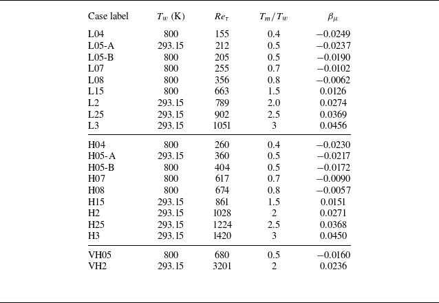
 Reτ=ρ¯wuτδc/μ¯w
 Tm/Tw
 βμ

 H05-A
 Tm/Tw=0.5
 Reτ=360
 H3
 Tm/Tw=3
 Reτ=1420

 (VFI+VFII)/TF
 H05-A
 H3
 δc

 uτ
 θτ

 yo/δc=0.4
 Reτ=640

 yo/δc=0.4
 Reτ=640

 yo/δc=0.2

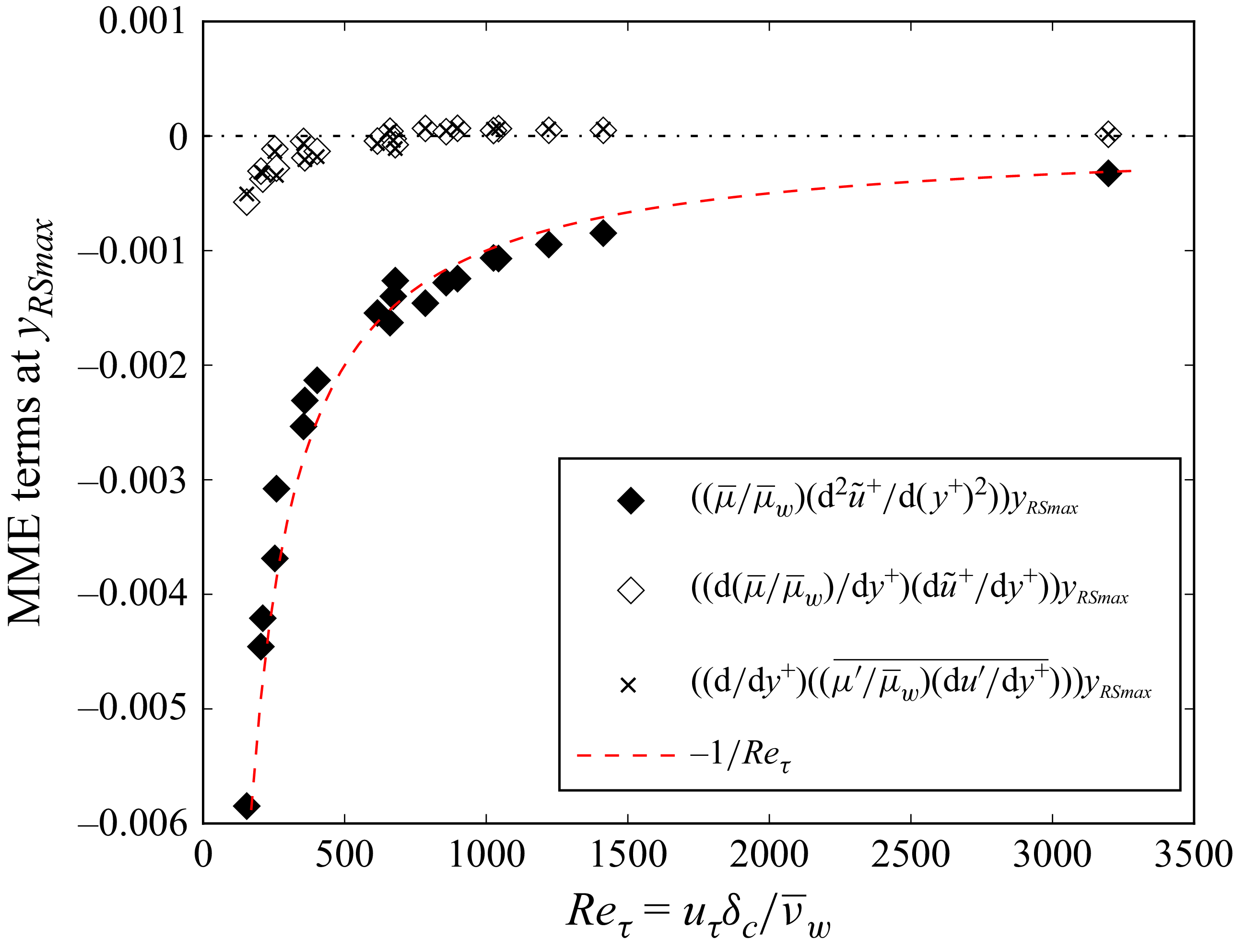
 yRSmax
 uτ
 νw/uτ

 yRSmax/δc
 Reτμ¯w/μ¯RSmax

 τw
 Reτ

 Reτ=640

 Reτ=640

 H05-A
 H2
 H05-A
 H2
 Reτ=640


 u¯
 μ¯
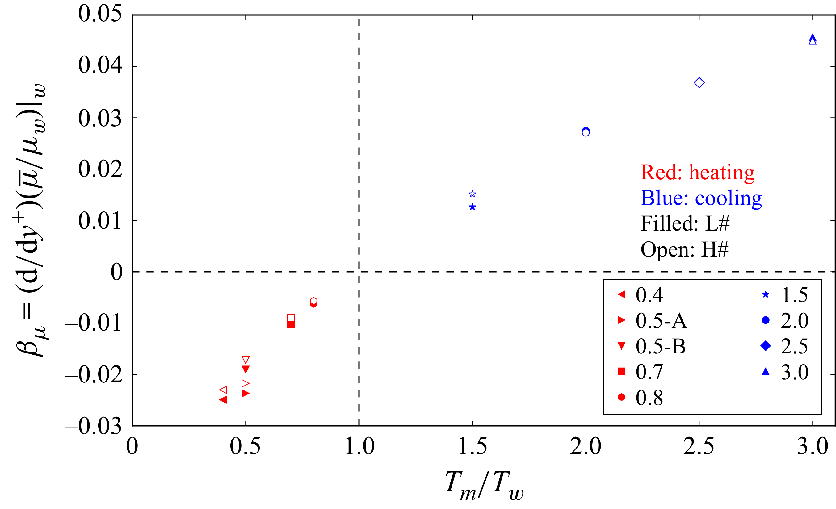
 βμ


 y−


