Investment strategies that incorporate ‘glide paths’ are widely used for pension planning. Asset classes can be roughly divided into two categories: a risky asset class, such as equity, and a less risky asset class, such as developed economy government bonds. The glide-path investment strategy typically reduces the equity proportion and increases the bond proportion in the investment portfolio as an individual approaches retirement. However, these strategies do not typically include deferred annuities (DAs) as an asset class, even though an annuity is normally an important source of a retirees' income. Annuity markets have started to give investors the freedom to use DAs. US insurance companies began selling deferred income annuities (DIA) in 2011. Currently, more than 16 insurers offer the product (Chen et al., Reference Chen, Haberman and Thomas2019). LIMRA estimates that total annuity sales in 2019 were $241.7 billion whereas DIA sales were a much smaller $2.5 billion. Academic research has paid relatively little attention to how these products can be integrated into a pre-retirement investment portfolio. The US Treasury allows target date funds to include DAs among their assets in 401(k) plans (United States Department of Treasury, 2014). Many retirement funds, however, apply more traditional, simple glide-path strategies where the allocation to the risky asset class declines as a linear function of the individual's age. In doing so, they fail to maximize an investor's utility in terms of retirement income (Merton, Reference Merton2014).
Starting with a stochastic optimal investment solution to a retirement planning problem, we calculate glide paths that include traditional asset classes – cash, bonds and equities – but which also incorporate DAs. The objective function that we specify maximizes the expected value of a sum of time-separable power utility (constant relative risk aversion, CRRA) functions expressed in terms of a secured retirement income (SRI) at retirement and a bequest before retirement. In order to solve the optimization problem, we employ multi-stage stochastic programming (MSP) which is widely used in operations research (Ziemba, Reference Ziemba2003). We then implement a strategy that averages the proportions of the optimal investment and DA allocations over time as our new glide-path strategy.Footnote 1 In particular, we extend the approach of Konicz et al. (Reference Konicz, Pisinger and Weissensteiner2016), but we focus on the accumulation phase.
There are a significant number of papers that explore the optimal choice involving immediate fixed, variable and inflation-linked annuities. Most studies focus on various types of annuity strategies only at or after retirement (i.e., in a decumulation phase). Koijen et al. (Reference Koijen, Nijman and Werker2011) present the optimal full-annuitization portfolio of fixed, inflation-indexed and variable annuities with changes in state values upon retirement and its hedging strategy in the pre-retirement period. In the hedging strategy, the optimal composition of nominal and inflation-linked bonds depends upon the annuity strategy that will be used at retirement. Also, Boulier et al. (Reference Boulier, Huang and Taillard2001), Deelstra et al. (Reference Deelstra, Grasselli and Koehl2003) and Cairns et al. (Reference Cairns, Blake and Dowd2006) show the optimal dynamic asset allocations for enhancing the utility of lifetime consumption when there is hedging demand for annuity risk.
There are fewer studies, however, that focus on the optimal investment and DA choice for an individual prior to retirement (Horneff et al., Reference Horneff, Maurer and Rogalla2010; Maurer et al., Reference Maurer, Mitchell, Rogalla and Kartashov2013; Huang et al., Reference Huang, Milevsky and Young2017). They generally assume that: the individual has an uncertain labour income stream; that the individual invests their disposal income in risk-free bonds and risky stocks; and that the individual is able to buy DAs at any time before retirement. The DAs begin to pay lifetime benefits at a fixed retirement date. The individual may also have state or defined-benefit-type pension entitlements, which pay lifetime retirement income as some function of their final salary. These studies show that DAs have a crucial role in increasing welfare gains. The optimal strategy is to start purchasing DAs early (from age 40) and to continue to purchase them over time until they comprise about 80% of the final portfolio at retirement (Horneff et al., Reference Horneff, Maurer and Rogalla2010; Maurer et al., Reference Maurer, Mitchell, Rogalla and Kartashov2013).
Huang et al. (Reference Huang, Milevsky and Young2017) consider purchases of DAs where the interest rate process is mean-reverting. DAs are, of course, expensive in the current low interest rate environment. If the interest rate process is mean-reverting, Huang et al. (Reference Huang, Milevsky and Young2017) show that a risk-neutral person should wait until the yield reaches the long-term average before buying DAs. For a risk-averse investor, there exists an entry boundary for interest rates, at which the investor begins to buy DAs. There is also an exit boundary at which the investor spends all of their remaining wealth to buy DAs. Huang et al. (Reference Huang, Milevsky and Young2017) provide an asymptotic approximation for the boundary strategy. However, no investment uncertainty and additional cash inflow is assumed, that is, there is no capital growth and no contributions from labour income.
The optimal timing for annuitization is another important decision in retirement planning. Horneff et al. (Reference Horneff, Maurer, Mitchell and Dus2008, Reference Horneff, Maurer, Mitchell and Stamos2009) investigate optimal dynamic annuitization and investment choices on immediate constant-payment annuities during the retirement period and with immediate variable-payment annuities as well as allocations to stocks and bonds prior to retirement. Buying an increasing quantity of immediate annuities (IAs) enhances the individual's welfare. The optimal equity allocation over time declines, which corresponds to the typical life-cycle pattern; the optimal bond allocation increases over time. Blake et al. (Reference Blake, Cairns and Dowd2003) examine the performance of distribution strategies using constant-payment annuities, equity-linked annuities and equity-linked income-drawdown. They note that a higher bequest motive and a larger fund size lead to a later annuitization age. Without the bequest motive, the optimal annuitization age is very sensitive to relative risk aversion. For a highly risk-averse individual, immediate annuitization is optimal.
In this paper, we adopt the general framework of these earlier studies, but we focus here on the appropriate glide-path strategy for a personal retirement plan where DA purchases are available in the accumulation phase. Using MSP, we find an optimal solution to the optimization problem and use average proportions of the optimal investment and DA allocations over time as the glide-path strategy. The investment opportunities are time-varying. Compared with simulation and dynamic programming which are widely used for solving retirement planning problems numerically, MSP enables us to incorporate sophisticated financial market models and realistic constraints, such as those on asset classes, transaction costs and taxes.
We investigate the performance of our glide paths with different fee structures and personal preferences by comparing these strategies with conventional retirement-plan strategies, such as a constant-mix, glide-path and ‘100 − age’ investment strategies. Our main contribution to the retirement planning literature in this paper is the introduction of a new, optimally-based glide path, that incorporates DAs in the accumulation phase. Our results show that this new approach is superior to traditional glide paths in terms expected retirement income per unit risk. Many retirement funds currently apply simple glide-path strategies that do not allow for the incorporation of DAs. Also, the traditional glide-path strategies fail to maximize an investor's utility in terms of retirement income.
The rest of this article is organized as follows. We describe the portfolio optimization problem, the price dynamics of available assets and the construction of our new glide paths with DAs in Section 1. In Section 2, the time-varying and predictable market movements of equity returns and yield curves are defined using a vector autoregressive (VAR) model with the Nelson–Siegel model. We solve the model by applying an MSP approach. Descriptions of the model formulation are given in Section 3. We investigate the numerical results of stochastic optimal solutions produced by the MSP approach and by the new glide paths in Section 4.
1. Investment for a retirement plan
1.1 The investment problem
We consider an individual investor who has a personal retirement plan at time 0, who is δ years of age and who retires at time T. During the retirement planning period [0, T) they contribute a fixed proportion ϕ of their labour income L t (at time t) every year to the retirement plan. The individual can hold cash, bond and equity funds in the retirement plan, which is worth W t at time t and can make withdrawals. The individual can only buy DAs which will pay out at time T (if the individual survives until this date) every year from time T until the individual's death. In our model the annuities are irreversible contracts, which means that the individual can only purchase annuities. Every unit of annuity that is bought pays out a secured income of £1 annually in retirement. If the individual dies before retirement, then the annuities do not pay out and are terminated, but the wealth in their fund is bequeathed to the individual's heirs. If they survive until retirement, then the accumulated wealth in the plan is fully annuitized to purchase an IA.
During the retirement planning period [0, T), the individual selects an asset allocation, including DAs, in order to maximize the expected utility of retirement income and of the bequest before retirement. Note that we consider investment for a retirement plan only, and therefore we assume that the individual can separate the utility from retirement income from the utility derived from pre-retirement consumption.
The individual investor has a power utility function u(t, x) = e−ρtx 1−γ/(1 − γ) in terms of cash flow or wealth x at time t. Their utility therefore has a CRRA parameter γ. As γ tends to one, the utility function becomes log utility. We assume that all retirement income is used for consumption, so that the utility function is defined in terms of the income generated by the annuities. The time impatience parameter 0 ≤ ρ ≤ 1 reflects the individual's preference for early cash flow compared to late cash flow. The utility function is also defined with regards to the bequest amount W t before retirement.
We adopt standard, actuarial notation to represent survival and death probabilities. The probability that a δ-year-old person survives until age δ + t is denoted as ${}_t^{} p_\delta$ . The probability that a person aged (δ + t) years dies over the following Δt years is denoted as ${}_{{\rm \Delta }t}^{} q_{\delta + t}$
 , abbreviated to q δ+t when Δt = 1. For practical purposes, we also assume that a person cannot live beyond age ω, which is the maximum age in an actuarial life table, so the individual investor dies before or at time τ = ω − δ, since they are δ years old at time 0.
Let the total number of units of DAs purchased by time t be X A,t, where the subscript A stands for annuities. Since each unit of annuity provides £1 annually during retirement, the SRI by time t is X A,t. If the annuity price is S A,t, then the investor pays S A,t(X A,t − X A,t−1) to buy annuities at time t ∈ [0, T] (with X A,−1 = 0).
We also assume that the investor buys and sells units or shares in a cash, bond or an equity fund, denoted C, B and E, respectively.Footnote 2 Let X B,t be the number of units of the bond fund held in the retirement plan at time t, and S B,t be the price of bond units at time t. A corresponding notation holds for the cash and equity funds. At time t, the individual decides how much to hold in cash, bonds and equities, and how many annuity units to buy. The decision variable for the individual at time t ∈ [0, T) is therefore X t = [X C,t, X B,t, X E,t, X A,t]′.
The retirement planning problem consists of the objective function, budget constraints and variable constraints given by the equation below:


In equation (1a), the decision variables over which expected utility is maximized are the portfolio and annuity purchase decisions over the planning horizon [0, T). Since the retirement income secured through DA purchases by retirement time T is X A,T, the utility of secured income at time t ∈ [T, τ) during retirement is u(t, X A,T) = e−ρt(X A,T)1−γ/(1 − γ). A bequest parameter κ captures the importance of bequest relative to retirement income. If the individual dies during period [t, t + 1), then wealth W t+1 constitutes a bequest, so that the utility of the bequest is then $\kappa ^\gamma \cdot u( {t + 1, \;W_{t + 1}} ) = \kappa ^\gamma \cdot {\rm e}^{-\rho ( {t + 1} ) }( {W_{t + 1}} ) ^{1-\gamma }/( {1-\gamma } )$ .
The budget constraint, in equation (1b), shows the dynamics of wealth W t in the retirement plan. Wealth is increased by a contribution which is a fixed proportion ϕ of labour income L t, as well as by changes in the price of the cash, bond and equity funds, (S i,t+1 − S i,t) for i = {C, B, E}. Wealth in the retirement plan is reduced if there is a withdrawal of S A,t(X A,t − X A,t−1) to buy DAs at time t.
The constraint in equation (1c) means that annuities can be bought but not sold, while the constraint in equation (1e) means that short sales are not allowed. The terminal conditions at retirement time T in equations (1d) and (1f) assert that cash, bond and equity holdings are sold, and all wealth in the retirement plan is annuitized. Equation (1g) ensures that wealth remains positive. The initial conditions in equation (1h) state that the investor has a known initial wealth and no DA at time 0.
The objective function emphasizes that income during retirement, rather than wealth at retirement, is the key variable for pensioners. This is not new in the retirement planning literature (Charupat and Milevsky, Reference Charupat and Milevsky2002; Blake et al., Reference Blake, Cairns and Dowd2003; Horneff et al., Reference Horneff, Maurer, Mitchell and Dus2008; Koijen et al., Reference Koijen, Nijman and Werker2011; Huang et al., Reference Huang, Milevsky and Young2017). The terminal wealth utility cannot measure retirement income and annuity risks properly (Merton, Reference Merton2014). Although we select income-based utility, the most ideal and practical model would be a consumption-based utility maximization model. For simplicity, we assume that the individual investor spends all of their annuity income to subsidize their consumption after retirement.
Our objective function has limitations. It is implicit in such a function that income-generating financial instruments, such as annuities, are the best financial product for retirees. If annuities are priced with a loading factor to allow for fees and expenses, they will be less appealing than other financial assets. We also assume full annuitization at retirement so that if the bequest to heirs after retirement is an important concern, the objective function would have to be modified accordingly. Similarly, if the individual has an irregular consumption pattern during retirement, or desires a high degree of liquidity, the objective function would also have to be changed to accommodate this.
1.2 Available assets
The individual can rebalance their portfolio and buy DAs at regular intervals of length Δt years. There are N ∈ ℕ such regular intervals in the retirement planning period [0, T) (i.e., T = N ⋅ Δt) (see Figure 1). Defining R i,t as the accumulated log-return of asset i ∈ {C, B, E} from time t − Δt to t, the price S i,t of asset i evolves according to the following equation:

where S i,0 = 1 without loss of generality.
Retirement planning and retirement periods from time 0 to τ.
Note: Maximum life span of an individual is denoted by τ. One increment indicates 1 year. The time length of Δt is greater than 1 year.
Source: Author's drawing.

The gross return of the long-term bond fund with a maturity of M years over a holding period of length Δt from time t − Δt to t is approximated by

The term y(β t, M, λ) denotes the M-year spot rate at time t, determined by the Nelson–Siegel term structure model, with parameters β t and λ, to be specified shortly. Accordingly, the dynamics of the bond fund price is obtained by substituting R i,t from equation (3) into equation (2).
The gross return generated by the cash fund is defined by changing the bond maturity M in equation (3) to Δt. The cash fund return from time t − Δt to t, is therefore given by

Of course, this cash fund return at time t does not depend on the current spot rate y(β t, Δt, λ) at time t, but on the past spot rate y(β t−Δt, Δt, λ).
For a policyholder aged δ + t at time t, the fair actuarial price of a DA contract paying £1 of annual retirement income for a lifetime starting at retirement at time T is

We assume static pricing mortality rates here.
1.3 Glide paths with DAs
We approximate a new glide path by averaging stochastic optimal DA and investment allocations (in percent) over the planning horizon [0, T). Let G i,t be the glide-path strategy (in percent) for asset i at time t and it is given by

The glide paths can be constructed with and without DAs.
The glide-path strategy is not an optimal investment solution to our retirement planning problem. One alternative could be to construct an optimization problem to search for an optimal glide path {G i,t} as one of the decision variables. Finding a global, or close-to-global optimal solution is a hard problem for any currently available solvers. Our new glide-path strategy can be a good starting point for searching for a better solution.
There are some practical advantages of glide-path strategies over the optimal stochastic strategy. First, they can deliver a complex investment strategy to individuals in a way which is easy for individuals to understand. If the strategy is deployed and then updated regularly, then the final retirement income derived for the glide path and optimal stochastic strategies should be the same, since they are identical at time 0.
2. Financial modelling and data
In order to incorporate interest rate uncertainty into the DA price, a stochastic term structure model is required. We choose the Nelson–Siegel model along with a VAR model for stochastic equity and bond returns.Footnote 3 This allows our model to incorporate asset return predictabilities and to use a continuous yield curve for pricing not only the cash and bond funds, but also annuities.
The entire yield curve is determined by a fitted Nelson–Siegel model with three parameters: β 1,t (level), β 2,t (slope) and β 3,t (curvature). The Nelson–Siegel model for the s-year spot rate at time t is as follows:

where the scaling parameter λ is a constant. Here, β t = [β 1,t, β 2,t, β 3,t]′.
To incorporate predictabilities of asset returns and the three parameters in the Nelson–Siegel model, we use a VAR(1) model (for details, see Barberis, Reference Barberis2000; Campbell et al., Reference Campbell, Chan and Viceira2003). In particular, a VAR model combining the interest rate model and equity returns is used, as in Ferstl and Weissensteiner (Reference Ferstl and Weissensteiner2011), Pedersen et al. (Reference Pedersen, Alex Weissensteiner and Poulsen2013) and Konicz et al. (Reference Konicz, Pisinger and Weissensteiner2016). Our VAR model is given by

where z t = [r t, β 1,t, β 2,t, β 3,t]′. Here, r t is the monthly log-returns generated by the equity fund. The accumulated return on the equity fund R E,t, defined in equation (2) as the log-return from time t − Δt to t, is simply a sum of the monthly log-returns. In equation (8), Φ0 is a column vector of intercepts, Φ1 is a 4 × 4 matrix of the slope coefficients of the VAR model, and v t is a column vector of iid innovations ~N(0, Σz), where Σz = $\opf E$ [vv ′].Footnote 4
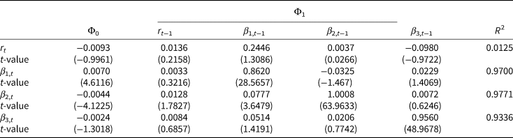
We use monthly yield curve data calculated by the Bank of England with 0.5 to 25-year spot rates, and returns generated by the FTSE 100 collected from the Bloomberg from January 1993 to December 2013. By minimizing the sum of squared errors between the fitted and historical yield curves, we estimate λ = 0.382 in equation (7). Our estimates for Φ0 and Φ1 in equation (8), along with t-statistics, are presented in Table 1. The level of R 2 for the equity equation is low, making it difficult to confirm that return predictability in the UK equity market exists. The eigenvalues of Φ1 have moduli less than one, so that the unconditional expected mean and covariance in equations (9) and (10) exist. Table 2 presents the correlations and standard deviation (multiplied by 100) of the residuals. Table 3 presents the unconditional expected mean μ zz of z t.
VAR(1) parameters and t-statistics

Note: The scale parameter of a Nelson–Siegel term structure model is set to λ = 0.3820; t-statistics in parenthesis.
Source: Author's calculations using monthly data of FTSE 100 from Bloomberg and fitted yield curves from the Bank of England from January 1993 to December 2013.
Cross correlations and standard deviations of residuals of the VAR(1) model

a Standard deviations along the leading diagonal are multiplied by 100.
Source: Author's calculations using monthly data of FTSE 100 from Bloomberg and fitted yield curves from the Bank of England from January 1993 to December 2013.
Unconditional expected mean for the steady state of the VAR(1) model

Source: Author's calculations using monthly data of FTSE 100 from Bloomberg and fitted yield curves from the Bank of England from January 1993 to December 2013.
3. MSP formulation
3.1 Scenario generation
An MSP model can be constructed in a nodal form by using state variables generated in a scenario tree. The scenario tree starts at the initial stage from a unique root node which branches out to several ‘children’ nodes at the second time stage. Each of these child nodes themselves branch out to further nodes at the third time stage, and so on. The nodes at the terminal stage are known as leaf nodes. A scenario is the path followed from the root node through descendant nodes to a leaf node. The tree is non-recombining. Some helpful notation pertaining to the scenario tree and the scale of the optimization problem formulated here is set out in Appendix A.
3.2 The optimization problem
The objective function and constraints set out in equation (1) for the general problem can now be formulated within the scenario tree as an MSP problem. The notation transfers in a straightforward way, except that we index by node rather than by time. For example, X i,n refers to the number of units of asset i ∈ {C, B, E, A} held at node n in the scenario tree. We also distinguish between buy and sell decisions, so that $X_{i, n}^{buy}$ is the number of units of asset i to buy at node n and $X_{i, n}^{sell}$
 is the number of units of asset i to sell at node n. Recalling that DAs cannot be sold, the decision variable for the individual at node n is therefore $X_n = [ {X_{C, n}^{buy} , \;\;\;X_{C, n}^{sell} , \;\;\;X_{B, n}^{buy} , \;\;\;X_{B, n}^{sell} , \;\;\;X_{E, n}^{buy} , \;\;\;X_{E, n}^{sell} , \;\;\;X_{A, n}^{buy} } ] ^{\prime}$
 for $n\in {\cal N}$
 .
The objective function in equation (1a) is rewritten in a nodal form as follows:

where it is implicit that summations occur over the time stages in the scenario tree during the planning phase when t ∈ [0, T].
A cash balance constraint, shown in equation (10), controls cash inflows and outflows. Below $\varphi _i^s$ and $\varphi _i^u$
 indicate a percentage selling fee and upfront fee respectively for asset i ∈ {C, B, E, A} and w 0 represents non-random, positive initial wealth:

An asset inventory constraint shown in equation (11) tracks the number X i,n of units of asset i ∈ {C, B, E, A} held at node n. Below $\varphi _i^m$ indicates a percentage management fee for asset i:

Wealth in the retirement plan, which includes cash, bond and equity funds, and excludes purchased DAs, satisfies the following equations:

Variable constraints appear below and complete the MSP formulation which is equivalent to the general optimization problem in equation (1):


The terminal condition in equation (1d) is self-constrained through equations (10), (11) and (13). The non-negative wealth condition of equation (1g) is not imposed because it is satisfied in equation (12) since asset prices are positive and no short-selling is allowed in equations (11) and (13a). Wealth is initialized at the non-random amount w 0 specified on the l.h.s. of equation (10).
Following equation (10) to equation (13), on every node in the scenario tree, the cash balance, asset inventory and other constraints are set. Finally, we use an interior point solver MOSEK to find optimal investment and DA choices by maximizing the non-linear objective function in equation (9) subject to the linear constraints in equations (10) to (13). Hilli et al. (Reference Hilli, Koivu, Pennanen and Ranne2006), Konicz and Mulvey (Reference Konicz and Mulvey2015) and Konicz et al. (Reference Konicz, Pisinger and Weissensteiner2016) use the MOSEK for pension asset-liability management and financial planning applications.
4. Results
4.1 Numerical examples
We start with a benchmark case in which a 40-year-old individual (δ = 40) intends to retire at age 65 (T = 25). Their goal is to maximize and secure their retirement benefits in nominal terms and to set aside a portion of the portfolio as a bequest in the event of them dying before retirement. In their retirement plan they can invest in a cash fund (maturity M = 5 years), a bond fund (maturity M = 20 years), an equity fund and in DAs as described earlier. To price the DA, we use a UK mortality table based on 2000–2006 experience.Footnote 5
The individual can rebalance the portfolio and buy DAs every 5 years (Δt = 5) so there are six stages (five periods) in the scenario tree spanning the 25-year planning horizon. The individual has an initial wealth of $w_0 =$ £80, 000 which represents the initial value of the retirement plan. Annual wage is fixed at £40,000 throughout.Footnote 6 Contributions to the retirement plan are £4,000 p.a. (ϕ = 10%). Because of the incidence of cash flows in our model, the contribution is, in effect, £20,000 every 5 years in advance ($\phi \cdot L_n\cdot {\rm \Delta }t = \pounds20, \;000$
 for $n\in {\rm {\cal N}\backslash }{\cal N}_T$
 ).
In the benchmark case, the individual is a male with risk aversion coefficient γ = 3, time preference ρ = 0 and bequest parameter κ = 0. For the bond and equity funds, upfront and selling fees are $\varphi _i^u = \varphi _i^s = 0.5\percnt$ for i ∈ {B, E}, following Geyer et al. (Reference Geyer, Hanke and Weissensteiner2009) and Konicz et al. (Reference Konicz, Pisinger, Rasmussen and Steffensen2014). Expense loadings on annuities are $\varphi _A^u = 3.0\percnt$
 . This is a similar level to the one used by Horneff et al. (Reference Horneff, Maurer and Rogalla2010) and Huang et al. (Reference Huang, Milevsky and Young2017). The cash fund has no fees, and management fees for all assets are ignored. Alternative cases are also considered with different individual preference parameters and transaction costs.
We also consider three different fee structures from the benchmark, which we denote case I. A higher fee on bond and equity transactions from 0.5 to 1.0% but the same loading as the benchmark case, is referred to as case II. Although case III uses a higher loading on annuities of 5.0%, but the same transaction fee as in the benchmark case. Case IV increases both transaction fees and loading to 1.0% and 5.0%, respectively.
To control the glide-path operation within scenarios we should take transaction fees into account, so that after-rebalancing asset proportions match the target glide-path strategy G i,t. Let $\tilde{G}_{i, n}$ be the current proportion of asset i ∈ {C, B, E, A} at node n before rebalancing but after making the contribution ϕ ⋅ L n into the cash account. We rebalance asset allocations from $\tilde{G}_{i, n}$
 to G i,t after fees at every node $n\in {\rm {\cal N}\backslash }{\cal N}_T$
 . The total transaction and loading costs denoting fee n are calculated by

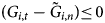
where a function sign(i) returns +1 when $( {G_{i, t}-{\tilde{G}}_{i, n}} ) > 0$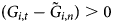 and −1 when $( {G_{i, t}-{\tilde{G}}_{i, n}} ) {\rm \leq }\,0$
 . If $G_{i, t} = \tilde{G}_{i, n}$
 for all i ∈ {C, B, E, A}, then no fees occur since rebalancing is not required. Management fees are ignored, but it is not non-trivial. If the current proportion of DA to wealth plus contribution is greater than that in the glide path, we do not change the DA allocation (X A,n is equal to $X_{A, n^-}$
 ) and calculate the total transaction cost in equation (14), excluding the DA. In that case, G i,t and $\tilde{G}_{i, n}$
 are adjusted by considering only assets i ∈ {C, B, E} as one portfolio and W n deducted by $S_{A, n}X_{A, n^-}$
 in equation (14).
4.2 Traditional glide-path strategies
We consider two traditional glide paths. The ‘equity-to-bond’ glide-path starts with 80% in equities, a proportion that falls by 6% points every 5 years, with the proportion invested in bonds rising commensurately. The ‘equity-to-cash’ glide-path also starts with 80% in equities, a proportion that falls by 6 percentage points every 5 years, with the proportion invested in cash rising commensurately. The equity allocations in the traditional glide-path strategies match those suggested by Vanguard (Daga et al., Reference Daga, Schlanger, Donaldson and Westaway2016).
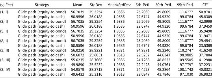
Table 4 presents basic statistics for the retirement income secured by the representative individual for a range of the risk aversion parameters, γ, (1, 3, 5 and 8) and the fee structures of cases I, II, III and IV. The first column indicates the risk aversion parameter and fee structure for each row. The first row for each pair shows the results for the strategy where the investor applies the equity-to-bond glide-path strategy and purchases an IA at retirement. The second row shows equivalent statistics, but where the individual implements the equity-to-cash glide path, etc.
SRI (£1,000 p.a.) with traditional glide-paths strategies

a Certainty equivalent values (£1,000 p.a.) to the expected utility of total SRI at retirement is achieved by solving u −1($\opf E$ [u(T, X A,T)]) = CE; ρ is ignored.
Note: Time preference and bequest coefficients are ρ = 0.0 and κ = 0.0 respectively. Upfront and selling fees are 0.0% for the cash fund and 0.5% for the bond and equity funds. Expense loadings on annuities are 3.0%. Management fees are ignored.
Source: Author's calculations.
Distributional properties from the mean to 95th percentile values of the retirement income are identical for the (1, I), (3, II), (5, III) and (8, IV) cases because the strategies do not depend on the individual's risk preference, but are identical and deterministic. The equity-to-bond strategy shows a higher mean value, but also has a higher standard deviation (StdDev) than the equity-to-cash strategy. This causes a lower expected retirement income per unit of risk (mean/StdDev) so that we cannot say that the equity-to-bond strategy is more efficient than the equity-to-cash strategy.
The last column shows the certainty equivalent value of retirement income (CE) to the expected utility of the retirement income at retirement. The equity-to-bond strategy produces a higher CE value than the equity-to-cash strategy, since investing in the bond with a 20-year maturity is less risky than investing in cash (5-year zero bond) in terms of a price change in one unit of retirement income (i.e., IA price). In addition, the CE values depend upon each individual's risk preference, although the retirement income has the same distribution in both cases. A glide-path strategy can be less valuable to a more risk-averse investor. The CE value of the retirement income ranges between about £4,000 and 6,000 per year. In all four fee cases, I to IV, CE values are lower when transaction fees or expense loading on the annuity are higher. Results with Monte Carlo simulation in Table B.2 also show similarly consistent results.
4.3 Optimal stochastic strategies
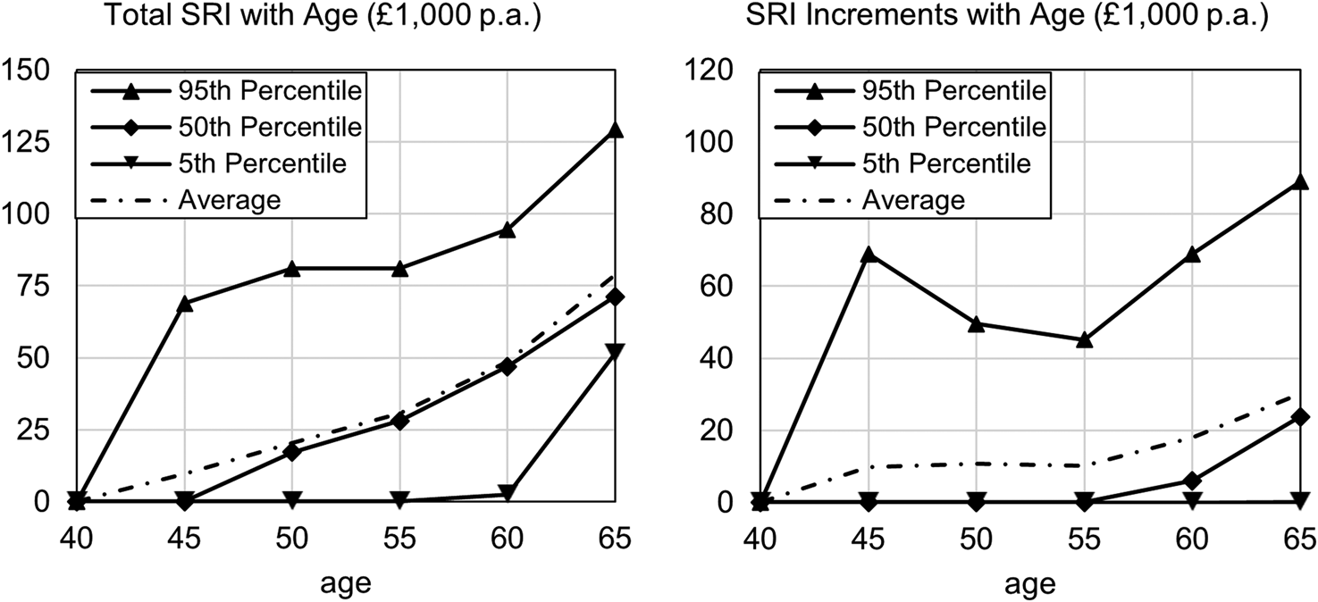
The stochastic investment strategy that results from solving the MSP problem, utilizes full information about the realized and expected values of the predictable and time-varying financial variables (for details, see Owadally et al., Reference Owadally, Jang and Clare2021). Figure 2 shows the percentiles and average of the total optimally SRI generated by employing the MSP approach for the benchmark model, as a function of age. The left panel of Figure 2 shows the total SRI. The right panel shows the extra retirement income gained by purchasing DAs. This benchmark case shows that the optimal strategy to secure retirement income involves buying DAs regularly during the individual's working lifetime, starting fairly early and accelerating in the last years before retirement. The result is robust for other investor profiles. Supplementary results are presented with different risk aversion, time preference and bequest parameters in following sections and in Table B.1.
Percentiles and average of optimally SRI in total (left) and increments (right).
Note: CRRA, time preference and bequest parameters are γ = 3.0, ρ = 0.0, and κ = 0.0, respectively. Upfront and selling fees are 0.0% for the cash fund and 0.5% for the bond and equity funds. Expense loadings on annuities are 3.0%. Management fees are ignored.
Source: Author's calculations.

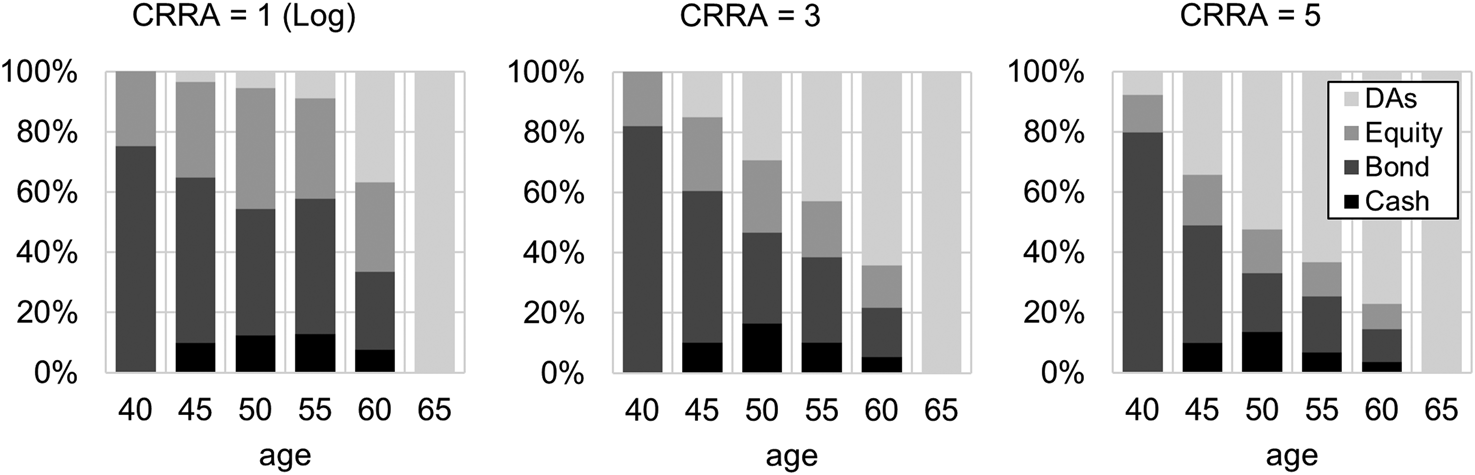
Average optimal asset allocations over the 25-year planning horizon are presented in Figure 3. The bar graphs show average asset allocations including DAs for three different CRRA parameters. The chart corresponding to CRRA = 3 shows the asset allocation for the benchmark case. The proportion of DA holding in overall wealth increases on average, as retirement approaches, while bond and equity holdings decline. The fall in equity holdings over time is consistent with findings in the lifetime finance literature and the typical recommendations of financial advisors. Bonds clearly play a significant role in the investor's portfolio. As well as being a relatively ‘safe asset class’, they also represent a partial hedge against the future price changes of DAs.
Optimal investment and DA allocations on average over the 25-year retirement planning period.
Note: CRRA, time preference, and bequest parameters are γ = {1.0, 3.0, 5.0}, ρ = 0.0, and κ = 0.0, respectively. Upfront and selling fees are 0.0% for the cash fund and 0.5% for the bond and equity funds. Expense loadings on annuities are 3.0%. Management fees are ignored.
Source: Author's calculations.

Bonds are the largest asset holdings among cash, bond and equity funds over the planning horizon, but the hedging demand seems weaker as retirement draws closer. Cairns et al. (Reference Cairns, Blake and Dowd2006) and Koijen et al. (Reference Koijen, Nijman and Werker2011) find an opposite hedging pattern using a bond, which shows that the hedging demand is stronger as retirement draws closer. They, however, do not consider DAs so that the individual has no means of securing their retirement income in advance.
The optimal allocation to the cash fund increases initially and then declines. The cash account provides liquidity for future DA purchases, especially when bond and equity prices are low.
Figures 2 and 3 demonstrate that there is a potentially important role for DAs in the accumulation phase. To see just how important, we can compare these results to those where we exclude DAs from the asset allocation choice where we instead only allow the investor to purchase an IA at retirement.
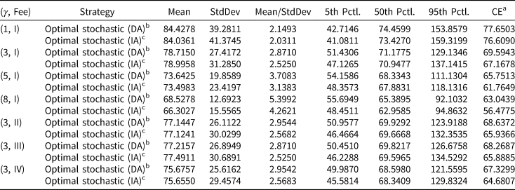
Table 5 presents statistics equivalent to those in Table 4, but for optimal stochastic strategies with DA and with IA. The first row for each pair of risk aversion level and fee structure shows the results for the strategy where the investor can purchase a DA. The second row shows equivalent statistics but where the individual is restricted to an IA only. In each case the difference between the retirement income mean is economically small. However, for each level of γ the individual achieves higher expected retirement income per unit risk (mean/StdDev) when DAs are available compared to when they are not. The last column, ‘CE’, shows that the certainty equivalent values of retirement income are also higher when DAs are available in all cases. The analysis shows that the availability of DAs provides the individual with not only a higher welfare value, but also a more efficient (higher mean-variance) retirement-income distribution.
SRI (£1,000 p.a.) with optimal stochastic strategies

a Certainty equivalent values (£1,000 p.a.) to the expected utility of total SRI at retirement is achieved by solving u −1($\opf E$ [u(T, X A,T)]) = CE; ρ is ignored.
b This strategy is resulted from the MSP model. DAs are available at any time before retirement and IAs are available only at retirement.
c This strategy is resulted from the MSP model. DAs are not available and IAs are only available at retirement.
Note: Time preference and bequest coefficients are ρ = 0.0 and κ = 0.0 respectively. Upfront and selling fees are 0.0% for the cash fund and 0.5% for the bond and equity funds. Expense loadings on annuities are 3.0%. Management fees are ignored.
Source: Author's calculations.
Comparing Table 5 with Table 4, we find that the optimal stochastic strategies produce more efficient retirement income distributions (i.e., higher mean/StdDev values) and higher certainty equivalent value in all cases. The differences in the certainty equivalent values are particularly large, about £26,000 to £34,000 per year, which grow with the risk aversion parameter.
4.4 A glide-path approach with DAs
Implementing the optimal stochastic strategy, however, is likely to be too complex for individual investors or their advisors to understand. To this end, we now introduce an investment glide path. The glide path G i,t, described in equation (6), defines the proportion of asset i in the retirement plan, including a proportion in a DA as a function of time. It can be written in the following nodal form:

Our numerical results show that this glide-path guarantees a better welfare value in terms of certainty equivalent retirement income than traditional glide paths, constant-mix investment and ‘100 − age’ strategies, which are widely used in the retirement planning industry.
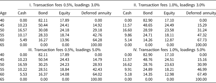
Table 6 shows that the outcomes delivered with the introduction of G i,t (in percent) with different transaction costs on bond and equity funds and expense loadings on DAs. All average portfolio allocations are calculated after fees as in equation (6). When the expense loading increases by 2.0% to 5.0% (see I and III or II and IV panels), the glide path lowers DA proportions through the planning horizon. When transaction costs (upfront and selling fees) on bond and equity funds increase by 0.5% to 1.0% (see I and II or III and IV panels), the new glide-path results show higher DA proportions and lower other proportions in other asset classes through the planning horizon. When the fees on bond and equity funds increase, cash fund allocations increase through the planning period because transaction fees on the cash fund are set to zero.
New glide-path strategies (%) with transaction costs and loadings

Note: The four columns in panels I–IV indicate averages of the optimal investment and DA portfolio allocations (%) for the 25-year planning horizon. From the first column, cash, bond, equity funds and DAs at the given age. The averages are expected values of 15,552 scenarios. CRRA, time preference and bequest coefficients are γ = 3.0, ρ = 0.0, and κ = 0.0, respectively. Management fees are ignored.
Source: Author's calculations.
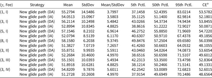
The results in Table 7 with Tables 4 and 5 demonstrate that the introduction of G i,t produces the most efficient distribution of retirement income and a higher certainty equivalent value of retirement income than traditional glide-path strategies. The mean/StdDev values are much higher than the stochastic optimal strategies. The difference in the certainty equivalent values between the traditional and new glide path is about £3,000 to 12,000 per year. A more risk-averse individual is likely to see a larger difference in the certainty equivalent value. A certainty equivalent gap between the new glide path and the optimal stochastic strategies decreases as the individual becomes more risk averse.
SRI (£1,000 p.a.) with new glide-path strategies

a Certainty equivalent values (£1,000 p.a.) to the expected utility of total SRI at retirement is achieved by solving u −1($\opf E$ [u(T, X A,T)]) = CE; ρ is ignored.
Note: Time preference and bequest coefficients are ρ = 0.0 and κ = 0.0 respectively. Upfront and selling fees are 0.0% for the cash fund and 0.5% for the bond and equity funds. Expense loadings on annuities are 3.0%. Management fees are ignored.
Source: Author's calculations.
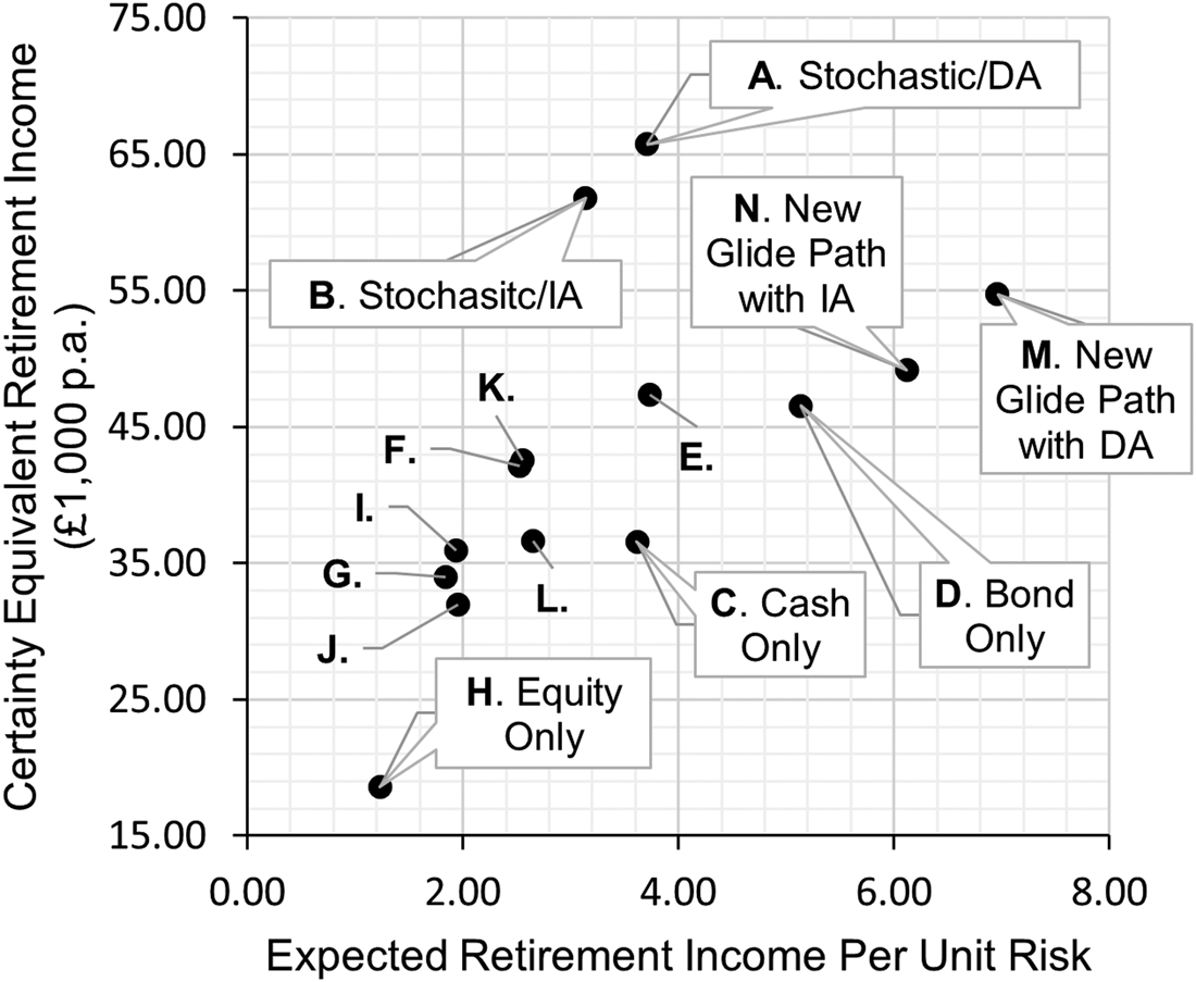
It is also helpful to compare our glide-path strategies with other deterministic strategies used in practice. We measure two performance metrics: the expected retirement income per unit risk and the certainty equivalent retirement income. This is done for 14 different strategies and the results are displayed in Figure 4. The 14 strategies labelled in Figure 4 are as follows:
-
(A) stochastic optimal strategy with deferred annuities (DA) available including an immediate annuity (IA) at retirement;
-
(B) stochastic optimal strategy without DAs but including an IA at retirement;
-
(C) cash only;
-
(D) bond only;
-
(E) 70/30 bond/equity;
-
(F) 50/50 bond/equity;
-
(G) 30/70 bond/equity;
-
(H) equity only;
-
(I) glide path starting from 80/20 equity/bond with equity decreasing and bond increasing by 6 percentage points every 5 years;
-
(J) glide path starting from 80/20 equity/cash with equity decreasing and cash increasing by 6 percentage points every 5 years;
-
(K) (100 − age) percent in equity and the rest in bond;
-
(L) (100− age) percent equity and the rest in cash;
-
(M) glide-path strategy with DA available including an IA at retirement; and
-
(N) glide-path strategy without DAs, but including an IA at retirement.
Certainty equivalent retirement income (£1,000 p.a.) and expected retirement income per unit risk for various investment strategies.
Note: CRRA, time preference, and bequest parameters are γ = 5.0, ρ = 0.0, and κ = 0.0, respectively. Upfront and selling fees are 0.0% for the cash fund and 0.5% for the bond and equity funds. Expense loadings on annuities are 3.0%. Management fees are ignored.
Source: Author's calculations.

Figure 4 shows that our glide paths with and without DAs ((M) and (N) have a better performance than any of the deterministic investment strategies ((C) to (L)) in terms of the expected retirement income per unit risk. For the certainty equivalent retirement income our new glide path performs better than the typical glide-path strategies ((I) to (J)), but also better than any constant-mix strategies ((C) to (H)) and ‘age − 100’ strategies ((K) and (L)). The stochastic optimal strategies ((A) and (B)) clearly show the highest certainty equivalent retirement income. Strategy (H) (equity only) has the worst performance among the fourteen strategies, under both performance metrics.
5. Conclusions
Using MSP, we specify an optimization model with the objective function to maximize the expected value of a series of power utility functions of SRI from purchased annuities at retirement and a bequest before retirement. Then we propose and construct new glide paths by averaging optimal stochastic asset allocations which are achieved by solving the retirement planning problem. The MSP approach enables us to incorporate sophisticated financial market models and realistic constraints, such as constraints on assets, transaction costs and taxes.
Numerical results show that our glide-path strategies provide the individual with a higher welfare value, and a more efficient investment portfolio than any conventional deterministic strategies, such as constant-mix, traditional glide-path and ‘100 − age’ investment strategies. The new glide-path strategies also make retirement income and wealth more responsive to personal preferences: risk aversion, time impatience and bequest motive.
The welfare value is determined by the certainty equivalent value of the expected utility of SRI. The welfare value gap between our glide paths and the deterministic strategies widens as the investor is more risk-averse. The expected retirement income per unit risk, as a measure of efficiency, is the highest. Ours also show that the closer-to-optimal certainty equivalent values of the expected utility of bequest over the planning horizon. The existence of a bequest motive results in more allocations to the cash fund and delayed, or lower allocations to DAs. The findings are robust to different fee structures and to the availability of DAs.
The glide-path strategy is not an optimal investment solution to our retirement planning problem. However, there is one clear, practical advantage of the glide-path strategy over the optimal stochastic strategy: it would be easier to explain the idea to individual investors, since the new glide-path strategy is simply a deterministic function of time. Furthermore, if the glide path is updated regularly, the results from the glide path and optimal stochastic strategies will not be very different. This is because their strategies are identical at the time they are updated.
Our glide-path strategies have limitations. The model assumes full annuitization at retirement. This implies that annuities are the best income-generating financial instrument. It would have to be modified if the individual wishes to make bequest to heirs after retirement, if the post retirement consumption pattern is irregular or if a higher degree of liquidity during retirement is required.
We have not taken account of inflation rates which affect consumer prices, housing assets and wages. Uncertainties in labour income, labour supply and fiscal policy issues are also ignored. Various types of annuity products, such as index-linked annuities, are not covered. Term assurance and health insurance covering long-term care and critical illnesses are also not considered here. They can affect the optimal retirement planning and our glide-path strategy. The results that we have here are influenced by the discretization of state and time in an MSP model. In practice, individuals may wish to rebalance their portfolios more often. These limitations will be carefully investigated in our future studies.
Supplementary material
The supplementary material for this article can be found at https://doi.org/10.1017/S1474747221000251.