1 Introduction
The observation of patterns arising from resonance may be traced to Faraday (Reference Faraday1831), who used a violin bow to excite the patterns via acoustic waves in sand and in fluid mixtures. These patterns typically appear subharmonic to the forcing frequency (Rayleigh Reference Rayleigh1883), and arise either in the form of standing waves or subcritical break-up of an interface (Douady Reference Douady1990). Many resulting waveforms can be generated by controlling the system parameters, including triangular, hexagonal, square or striped structures (Müller Reference Müller1993; Edwards & Fauve Reference Edwards and Fauve1994; Kudrolli & Gollub Reference Kudrolli and Gollub1996), or discretized competing waveforms (Ciliberto & Gollub Reference Ciliberto and Gollub1985; Batson, Zoueshtiagh & Narayanan Reference Batson, Zoueshtiagh and Narayanan2013b ). As the instability itself arises from resonance, it can be excited by a variety of methods including mechanical forcing (Benjamin & Ursell Reference Benjamin and Ursell1954; Kumar & Tuckerman Reference Kumar and Tuckerman1994), acoustic forcing (Boukra et al. Reference Boukra, Cartellier, Ducasse, Gajan, Lalo, Noel and Strzelecki2009; Tsai & Tsai Reference Tsai and Tsai2013; Tsai et al. Reference Tsai, Mao, Tsai, Shahverdi, Zhu, Lin, Hsu, Boss, Brenner, Mahon and Smaldone2017) or even electrostatic forcing (Taylor & McEwan Reference Taylor and McEwan1965; Briskman & Shaidurov Reference Briskman and Shaidurov1968; Yih Reference Yih1968).
The early theoretical work of Benjamin & Ursell (Reference Benjamin and Ursell1954) demonstrated that a Mathieu equation would result when a two-fluid inviscid bilayer is subjected to mechanical oscillations. It was shown that the zones of stability alternate between subharmonic and harmonic responses. Early experiments, such as those by Abramson, Dodge & Kana (Reference Abramson, Dodge and Kana1965), Henderson & Miles (Reference Henderson and Miles1990) and Tipton & Mullin (Reference Tipton and Mullin2004) utilized this model with relative success, by accounting for viscosity through the use of additional ad hoc damping terms. Troyon & Gruber (Reference Troyon and Gruber1971) theoretically investigated the stabilization of the Rayleigh–Taylor instability by imposing oscillatory forcing akin to that imposed for the Faraday instability using a viscous model, which supported previous work by Wolf (Reference Wolf1970). Sterman-Cohen, Bestehorn & Oron (Reference Sterman-Cohen, Bestehorn and Oron2017) previously conducted a similar analysis for vertically and horizontally oscillated Rayleigh–Taylor unstable thin films in the long-wave limit. Jacqmin & Duval (Reference Jacqmin and Duval1988) further developed the viscous theoretical model for the mechanically forced Faraday instability by utilizing the Navier–Stokes equations in the absence of a mean gravitational acceleration. Kumar & Tuckerman (Reference Kumar and Tuckerman1994) developed a similar model which allowed for non-zero mean gravitational acceleration. This model was validated experimentally with great success by Bechhoefer et al. (Reference Bechhoefer, Ego, Manneville and Johnson1995) for the minimum thresholds in large geometries and by Batson et al. (Reference Batson, Zoueshtiagh and Narayanan2013b ) for finite geometries allowing discretized modes through careful fluid selection and experimental procedures. Cerda & Tirapegui (Reference Cerda and Tirapegui1998) further explored the effects of viscosity on the mechanical system in order to delineate the mechanism for the production of standing waves in highly viscous systems.
Although research on the mechanically forced Faraday instability has been extensive, studies on promoting the instability through electrostatic forcing are less common. The first models for this method of forcing were produced by Taylor & McEwan (Reference Taylor and McEwan1965), Briskman & Shaidurov (Reference Briskman and Shaidurov1968) and Yih (Reference Yih1968). These models are the electrostatic analogues to the Benjamin & Ursell (Reference Benjamin and Ursell1954) model for mechanically forced systems. Simplifying assumptions were made such as inviscid fluids and a perfect conductor–perfect dielectric pair, ultimately resulting, again, in a Mathieu equation. Bandopadhyay & Hardt (Reference Bandopadhyay and Hardt2017) recently extended these types of models to account for viscous effects. Early experiments were conducted by Devitt & Melcher (Reference Devitt and Melcher1965) utilizing high frequency fields to determine the stability thresholds between a dielectric fluid and air to great success. Iino, Suzuki & Ikushima (Reference Iino, Suzuki and Ikushima1985) and, more recently, Tsukahara, Tsuruta & Fujiwara (Reference Tsukahara, Tsuruta and Fujiwara2013) intentionally excited Faraday waves using electrostatic oscillations in laterally constrained bilayer systems to correlate the observed resonant frequencies to the interfacial tension between the fluids. The aim of these works was not to predict or measure the stability threshold, but to experimentally determine resonant frequencies for a fixed forcing amplitude of the oscillatory voltage. Pontiga & Castellanos (Reference Pontiga and Castellanos1994) and Smorodin & Taraut (Reference Smorodin and Taraut2010) have studied the effect of alternating electric fields on buoyancy convection problems. Khorshidi, Jalaal & Esmaeilzadeh (Reference Khorshidi, Jalaal and Esmaeilzadeh2011) have experimentally studied the use of constant electric fields to induce mixing between leaky dielectric fluids, and Ozen et al. (Reference Ozen, Aubry, Papageorgiou and Petropoulos2006) have performed the linear stability analysis for a Poiseuille flow of two leaky dielectric fluids in the presence of a constant electric field.
The importance of charge accumulation on the interfaces between fluids is common to all of these research studies, and the accepted theoretical model for its description is the leaky dielectric model, initially given by Taylor (Reference Taylor1966) and later presented by Melcher & Taylor (Reference Melcher and Taylor1969). This model is discussed extensively and applied to multiple problems in the review article by Saville (Reference Saville1997). In short, the model is comprised of the typical equations of motion coupled with electromechanical stresses at the fluid interfaces resulting from an accumulation of charge, allowing for departure from the stresses that arrive in perfect conductor or perfect dielectric models. This model has been used extensively to investigate and explain various electrohydrodynamic phenomena (Pease & Russel Reference Pease and Russel2002; Reddy & Esmaeeli Reference Reddy and Esmaeeli2009; Yang, Li & Xu Reference Yang, Li and Xu2017).
Most relevant to the current study is the work of Pease & Russel (Reference Pease and Russel2002) who conducted a linear stability analysis on a thin polymer film between two substrates with an air gap between the film and top substrate using the leaky dielectric model. The goal of the work was to delineate the mechanism for self-assembly patterns generated in lithography processes, where electrical fields arise naturally within the problem. Purposefully imposing a constant electric field can produce similar patterns, as shown, for example, by Dong, de Almeida & Tsouris (Reference Dong, de Almeida and Tsouris2001), Shankar & Sharma (Reference Shankar and Sharma2004), Craster & Matar (Reference Craster and Matar2005) and Tseluiko & Papageorgiou (Reference Tseluiko and Papageorgiou2007). The effect of imposing an alternating electric field was examined by Roberts & Kumar (Reference Roberts and Kumar2009, Reference Roberts and Kumar2010), who utilized the leaky dielectric model to investigate the additional control gained by employing AC fields over pillaring instabilities in thin polymer films by performing nonlinear simulations in the long-wave limit. These works effectively show that AC fields can be used to further tailor topographical expressions arising due to electrohydrodynamics for two and three-fluid films. The effect of viscoelasticity on this instability was later explored by Espin, Corbett & Kumar (Reference Espin, Corbett and Kumar2013) for both AC and DC fields. Gambhire & Thaokar (Reference Gambhire and Thaokar2010, Reference Gambhire and Thaokar2012) also utilized linear stability analysis to study the effect of alternating electric fields on the system stability in leaky dielectric bilayers of infinite lateral and axial extent and also examine the role of conductivity on the resulting instabilities both theoretically and experimentally in the thin-film limit. These works disregard inertia in their analyses and Faraday resonance is not included in the physics. The stability of thin films in these studies relates to the effect of imposed electric fields, steady and periodic, on the Rayleigh–Taylor instability. The current work is focused on resonant instability and relaxes the thin-film assumptions so as to make it applicable to experiments of interest in this study.
Much as the work by Kumar & Tuckerman (Reference Kumar and Tuckerman1994) served to improve the Benjamin & Ursell (Reference Benjamin and Ursell1954) model, this paper focuses on enhancing the Yih (Reference Yih1968) type models for electrostatically forced Faraday instability through the addition of viscosity and leaky dielectric properties for the fluids. The first aim of the current work is to introduce and explain a broad, rigorous model derived through linear stability analysis of the electrohydrodynamical equations for the prediction of purely electrostatically forced Faraday instability in two-fluid systems. The second aim is to provide experimental verification of this resonant instability. However, before introducing leaky dielectrics into the problem, we present a simpler derivation which is equivalent to an earlier model (Bandopadhyay & Hardt Reference Bandopadhyay and Hardt2017) where the inviscid assumption alone is relaxed to highlight viscous effects. The derivation for the full model with the leaky dielectric and charge dynamics is then presented. This full model is complemented by experiments that were specifically designed to allow for the validation of the model. This study therefore represents the first attempt to have a realistic model on electrostatic resonant interfacial instability. It is also the first that provides clear experimental verification and validation of resonant forcing. An important outcome of the validating experiments is a novel way to measure the interfacial tension between fluids that may be subject to electrostatic forcing. One possible application of this new technique could be the measurement of interfacial tension between semiconductors and encapsulants, such as gallium arsenide and boron oxide.
2 Theoretical models and calculations
Two sequential models are developed for the prediction of electrostatically forced Faraday instability thresholds. The first of these models is called the perfect conductor model, and is essentially an extension of the inviscid model derived by Yih (Reference Yih1968) (cf. appendix A for a re-derivation of the Yih model) to account for viscous effects. This model was also utilized in the recent work by Bandopadhyay & Hardt (Reference Bandopadhyay and Hardt2017), but is re-derived here in order to set the stage for the second more practically relevant model – one that includes charge dynamics at the interface and one that can be verified by experiments. The second model is called the leaky dielectric model and will be addressed in § 2.3. In the first model, the bottom fluid is taken to be a perfect conductor and the top fluid is taken to be a perfect dielectric. These assumptions greatly simplify the governing equations and allow for a simpler calculation due to the inherent decoupling of the perturbed voltage profiles with the perturbed hydrodynamic equations. We first present this simpler model to highlight the effect of viscosity on the instability thresholds. We then discuss the leaky dielectric model, in which both fluids are taken to be leaky dielectrics. The differences between the two models are described in the discussion of the second case.
2.1 Perfect conductor model
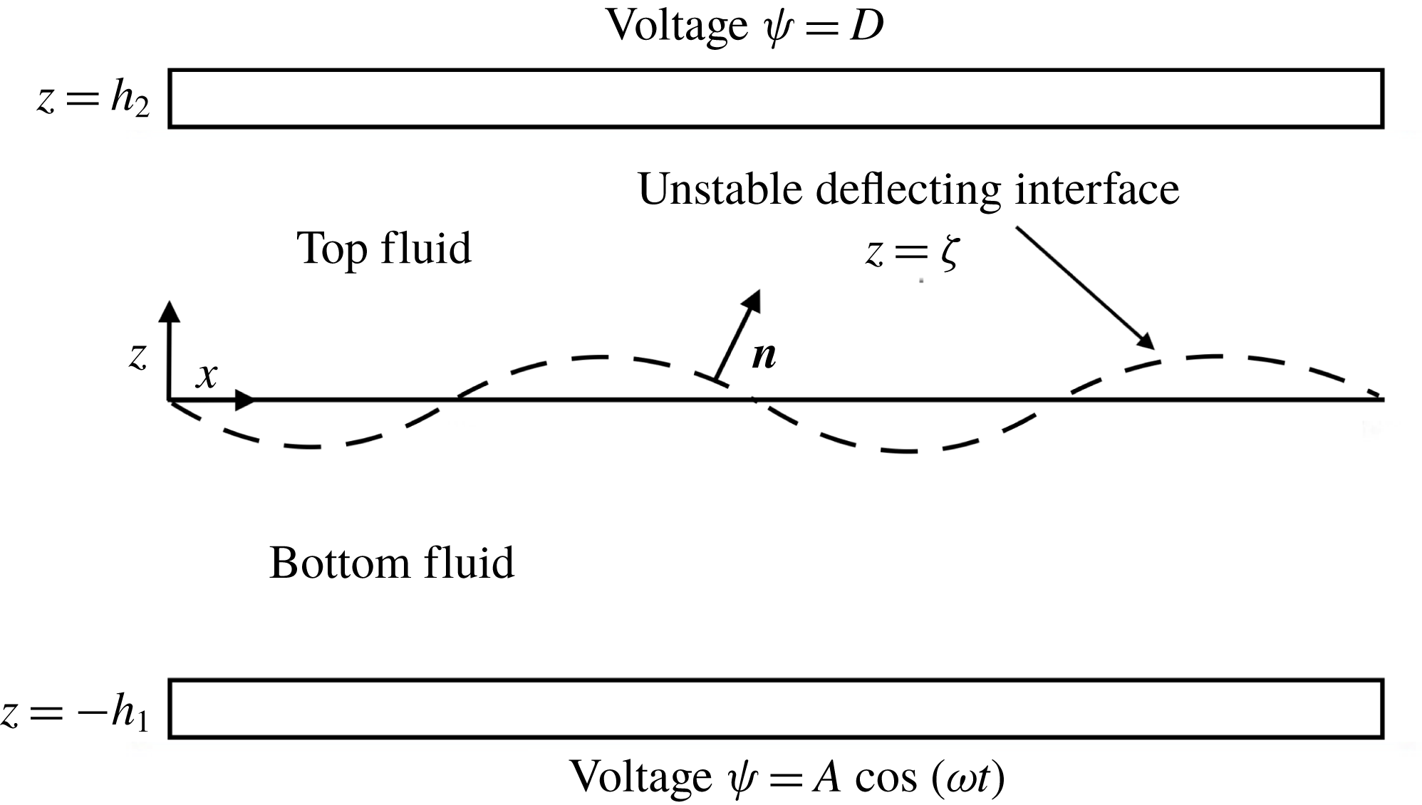
Two fluids of infinite lateral dimension are subject to an oscillatory voltage on electrodes located at the horizontal walls, located at
 $-h_{1}$
and
 $h_{2}$
, as shown in figure 1. The upper wall is held at a constant voltage
 $D$
and the lower wall at a voltage
 $A\cos (\unicode[STIX]{x1D714}t)$
. The parameter
 $D$
can take any value, including zero. Our view of the problem is this:
 $D$
and
 $\unicode[STIX]{x1D714}$
are set while
 $A$
is sequentially increased from zero until the fluid system enters a flow state, the base state being quiescent. The ultimate objective of the calculation is to plot the critical value of
 $A$
versus
 $\unicode[STIX]{x1D714}$
for the onset of flow so as to make it relevant to experiments.
Schematic of two-fluid electrostatically oscillated system. The normal vector points into the upper fluid, and the interface is taken to be initially flat and located at
 $z=0$
. The voltage on the bottom electrode is oscillated with amplitude
 $A$
and frequency
 $\unicode[STIX]{x1D714}$
, and the top electrode is held at a constant voltage
 $D$
.

Taking the index 1 to be the bottom fluid and 2 to be the top fluid, we observe that the electrostatics in the top fluid in this model are governed by Laplace’s equation for the voltage, given by
 $$\begin{eqnarray}\unicode[STIX]{x1D6FB}^{2}\unicode[STIX]{x1D713}_{2}=0,\end{eqnarray}$$
and the bottom fluid is taken to have constant potential due to its infinite conductivity. The boundary conditions for
 $\unicode[STIX]{x1D713}$
are taken as the two imposed voltages, viz.,
 $$\begin{eqnarray}\unicode[STIX]{x1D713}_{2}=D\end{eqnarray}$$
and
 $$\begin{eqnarray}\unicode[STIX]{x1D713}_{2}=A\cos \unicode[STIX]{x1D714}t\end{eqnarray}$$
at the top wall (
 $z=h_{2}$
) and at the interface (
 $z=\unicode[STIX]{x1D701}(x,t)$
), respectively.
The hydrodynamic equations in both fluids are governed by the Navier–Stokes equations along with the continuity equation, given by
 $$\begin{eqnarray}\unicode[STIX]{x1D70C}_{j}\left(\frac{\unicode[STIX]{x2202}\boldsymbol{V}_{j}}{\unicode[STIX]{x2202}t}+\boldsymbol{V}_{j}\boldsymbol{\cdot }\unicode[STIX]{x1D735}\boldsymbol{V}_{j}\right)=-\unicode[STIX]{x1D735}P_{j}+\unicode[STIX]{x1D707}_{j}\unicode[STIX]{x1D6FB}^{2}\boldsymbol{V}_{j}-\unicode[STIX]{x1D70C}_{j}g\boldsymbol{i}_{z}\end{eqnarray}$$
and
 $$\begin{eqnarray}\unicode[STIX]{x1D735}\boldsymbol{\cdot }\boldsymbol{V}_{j}=0,\end{eqnarray}$$
where
 $\boldsymbol{V}$
is the fluid velocity,
 $P$
is the pressure,
 $\unicode[STIX]{x1D707}$
is the viscosity,
 $\unicode[STIX]{x1D70C}$
is the density,
 $g$
is gravitational acceleration and
 $j=1,2$
denotes the bottom and top fluid, respectively. The hydrodynamic description is completed by no-slip and no-penetration boundary conditions on the upper and lower walls and the following interface conditions (at
 $z=\unicode[STIX]{x1D701}(x,t)$
):
 $$\begin{eqnarray}\displaystyle & \displaystyle [[\boldsymbol{V}_{j}\boldsymbol{\cdot }\boldsymbol{n}]]=0, & \displaystyle\end{eqnarray}$$
 $$\begin{eqnarray}\displaystyle & \displaystyle [[\boldsymbol{V}_{j}\boldsymbol{\cdot }\boldsymbol{t}]]=0, & \displaystyle\end{eqnarray}$$
 $$\begin{eqnarray}\displaystyle & \displaystyle [[\boldsymbol{n}\boldsymbol{\cdot }\unicode[STIX]{x1D64F}\boldsymbol{\cdot }\boldsymbol{n}]]=\unicode[STIX]{x1D6FE}2H, & \displaystyle\end{eqnarray}$$
 $$\begin{eqnarray}\displaystyle & \displaystyle [[\boldsymbol{n}\boldsymbol{\cdot }\unicode[STIX]{x1D64F}\boldsymbol{\cdot }\boldsymbol{t}]]=0, & \displaystyle\end{eqnarray}$$
along with the evolution equation for the interfacial deflection,
 $$\begin{eqnarray}[[\unicode[STIX]{x1D70C}_{j}(\boldsymbol{V}_{j}-\boldsymbol{U})\boldsymbol{\cdot }\boldsymbol{n}]]=0,\end{eqnarray}$$
where
 $\boldsymbol{n}$
is the unit normal vector pointing into the light fluid,
 $\boldsymbol{t}$
is the unit tangent vector,
 $2H$
is twice the mean surface curvature,
 $\boldsymbol{U}\boldsymbol{\cdot }\boldsymbol{n}$
is the interfacial speed and the double brackets
 $[[\unicode[STIX]{x1D719}_{j}]]$
represents
 $\unicode[STIX]{x1D719}_{2}-\unicode[STIX]{x1D719}_{1}$
.
The stress tensor
 $\unicode[STIX]{x1D64F}$
which appears in (2.8) and (2.9) is decomposed into two parts, a Maxwell stress and the hydrodynamic stress, viz.,
 $$\begin{eqnarray}\unicode[STIX]{x1D64F}=\unicode[STIX]{x1D64F}^{Maxwell}+\unicode[STIX]{x1D64F}^{Hydrodynamic},\end{eqnarray}$$
where
 $\unicode[STIX]{x1D64F}^{Hydrodynamic}$
takes its usual form and
 $\unicode[STIX]{x1D64F}^{Maxwell}$
takes the form
 $$\begin{eqnarray}\unicode[STIX]{x1D64F}^{Maxwell}=\unicode[STIX]{x1D716}\unicode[STIX]{x1D716}_{0}\boldsymbol{E}\boldsymbol{E}-{\textstyle \frac{1}{2}}\unicode[STIX]{x1D716}\unicode[STIX]{x1D716}_{0}\boldsymbol{E}\boldsymbol{\cdot }\boldsymbol{E}\unicode[STIX]{x1D644},\end{eqnarray}$$
where
 $\boldsymbol{E}=-\unicode[STIX]{x1D735}\unicode[STIX]{x1D713}$
is the electric field,
 $\unicode[STIX]{x1D716}$
is the relative permittivity of the fluid,
 $\unicode[STIX]{x1D716}_{0}$
is the permittivity of free space and
 $\unicode[STIX]{x1D644}$
is the identity tensor. Due to the simplification of the electrical properties, the normal components of the Maxwell stress can be written as
 $$\begin{eqnarray}[[\unicode[STIX]{x1D64F}^{Maxwell}\boldsymbol{\cdot }\boldsymbol{n}]]\boldsymbol{\cdot }\boldsymbol{n}={\textstyle \frac{1}{2}}[\unicode[STIX]{x1D716}_{2}\unicode[STIX]{x1D716}_{0}(-\unicode[STIX]{x1D735}\unicode[STIX]{x1D713}_{2}\boldsymbol{\cdot }\boldsymbol{n})^{2}-\unicode[STIX]{x1D716}_{2}\unicode[STIX]{x1D716}_{0}(-\unicode[STIX]{x1D735}\unicode[STIX]{x1D713}_{2}\boldsymbol{\cdot }\boldsymbol{t}_{1})^{2}-\unicode[STIX]{x1D716}_{2}\unicode[STIX]{x1D716}_{0}(-\unicode[STIX]{x1D735}\unicode[STIX]{x1D713}_{2}\boldsymbol{\cdot }\boldsymbol{t}_{2})^{2}],\end{eqnarray}$$
where
 $\boldsymbol{t}_{1}$
and
 $\boldsymbol{t}_{2}$
are unit tangent vectors. Within the perfect conductor model, there are no tangential component contributions to the Maxwell stress tensor. Thus, the velocity profiles can be solved in terms of the interface deflection,
 $\unicode[STIX]{x1D701}$
, relying on the normal stress balance, i.e. (2.8), to close the problem. This approach closely follows that of the mechanically forced problem (Kumar & Tuckerman Reference Kumar and Tuckerman1994), and the full derivation for the velocity profiles is given in appendix B.
In order to determine the stability conditions, we linearize the dependent variables about a stationary, non-deflecting interface as
 $$\begin{eqnarray}\left.\begin{array}{@{}c@{}}\unicode[STIX]{x1D713}_{2}=\unicode[STIX]{x1D713}_{2}^{0}+\unicode[STIX]{x1D713}_{2}^{\prime },\\ \unicode[STIX]{x1D701}=\unicode[STIX]{x1D701}^{\prime },\\ \boldsymbol{V}=\boldsymbol{V}^{\prime },\\ P=P^{0}+P^{\prime },\end{array}\right\}\end{eqnarray}$$
where the superscript ‘0’ represents the base state and the superscript ‘
 $^{\prime }$
’ represents the perturbed state. Inserting (2.14) into the nonlinear equations, yields (at zeroth order)
 $$\begin{eqnarray}\unicode[STIX]{x1D713}_{2}^{0}=\frac{(D-A\cos \unicode[STIX]{x1D714}t)z}{h_{2}}+A\cos \unicode[STIX]{x1D714}t\end{eqnarray}$$
and
 $$\begin{eqnarray}\frac{\text{d}P_{j}^{0}}{\text{d}z}=-\unicode[STIX]{x1D70C}_{j}g,\end{eqnarray}$$
which shows that the base state potential varies linearly through the top fluid while the base state pressure gradient is balanced by gravity.
Next, we collect the terms of order ‘
 $^{\prime }$
’ and separate variables using the traditional Floquet expansion:
 $$\begin{eqnarray}\unicode[STIX]{x1D719}^{\prime }(x,z,t)=\text{e}^{\text{i}kx}~\tilde{\unicode[STIX]{x1D719}}(z,t)=\text{e}^{\text{i}kx}\mathop{\sum }_{n=-\infty }^{\infty }\text{e}^{(\unicode[STIX]{x1D70E}+\text{i}(\unicode[STIX]{x1D6FC}+n\unicode[STIX]{x1D714}))t}\hat{\unicode[STIX]{x1D719}}_{n}(z),\end{eqnarray}$$
where
 $\unicode[STIX]{x1D719}^{\prime }$
is each of the perturbed dependent variables,
 $\unicode[STIX]{x1D70E}$
is the growth rate,
 $k$
is the wavenumber and
 $\unicode[STIX]{x1D6FC}$
can take the value of zero or
 $\unicode[STIX]{x1D714}/2$
to allow for both harmonic and subharmonic responses. We then map the dependent variables at the interface back to
 $z=0$
(Johns & Narayanan Reference Johns and Narayanan2002) to obtain the perturbed electrostatic domain equation and the accompanying boundary conditions:
 $$\begin{eqnarray}\displaystyle & \displaystyle \left(\frac{\unicode[STIX]{x2202}^{2}}{\unicode[STIX]{x2202}z^{2}}-k^{2}\right)\tilde{\unicode[STIX]{x1D713}}_{2}=0, & \displaystyle\end{eqnarray}$$
 $$\begin{eqnarray}\displaystyle & \displaystyle \tilde{\unicode[STIX]{x1D713}}_{2}|_{z=h_{2}}=0, & \displaystyle\end{eqnarray}$$
 $$\begin{eqnarray}\displaystyle & \displaystyle \left.\left(\tilde{\unicode[STIX]{x1D713}}_{2}+\tilde{\unicode[STIX]{x1D701}}\frac{\unicode[STIX]{x2202}\unicode[STIX]{x1D713}_{2}^{0}}{\unicode[STIX]{x2202}z}\right)\right|_{z=0}=0. & \displaystyle\end{eqnarray}$$
Inserting the base state voltage contributions from (2.15), expanding fully with (2.17) and solving for the perturbed voltage profile, we get (dropping hats)
 $$\begin{eqnarray}\unicode[STIX]{x1D713}_{n2}=\frac{D\unicode[STIX]{x1D701}_{n}-{\displaystyle \frac{A}{2}}(\unicode[STIX]{x1D701}_{n-1}+\unicode[STIX]{x1D701}_{n+1})}{h_{2}}(\sinh kz\coth kh_{2}-\cosh kz),\end{eqnarray}$$
which is equivalent to the Yih (Reference Yih1968) result even in the presence of viscosity due to the absence of viscosity within the electrostatic equations and the fact that the coupling between the electrostatic and hydrodynamic equations is only a one-way coupling when utilizing the perfect conductor model assumptions. Upon determination of the velocity profiles as shown in appendix B, the normal stress balance becomes
 $$\begin{eqnarray}\left[\left[\unicode[STIX]{x1D70C}_{j}(\unicode[STIX]{x1D70E}+\text{i}(\unicode[STIX]{x1D6FC}+n\unicode[STIX]{x1D714})+3\unicode[STIX]{x1D707}_{j}k^{2})\frac{\text{d}W_{nj}}{\text{d}z}-\unicode[STIX]{x1D707}_{j}\frac{\text{d}^{3}W_{nj}}{\text{d}z^{3}}\right]\right]+((\unicode[STIX]{x1D70C}_{2}-\unicode[STIX]{x1D70C}_{1})g-\unicode[STIX]{x1D6FE}k^{2})k^{2}\unicode[STIX]{x1D701}_{n}=-k^{2}\unicode[STIX]{x1D70F}^{Maxwell},\end{eqnarray}$$
where
 $W_{nj}$
is the vertical velocity component of the
 $j\text{th}$
fluid, and subscript
 $n$
is the index from (2.17). The variable,
 $\unicode[STIX]{x1D70F}^{Maxwell}$
, is defined by first taking the perturbation of (2.13) at first order, yielding the contribution of the Maxwell stress to the right-hand side of the normal stress balance, viz.,
 $$\begin{eqnarray}([[\unicode[STIX]{x1D64F}^{Maxwell}\boldsymbol{\cdot }\boldsymbol{n}]]\boldsymbol{\cdot }\boldsymbol{n})^{\prime }=\frac{\text{d}\unicode[STIX]{x1D713}_{2}^{\prime }}{\text{d}z}\frac{\unicode[STIX]{x2202}\unicode[STIX]{x1D713}_{2}^{0}}{\unicode[STIX]{x2202}z}=\unicode[STIX]{x1D702}(D^{2}-2DA\cos \unicode[STIX]{x1D714}t+A^{2}\cos ^{2}\unicode[STIX]{x1D714}t)\unicode[STIX]{x1D701}^{\prime },\end{eqnarray}$$
where
 $\unicode[STIX]{x1D702}=(k\unicode[STIX]{x1D716}_{2}\unicode[STIX]{x1D716}_{0}\coth kh_{2}/h_{2}^{2})$
. Expanding with (2.17), applying the double angle formula, and dropping hats yields
 $$\begin{eqnarray}\unicode[STIX]{x1D70F}^{Maxwell}=\unicode[STIX]{x1D702}\left(D^{2}\unicode[STIX]{x1D701}_{n}-DA(\unicode[STIX]{x1D701}_{n-1}+\unicode[STIX]{x1D701}_{n+1})+\frac{A^{2}}{4}(\unicode[STIX]{x1D701}_{n-2}+2\unicode[STIX]{x1D701}_{n}+\unicode[STIX]{x1D701}_{n+2})\right).\end{eqnarray}$$
Substitution into (2.22) and rearranging yields the final normal stress balance:
 $$\begin{eqnarray}\displaystyle & & \displaystyle \left[\left[\unicode[STIX]{x1D70C}_{j}(\unicode[STIX]{x1D70E}+\text{i}(\unicode[STIX]{x1D6FC}+n\unicode[STIX]{x1D714})+3\unicode[STIX]{x1D707}_{j}k^{2})\frac{\text{d}W_{nj}}{\text{d}z}-\unicode[STIX]{x1D707}_{j}\frac{\text{d}^{3}W_{nj}}{\text{d}z^{3}}\right]\right]+((\unicode[STIX]{x1D70C}_{2}-\unicode[STIX]{x1D70C}_{1})g+\unicode[STIX]{x1D702}D^{2}-\unicode[STIX]{x1D6FE}k^{2})k^{2}\unicode[STIX]{x1D701}_{n}\nonumber\\ \displaystyle & & \displaystyle \qquad =Ak^{2}\unicode[STIX]{x1D702}D(\unicode[STIX]{x1D701}_{n-1}+\unicode[STIX]{x1D701}_{n+1})-A^{2}\frac{k^{2}\unicode[STIX]{x1D702}}{4}(\unicode[STIX]{x1D701}_{n-2}+2\unicode[STIX]{x1D701}_{n}+\unicode[STIX]{x1D701}_{n+2}).\end{eqnarray}$$
This expression is similar to that obtained for the mechanically forced Faraday instability (Kumar & Tuckerman Reference Kumar and Tuckerman1994), with additional constant voltage terms and a modified time dependent forcing, here with both harmonic and twice harmonic components, arising from
 $\cos ^{2}(\unicode[STIX]{x1D714}t)$
. To consider neutral stability, we set
 $\unicode[STIX]{x1D70E}$
to zero and then cast (2.25) as a polynomial eigenvalue problem with the form
 $$\begin{eqnarray}B_{n}\unicode[STIX]{x1D701}_{n}=CA\unicode[STIX]{x1D701}_{n}+EA^{2}\unicode[STIX]{x1D701}_{n},\end{eqnarray}$$
where
 $B_{n}$
is a coefficient of the
 $A$
independent terms and where
 $C$
and
 $E$
are the coefficients of
 $A$
and
 $A^{2}$
terms, respectively. It is first important to note that within (2.26) we seek the critical values of
 $A$
, i.e. the amplitude of the imposed oscillatory voltage. It is also important to note that both
 $C$
and
 $E$
are purely real. The reality conditions inherent to (2.17) are the same as those found in mechanical Faraday instability calculations for the
 $\unicode[STIX]{x1D701}_{-1}$
terms, i.e.
 $\unicode[STIX]{x1D701}_{-1}=\bar{\unicode[STIX]{x1D701}_{1}}$
for
 $\unicode[STIX]{x1D6FC}=0$
and
 $\unicode[STIX]{x1D701}_{-1}=\bar{\unicode[STIX]{x1D701}_{0}}$
for
 $\unicode[STIX]{x1D6FC}=(\unicode[STIX]{x1D714}/2)$
along with the conditions for the
 $\unicode[STIX]{x1D701}_{-2}$
terms
 $\unicode[STIX]{x1D701}_{-2}=\bar{\unicode[STIX]{x1D701}_{2}}$
for
 $\unicode[STIX]{x1D6FC}=0$
and
 $\unicode[STIX]{x1D701}_{-2}=\bar{\unicode[STIX]{x1D701}_{1}}$
for
 $\unicode[STIX]{x1D6FC}=(\unicode[STIX]{x1D714}/2)$
. Here, the overbar indicates complex conjugates. To enforce the reality conditions, equation (2.26) can be separated into its real and complex parts, producing the final matrix equation governing the system stability:
 $$\begin{eqnarray}\bar{\unicode[STIX]{x1D63D}}\bar{\unicode[STIX]{x1D701}}=A\bar{\unicode[STIX]{x1D63E}}\bar{\unicode[STIX]{x1D701}}+A^{2}\bar{\unicode[STIX]{x1D640}}\bar{\unicode[STIX]{x1D701}},\end{eqnarray}$$
where the matrices
 $\bar{\unicode[STIX]{x1D63D}}$
,
 $\bar{\unicode[STIX]{x1D63E}}$
and
 $\bar{\unicode[STIX]{x1D640}}$
are shown in appendix C.
For the current study, the index
 $n$
was typically truncated at a value of 12. Including higher
 $n$
values within the calculation added computational time and did not significantly alter the results. This polynomial eigenvalue problem is then solved using the ‘polyeig’ command within Matlab®, where the lowest, positive eigenvalue calculated is the critical amplitude,
 $A$
, for the input frequency,
 $\unicode[STIX]{x1D714}$
, wavenumber,
 $k$
and
 $\unicode[STIX]{x1D6FC}$
value of either
 $\unicode[STIX]{x1D6FC}=0$
or
 $\unicode[STIX]{x1D6FC}=(\unicode[STIX]{x1D714}/2)$
. Such a calculation yields the lowest of the critical amplitudes,
 $A$
, the corresponding wavenumber,
 $k$
, and the harmonic nature of the response.
2.2 Calculations for the perfect conductor model
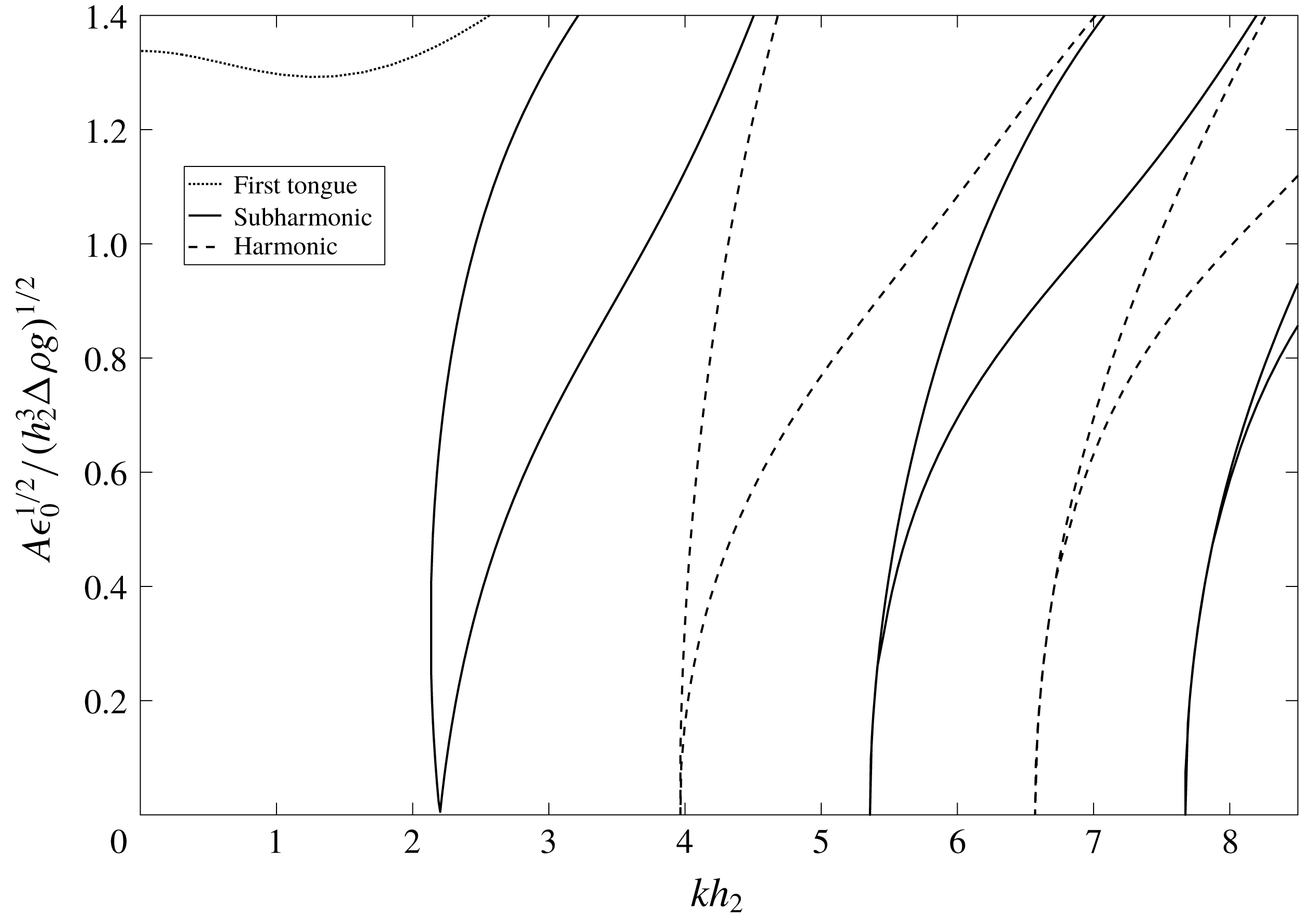
The inviscid electrostatically forced Faraday instability produces a Mathieu equation as shown by Yih (Reference Yih1968) and re-derived for the reader’s convenience in appendix A. Figure 2 shows the results from the eigenvalue problem arising from the Mathieu equation cast into the familiar
 $A$
versus
 $k$
form for comparison to the upcoming viscous results. The figures are given in scaled form, where the voltage scale arises from (2.25) and the wavenumber is scaled by the height of the insulating fluid. The calculations are performed assuming the properties of water and air. Alternating subharmonic and harmonic tongues similar to those seen in mechanically forced Faraday instability problems (Benjamin & Ursell Reference Benjamin and Ursell1954) are found for
 $D\neq 0$
, and the minimum threshold amplitude of each tongue is zero at the resonance points.
Scaled amplitude versus wavenumber for
 $D=5000$
V calculated from the inviscid perfect conductor model. Alternating subharmonic and harmonic tongues are obtained when
 $D\neq 0$
. Fluid parameters are
 $\unicode[STIX]{x1D70C}_{1}=1000~\text{kg}~\text{m}^{-3}$
,
 $\unicode[STIX]{x1D70C}_{2}=1.225~\text{kg}~\text{m}^{-3}$
,
 $h_{1}=h_{2}=6$
mm,
 $\unicode[STIX]{x1D716}_{2}=1.00059$
,
 $\unicode[STIX]{x1D6FE}=0.07275~\text{kg}~\text{s}^{-2}$
and
 $\unicode[STIX]{x1D714}=25$
Hz.

The addition of viscosity into the problem also results in alternating subharmonic and harmonic tongues when
 $D\neq 0$
. Predictably, the minimum threshold of each tongue is finite, and increases with increasing wavenumber due to increased viscous damping from the choppier modes. In the case of
 $D=0$
, for both viscous and inviscid fluids only harmonic tongues can be obtained. This is due to the fact that the voltage enters into the normal stress balance only as a squared term, i.e.
 $\cos ^{2}(\unicode[STIX]{x1D714}t)$
. When
 $D=0$
is imposed, the
 $\cos (\unicode[STIX]{x1D714}t)$
terms vanish from (2.23), leaving only
 $\cos ^{2}(\unicode[STIX]{x1D714}t)$
terms coming from the electrostatic forcing. The squared nature of these terms gives rise to a periodic forcing that is twice harmonic with the imposed frequency. In this case, the lowest possible response frequency is half of this forcing, therefore harmonic with the imposed frequency. However if
 $D\neq 0$
is set, the forcing consists of
 $\cos (\unicode[STIX]{x1D714}t)$
and
 $\cos ^{2}(\unicode[STIX]{x1D714}t)$
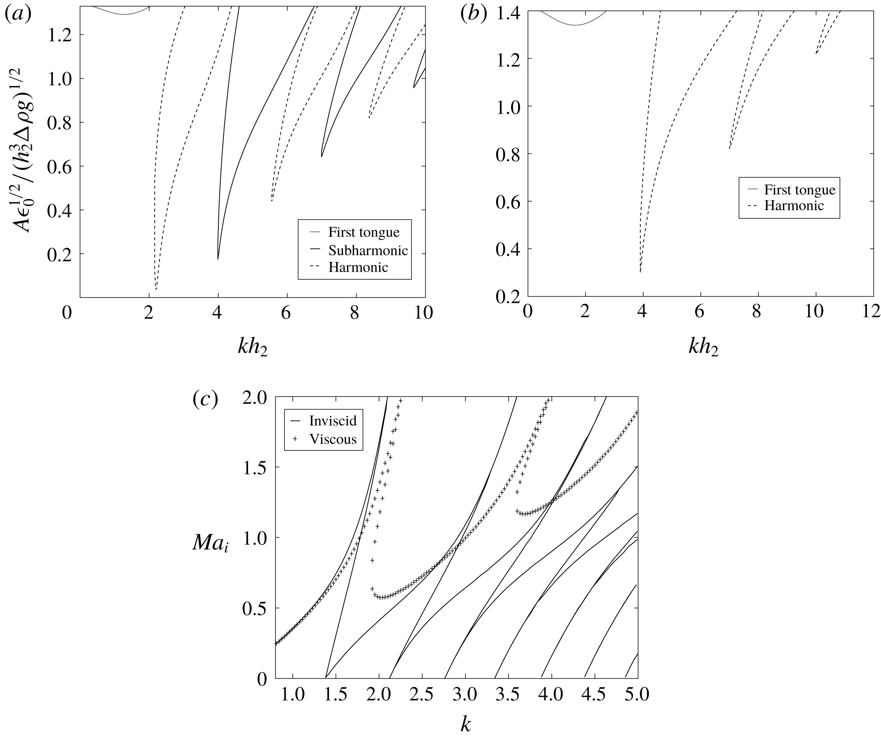
terms. This allows the response to contain a subharmonic component as well as a harmonic component. Figure 3(a,b) shows the stability tongues for both cases, i.e.
 $D\neq 0$
and
 $D=0$
, now for the case of viscous fluids. In addition, figure 3(c) shows that the model is able to recover the Bandopadhyay & Hardt (Reference Bandopadhyay and Hardt2017) results in both the inviscid and viscous cases after rescaling.
Scaled
 $A$
versus
 $k$
for both (a)
 $D=5000$
V and (b)
 $D=0$
. Fluid parameters are
 $\unicode[STIX]{x1D707}_{1}=0.001~\text{kg}~\text{ms}^{-1}$
,
 $\unicode[STIX]{x1D707}_{2}=1.983\times 10^{-5}~\text{kg}~\text{ms}^{-1}$
and other parameters equivalent to those in figure 2. Alternating subharmonic and harmonic tongues are seen when
 $D\neq 0$
, while only harmonic tongues are observable when
 $D=0$
. (c) Reproduction of figure 3(a) of Bandopadhyay & Hardt (Reference Bandopadhyay and Hardt2017). The current model is able to recover the previously reported results in addition to the first tongue, not reported earlier. Fluid parameters and
 $Ma_{i}$
are those given and defined by Bandopadhyay & Hardt (Reference Bandopadhyay and Hardt2017).

Another peculiar characteristic of the electrostatic forcing comes in the form of an additional tongue, labelled in figure 3 as ‘first tongue’, which does not behave in the same manner as the others. This tongue is harmonic in nature, and specifically arises from the non-periodic stress terms that can be seen in (2.27). This tongue is not reported by Bandopadhyay & Hardt (Reference Bandopadhyay and Hardt2017), though this region may prove to be important in certain circumstances where low wavenumbers can be accessed. These terms have two origins: one from the constant voltage on the top plate (
 $D$
) and one from the non-periodic term generated through the use of the double angle formula. In the absence of periodic forcing, i.e. when
 $\unicode[STIX]{x1D714}=0$
, the ‘first tongue’ is in fact the only stability tongue, and is generated as a balance between the constant voltage stress term and
 $(\unicode[STIX]{x1D70C}_{2}-\unicode[STIX]{x1D70C}_{1})g-\unicode[STIX]{x1D6FE}k^{2}$
. This balance is given by
 $$\begin{eqnarray}(\unicode[STIX]{x1D70C}_{2}-\unicode[STIX]{x1D70C}_{1})g-\unicode[STIX]{x1D6FE}k^{2}=-D^{2}\unicode[STIX]{x1D702}\end{eqnarray}$$
for the perfect conductor model, where the value of
 $D$
that satisfies this equation for a given
 $k$
value is the critical value of
 $D$
which is found on the first tongue. Equation (2.28) can be seen from the equation for the natural frequency in the Yih model (see appendix A) when the natural frequency is set equal to zero and is understandably independent of viscosity. The balance is similar in nature, albeit more complicated, for the leaky dielectric case. This tongue depicts the point where the time-independent components of the electrostatic stresses just commence to overwhelm the stabilizing effect of gravity and interfacial tension, allowing for destabilization of the interface.
The tongue still appears even in the absence of a constant voltage on the top plate when imposing a periodic forcing. The balance that leads to the critical amplitude, however, is not given by merely adding the term generated from the double angle formula to (2.28), as
 $$\begin{eqnarray}(\unicode[STIX]{x1D70C}_{2}-\unicode[STIX]{x1D70C}_{1})g-\unicode[STIX]{x1D6FE}k^{2}=-D^{2}\unicode[STIX]{x1D702}-\frac{A^{2}\unicode[STIX]{x1D702}}{2}.\end{eqnarray}$$
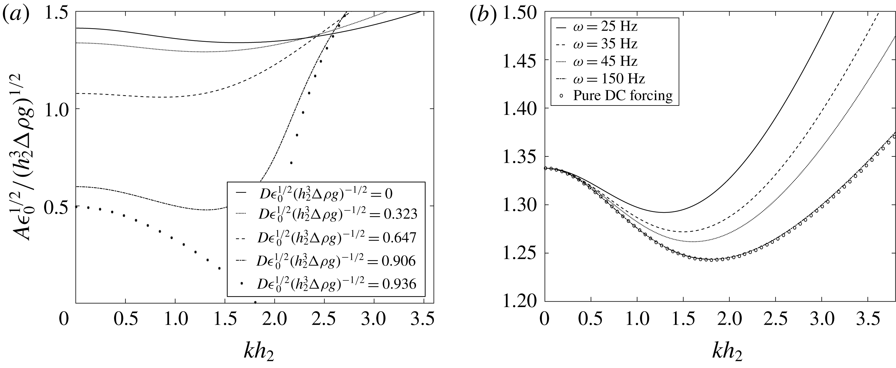
Instead, the physics arising from the oscillatory forcing alters the tongue’s behaviour, such that it asymptotes with the first subharmonic tongue solution with increasing wavenumber. The eigenvalues of the tongue do correspond to those given by solving (2.29) for low wavenumbers, with the wavenumber range in which the two results correspond expanding with increasing frequency. This compares favourably with the accepted thought that applying a high frequency voltage oscillation produces almost identical behaviour to imposing a constant voltage drop. Since this tongue is always present, an inherent feature of the problem is a threshold amplitude below the first Faraday tongue for low wavenumbers. Contrast this to the mechanical Faraday problem (Kumar & Tuckerman Reference Kumar and Tuckerman1994), where at very low wavenumbers the critical amplitude becomes extremely high. In the case of electrostatic forcing, at very low wavenumbers the critical amplitude is bounded by the first tongue.
Since the effects of the constant voltage offset and the constant terms arising from the periodic forcing are additive, it is easily seen that
 $A_{\ast }$
, defined as the critical amplitude for the first tongue, decreases with increasing
 $D$
. Figure 4 shows this effect for multiple values of
 $D$
. The tongue will continue to shift to lower critical amplitudes until
 $(\unicode[STIX]{x1D70C}_{2}-\unicode[STIX]{x1D70C}_{1})g-\unicode[STIX]{x1D6FE}k^{2}+D^{2}\unicode[STIX]{x1D702}=0$
. For the fluid parameters tested (see figure captions), this phenomenon first occurs at
 $D=14.47826$
kV. At this point, the system is unstable to one wavelength with any finite amplitude of oscillation. However, shorter wavelengths are able to be stabilized due to the hidden
 $k$
inside the
 $\unicode[STIX]{x1D702}$
parameter (see (2.23)).
(a) Effect of
 $D$
on the first harmonic tongue. The tongue shifts down in critical amplitude with increasing
 $D$
, and first reaches a critical amplitude of 0 for
 $D\approx 14.48$
kV at
 $k=301~\text{m}^{-1}$
for the fluid parameters given in figure 3(a,b). (b) Effect of frequency on the first harmonic tongue. As frequency increases, the tongue approaches the pure DC electrostatic Rayleigh–Taylor instability solution.
 $D$
is held at 5 kV for all tested frequencies.

Figure 5 shows the effect of changing
 $D$
on the instability thresholds. It can clearly be seen that for subharmonic tongues, an increase in
 $D$
causes the tongues to shift to higher wavenumber and lower critical amplitude. We also observe a narrowing of the tongues with decreasing wavenumber. This trend continues as
 $D$
decreases, eventually leading to extremely high threshold amplitudes as
 $D$
approaches zero. Harmonic tongues also shift to higher wavenumber and lower critical amplitude with increasing
 $D$
. However, this effect is much less pronounced than the subharmonic tongues. In addition, narrowing of the harmonic tongues occur to a much lesser extent with decreasing
 $D$
. The increased effect of
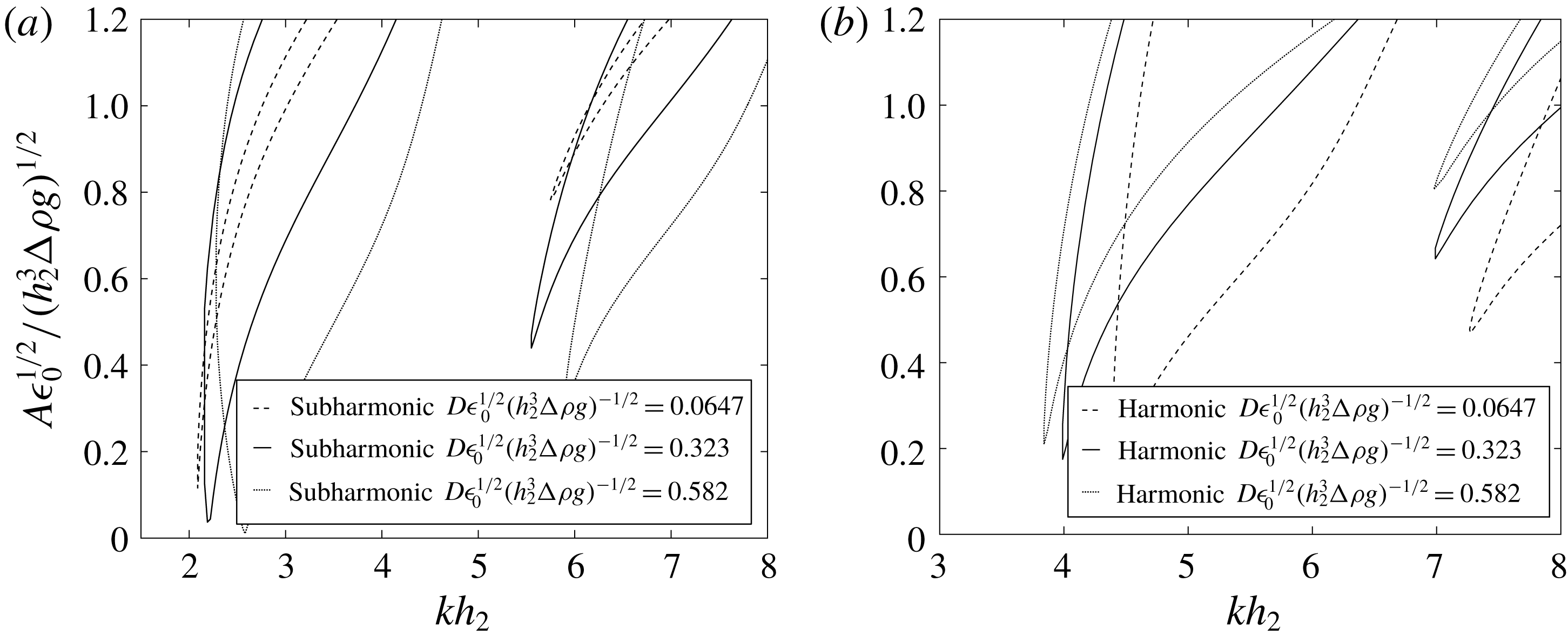
 $D$
on the subharmonic stability tongues again lends itself to the fact that subharmonic tongues are only achievable with finite
 $D$
values, while harmonic tongues are achievable with
 $D=0$
.
Effect of varying
 $D$
on stability thresholds for both subharmonic (a) and harmonic (b) responses. Fluid properties are the same as those shown in figure 3(a). Increasing
 $D$
has the general effect of widening the instability tongues and causing a shift to higher wavenumber and lower threshold amplitude. The first harmonic tongues discussed previously are omitted for clarity.

2.3 Leaky dielectric model
The leaky dielectric model (LD) is also analysed through linear stability with the hydrodynamics aspect again following closely to the Kumar & Tuckerman (Reference Kumar and Tuckerman1994) model, modified by terms arising from the Maxwell stress (Saville Reference Saville1997). This model is adapted by simultaneously solving the electrostatic equations to determine the Maxwell stress contributions, which are more complicated than those obtained in the perfect conductor model. Since the assumptions on the fluid electrical properties are relaxed, we can no longer decouple the perturbed voltage profiles with the perturbed hydrodynamic equations. Again, figure 1 shows the problem schematic, which is considered as a horizontally infinite two-fluid system.
Both fluids are now taken to be viscous, leaky dielectrics with no charged species present inside the fluid bodies, with both fluids exhibiting isotropic dielectric constants. Since the body force terms arising from the Maxwell stress are absent, the hydrodynamics in both fluids are again governed by the Navier–Stokes equations coupled with the continuity equation, given by (2.4)–(2.10), where the electrostatic forcing again enters into the problem only through the stress tensor at the interface (see (2.11)). In the LD model, the normal component of the Maxwell stress is given by
 $$\begin{eqnarray}[[\unicode[STIX]{x1D64F}^{Maxwell}\boldsymbol{\cdot }\boldsymbol{n}]]\boldsymbol{\cdot }\boldsymbol{n}={\textstyle \frac{1}{2}}[[\unicode[STIX]{x1D716}_{j}\unicode[STIX]{x1D716}_{0}(-\unicode[STIX]{x1D735}\unicode[STIX]{x1D713}_{j}\boldsymbol{\cdot }\boldsymbol{n})^{2}-\unicode[STIX]{x1D716}_{j}\unicode[STIX]{x1D716}_{0}(-\unicode[STIX]{x1D735}\unicode[STIX]{x1D713}_{j}\boldsymbol{\cdot }\boldsymbol{t}_{1})^{2}-\unicode[STIX]{x1D716}_{j}\unicode[STIX]{x1D716}_{0}(-\unicode[STIX]{x1D735}\unicode[STIX]{x1D713}_{j}\boldsymbol{\cdot }\boldsymbol{t}_{2})^{2}]]\end{eqnarray}$$
and the leaky dielectric nature of the fluids now also allows tangential components of the Maxwell stress, viz.,
 $$\begin{eqnarray}[[\unicode[STIX]{x1D64F}^{Maxwell}\boldsymbol{\cdot }\boldsymbol{n}]]\boldsymbol{\cdot }\boldsymbol{t}=-q\unicode[STIX]{x1D735}\unicode[STIX]{x1D713}\boldsymbol{\cdot }\boldsymbol{t},\end{eqnarray}$$
where
 $q$
is the interfacial charge density.
The electrostatics in both fluids are now governed by Laplace’s equation:
 $$\begin{eqnarray}\unicode[STIX]{x1D6FB}^{2}\unicode[STIX]{x1D713}_{j}=0\end{eqnarray}$$
with the boundary conditions
 $$\begin{eqnarray}\unicode[STIX]{x1D713}_{2}=D\end{eqnarray}$$
and
 $$\begin{eqnarray}\unicode[STIX]{x1D713}_{1}=A\cos \unicode[STIX]{x1D714}t\end{eqnarray}$$
at the top (
 $z=h_{2}$
) and bottom (
 $z=-h_{1}$
) walls, respectively. The interfacial conditions are given by
 $$\begin{eqnarray}\unicode[STIX]{x1D713}_{2}=\unicode[STIX]{x1D713}_{1}\end{eqnarray}$$
and
 $$\begin{eqnarray}q(x,y,t)=[[-\unicode[STIX]{x1D716}_{j}\unicode[STIX]{x1D716}_{0}\unicode[STIX]{x1D735}\unicode[STIX]{x1D713}_{j}]]\boldsymbol{\cdot }\boldsymbol{n}\end{eqnarray}$$
and the problem specification is completed by the interfacial charge equation
 $$\begin{eqnarray}\frac{\unicode[STIX]{x2202}q}{\unicode[STIX]{x2202}t}=q\boldsymbol{n}\boldsymbol{\cdot }(\boldsymbol{n}\boldsymbol{\cdot }\unicode[STIX]{x1D735})\boldsymbol{V}+q(\boldsymbol{U}\boldsymbol{\cdot }\boldsymbol{n})2H-V_{x}\cdot \frac{\unicode[STIX]{x2202}q}{\unicode[STIX]{x2202}x}+[[\unicode[STIX]{x1D70E}_{j}\unicode[STIX]{x1D735}\unicode[STIX]{x1D713}_{j}\boldsymbol{\cdot }\boldsymbol{n}]]\quad \text{at }z=\unicode[STIX]{x1D701}(x,t),\end{eqnarray}$$
where
 $V_{x}$
is the
 $x$
-component of the velocity and
 $\unicode[STIX]{x1D70E}_{j}$
is the electrical conductivity of fluid
 $j$
.
The dependent variables are once again linearized about a quiescent, non-deflecting interface in the same manner as previously shown. Upon collection of the base state terms, the electrostatics domain equations become
 $$\begin{eqnarray}\frac{\unicode[STIX]{x2202}^{2}\unicode[STIX]{x1D713}_{j}^{0}}{\unicode[STIX]{x2202}z^{2}}=0.\end{eqnarray}$$
The base state boundary conditions are given by
 $$\begin{eqnarray}\left.\begin{array}{@{}c@{}}\displaystyle \unicode[STIX]{x1D713}_{2}^{0}=D\quad \text{at }z=h_{2},\\ \displaystyle \unicode[STIX]{x1D713}_{1}^{0}=A\cos \unicode[STIX]{x1D714}t\quad \text{at }z=-h_{1},\\ \displaystyle \unicode[STIX]{x1D713}_{2}^{0}=\unicode[STIX]{x1D713}_{1}^{0}\quad \text{at }z=0,\\ \displaystyle q^{0}=\left[\left[-\unicode[STIX]{x1D716}_{0}\unicode[STIX]{x1D716}_{j}\frac{\unicode[STIX]{x2202}\unicode[STIX]{x1D713}_{j}}{\unicode[STIX]{x2202}z}\right]\right]\quad \text{at }z=0,\end{array}\right\}\end{eqnarray}$$
and the base state charge evolution equation is
 $$\begin{eqnarray}\frac{\unicode[STIX]{x2202}q^{0}}{\unicode[STIX]{x2202}t}=\left[\left[\unicode[STIX]{x1D70E}_{j}\frac{\unicode[STIX]{x2202}\unicode[STIX]{x1D713}_{j}^{0}}{\unicode[STIX]{x2202}z}\right]\right]\end{eqnarray}$$
since the base state is quiescent. The base state is solved by first obtaining the voltage profiles in terms of
 $q$
for both fluids, resulting in
 $$\begin{eqnarray}\left.\begin{array}{@{}c@{}}\displaystyle \unicode[STIX]{x1D713}_{1}^{0}=\frac{h_{2}(q^{0}z+q^{0}h_{1}+\unicode[STIX]{x1D716}_{0}\unicode[STIX]{x1D716}_{1}A\cos \unicode[STIX]{x1D714}t)+\unicode[STIX]{x1D716}_{0}\unicode[STIX]{x1D716}_{2}((D-A\cos \unicode[STIX]{x1D714}t)z+Dh_{1})}{\unicode[STIX]{x1D716}_{0}(h_{2}\unicode[STIX]{x1D716}_{1}+h_{1}\unicode[STIX]{x1D716}_{2})},\\ \displaystyle \unicode[STIX]{x1D713}_{2}^{0}=\frac{h_{1}(-q^{0}z+q^{0}h_{2}+D\unicode[STIX]{x1D716}_{0}\unicode[STIX]{x1D716}_{2})+\unicode[STIX]{x1D716}_{0}\unicode[STIX]{x1D716}_{1}(h_{2}A\cos \unicode[STIX]{x1D714}t+z(D-A\cos \unicode[STIX]{x1D714}t))}{\unicode[STIX]{x1D716}_{0}(h_{2}\unicode[STIX]{x1D716}_{1}+h_{1}\unicode[STIX]{x1D716}_{2})}.\end{array}\right\}\end{eqnarray}$$
We then assume that the base state charge density takes the form
 $$\begin{eqnarray}q^{0}=\hat{q}+\tilde{\tilde{q}}\text{e}^{\text{i}\unicode[STIX]{x1D714}t}+\bar{q}\text{e}^{-\text{i}\unicode[STIX]{x1D714}t}\end{eqnarray}$$
due to the periodic nature of the voltage profiles. Upon substitution of (2.41) and (2.42) into (2.40), evaluation of the derivatives, and combining like terms, the expression for
 $q^{0}$
is obtained by
 $$\begin{eqnarray}\left.\begin{array}{@{}c@{}}\displaystyle \hat{q}=\frac{-D\unicode[STIX]{x1D716}_{0}(\unicode[STIX]{x1D716}_{2}\unicode[STIX]{x1D70E}_{1}-\unicode[STIX]{x1D716}_{1}\unicode[STIX]{x1D70E}_{2})}{h_{2}\unicode[STIX]{x1D70E}_{1}+h_{1}\unicode[STIX]{x1D70E}_{2}}=F_{1},\\ \displaystyle \tilde{\tilde{q}}=\frac{\text{i}A\unicode[STIX]{x1D716}_{0}(\unicode[STIX]{x1D716}_{2}\unicode[STIX]{x1D70E}_{1}-\unicode[STIX]{x1D716}_{1}\unicode[STIX]{x1D70E}_{2})}{2(h_{2}(\unicode[STIX]{x1D714}\unicode[STIX]{x1D716}_{0}\unicode[STIX]{x1D716}_{1}+\text{i}\unicode[STIX]{x1D70E}_{1})+h_{1}(\unicode[STIX]{x1D714}\unicode[STIX]{x1D716}_{0}\unicode[STIX]{x1D716}_{2}+\text{i}\unicode[STIX]{x1D70E}_{2}))}=A~F_{2}\end{array}\right\}\end{eqnarray}$$
and
 $$\begin{eqnarray}\bar{q}=\frac{-\text{i}A\unicode[STIX]{x1D716}_{0}(\unicode[STIX]{x1D716}_{2}\unicode[STIX]{x1D70E}_{1}-\unicode[STIX]{x1D716}_{1}\unicode[STIX]{x1D70E}_{2})}{2(h_{2}(\unicode[STIX]{x1D714}\unicode[STIX]{x1D716}_{0}\unicode[STIX]{x1D716}_{1}-\text{i}\unicode[STIX]{x1D70E}_{1})+h_{1}(\unicode[STIX]{x1D714}\unicode[STIX]{x1D716}_{0}\unicode[STIX]{x1D716}_{2}-\text{i}\unicode[STIX]{x1D70E}_{2}))}=A~\bar{F}_{2},\end{eqnarray}$$
where
 $F_{1}$
and
 $F_{2}$
are constants only dependent on input parameters. It is easily seen that
 $q^{0}$
and therefore
 $\unicode[STIX]{x1D713}_{1}^{0}$
and
 $\unicode[STIX]{x1D713}_{2}^{0}$
are independent of
 $x$
and vary periodically with the imposed forcing. It should be noted here that in the limit of
 $\unicode[STIX]{x1D70E}_{1}\rightarrow \infty$
, the base state voltage profiles approach those observed using the perfect conductor model.
The base state electrostatics are now completely known and thus the next step is to collect terms of order ‘
 $^{\prime }$
’, using (2.17) to obtain the perturbed domain equation
 $$\begin{eqnarray}\left(\frac{\unicode[STIX]{x2202}^{2}}{\unicode[STIX]{x2202}z^{2}}-k^{2}\right)\tilde{\unicode[STIX]{x1D713}}_{j}=0\end{eqnarray}$$
and its corresponding boundary conditions
 $$\begin{eqnarray}\left.\begin{array}{@{}c@{}}\displaystyle \tilde{\unicode[STIX]{x1D713}}_{1}=0\quad \text{at }z=-h_{1},\\ \displaystyle \tilde{\unicode[STIX]{x1D713}}_{2}=0\quad \text{at }z=h_{2},\\ \displaystyle \tilde{\unicode[STIX]{x1D713}}_{1}+\tilde{\unicode[STIX]{x1D701}}\frac{\unicode[STIX]{x2202}\unicode[STIX]{x1D713}_{1}^{0}}{\unicode[STIX]{x2202}z}=\tilde{\unicode[STIX]{x1D713}}_{2}+\tilde{\unicode[STIX]{x1D701}}\frac{\unicode[STIX]{x2202}\unicode[STIX]{x1D713}_{2}^{0}}{\unicode[STIX]{x2202}z}\quad \text{at }z=0\\ \end{array}\right\}\end{eqnarray}$$
and
 $$\begin{eqnarray}\tilde{q}=\left[\left[-\unicode[STIX]{x1D716}_{0}\unicode[STIX]{x1D716}_{j}\frac{\unicode[STIX]{x2202}\tilde{\unicode[STIX]{x1D713}}_{j}}{\unicode[STIX]{x2202}z}\right]\right]\quad \text{at }z=0\end{eqnarray}$$
along with the perturbed interfacial charge equation
 $$\begin{eqnarray}\frac{\unicode[STIX]{x2202}\tilde{q}}{\unicode[STIX]{x2202}t}=q^{0}\frac{\unicode[STIX]{x2202}\tilde{W}_{1}}{\unicode[STIX]{x2202}z}+\left[\left[\unicode[STIX]{x1D70E}_{j}\frac{\unicode[STIX]{x2202}\tilde{\unicode[STIX]{x1D713}}_{j}}{\unicode[STIX]{x2202}z}\right]\right]\!,\end{eqnarray}$$
where
 $W$
is the
 $z$
-component of the perturbed velocity.
The perturbed hydrodynamic equations follow the equations given in appendix B with changes only occurring in the tangential and normal components of the stress balance. The perturbed tangential stress balance becomes
 $$\begin{eqnarray}\unicode[STIX]{x1D707}_{2}\left(\frac{\unicode[STIX]{x2202}^{2}}{\unicode[STIX]{x2202}z^{2}}+k^{2}\right)\tilde{W}_{2}-\unicode[STIX]{x1D707}_{1}\left(\frac{\unicode[STIX]{x2202}^{2}}{\unicode[STIX]{x2202}z^{2}}+k^{2}\right)\tilde{W}_{1}=q^{0}k^{2}\left(\tilde{\unicode[STIX]{x1D713}_{1}}+\tilde{\unicode[STIX]{x1D701}}\frac{\unicode[STIX]{x2202}\unicode[STIX]{x1D713}_{1}^{0}}{\unicode[STIX]{x2202}z}\right)\end{eqnarray}$$
and the perturbed normal stress balance becomes
 $$\begin{eqnarray}\displaystyle & & \displaystyle \left[\left[\unicode[STIX]{x1D70C}_{j}\left(\frac{\unicode[STIX]{x2202}}{\unicode[STIX]{x2202}t}+3\unicode[STIX]{x1D707}_{j}k^{2}\right)\frac{\unicode[STIX]{x2202}\tilde{W}_{j}}{\text{d}z}-\unicode[STIX]{x1D707}_{j}\frac{\unicode[STIX]{x2202}^{3}\tilde{W}_{j}}{\text{d}z^{3}}\right]\right]+((\unicode[STIX]{x1D70C}_{2}-\unicode[STIX]{x1D70C}_{1})g-\unicode[STIX]{x1D6FE}k^{2})k^{2}\tilde{\unicode[STIX]{x1D701}}\nonumber\\ \displaystyle & & \displaystyle \qquad =-k^{2}\unicode[STIX]{x1D716}_{0}\left(\unicode[STIX]{x1D716}_{2}\left(\frac{\unicode[STIX]{x2202}\tilde{\unicode[STIX]{x1D713}}_{2}}{\text{d}z}\frac{\unicode[STIX]{x2202}\unicode[STIX]{x1D713}_{2}^{0}}{\unicode[STIX]{x2202}z}\right)-\unicode[STIX]{x1D716}_{1}\left(\frac{\unicode[STIX]{x2202}\tilde{\unicode[STIX]{x1D713}}_{1}}{\unicode[STIX]{x2202}z}\frac{\unicode[STIX]{x2202}\unicode[STIX]{x1D713}_{1}^{0}}{\unicode[STIX]{x2202}z}\right)\right).\end{eqnarray}$$
The perturbed velocity and voltage profiles must be solved simultaneously due to their coupling, and thus the remainder of the derivation is performed symbolically. Equation (2.48) is used to eliminate
 $\tilde{q}$
from the perturbed voltage boundary conditions, and the resultant set of boundary condition equations for both voltage and velocity are fully expanded using (2.17) and solved symbolically and computationally using Mathematica®. The analysis follows identically to that given in § 2.1. Once obtained, the profiles are substituted into (2.50), combining terms with common orders of
 $A$
. This results in two distinct cases: for
 $D=0$
,
 $$\begin{eqnarray}\displaystyle U_{1}\unicode[STIX]{x1D701}_{n} & = & \displaystyle A^{2}(Y_{2}\unicode[STIX]{x1D701}_{n}+Y_{3}\unicode[STIX]{x1D701}_{n-2}+Y_{4}\unicode[STIX]{x1D701}_{n+2})+A^{4}(Y_{5}\unicode[STIX]{x1D701}_{n}+Y_{6}\unicode[STIX]{x1D701}_{n-2}+Y_{7}\unicode[STIX]{x1D701}_{n+2}+Y_{8}\unicode[STIX]{x1D701}_{n-4}+Y_{9}\unicode[STIX]{x1D701}_{n+4})\nonumber\\ \displaystyle & & \displaystyle +\,A^{6}(Y_{10}\unicode[STIX]{x1D701}_{n}+Y_{11}\unicode[STIX]{x1D701}_{n-2}+Y_{12}\unicode[STIX]{x1D701}_{n+2}+Y_{13}\unicode[STIX]{x1D701}_{n-4}+Y_{14}\unicode[STIX]{x1D701}_{n+4}+Y_{15}\unicode[STIX]{x1D701}_{n-6}+Y_{16}\unicode[STIX]{x1D701}_{n+6}),\nonumber\\ \displaystyle & & \displaystyle\end{eqnarray}$$
and for
 $D\neq 0$
,
 $$\begin{eqnarray}\displaystyle Y_{1}\unicode[STIX]{x1D701}_{n} & = & \displaystyle A(Z_{2}\unicode[STIX]{x1D701}_{n-1}+Z_{3}\unicode[STIX]{x1D701}_{n+1})+A^{2}(Z_{4}\unicode[STIX]{x1D701}_{n}+Z_{5}\unicode[STIX]{x1D701}_{n-2}+Z_{6}\unicode[STIX]{x1D701}_{n+2})\nonumber\\ \displaystyle & & \displaystyle +\,A^{3}(Z_{7}\unicode[STIX]{x1D701}_{n-1}+Z_{8}\unicode[STIX]{x1D701}_{n+1}+Z_{9}\unicode[STIX]{x1D701}_{n-3}+Z_{10}\unicode[STIX]{x1D701}_{n+3})\nonumber\\ \displaystyle & & \displaystyle +\,A^{4}(Z_{11}\unicode[STIX]{x1D701}_{n}+Z_{12}\unicode[STIX]{x1D701}_{n-2}+Z_{13}\unicode[STIX]{x1D701}_{n+2}+Z_{14}\unicode[STIX]{x1D701}_{n-4}+Z_{15}\unicode[STIX]{x1D701}_{n+4})\nonumber\\ \displaystyle & & \displaystyle +\,A^{5}(Z_{16}\unicode[STIX]{x1D701}_{n-1}+Z_{17}\unicode[STIX]{x1D701}_{n+1}+Z_{18}\unicode[STIX]{x1D701}_{n-3}+Z_{19}\unicode[STIX]{x1D701}_{n+3}+Z_{20}\unicode[STIX]{x1D701}_{n-5}+Z_{21}\unicode[STIX]{x1D701}_{n+5})\nonumber\\ \displaystyle & & \displaystyle +\,A^{6}(Z_{22}\unicode[STIX]{x1D701}_{n}+Z_{23}\unicode[STIX]{x1D701}_{n-2}+Z_{24}\unicode[STIX]{x1D701}_{n+2}+Z_{25}\unicode[STIX]{x1D701}_{n-4}+Z_{26}\unicode[STIX]{x1D701}_{n+4}+Z_{27}\unicode[STIX]{x1D701}_{n-6}+Z_{28}\unicode[STIX]{x1D701}_{n+6})\nonumber\\ \displaystyle & & \displaystyle\end{eqnarray}$$
due to changes in terms found in the final stress balance with non-zero
 $D$
. In these equations, single letters with subscript numbers represent constants dependent on the input parameters and
 $n$
. These cases must be separately treated in order to build the final matrix equations in a similar manner to (2.27). Once these matrices are built, the final polynomial eigenvalue problem is solved by exporting the matrices to Matlab®, and again utilizing the ‘polyeig’ command, resulting in multiple eigenvalues. Observe that in the leaky dielectric model, the maximum degree of the polynomial eigenvalue problem is six, in contrast to the perfect conductor model where the maximum degree is two. The lowest positive, real eigenvalue is taken to be the critical amplitude which governs the system stability for the input
 $k$
,
 $\unicode[STIX]{x1D714}$
,
 $\unicode[STIX]{x1D6FC}$
and fluid parameters.
2.4 Calculations for the leaky dielectric model
Effect of conductivities, permittivities and a comparison with the perfect conductor model
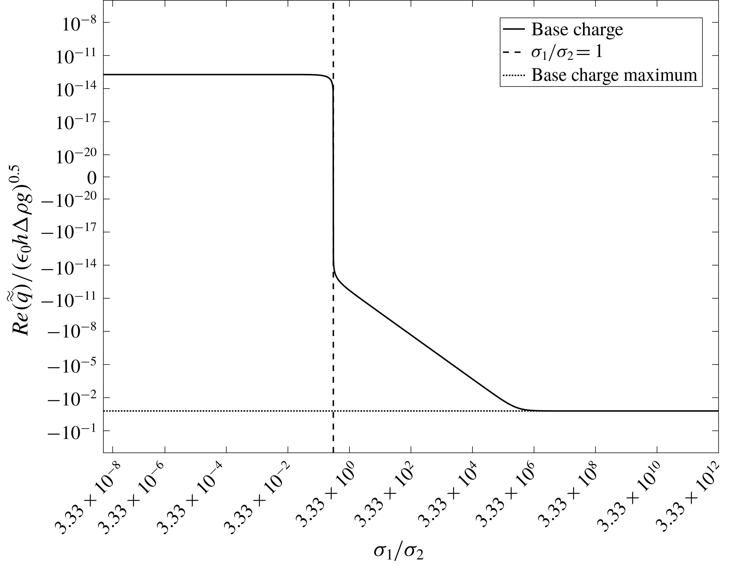
Utilizing a leaky dielectric model introduces multiple new parameters that can influence the system stability. We start our analysis by examining the effect of conductivity. For the purposes of the current work,
 $\unicode[STIX]{x1D70E}_{2}$
was set to a fixed value of
 $3\times 10^{-15}~\text{S}~\text{m}^{-1}$
and
 $\unicode[STIX]{x1D70E}_{1}$
was adjusted over a wide range. The first important result is the saturation of the base state charge density upon reaching a high value of
 $\unicode[STIX]{x1D70E}_{1}$
. Figure 6 shows the value of the real part of
 $\tilde{\tilde{q}}$
from (2.40) as a function of
 $\unicode[STIX]{x1D70E}_{1}$
. For low values of
 $\unicode[STIX]{x1D70E}_{1}$
, we observe an exponential dependence of
 $\tilde{\tilde{q}}$
on
 $\unicode[STIX]{x1D70E}_{1}$
. However, this trend vanishes upon reaching values of
 $\unicode[STIX]{x1D70E}_{1}\geqslant 10^{-8}$
, where a saturation of
 $\tilde{\tilde{q}}$
is observed beyond which increasing conductivity no longer strongly influences
 $\tilde{\tilde{q}}$
.
Effect of
 $\unicode[STIX]{x1D70E}_{1}$
on
 $q_{0}$
. An exponential dependence is observed for low values of
 $\unicode[STIX]{x1D70E}_{1}$
, but upon reaching
 $\unicode[STIX]{x1D70E}_{1}=10^{-8}$
,
 $q_{0}$
saturates and is no longer strongly affected by increasing
 $\unicode[STIX]{x1D70E}_{1}$
. Fluid parameters are the same as shown previously, assuming
 $\unicode[STIX]{x1D70E}_{2}=3\times 10^{-15}~\text{S}~\text{m}^{-1}$
and
 $\unicode[STIX]{x1D716}_{1}=\unicode[STIX]{x1D716}_{2}=1.00059$
.
 $A=D=5~\text{kV}$
and
 $\unicode[STIX]{x1D714}=25~\text{Hz}$
.

The term
 $\tilde{\tilde{q}}$
also exhibits a saturation in situations where
 $\unicode[STIX]{x1D70E}_{1}<\unicode[STIX]{x1D70E}_{2}$
. In fact, at the exact point of equality, shown by the dashed line in figure 6, the value of
 $\tilde{\tilde{q}}$
asymptotes and reverses sign. This is indicative that the sign of the base state charge is dependent on the initial orientation of the fluids with respect to their electrical conductivities. If the value of
 $\unicode[STIX]{x1D70E}_{2}$
were subsequently raised after lowering
 $\unicode[STIX]{x1D70E}_{1}$
to
 $3\times 10^{-15}$
, the base state charge would saturate with high
 $\unicode[STIX]{x1D70E}_{2}$
to the same value as shown for high
 $\unicode[STIX]{x1D70E}_{1}$
but with opposing sign, though this only occurs precisely when the permittivities of both fluids are equal.
It should be noted here that
 $\hat{q}$
exhibits similar behaviour, but saturates at a much lower
 $\unicode[STIX]{x1D70E}_{1}$
than
 $\tilde{\tilde{q}}$
. Here, the base state values of
 $\tilde{\tilde{q}}$
and
 $\hat{q}$
upon saturation can be accurately predicted by setting (2.15) and the
 $\unicode[STIX]{x1D713}_{2}$
portion of (2.41) equal to each other and solving for
 $q_{0}$
. This results in
 $$\begin{eqnarray}q_{0}=-\!\left(D-\frac{A}{2}(\text{e}^{\text{i}\unicode[STIX]{x1D714}t}+\text{e}^{-\text{i}\unicode[STIX]{x1D714}t})\right)\frac{\unicode[STIX]{x1D716}_{0}\unicode[STIX]{x1D716}_{2}}{h_{2}}\end{eqnarray}$$
which implies
 $$\begin{eqnarray}\displaystyle \left.\begin{array}{@{}c@{}}\displaystyle \hat{q}=-\frac{D\unicode[STIX]{x1D716}_{0}\unicode[STIX]{x1D716}_{2}}{h_{2}},\\ \displaystyle \tilde{\tilde{q}}=\frac{A\unicode[STIX]{x1D716}_{0}\unicode[STIX]{x1D716}_{2}}{2h_{2}},\end{array}\right\} & & \displaystyle\end{eqnarray}$$
which is shown by the dotted line in figure 6. Once
 $\tilde{\tilde{q}}$
and
 $\hat{q}$
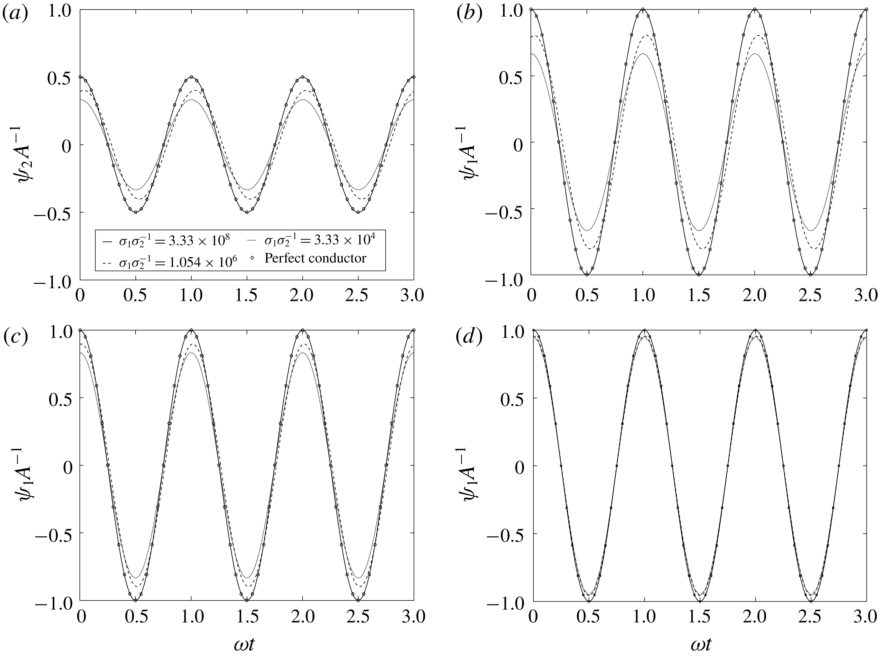
saturate, it is seen that the base state voltage profiles in both fluids yield the same results as the perfect conductor model. However, at
 $\unicode[STIX]{x1D70E}_{1}<10^{-8}$
, a departure between the voltage profiles is observed. The implications of this phenomenon are shown in figure 7 for
 $z$
values in the centre of each layer and at the interface.
Effect of
 $\unicode[STIX]{x1D70E}_{1}$
on the base state voltage profiles in the centre of the top fluid (a), at the interface (b) and in the centre of the bottom fluid (c). It is clearly seen that as
 $\unicode[STIX]{x1D70E}_{1}$
increases, the voltage profiles approach those of the perfect conductor model. Fluid properties and
 $\unicode[STIX]{x1D714}$
are equivalent to those in figure 6 and
 $D=0$
. (d) The same properties as (c), with the exception that
 $\unicode[STIX]{x1D716}_{1}=10$
. The base state voltage profiles saturate much more quickly with decreasing
 $\unicode[STIX]{x1D70E}_{1}$
if
 $\unicode[STIX]{x1D716}_{1}\gg \unicode[STIX]{x1D716}_{2}$
.

Thus, we can conclude that the maximum value of the base state charge density and also the maximum amplitude of the base state voltage drop across the fluids are given by those values which satisfy the perfect conductor model. It can also be shown that decreasing the conductivity of the bottom fluid much lower than that of the top fluid causes the same phenomena to occur, assuming that the perfect conductor model is re-derived with the conducting fluid on top. This behaviour is indicative that the leaky dielectric model will give similar results to the perfect conductor model, provided the conductivity of the bottom fluid is very high. This should come as no surprise, as this stipulation is the very assumption that leads to the simplifications made in the perfect conductor model case.
Another behaviour, shown in figure 7(d), is that the voltage profiles saturate to lower values very quickly with decreasing
 $\unicode[STIX]{x1D70E}_{1}$
if the permittivity ratio, i.e.
 $\unicode[STIX]{x1D716}_{1}/\unicode[STIX]{x1D716}_{2}$
is high. The behaviour is similar within the top fluid and at the interface and thus the results are omitted for brevity. This results in an insensitivity to conductivity of the base state voltage profiles, and ultimately the system stability. The saturation values are given by those which are derived for the perfect dielectric model, obtained by setting
 $q$
to zero in (2.36) and omitting (2.37).
Using the base state and corresponding perturbed state profiles, we now generate
 $A$
versus
 $k$
curves for the leaky dielectric model for comparison to those produced by the perfect conductor model. For high
 $\unicode[STIX]{x1D70E}_{1}$
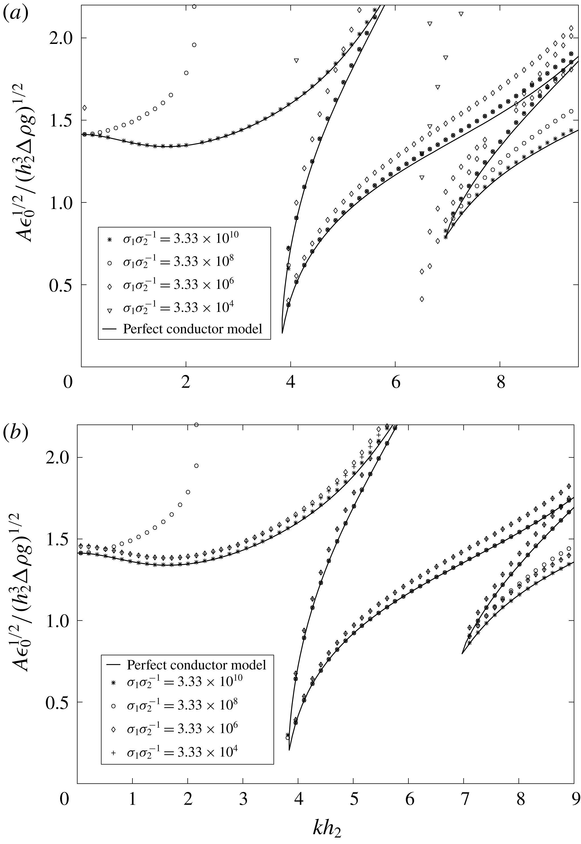
, as predicted, the leaky dielectric model yields results very similar to those seen in figure 3. However, upon lowering
 $\unicode[STIX]{x1D70E}_{1}$
, we find a quick departure from the perfect conductor model. Figure 8(a) shows the effect of conductivity on the system stability, along with the corresponding perfect conductor model results for comparison.
Stability thresholds for the leaky dielectric model assuming various conductivities for the bottom fluid. It is seen that a high conductivity will yield similar results to the perfect conductor model, but lowering the conductivity quickly causes a departure from this ideality.
 $\unicode[STIX]{x1D714}=25$
Hz and the fluid properties are the same as those given in figure 3(b), along with
 $\unicode[STIX]{x1D70E}_{2}=3\times 10^{-15}~\text{S}~\text{m}^{-1}$
and (a)
 $\unicode[STIX]{x1D716}_{1}=2$
or (b)
 $\unicode[STIX]{x1D716}_{1}=50$
.

Departure from the perfect conductor model
The departure in the Faraday tongues from the perfect conductor model arises quickly with decreasing conductivity of the bottom fluid. Typically, the stability tongues shift upward and to slightly lower wavenumber while maintaining their shapes. This behaviour is caused as the lower conductivity requires a higher imposed amplitude to generate the same interfacial stress due to voltage drops across the bulk. The exception to the rule can be seen in the case of
 $\unicode[STIX]{x1D70E}_{1}=10^{-8}~\text{S}~\text{m}^{-1}$
, where the second harmonic tongue decreases in threshold amplitude from the more conductive cases. This behaviour is presumably caused by the complex interaction between conductivity and permittivity, where terms multiplying higher orders of
 $A$
, not seen in the perfect conductor model, begin to grow (see (2.26) and (2.51)). Thus, slight destabilization can be observed by treating the fluids as leaky dielectrics, under particular constraints. Traces of this effect remain when
 $\unicode[STIX]{x1D70E}_{1}$
is further decreased, allowing the second harmonic tongue to remain lower than the first harmonic tongue. The first tongue rises dramatically with each decrease in
 $\unicode[STIX]{x1D70E}_{1}$
, as would be shown by a similar expression to (2.29) upon re-derivation using leaky dielectric fluids.
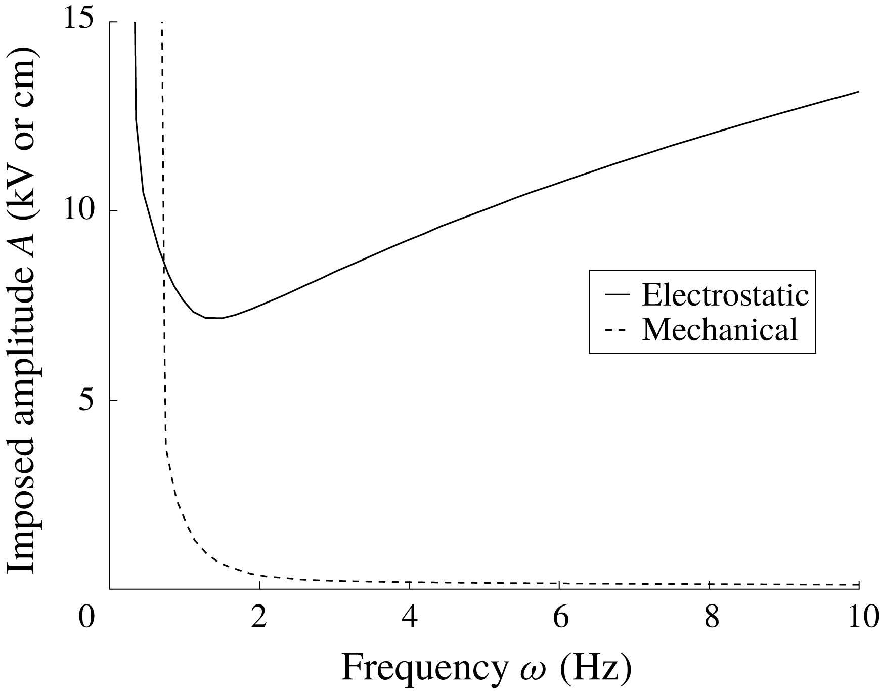
Relationship between critical amplitude and forcing frequency for electrostatically (solid) and mechanically (dashed) forced systems. The fluid parameters are given in table 1, with heights of 2.5 cm each. The imposed amplitude is measured in kV for the electrostatic case and cm for the mechanical case. The graph is presented unscaled because of the difference in the physical nature of the amplitudes.

The departure of the stability curves from the perfect conductor model behaves slightly differently if the permittivity of the bottom fluid is increased. In this case, an initial departure from the results of the perfect conductor is still observed with decreasing
 $\unicode[STIX]{x1D70E}_{1}$
. However, the solutions quickly saturate to a new state, where the problem becomes insensitive to
 $\unicode[STIX]{x1D70E}_{1}$
. This phenomenon occurs because of the saturation of the base state charge and voltage profiles, as seen in figure 7(d). The saturation approaches the solution to a stacked perfect dielectric system, and is shown in figure 8(b) for the same conditions as figure 8(a) with
 $\unicode[STIX]{x1D716}_{1}$
now set to 50.
Behaviour of
 $A$
with
$\unicode[STIX]{x1D714}$


Translating the
 $A$
versus
 $k$
stability plots as seen above into plots which relate the critical amplitude of oscillation to the parametric frequency is necessary for experimental validation. This procedure is done by generating a curve similar to that shown in figure 8(a) for a wide range of frequencies, and selecting the lowest unstable amplitude available at each of these frequencies. This critical amplitude, and the corresponding wavenumber, are that which will be seen in an experiment for a particular frequency. Generating this curve yields a smooth line which asymptotes to infinity as the frequency approaches zero, and in general decreases with increasing frequency. However, after a certain frequency, increased viscous damping acting on higher wavenumbers causes the curve to begin to rise and increase indefinitely. This is in stark contrast to the behaviour observed for mechanically forced Faraday instability, in which the curve never begins to rise with increasing frequency. (The behaviour in mechanically forced systems was incorrectly reported by Batson, Zoueshtiagh & Narayanan (Reference Batson, Zoueshtiagh and Narayanan2013a
) for low gravity predictions, and in fact never rises so long as any wavenumber is allowable.) Figure 9 shows a comparison between this behaviour in both electrostatically and mechanically forced systems.
This behaviour is a direct result of the distinct physics arising due to the electrostatic nature of the problem. In a mechanically oscillated system, the critical amplitude term is related to a critical acceleration given by
 $A\unicode[STIX]{x1D714}^{2}$
which multiplies the density difference between the fluids. The amplitude of acceleration is never encountered by itself, and thus one of the effects of increasing
 $\unicode[STIX]{x1D714}$
is to increase the acceleration term, which goes as
 $\unicode[STIX]{x1D714}^{2}$
. Since this happens, the stabilization from viscous dissipation is overwhelmed with increasing frequency, and the curve asymptotes monotonically. In the electrostatic case, however, the amplitude of voltage oscillation appears independent of frequency, as can be seen explicitly in (2.25). This means that increasing the frequency does not directly increase the terms containing
 $A$
, and thus viscous dissipation has the opportunity to overcome the typical decrease in threshold with increasing frequency.
Summary of fluid properties for the demonstration of critical amplitude dependence on frequency shown in figure 9. The electrical properties play no role in the mechanically forced calculation.

Another interesting consequence of the forcing is the impact of the
 $\unicode[STIX]{x0394}\unicode[STIX]{x1D70C}$
on the overall system stability. In particular, Faraday instability can only be excited in two-fluid mechanically forced systems with finite
 $\unicode[STIX]{x0394}\unicode[STIX]{x1D70C}$
values. Again, this is due to the nature of the amplitude term, which is only found in the form
 $A\unicode[STIX]{x1D714}^{2}\unicode[STIX]{x0394}\unicode[STIX]{x1D70C}$
. Naturally, this term vanishes as
 $\unicode[STIX]{x0394}\unicode[STIX]{x1D70C}$
disappears, and there is no possibility for Faraday instability to occur. In contrast, the amplitude term in electrostatically forced Faraday instability systems does not multiply
 $\unicode[STIX]{x0394}\unicode[STIX]{x1D70C}$
, and thus there is still possibility for destabilization when
 $\unicode[STIX]{x0394}\unicode[STIX]{x1D70C}$
is set to zero. One must be wary of low wavenumbers in this case if the desired instability is a standing wave, however, as the first tongue solution now shifts to lower amplitudes due to the absence of the gravitational term shown in (2.28). The ability to easily generate Faraday instability in systems with small
 $\unicode[STIX]{x0394}\unicode[STIX]{x1D70C}$
values is a definite benefit of electrostatic forcing to mechanical forcing in applications where intentionally exciting the instability could be beneficial to the process, such as microfluidic mixing enhancement (Amiroudine, Zoueshtiagh & Narayanan Reference Amiroudine, Zoueshtiagh and Narayanan2012).
3 Experimental validation of the theory
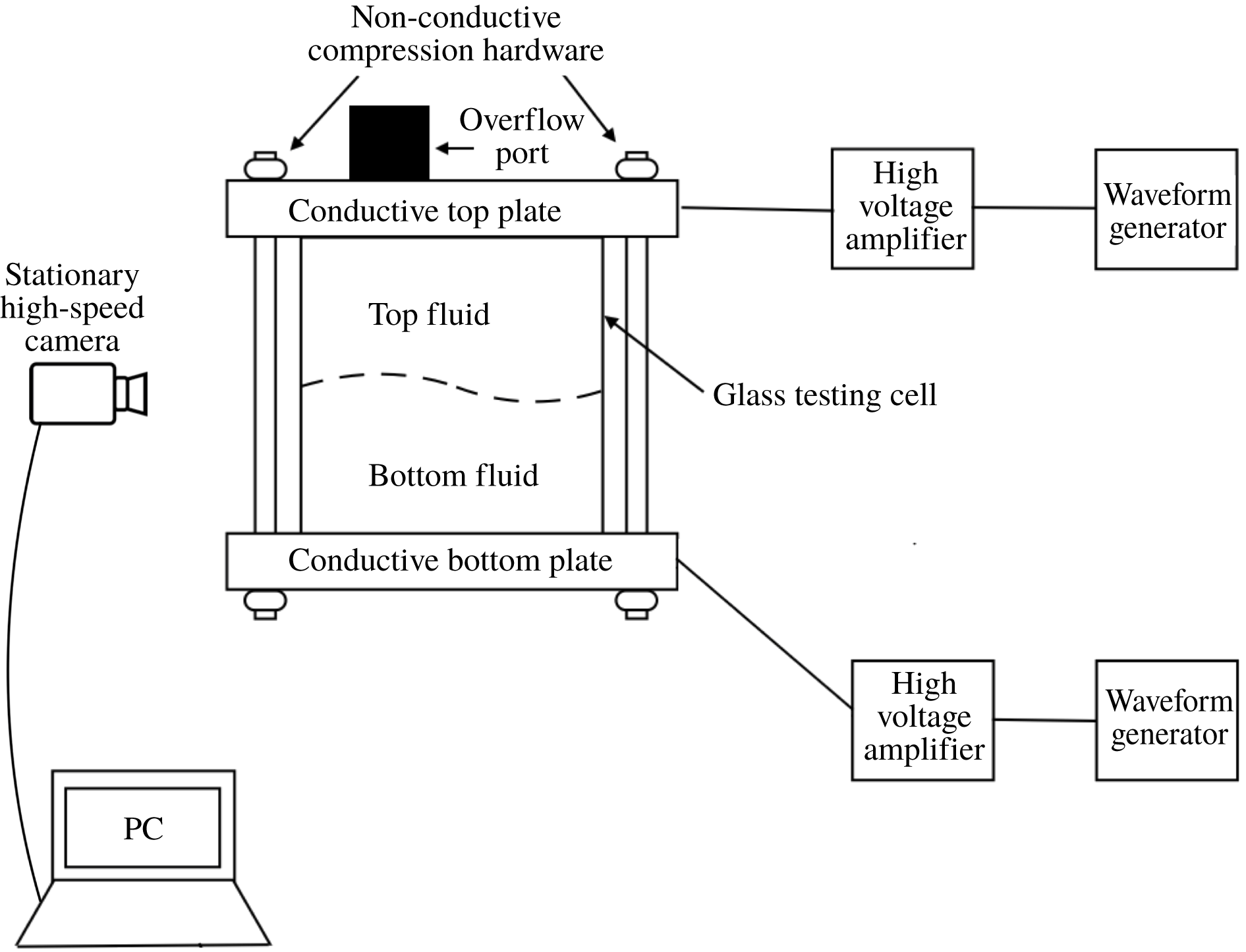
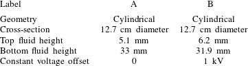
In order to verify the model, experiments were conducted using a two-fluid system axially constrained by two metallic electrodes, made of aluminium, and laterally bounded by glass walls. Though the testing geometry was laterally bounded, the distance between the walls was large, allowing for comparison to the laterally unbounded theory. Figure 10 shows a schematic of the experimental apparatus, and table 2 gives a summary of the geometry and operating conditions. It should be noted that the measurements within §§ 3 and 4 are reported in unscaled form to give a physical sense of the experimental parameters.
Assembled testing cell and experimental set-up. The geometry of choice is sealed between two conductive plates and secured with four non-conductive screws. The top and bottom plates are wired to high voltage amplifiers, and the voltages are controlled using independent signal generators. Backlighting allows for the clear visualization of the interface and any deflection using a high-speed camera.

Summary of the testing geometries and operating conditions. Two tests were conducted using a cylindrical geometry without a constant voltage offset (A) and with a constant voltage offset (B).

The testing geometry was constructed with top and bottom aluminium plates which enclose the testing cell. The cell itself was constructed from commercially available glass piping. The top and bottom plates were sealed around the testing cell through compression using Buna-N rubber seals and acrylic screws and wing nuts. An overflow port constructed from Delrin plastic was also threaded through the top plate to allow for filling of the cell. A two-fluid system was utilized for all of the experiments by filling the cell through the overflow port until there was direct contact between the upper fluid and the upper electrode without any additional air layer. This port also served to provide an additional source of the upper fluid in contact with the inner cell as well as space for the testing fluids to expand. This allowed experiments to be run over long time scales without air bubble generation within the cell. All of the hardware besides the top and bottom plates must be non-conductive for the apparatus to function properly.
Two electrodes were wired to high voltage amplifiers and WAVEFACTORY WF 1943A (top) and 1944A (bottom) signal generators, which were independently controllable by the user. Each electrode was capable of producing voltages up to
 $\pm$
10 kV. Frequencies in the millihertz to megahertz range were obtainable, though the experiments conducted for the current work utilized frequencies in the
 $0.5{-}10$
Hz range. The accuracy of the imposed oscillation frequency was
 $\pm$
0.0005 % and the accuracy of the amplitude varied based on the setpoint, but was typically
 $\pm$
3 % or better. The electrodes were connected to the top and bottom plates of the testing geometry using alligator clips and a high-speed camera was positioned at an angle slightly above a plane parallel to the interface to allow for viewing of the interface in its entirety. Typical experiments included an imposed AC oscillation with set amplitude and frequency on the bottom electrode, while simultaneously holding the upper electrode at a constant voltage.
The fluid choices were based on experimental considerations. In particular, it was found that one fluid needed to be much more conductive than the other in order to make the threshold experimentally obtainable. If both fluids were very non-conductive, then the resulting thresholds became too high to be generated. In addition, short circuits were observed if the amplitude was raised too high, resulting in the generation of bubbles and an automatic shutoff of the high voltage amplifiers for safety. Thus, the most repeatably usable system was ultra-pure water and 1.5 cSt silicone oil, with the majority of the total height being made of the water. The water heights tested were 33 mm and 31.9 mm with corresponding silicone oil heights of 5.1 mm and 6.2 mm, respectively. This allowed for a low critical threshold that was obtainable without inadvertently introducing short circuiting within apparatus.
For the geometries tested in these experiments, the side walls were machined to be far apart to mimic the unbounded nature of the theory. To determine the threshold of the instability, a forcing frequency was selected and an amplitude higher than the threshold was input to examine the responding Faraday waves. The amplitude was slowly decreased until the Faraday modes were no longer seen. This point was determined by measuring the harmonicity of the waves inside the cell. If any single harmonic wave (for
 $D=0$
) or subharmonic wave (for
 $D\neq 0$
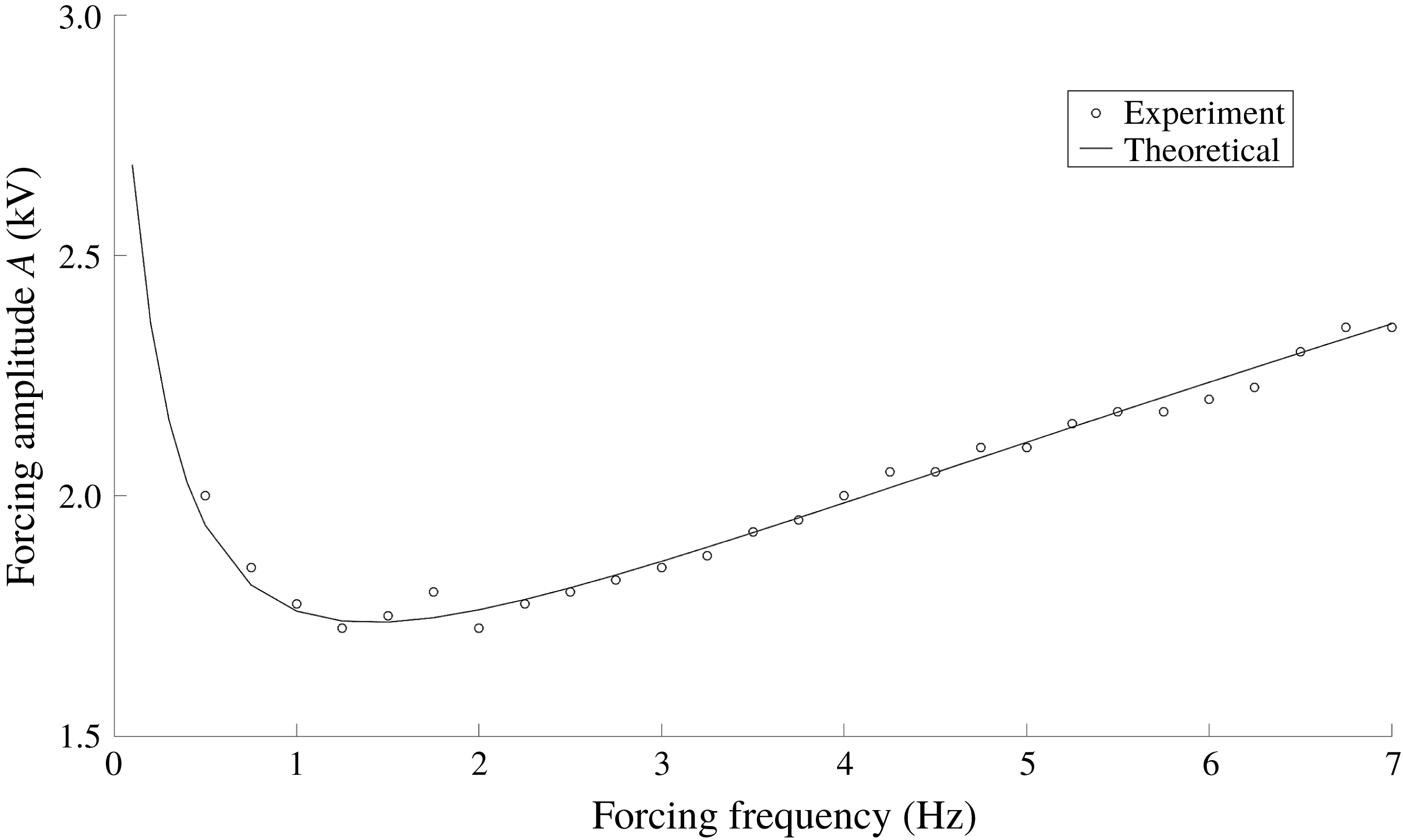
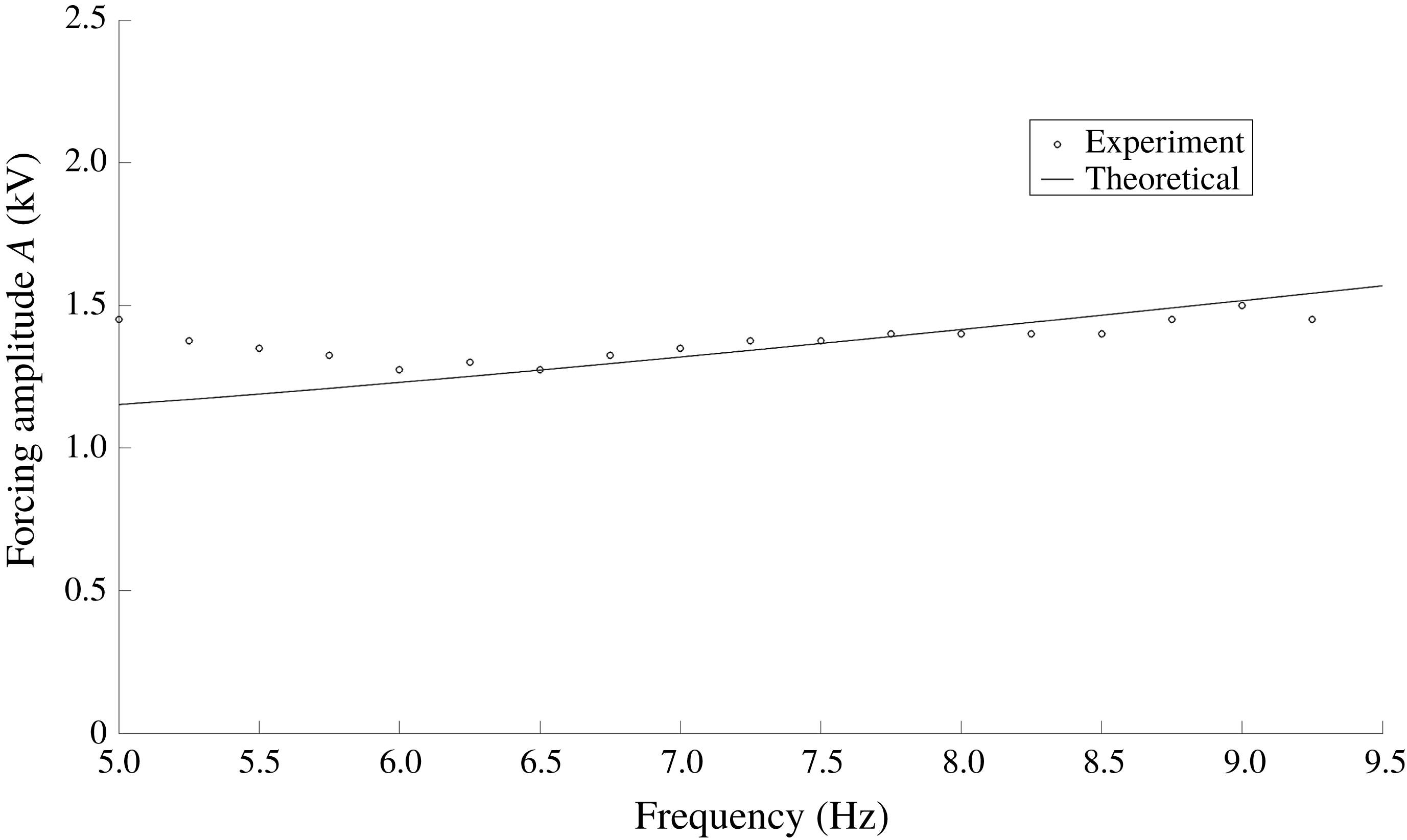
) was observed then the system was taken to be Faraday unstable. The gap between the stable and unstable amplitudes was decreased sequentially until adequate precision (typically 0.1 kV peak to peak) for the threshold amplitude was obtained. The standard time for each experiment was set to be three minutes unless the system became obviously unstable. If the instability did not present itself after three minutes of forcing time, then the tested amplitude was concluded to be within the stable range. As the experimental cells were large enough to behave as unbounded, discrete modes were not obtained during the experiments. Instead, multiple wavelengths were expressed after reaching the threshold for all of the tested frequencies. Due to the camera orientation, the curvature of the glass, and meniscus waves arising due to side wall non-idealities, we were unable to discern the wavelengths to any accuracy, and thus they are not reported. Figure 11 shows the theoretical curve and experimental results for Test A.
Comparison between theoretical and experimental thresholds for Test A. The model is able to capture the experimental threshold accurately over a large frequency range. Threshold amplitudes were measured to the nearest 0.05 kV.

For these experiments, the DC offset (
 $D$
) of the parametric forcing was set to zero. This results in base state meniscus waves that were twice harmonic with the imposed frequency. With an offset of zero, the lowest available Faraday instability tongue is harmonic with the imposed frequency. The agreement between the theory and experiment is excellent when utilizing this geometry and fluid combination. Definite distinction between unstable and stable amplitudes were easily observed with this geometry and operational parameter set. The minimum in the stability curve was exhibited experimentally and the overall behaviour of the theoretical stability curve was confirmed.
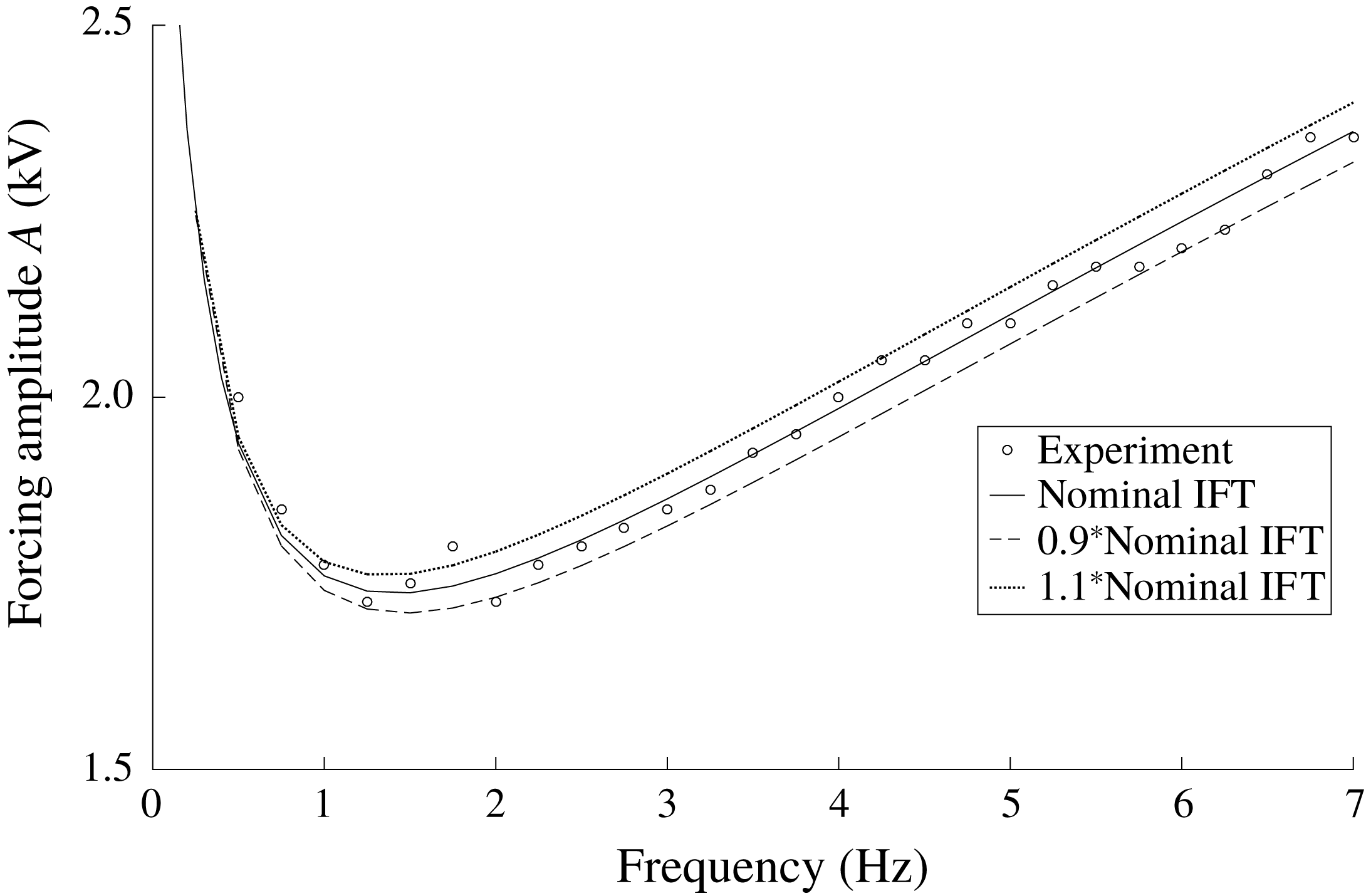
Figure 12 depicts the theoretical and experimentally determined threshold amplitudes for Test B, which utilized a non-zero voltage offset. This results in base state meniscus waves that were harmonic with the imposed frequency, and therefore the lowest available Faraday tongue is subharmonic.
Comparison between theoretical and experimental thresholds for Test B. The model is able to predict the instability threshold excellently at high frequency, but interfacial disturbances arising from the DC offset cause discrepancy at lower frequencies. Threshold amplitudes were measured to the nearest 0.05 kV.

As can be seen in figure 12, agreement between the theoretical predictions and experimental data is also reasonable when utilizing a non-zero voltage offset, though not to the same extent as the zero offset case. We conjecture that this is because of imperfections arising due to the presence of a meniscus, despite the fact that the container aspect ratio was large. It was observed that even if a pure DC forcing was imposed without an AC component, flow would ensue near the walls and this effect was accentuated by a superimposed AC. Understandably, this imperfection due to the meniscus did not manifest itself as significantly when the DC offset was absent, due to the high frequency of the imposed AC signals. The disturbance caused by the DC offset was seemingly magnified at lower frequency, and thus the threshold measurements were only accurately obtainable at higher frequencies. In addition, low frequency experiments offer comparable threshold amplitudes for both subharmonic and harmonic responses. These harmonic responses could compound the noise resulting from the DC offset, thus acting to drown out the subharmonic responses.
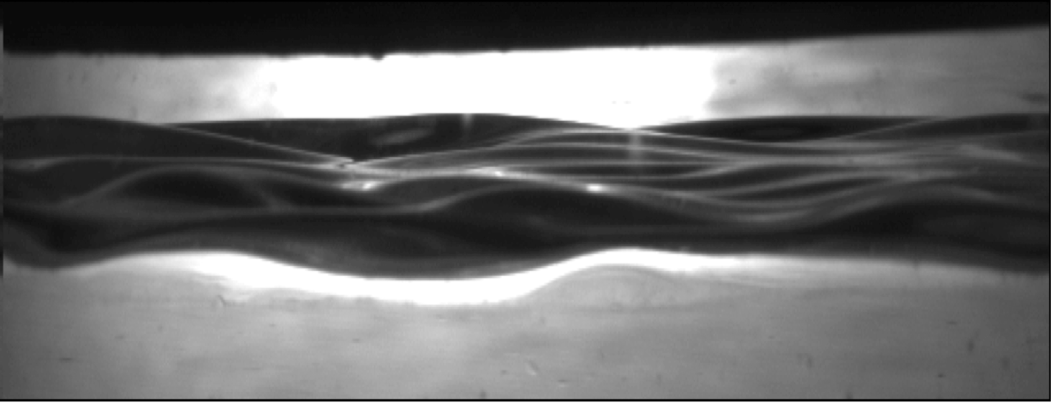
Despite these small discrepancies, the experimental data well support the predictions made by the theoretical model for these fluid systems. The agreement is typically best when no voltage offset is imposed. Figure 13 shows an example of Faraday waves obtained during Test A. It can clearly be seen that many wavelengths compete within the cell, but the resulting waveforms are proven to be a result of the Faraday instability due to their response frequency. A supplementary movie, available at https://doi.org/10.1017/jfm.2018.940, shows the temporal behaviour of a typical unstable interface.
Faraday waves obtained during Test A. The frequency and amplitude of forcing are 3.5 Hz and 2.5 kV, respectively. The photograph is taken during the portion of the response cycle with the largest interfacial deflection, and the applied amplitude exceeds the critical threshold.

4 Measurement of interfacial tension using electrostatically forced Faraday instability
In this section, we show that the electrostatically forced resonant instability is an excellent candidate for the measurement of interfacial tension between liquids, particularly if there is a substantial contrast between their electrical properties. Multiple means for measuring interfacial tension between liquids are currently employed, including both static and dynamic methods. Examples of static methods include the traditional pendant drop tensiometer and Wilhelmy plate (Adamson & Gast Reference Adamson and Gast1997), and examples of dynamic methods include the pulse-oscillation technique (Hyers & Rogers Reference Hyers and Rogers2008). The accurate measurement of interfacial tension is important to a variety of processes, including crystal growth (Schwabe Reference Schwabe1988), enhanced oil recovery techniques (Rosen et al. Reference Rosen, Wang, Shen and Zhu2005; Zhou, Das & Ellis Reference Zhou, Das and Ellis2016) and space welding (Workman & Kaukler Reference Workman and Kaukler1989; Fragomeni & Nunes Reference Fragomeni and Nunes2003).
The unique nature of electrostatic forcing allows for the imposition of a force which opposes gravity through the constant voltage component of the normal stress (see appendix A). Reduction of the effect of gravity allows interfacial tension to play a more dominant role on the system stability, and thus enables electrostatically forced Faraday instability to be used as a method of interfacial tension measurement. In order to test the accuracy of this measurement method, various interfacial tension values were assumed within the leaky dielectric model and curves of
 $A$
versus
 $\unicode[STIX]{x1D714}$
were computed. The curve with the closest fit to the experimental data allows us to deduce the interfacial tension between the fluids. Note that the experimental data were presented earlier in figure 11. Figure 14 now shows the same experimental data compared with various theoretical curves where different values of the interfacial tension are assumed.
Interfacial tension measurement for Si–oil and water system using electrostatic Faraday instability. The solid line represents the nominal interfacial tension, and clearly provides the best fit for the experimental data (
 $R^{2}=0.978$
). Testing properties are those given for figure 11.

As can be seen in the figure, the solid line produces the most accurate match of the experimental data. This is the line corresponding to the nominal interfacial tension between the testing fluids (0.045
 $\text{kg}~\text{s}^{-2}$
) measured using a KRÜSS DSA100 pendant drop tensiometer. Changing the interfacial tension within the model clearly impacts the predicted stability thresholds, and the effect is substantial enough to be seen experimentally. This study clearly shows that by using interfacial tension as an adjustable parameter within the model to match the experimental data, one would deduce an accurate interfacial tension between the two fluids. This is an important result, as it could potentially serve as a method for the measurement of interfacial tension in systems which behave as electrically conducting pairs such as gallium arsenide superposed by boron oxide, a system found in semiconductor crystal growth processes (Kumar & Subramanian Reference Kumar and Subramanian2015), whose interfacial tension measurement cannot be conveniently made using any of the conventional means. The method complements previous studies on the mechanically (Kumar Reference Kumar1999, Reference Kumar2002; Raynal, Kumar & Fauve Reference Raynal, Kumar and Fauve1999; Suman & Kumar Reference Suman and Kumar2008) and electrostatically (Espin et al.
Reference Espin, Corbett and Kumar2013) forced Faraday instabilities utilizing various viscoelastic fluids. The results from these studies suggest that the instability could possibly be harnessed as a characterization method for fluid rheological properties. Again, these types of novel characterization methods could prove valuable for systems exhibiting properties that preclude the use of conventional measurement methods.
5 Conclusions
The Faraday instability or resonant instability is studied theoretically and experimentally for electrostatically forced unconstrained systems. This work is the first to report theoretical and experimental observations of the effects of periodic electrostatic forcing on the physics of resonant instability for viscous fluids while accounting for charge dynamics at the interface. The study, which employs classical Floquet instability methods, reveals several results first from a perfect dielectric/perfect conductor model and then from a full leaky dielectric model, culminating in defining, validating experiments.
Multiple observations are made in this study, many of which are new and which arise from the model and the experiments that were conducted. First, it is seen theoretically that the resonant instability that is excited may lead to either subharmonic or harmonic responses depending on the value of the time-independent component of the voltage that is imposed on one of the horizontal bounding walls. These responses are in the shape of ‘tongues’ in a graph of imposed critical amplitude versus disturbance wavenumber. In particular, it is shown clearly that the subharmonic tongues observed only occur when a non-zero constant voltage offset is added to the oscillatory voltage imposed on the bottom axial wall. In addition, we show that the magnitude of this constant voltage offset strongly influences the shape of the stability tongues and their corresponding critical amplitude values. Second, it is observed that the quadratic nature of the forcing yields another instability tongue – one that can never occur in mechanically forced Faraday instability. This new tongue is entirely due to the time-independent component arising from the quadratic character of the Maxwell stress. Third, it is observed that for systems which exhibit very large conductivity ratios, the leaky dielectric model yields stability thresholds very similar to a simplified perfect conductor model. However, in systems with smaller conductivity ratios, distinct physics are obtained through the use of a leaky dielectric model. In particular, lowering the conductivity of the fluids causes the stability tongues to rise in critical amplitude and shift slightly toward lower wavenumbers. The solutions saturate quickly to the perfect dielectric solutions in the case that the permittivity ratio is also high. Fourth, it is observed that though there are commonalities between the mechanically and electrostatically forced Faraday instability, distinct physics is obtained in the case of electrostatic forcing. For example, an increase in the threshold amplitudes at higher frequencies is observed when utilizing electrostatic forcing, but is entirely absent in mechanical forcing. The electrostatic nature of the forcing also causes the response frequencies to differ from that obtained when utilizing mechanical forcing. These distinctions allow for additional control and manipulation of the electrostatic Faraday instability. Finally, it is concluded that electrostatic forcing, unlike mechanical forcing, can act to counter gravity in a fluid system that is stacked in a gravitationally stable configuration. This observation, in concert with detailed experiments that were conducted to validate the leaky dielectric model, lead us to a novel method to measure interfacial tension. This new method paves the way for new technology to measure this key interfacial property in systems of industrial significance where conventional means cannot be conveniently used.
Acknowledgements
Support is acknowledged from the National Science Foundation via a Graduate Research Fellowship under grant no. DGE-1315138. In addition, K.W. and R.N. acknowledge support from NSF 0968313, CASIS NNH11CD70A, NASA NNX17AL27G, NSF EAPSI 1514711 and Space Florida via the Florida Space Grant Consortium. S.M. acknowledges support from JSPS KAKENHI grant no. JP15H03925.
Supplementary movie
A supplementary movie is available at https://doi.org/10.1017/jfm.2018.940.
Appendix A. Derivation of the Yih model and the natural frequency when utilizing electrostatic forcing
We begin the re-derivation of the Yih (Reference Yih1968) model by considering a two-fluid system constrained axially between electrodes which impose an oscillatory voltage drop across the fluids, as shown in figure 1. The bottom fluid is considered as an inviscid perfect electrical conductor, and the top fluid is taken as an inviscid perfect dielectric. In this case, the voltage profile in the bottom fluid, i.e.
 $\unicode[STIX]{x1D713}_{1}$
is taken to be constant at
 $A\cos \unicode[STIX]{x1D714}t$
for all
 $z$
. The electrostatics in the top fluid are governed by Laplace’s equation as shown in § 2.1, and the hydrodynamics in the fluids are governed by the Euler equations coupled with the continuity equation:
 $$\begin{eqnarray}\displaystyle & \displaystyle \unicode[STIX]{x1D70C}_{j}\left(\frac{\unicode[STIX]{x2202}\boldsymbol{V}_{j}}{\unicode[STIX]{x2202}t}+\boldsymbol{V}_{j}\boldsymbol{\cdot }\unicode[STIX]{x1D735}\boldsymbol{V}_{j}\right)=-\unicode[STIX]{x1D735}P_{j}-\unicode[STIX]{x1D70C}_{j}g\boldsymbol{i}_{z}, & \displaystyle\end{eqnarray}$$
 $$\begin{eqnarray}\displaystyle & \displaystyle \unicode[STIX]{x1D735}\boldsymbol{\cdot }\boldsymbol{V}_{j}=0, & \displaystyle\end{eqnarray}$$
where
 $\boldsymbol{V}$
is the fluid velocity,
 $P$
is the pressure,
 $\unicode[STIX]{x1D70C}$
is the density,
 $g$
is gravitational acceleration and
 $j=1,2$
denotes the bottom and top fluid, respectively.
The equations are linearized about a quiescent, non-deflecting base state in the usual way by expanding the dependent variables as shown in (2.14). Applying these expansions to (2.1) and (A 1) yields the base state domain equations shown in (2.15) and (2.16), respectively.
Similarly, the perturbation of the domain equations yields (at first order)
 $$\begin{eqnarray}\displaystyle & \displaystyle \unicode[STIX]{x1D70C}_{j}\frac{\unicode[STIX]{x2202}\boldsymbol{V}_{j}^{\prime }}{\unicode[STIX]{x2202}t}=-\unicode[STIX]{x1D735}P_{j}^{\prime }, & \displaystyle\end{eqnarray}$$
 $$\begin{eqnarray}\displaystyle & \displaystyle \unicode[STIX]{x1D735}\boldsymbol{\cdot }\boldsymbol{V}_{j}^{\prime }=0 & \displaystyle\end{eqnarray}$$
and
 $$\begin{eqnarray}\unicode[STIX]{x1D6FB}^{2}\unicode[STIX]{x1D713}_{1}^{\prime }=0.\end{eqnarray}$$
Velocity is eliminated from the problem by taking
 $\unicode[STIX]{x1D735}\boldsymbol{\cdot }$
of each side of (A 3) and utilizing continuity to obtain
 $$\begin{eqnarray}0=\unicode[STIX]{x1D6FB}^{2}P_{j}^{\prime }.\end{eqnarray}$$
All the dependent variables are expanded as
 $$\begin{eqnarray}\unicode[STIX]{x1D719}^{\prime }(x,z,t)=\text{e}^{\text{i}kx}\tilde{\unicode[STIX]{x1D719}}(z,t),\end{eqnarray}$$
where
 $\unicode[STIX]{x1D719}$
is any dependent variable. This leads to the expressions for the pressure in both phases,
 $$\begin{eqnarray}0=\left(\frac{\unicode[STIX]{x2202}^{2}}{\unicode[STIX]{x2202}z^{2}}-k^{2}\right)\tilde{P}_{j},\end{eqnarray}$$
whose solutions take the form
 $$\begin{eqnarray}\tilde{P}_{j}=A_{j}\sinh (kz)+B_{j}\cosh (kz),\end{eqnarray}$$
as well as the equation and solution for the perturbed voltage profile given by (2.18) and
 $$\begin{eqnarray}\tilde{\unicode[STIX]{x1D713}}_{j}=C_{j}\sinh (kz)+D_{j}\cosh (kz).\end{eqnarray}$$
No-penetration conditions, i.e.
 $\tilde{\boldsymbol{V}}_{z,j}=0$
, are imposed at both the bounding walls, resulting in
 $$\begin{eqnarray}\left.\begin{array}{@{}c@{}}\displaystyle \frac{\unicode[STIX]{x2202}\tilde{P}_{2}}{\unicode[STIX]{x2202}z}=0\quad \text{at }z=h_{2},\\ \displaystyle \frac{\unicode[STIX]{x2202}\tilde{P}_{1}}{\unicode[STIX]{x2202}z}=0\quad \text{at }z=-h_{1}\end{array}\right\}\end{eqnarray}$$
after substitution of these conditions into (A 3).
The usual kinematic condition is applied at the interface,
 $$\begin{eqnarray}\tilde{W}_{j}=\frac{\text{d}\tilde{\unicode[STIX]{x1D701}}}{\text{d}t},\end{eqnarray}$$
which after substitution into (A 3) yields
 $$\begin{eqnarray}\unicode[STIX]{x1D70C}_{j}\frac{\text{d}^{2}\tilde{\unicode[STIX]{x1D701}}}{\text{d}t^{2}}=-\frac{\unicode[STIX]{x2202}\tilde{P}_{j}}{\unicode[STIX]{x2202}z}.\end{eqnarray}$$
The unknown coefficients in (A 9) are determined in terms of
 $\text{d}^{2}\tilde{\unicode[STIX]{x1D701}}/\text{d}t^{2}$
using (A 13) and (A 11), yielding
 $$\begin{eqnarray}\left.\begin{array}{@{}c@{}}\displaystyle \tilde{P}_{1}=-\frac{\unicode[STIX]{x1D70C}_{1}}{k}\frac{\text{d}^{2}\tilde{\unicode[STIX]{x1D701}}}{\text{d}t^{2}}[\sinh (kz)-\coth (-kh_{1})\cosh (kz)],\\ \displaystyle \tilde{P}_{2}=-\frac{\unicode[STIX]{x1D70C}_{2}}{k}\frac{\text{d}^{2}\tilde{\unicode[STIX]{x1D701}}}{\text{d}t^{2}}[\sinh (kz)-\coth (kh_{2})\cosh (kz)].\end{array}\right\}\end{eqnarray}$$
The problem is closed using the jump momentum balance at order ‘
 $^{\prime }$
’,
 $$\begin{eqnarray}P_{2}^{\prime }-P_{1}^{\prime }+\unicode[STIX]{x1D701}^{\prime }\left(\frac{\text{d}P_{2}^{0}}{\text{d}z}-\frac{\text{d}P_{1}^{0}}{\text{d}z}\right)=-\unicode[STIX]{x1D6FE}k^{2}\unicode[STIX]{x1D701}+k\unicode[STIX]{x1D702}(D^{2}-2DA\cos \unicode[STIX]{x1D714}t+\cos ^{2}\unicode[STIX]{x1D714}t)\unicode[STIX]{x1D701}^{\prime },\end{eqnarray}$$
where
 $\unicode[STIX]{x1D702}=k\unicode[STIX]{x1D716}_{2}\unicode[STIX]{x1D716}_{0}\coth kh_{2}/h_{2}^{2}$
, which upon inserting the pressure expressions and expanding using (A 7) yields
 $$\begin{eqnarray}\frac{\text{d}^{2}\tilde{\unicode[STIX]{x1D701}}}{\text{d}t^{2}}+\frac{((\unicode[STIX]{x1D70C}_{2}-\unicode[STIX]{x1D70C}_{1})k-\unicode[STIX]{x1D6FE}k^{3})}{\unicode[STIX]{x1D70C}_{2}\coth kh_{2}+\unicode[STIX]{x1D70C}_{1}\coth kh_{1}}\tilde{\unicode[STIX]{x1D701}}+\frac{k\unicode[STIX]{x1D702}(D^{2}-2DA\cos \unicode[STIX]{x1D714}t+A^{2}\cos ^{2}\unicode[STIX]{x1D714}t)}{\unicode[STIX]{x1D70C}_{2}\coth kh_{2}+\unicode[STIX]{x1D70C}_{1}\coth kh_{1}}\tilde{\unicode[STIX]{x1D701}}=0,\end{eqnarray}$$
which can be cast into the form of the Mathieu equation
 $$\begin{eqnarray}\frac{\text{d}^{2}\tilde{\unicode[STIX]{x1D701}}}{\text{d}\unicode[STIX]{x1D70F}^{2}}+(p-2q\cos (2\unicode[STIX]{x1D70F}))\tilde{\unicode[STIX]{x1D701}}=0\end{eqnarray}$$
upon the transformations
 $$\begin{eqnarray}\left.\begin{array}{@{}c@{}}\displaystyle D=-A\cos \unicode[STIX]{x1D714}t,\\ \displaystyle \unicode[STIX]{x1D70F}=\unicode[STIX]{x1D714}t,\\ \displaystyle \unicode[STIX]{x1D70E}_{0}^{2}=\frac{((\unicode[STIX]{x1D70C}_{2}-\unicode[STIX]{x1D70C}_{1})k-\unicode[STIX]{x1D6FE}k^{3})}{\unicode[STIX]{x1D70C}_{2}\coth kh_{2}+\unicode[STIX]{x1D70C}_{1}\coth kh_{1}},\\ \displaystyle \unicode[STIX]{x1D6FD}=\frac{2A^{2}k^{2}\unicode[STIX]{x1D716}_{2}\unicode[STIX]{x1D716}_{0}\coth kh_{2}}{h_{2}^{2}(\unicode[STIX]{x1D70C}_{2}\coth kh_{2}+\unicode[STIX]{x1D70C}_{1}\coth kh_{1})},\\ \displaystyle p=\frac{\unicode[STIX]{x1D70E}_{0}^{2}+\unicode[STIX]{x1D6FD}}{\unicode[STIX]{x1D714}^{2}},\\ \displaystyle q=\frac{\unicode[STIX]{x1D6FD}}{2\unicode[STIX]{x1D714}^{2}}.\end{array}\right\}\end{eqnarray}$$
The natural frequency for an electrostatically forced inviscid two-fluid system can be obtained by first setting
 $A=0$
in (A 16) and further expanding using
 $$\begin{eqnarray}\tilde{\unicode[STIX]{x1D719}}(z,t)=\text{e}^{\unicode[STIX]{x1D70E}t}\hat{\unicode[STIX]{x1D719}}(z),\end{eqnarray}$$
which yields
 $$\begin{eqnarray}\unicode[STIX]{x1D70E}^{2}=-\frac{\left((\unicode[STIX]{x1D70C}_{1}-\unicode[STIX]{x1D70C}_{2})gk-{\displaystyle \frac{\unicode[STIX]{x1D716}_{2}\unicode[STIX]{x1D716}_{0}\coth kh_{2}}{h_{2}^{2}}}D^{2}k^{2}+\unicode[STIX]{x1D6FE}k^{3}\right)}{\unicode[STIX]{x1D70C}_{2}\coth kh_{2}+\unicode[STIX]{x1D70C}_{1}\coth kh_{1}},\end{eqnarray}$$
where
 $\unicode[STIX]{x1D70E}^{2}$
is the natural frequency. It should be noted that the modification to the natural frequency also exists with pure oscillatory forcing (i.e.
 $D=0$
) due to the
 $A/2$
arising from the application of the double angle formula.
In the absence of electrostatic forcing, the usual natural frequency for a stacked fluid system is comprised of gravitational and interfacial tension contributions, and is given by
 $\unicode[STIX]{x1D70E}_{0}^{2}$
in (A 18). These terms are also present within
 $\unicode[STIX]{x1D70E}^{2}$
, along with a modification term due to the Maxwell stress. Due to the fluid orientation, this modification term opposes the gravity and surface tension terms. If the conductive fluid had been located on the top, with all other parameters being equal, the term would have switched signs and acted in conjunction with the typical mechanical terms. Since the nature of Faraday instability revolves around the natural frequency, this is an extremely useful result. In mechanically forced Faraday instability calculations, when using typical density and interfacial tension values, the resulting stability curves are highly independent of the interfacial tension, allowing for order of magnitude changes to the interfacial tension with negligible impact to the system stability. In electrostatically forced Faraday instability, however, tailoring the imposed
 $D$
value and geometry (
 $k$
) to oppose gravity can begin to highlight the importance of interfacial tension on the stability thresholds. This can, as shown in § 4, allow for the measurement of interfacial tension using electrostatically forced Faraday instability for certain fluid combinations.
Appendix B. Derivation for the velocity profiles in terms of
$\unicode[STIX]{x1D701}_{n}$

The theoretical model used for the hydrodynamics in the perfect conductor model is obtained through linear stability analysis, following closely to the model derived by Kumar & Tuckerman (Reference Kumar and Tuckerman1994) with additional Maxwell stress terms within the total stress tensor (see (2.11)). A horizontally infinite two-fluid system is considered, and the hydrodynamics in both fluids are governed by (2.4)–(2.10). It is important to note here the absence of the
 $\unicode[STIX]{x1D70C}_{j}A\unicode[STIX]{x1D714}^{2}\cos \unicode[STIX]{x1D714}t$
term from the right-hand side of (2.4) which is present in mechanically forced Faraday instability problems as a result of adopting a moving reference frame.
These equations are linearized about a quiescent, non-deflecting base state by expanding the dependent variables as shown in (2.14). Applying the expansions yields the base state domain equation
 $$\begin{eqnarray}\frac{\unicode[STIX]{x2202}P_{0_{j}}}{\unicode[STIX]{x2202}z}=-\unicode[STIX]{x1D70C}_{j}g\end{eqnarray}$$
and the perturbed domain equations
 $$\begin{eqnarray}\left.\begin{array}{@{}c@{}}\displaystyle \unicode[STIX]{x1D70C}_{j}\frac{\unicode[STIX]{x2202}\boldsymbol{V}_{j}^{\prime }}{\unicode[STIX]{x2202}t}=-\unicode[STIX]{x1D735}P_{j}^{\prime }+\unicode[STIX]{x1D707}_{j}\unicode[STIX]{x1D6FB}^{2}\boldsymbol{V}_{j}^{\prime },\\ \displaystyle \unicode[STIX]{x1D735}\boldsymbol{\cdot }\boldsymbol{V}_{j}^{\prime }=0.\end{array}\right\}\end{eqnarray}$$
The double curl is applied to (B 2) to eliminate pressure along with the continuity equation, resulting in
 $$\begin{eqnarray}\unicode[STIX]{x1D70C}_{j}\unicode[STIX]{x2202}t\unicode[STIX]{x1D6FB}^{2}\boldsymbol{V}_{j}^{\prime }=\unicode[STIX]{x1D707}_{j}\unicode[STIX]{x1D6FB}^{4}\boldsymbol{V}_{j}^{\prime }.\end{eqnarray}$$
Equation (2.17) is then used to separate variables, resulting in the final perturbed domain equation and its accompanying boundary conditions (dropping hats)
 $$\begin{eqnarray}\left(\unicode[STIX]{x1D70E}+\text{i}(\unicode[STIX]{x1D6FC}+n\unicode[STIX]{x1D714})-\unicode[STIX]{x1D708}_{j}\left(\frac{\text{d}^{2}}{\text{d}z^{2}}-k^{2}\right)\right)\left(\frac{\text{d}^{2}}{\text{d}z^{2}}-k^{2}\right)W_{nj}=0\end{eqnarray}$$
and
 $$\begin{eqnarray}\left.\begin{array}{@{}c@{}}\displaystyle W_{n1}=0\quad \text{at }z=-h_{1},\\ \displaystyle \frac{\text{d}W_{n1}}{\text{d}z}=0\quad \text{at }z=-h_{1},\\ \displaystyle W_{n2}=0\quad \text{at }z=h_{2},\\ \displaystyle \frac{\text{d}W_{n2}}{\text{d}z}=0\quad \text{at }z=h_{2}\end{array}\right\}\end{eqnarray}$$
along with the corresponding interfacial conditions at
 $z=0$
,
 $$\begin{eqnarray}\left.\begin{array}{@{}c@{}}W_{n1}=W_{n2},\\ \displaystyle \frac{\text{d}W_{n1}}{\text{d}z}=\frac{\text{d}W_{n2}}{\text{d}z},\\ \displaystyle \unicode[STIX]{x1D707}_{1}\left(\frac{\text{d}^{2}}{\text{d}z^{2}}+k^{2}\right)W_{n1}=\unicode[STIX]{x1D707}_{2}\left(\frac{\text{d}^{2}}{\text{d}z^{2}}+k^{2}\right)W_{n2},\\ \displaystyle (\unicode[STIX]{x1D70E}+\text{i}(\unicode[STIX]{x1D6FC}+n\unicode[STIX]{x1D714}))\unicode[STIX]{x1D701}_{n}=W_{n1},\end{array}\right\}\end{eqnarray}$$
where
 $W$
is the
 $z$
-component of the perturbed velocity. Equation (B 4) is an ordinary differential equation, whose solution takes the form
 $$\begin{eqnarray}W_{nj}=A_{nj}\text{e}^{kz}+B_{nj}\text{e}^{-kz}+C_{nj}\text{e}^{q_{n}z}+D_{nj}\text{e}^{-q_{n}z},\end{eqnarray}$$
where
 $q_{n}=\sqrt{(\unicode[STIX]{x1D70E}+\text{i}(\unicode[STIX]{x1D6FC}+n\unicode[STIX]{x1D714}))/\unicode[STIX]{x1D708}_{j}+k^{2}}$
. It should be noted that when
 $q_{n}=k$
, the solution instead takes the form
 $$\begin{eqnarray}W_{nj}=A_{nj}\text{e}^{kz}+B_{nj}\text{e}^{-kz}+C_{nj}z\text{e}^{kz}+D_{nj}z\text{e}^{-kz}.\end{eqnarray}$$
All the unknown coefficients are then calculated by casting the system of equations into matrix form and solving via inversion. Expressions for the velocities in both fluids are now known in terms of
 $\unicode[STIX]{x1D701}_{n}$
. The remaining step is to solve the eigenvalue problem derived from the normal component of the stress balance, which ultimately governs the stability of the system:
 $$\begin{eqnarray}\left[\left[-\!\left(P^{\prime }+\unicode[STIX]{x1D701}^{\prime }\frac{\text{d}P_{0}}{\text{d}z}\right)+2\unicode[STIX]{x1D707}_{j}\frac{\text{d}W_{j}}{\text{d}z}\right]\right]+([[\unicode[STIX]{x1D64F}^{Maxwell}\boldsymbol{\cdot }\boldsymbol{n}]]\boldsymbol{\cdot }\boldsymbol{n})^{\prime }=-\unicode[STIX]{x1D6FE}\unicode[STIX]{x1D6FB}_{H}^{2}\unicode[STIX]{x1D701}^{\prime }.\end{eqnarray}$$
Applying
 $\unicode[STIX]{x1D6FB}_{H}^{2}\cdot$
to this equation, and substituting the base state pressure term given by (B 1), yields
 $$\begin{eqnarray}\left[\left[-\unicode[STIX]{x1D6FB}_{H}^{2}P^{\prime }+\unicode[STIX]{x1D6FB}_{H}^{2}(\unicode[STIX]{x1D70C}_{j}g)\unicode[STIX]{x1D701}^{\prime }+2\unicode[STIX]{x1D707}_{j}\unicode[STIX]{x1D6FB}_{H}^{2}\frac{\text{d}W_{j}}{\text{d}z}\right]\right]+\unicode[STIX]{x1D6FB}_{H}^{2}([[\unicode[STIX]{x1D64F}^{Maxwell}\boldsymbol{\cdot }\boldsymbol{n}]]\boldsymbol{\cdot }\boldsymbol{n})^{\prime }=-\unicode[STIX]{x1D6FE}\unicode[STIX]{x1D6FB}_{H}^{4}\unicode[STIX]{x1D701}^{\prime }.\end{eqnarray}$$
An expression for
 $\unicode[STIX]{x1D6FB}_{H}^{2}P^{\prime }$
is obtained by combining the continuity equation with
 $\unicode[STIX]{x1D735}_{H}\cdot$
(B 2):
 $$\begin{eqnarray}\unicode[STIX]{x1D6FB}_{H}^{2}P_{j}^{\prime }=\left(\unicode[STIX]{x1D70C}_{j}\frac{\unicode[STIX]{x2202}}{\unicode[STIX]{x2202}t}-\unicode[STIX]{x1D707}_{j}\unicode[STIX]{x1D6FB}^{2}\right)\frac{\unicode[STIX]{x2202}W_{j}}{\unicode[STIX]{x2202}z},\end{eqnarray}$$
which upon substitution into (B 10) and expanding variables using (2.17) yields
 $$\begin{eqnarray}\left[\left[\unicode[STIX]{x1D70C}_{j}(\unicode[STIX]{x1D70E}+\text{i}(\unicode[STIX]{x1D6FC}+n\unicode[STIX]{x1D714}))\frac{\unicode[STIX]{x2202}W_{nj}}{\unicode[STIX]{x2202}z}-\unicode[STIX]{x1D707}_{j}\frac{\text{d}^{3}W_{nj}}{\text{d}z^{3}}+k^{2}\unicode[STIX]{x1D70C}_{j}g\unicode[STIX]{x1D701}_{n}+3\unicode[STIX]{x1D707}_{j}k^{2}\frac{\text{d}W_{nj}}{\text{d}z}\right]\right]=\unicode[STIX]{x1D6FE}k^{4}\unicode[STIX]{x1D701}_{n}-k^{2}\unicode[STIX]{x1D70F}^{Maxwell}.\end{eqnarray}$$
Rearranging (B 12) leads to (2.22), after which the derivation continues in § 2.1.
Appendix C. Expanded matrices for the final eigenvalue problems
The matrices necessary to solve the final eigenvalue problem shown in § 2.1 are constructed separately for the cases of
 $\unicode[STIX]{x1D6FC}=0$
and
 $\unicode[STIX]{x1D6FC}=\unicode[STIX]{x1D714}/2$
. This results in
 $$\begin{eqnarray}\displaystyle & \displaystyle \bar{\unicode[STIX]{x1D63D}}=\left[\begin{array}{@{}cccccccccc@{}}B_{0}^{r} & -B_{0}^{i} & 0 & 0 & 0 & 0 & 0 & 0 & 0 & 0\\ B_{0}^{i} & B_{0}^{r} & 0 & 0 & 0 & 0 & 0 & 0 & 0 & 0\\ 0 & 0 & B_{1}^{r} & -B_{1}^{i} & 0 & 0 & 0 & 0 & 0 & 0\\ 0 & 0 & B_{1}^{i} & B_{1}^{r} & 0 & 0 & 0 & 0 & 0 & 0\\ 0 & 0 & 0 & 0 & \ddots & \ddots & 0 & 0 & 0 & 0\\ 0 & 0 & 0 & 0 & \ddots & \ddots & 0 & 0 & 0 & 0\\ 0 & 0 & 0 & 0 & 0 & 0 & B_{n-1}^{r} & -B_{n-1}^{i} & 0 & 0\\ 0 & 0 & 0 & 0 & 0 & 0 & B_{n-1}^{i} & B_{n-1}^{r} & 0 & 0\\ 0 & 0 & 0 & 0 & 0 & 0 & 0 & 0 & B_{n}^{r} & -B_{n}^{i}\\ 0 & 0 & 0 & 0 & 0 & 0 & 0 & 0 & B_{n}^{i} & B_{n}^{r}\\ \end{array}\right], & \displaystyle\end{eqnarray}$$
 $$\begin{eqnarray}\displaystyle & \displaystyle \bar{\unicode[STIX]{x1D701}}=\left[\begin{array}{@{}c@{}}\unicode[STIX]{x1D701}_{0}^{r}\\ \unicode[STIX]{x1D701}_{0}^{i}\\ \unicode[STIX]{x1D701}_{1}^{r}\\ \unicode[STIX]{x1D701}_{1}^{i}\\ \vdots \\ \vdots \\ \unicode[STIX]{x1D701}_{n-1}^{r}\\ \unicode[STIX]{x1D701}_{n-1}^{i}\\ \unicode[STIX]{x1D701}_{n}^{r}\\ \unicode[STIX]{x1D701}_{n}^{i}\\ \end{array}\right], & \displaystyle\end{eqnarray}$$
 $$\begin{eqnarray}\displaystyle & \displaystyle \bar{\unicode[STIX]{x1D63E}}=C\left[\begin{array}{@{}cccccccccc@{}}1 & 0 & 1 & 0 & 0 & 0 & 0 & 0 & 0 & 0\\ 0 & -1 & 0 & 1 & 0 & 0 & 0 & 0 & 0 & 0\\ 1 & 0 & 0 & 0 & 1 & 0 & 0 & 0 & 0 & 0\\ 0 & 1 & 0 & 0 & 0 & 1 & 0 & 0 & 0 & 0\\ 0 & 0 & \ddots & 0 & 0 & 0 & \ddots & 0 & 0 & 0\\ 0 & 0 & 0 & \ddots & 0 & 0 & 0 & \ddots & 0 & 0\\ 0 & 0 & 0 & 0 & 1 & 0 & 0 & 0 & 1 & 0\\ 0 & 0 & 0 & 0 & 0 & 1 & 0 & 0 & 0 & 1\\ 0 & 0 & 0 & 0 & 0 & 0 & 1 & 0 & 0 & 0\\ 0 & 0 & 0 & 0 & 0 & 0 & 0 & 1 & 0 & 0\\ \end{array}\right] & \displaystyle\end{eqnarray}$$
for
 $\unicode[STIX]{x1D6FC}=\unicode[STIX]{x1D714}/2$
, or
 $$\begin{eqnarray}\bar{\unicode[STIX]{x1D63E}}=C\left[\begin{array}{@{}cccccccccc@{}}0 & 0 & 2 & 0 & 0 & 0 & 0 & 0 & 0 & 0\\ 0 & 0 & 0 & 0 & 0 & 0 & 0 & 0 & 0 & 0\\ 1 & 0 & 0 & 0 & 1 & 0 & 0 & 0 & 0 & 0\\ 0 & 1 & 0 & 0 & 0 & 1 & 0 & 0 & 0 & 0\\ 0 & 0 & \ddots & 0 & 0 & 0 & \ddots & 0 & 0 & 0\\ 0 & 0 & 0 & \ddots & 0 & 0 & 0 & \ddots & 0 & 0\\ 0 & 0 & 0 & 0 & 1 & 0 & 0 & 0 & 1 & 0\\ 0 & 0 & 0 & 0 & 0 & 1 & 0 & 0 & 0 & 1\\ 0 & 0 & 0 & 0 & 0 & 0 & 1 & 0 & 0 & 0\\ 0 & 0 & 0 & 0 & 0 & 0 & 0 & 1 & 0 & 0\\ \end{array}\right]\end{eqnarray}$$
for
 $\unicode[STIX]{x1D6FC}=0$
and
 $$\begin{eqnarray}\bar{\unicode[STIX]{x1D640}}=E\left[\begin{array}{@{}cccccccccc@{}}2 & 0 & 1 & 0 & 1 & 0 & 0 & 0 & 0 & 0\\ 0 & 1 & 0 & -1 & 0 & 1 & 0 & 0 & 0 & 0\\ 1 & 0 & 2 & 0 & 0 & 0 & 1 & 0 & 0 & 0\\ 0 & -1 & 0 & 2 & 0 & 0 & 0 & 1 & 0 & 0\\ 1 & 0 & 0 & 0 & 2 & 0 & 0 & 0 & 1 & 0\\ 0 & \ddots & 0 & 0 & 0 & \ddots & 0 & 0 & 0 & \ddots \\ 0 & 0 & 1 & 0 & 0 & 0 & 2 & 0 & 0 & 0\\ 0 & 0 & 0 & 1 & 0 & 0 & 0 & 2 & 0 & 0\\ 0 & 0 & 0 & 0 & 1 & 0 & 0 & 0 & 2 & 0\\ 0 & 0 & 0 & 0 & 0 & 1 & 0 & 0 & 0 & 2\\ \end{array}\right]\end{eqnarray}$$
for
 $\unicode[STIX]{x1D6FC}=(\unicode[STIX]{x1D714}/2)$
, or
 $$\begin{eqnarray}\bar{\unicode[STIX]{x1D640}}=E\left[\begin{array}{@{}cccccccccc@{}}2 & 0 & 0 & 0 & 2 & 0 & 0 & 0 & 0 & 0\\ 0 & 2 & 0 & 0 & 0 & 0 & 0 & 0 & 0 & 0\\ 0 & 0 & 3 & 0 & 0 & 0 & 1 & 0 & 0 & 0\\ 0 & 0 & 0 & 1 & 0 & 0 & 0 & 1 & 0 & 0\\ 1 & 0 & 0 & 0 & 2 & 0 & 0 & 0 & 1 & 0\\ 0 & \ddots & 0 & 0 & 0 & \ddots & 0 & 0 & 0 & \ddots \\ 0 & 0 & 1 & 0 & 0 & 0 & 2 & 0 & 0 & 0\\ 0 & 0 & 0 & 1 & 0 & 0 & 0 & 2 & 0 & 0\\ 0 & 0 & 0 & 0 & 1 & 0 & 0 & 0 & 2 & 0\\ 0 & 0 & 0 & 0 & 0 & 1 & 0 & 0 & 0 & 2\\ \end{array}\right]\end{eqnarray}$$
for
 $\unicode[STIX]{x1D6FC}=0$
. The matrices necessary to solve the final eigenvalue problem in § 2.3 are constructed in the same manner.