1. Introduction
The Euler equations in the rotating frame under the influence of gravity have the form
 $$\begin{eqnarray}\frac{\partial \boldsymbol{v}}{\partial t}+\boldsymbol{v}\boldsymbol{\cdot }\boldsymbol{{\rm\nabla}}\boldsymbol{v}+2{\it\bf\Omega}\times \boldsymbol{v}-\boldsymbol{g}^{\ast }=-\frac{\boldsymbol{{\rm\nabla}}P}{{\it\rho}},\end{eqnarray}$$
where the effective gravity
 $\boldsymbol{g}^{\ast }$
includes gravity
 $\boldsymbol{g}$
and centrifugal acceleration. When applied to the large-scale atmospheric and oceanic motions on the Earth, which will be assimilated to a sphere, these equations should be considered in spherical coordinates:
 $$\begin{eqnarray}\displaystyle & \displaystyle \underbrace{\frac{\text{d}v_{r}}{\text{d}t}}_{NH}-\,\frac{v_{{\it\lambda}}^{2}+v_{{\it\phi}}^{2}}{r}\underbrace{-\,2{\it\Omega}\cos {\it\phi}\,v_{{\it\lambda}}}_{NT}+\,g=-\frac{1}{{\it\rho}}\partial _{r}P, & \displaystyle\end{eqnarray}$$
 $$\begin{eqnarray}\displaystyle & \displaystyle \frac{\text{d}v_{{\it\lambda}}}{\text{d}t}+\frac{v_{r}v_{{\it\lambda}}-v_{{\it\phi}}v_{{\it\lambda}}\tan {\it\phi}}{r}+2{\it\Omega}\biggl(-\text{sin}\,{\it\phi}\,v_{{\it\phi}}+\underbrace{\cos {\it\phi}\,v_{r}}_{NT}\biggr)=-\frac{1}{{\it\rho}r}\partial _{{\it\lambda}}P, & \displaystyle\end{eqnarray}$$
 $$\begin{eqnarray}\displaystyle & \displaystyle \frac{\text{d}v_{{\it\phi}}}{\text{d}t}+\frac{v_{r}v_{{\it\phi}}+v_{{\it\lambda}}^{2}\tan {\it\phi}}{r}+2{\it\Omega}\sin {\it\phi}\,v_{{\it\lambda}}=-\frac{1}{{\it\rho}r\cos {\it\phi}}\partial _{{\it\phi}}P. & \displaystyle\end{eqnarray}$$
 $$\begin{eqnarray}\frac{\text{d}}{\text{d}t}=\frac{\partial }{\partial t}+v_{r}\partial _{r}+\frac{v_{{\it\phi}}}{r}\partial _{{\it\phi}}+\frac{v_{{\it\lambda}}}{r\cos {\it\phi}}\partial _{{\it\lambda}}\end{eqnarray}$$
and the difference between
 $\boldsymbol{g}^{\ast }$
and
 $\boldsymbol{g}$
is neglected (centrifugal correction as well can be incorporated into pressure
 $P$
).
The ‘traditional’ approximation (as named by Eckart (Reference Eckart1960), TA in what follows) for large-scale motions in the ocean and the atmosphere goes back to the classical works of Laplace (Reference Laplace1799–1825) on oceanic tides and consists in neglecting the vertical component of the Coriolis force, as well as the contribution of the vertical velocity to its horizontal components, i.e. the non-traditional (NT in what follows) components of the Coriolis acceleration underbraced in (1.2) and (1.3) with index NT. Neglecting the vertical acceleration in (1.2), underbraced with index NH (non-hydrostatic), which is justified by its relative smallness with respect to
 $g$
, constitutes the hydrostatic approximation. The passage to the tangent-plane approximation is the next step for studying synoptic-scale motions in the atmosphere and meso-scale motions in the ocean. This sequence of approximations has become so standard that it is practically always applied without saying.
Beyond the TA, the two components of the Coriolis force give contributions (1) to the zonal and meridional momentum equations of the form
 $(-fv,fu)$
, where
 $f=2{\it\Omega}\sin {\it\phi}$
is the traditional Coriolis parameter, and (2) to the zonal and vertical momentum equations of the form
 $(Fw,-Fu)$
, where
 $F=2{\it\Omega}\cos {\it\phi}$
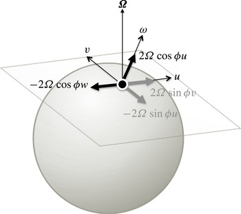
is the NT Coriolis parameter (see figure 1). Here
 $(u,v,w)$
are the Cartesian components of velocity in the tangent-plane basis. In spite of the fact that the vast majority of studies of the atmosphere and ocean dynamics at large scales is based on the TA, doubts with regard to this approximation are recurrent in the literature and were expressed, for example, by Bjerknes et al. (Reference Bjerknes, Bjerknes, Solberg and Bergeron1933), Phillips (Reference Phillips1966), Hendershott (Reference Hendershott, Warren and Wunsch1981), Müller (Reference Müller1989) and White & Bromley (Reference White and Bromley1995). The main reason for such doubts is that NT effects remain non-negligible in regions of weak stratification (Phillips Reference Phillips1968), or in the vicinity of the equator, where the factor
 $\cos {\it\phi}$
is large (White & Bromley Reference White and Bromley1995). More recent works have demonstrated that in some circumstances the NT component of the Coriolis force does have significant effects (see Gerkema et al. (Reference Gerkema, Zimmerman, Maas and Van Haren2008) for a complete review of NT effects in geophysical and astrophysical applications).
Components of the Coriolis force and flow velocity in the NT approximation: grey, traditional components associated with the vertical component of
 ${\it\bf\Omega}$
(proportional to
 $\sin {\it\phi}$
); black, NT components associated with the horizontal component of
 ${\it\bf\Omega}$
(proportional to
 $\cos {\it\phi}$
). Here
 ${\it\phi}$
is the latitude and
 $u,v,w$
are respectively the zonal, meridional and vertical components of velocity.

As already said, one can expect that the horizontal component of rotation should play a role at the equator, where the traditional Coriolis parameter
 $f=2{\it\Omega}\,\sin \,{\it\phi}$
vanishes while its NT counterpart
 $F=2{\it\Omega}\,\cos \,{\it\phi}$
takes the maximum value
 $2{\it\Omega}$
. Colin de Verdière & Schopp (Reference Colin de Verdière and Schopp1994) have shown that if the flow varies on a horizontal scale
 $L$
of the same order as or smaller than
 $\sqrt{Hr_{0}}$
, where
 $H$
is a vertical scale of motion and
 $r_{0}$
is the Earth’s radius, then equatorial dynamics must include the NT effects. This argument led Hua, Moore & Le Gentil (Reference Hua, Moore and Le Gentil1997) to take into account the NT component of the Coriolis force in a study of inertial equilibration of sub-thermocline equatorial ocean currents. Stewart & Dellar (Reference Stewart and Dellar2011a
,Reference Stewart and Dellar
b
) have shown that NT contributions to the angular momentum exchange modify the cross-equatorial water transport. Concerning the atmospheric flows, Hayashi & Itoh (Reference Hayashi and Itoh2012) showed the importance of the NT Coriolis terms for large-scale motions of the tropical atmosphere.
Yet, the NT part of the Coriolis force can influence the dynamics away from the equator as well. The NT effects were shown to modify dispersion, propagation and trapping properties of internal waves (Gerkema & Shrira Reference Gerkema and Shrira2005; Shrira & Townsend Reference Shrira, Townsend and Dritschel2010, Reference Shrira and Townsend2013; Winters, Bouruet-Aubertot & Gerkema Reference Winters, Bouruet-Aubertot and Gerkema2011; Colin de Verdière Reference Colin de Verdière2012; Reznik Reference Reznik2014). This fact is of importance because, besides their obvious role in wave propagation, dispersion and trapping, wave characteristics also condition the instabilities of background flows. As is well known, hydrodynamic instabilities can be interpreted by resonance and phase locking of the waves (counter-)propagating in the flow (e.g. Sakai Reference Sakai1989). So, by changing the wave properties, the NT effects can modify the instabilities of the flow. As the NT effects mostly affect short waves, they are presumably mostly relevant for ageostrophic instabilities. A special kind of ageostrophic instability is the inertial instability, due to the presence of trapped modes, and not due to phase-locked counter-propagating waves (Plougonven & Zeitlin Reference Plougonven and Zeitlin2005).
Inertial instability is of double interest in the context of NT corrections, as it is endemic at the equator. A number of analytical and numerical studies of linear and nonlinear stages of the inertial instability under the TA in homogeneous or linearly stratified fluids on the mid-latitude
 $f$
-plane (e.g. Kloosterziel, Carnevale & Orlandi Reference Kloosterziel, Carnevale and Orlandi2007a
; Kloosterziel, Orlandi & Carnevale Reference Kloosterziel, Orlandi and Carnevale2007b
; Griffiths Reference Griffiths2008; Plougonven & Zeitlin Reference Plougonven and Zeitlin2009; Bouchut, Ribstein & Zeitlin Reference Bouchut, Ribstein and Zeitlin2011; Ribstein, Plougonven & Zeitlin Reference Ribstein, Plougonven and Zeitlin2014a
) or equatorial
 ${\it\beta}$
-plane (Griffiths Reference Griffiths2003a
,Reference Griffiths
b
; Ribstein, Zeitlin & Tissier Reference Ribstein, Zeitlin and Tissier2014b
; Kloosterziel, Orlandi & Carnevale Reference Kloosterziel, Orlandi and Carnevale2015) exist in the literature. Some studies have already addressed the influence of the full Coriolis force upon the symmetric inertial instability, when the perturbations are invariant with respect to along-jet translations. Emanuel (Reference Emanuel1979) has discussed the inclusion of the meridional component of the Earth’s rotation while considering inertial instability of a shear flow, and concluded that the NT part of the Coriolis force should not affect the inertial stability problem in any significant way, except very close to the equator. Sun (Reference Sun1995) assumed the basic field velocity in traditional thermal wind balance without taking into account the fact that the NT terms modify the geostrophic balance. Using the energy–Casimir method, Fruman & Shepherd (Reference Fruman and Shepherd2008) derived a sufficient condition for linear stability with respect to zonally symmetric perturbations. Their results have confirmed that the marginal condition for inertial instability (determined by the sign of the potential vorticity) remains valid even when the TA is relaxed (Hua et al.
Reference Hua, Moore and Le Gentil1997). An analysis of the observed distribution of the angular momentum of sub-thermocline equatorially trapped ocean currents, whose vertically stacked structure is potentially linked to inertial instability (Hayashi, Shiotani & Gille Reference Hayashi, Shiotani and Gille1998), led Hua et al. (Reference Hua, Moore and Le Gentil1997) to take into account the complete Coriolis force in their numerical model, although the precise role and importance of the NT terms in the mechanism for the formation of deep equatorial jets is still to be clarified (Hua et al.
Reference Hua, Moore and Le Gentil1997; Gerkema et al.
Reference Gerkema, Zimmerman, Maas and Van Haren2008).
As was first pointed out by Dunkerton (Reference Dunkerton1983), besides the classical symmetric version of inertial instability, its asymmetric version also exists. It was studied under the TA in Bouchut et al. (Reference Bouchut, Ribstein and Zeitlin2011) and Ribstein et al. (Reference Ribstein, Plougonven and Zeitlin2014a ,Reference Ribstein, Zeitlin and Tissier b ) and was shown to be dominant in some flow regimes. Yet a general result for the inertial instability in a continuously stratified fluid states that symmetric instability is dominant at vertical wavenumber tending to infinity (Griffiths Reference Griffiths2008). No investigation of NT effects upon this kind of instability have been undertaken in the literature, to our knowledge.
Owing to the change in trapping properties of waves when relaxing the TA, one can expect that inertial instability in the equatorial region, where these effects are most pronounced, will be modified. As will be explained later, relaxing the TA on the equatorial
 ${\it\beta}$
-plane leads to specific technical problems (cf. also Maas Reference Maas2001; Gerkema & Shrira Reference Gerkema and Shrira2005) due to the non-separability of the linear stability problem even for a barotropic jet. This is why, as a first step to understanding the role of NT effects, we undertake in the present paper a study of ageostrophic instabilities of a barotropic jet on the mid-latitude
 $f$
-plane, where the non-separability problem can be circumvented. To keep continuity with previous studies, we choose the Bickley jet and, to focus on the domain of inertial instability, we limit ourselves to long-wave perturbations in the along-jet direction. Again, for the sake of continuity with previous works, we start our study with the two-layer rotating shallow-water model, and then compare the results with those in the full three-dimensional continuously stratified model. In the latter we also allow for NH effects and dissipation, necessary for the vertical scale selection (Griffiths Reference Griffiths2003b
), and investigate their role in conjunction with NT effects.
We will focus below on the stability of the Bickley jet, at some mid-latitude
 ${\it\phi}_{0}$
. We will use the
 $f$
-plane approximation, i.e. taking both traditional
 $f_{0}=2{\it\Omega}\sin {\it\phi}_{0}$
and non-traditional
 $F_{0}=2{\it\Omega}\cos {\it\phi}_{0}\approx f_{0}$
Coriolis parameters to be constant, neglecting their dependence on the meridional coordinate. The neglect of the
 ${\it\beta}$
term in the traditional Coriolis parameter is justified as
 ${\it\beta}L/f\approx L/r_{0}\ll 1$
, for jets with reasonable typical meridional extent
 $L$
. It is worth noting that if one wishes to consider meridional variation in the NT Coriolis parameter, one needs also to take into account vertical variation in the traditional Coriolis parameter in order to guarantee the conservation of absolute angular momentum (Dellar Reference Dellar2011; Tort & Dubos Reference Tort and Dubos2014).
The paper is organized as follows. In § 2, we formulate the linear stability problem for the mid-latitude Bickley jet in the two-layer shallow-water model on the NT
 $f$
-plane. The linear stability analysis is then performed with the help of the pseudo-spectral collocation method (Trefethen Reference Trefethen2000) and the unstable modes are identified and compared with their traditional counterparts for different values of the Burger and Rossby numbers and density/depth ratios. In § 3, we extend the linear stability analysis to a continuously stratified system in the Boussinesq approximation including the NT components of the Coriolis force. In the symmetric case and in the non-dissipative limit, we show that a reduction to a Sturm–Liouville problem is still possible relaxing the TA, with the help of a proper change of variables, and give analytical estimates of the growth rates, which serve later to benchmark numerical results. The NT unstable modes of both symmetric and asymmetric instabilities are identified and compared with those obtained with the TA for different background stratifications. The influence of dissipation and NH effects are quantified. Finally, a summary and discussion are given in § 4.
2. Linear stability analysis in the two-layer model
We consider in this section the two-layer rotating shallow-water equations on the NT
 $f$
-plane which were derived by Stewart & Dellar (Reference Stewart, Dellar, Fitt, Norbury, Ockendon and Wilson2010). The flow is a barotropic Bickley jet (in the sense of absence of vertical shear) evolving in mid-latitudes in the northern hemisphere, such that the traditional Coriolis parameter is positive
 $f>0$
and the NT Coriolis parameter is
 $F=O(\,f)$
. The model, the relevant parameters and the background flow configuration are presented in § 2.1. The linear stability problem is formulated in § 2.2, and linear stability analysis is performed for symmetric perturbations and weakly asymmetric perturbations in §§ 2.3 and 2.4, respectively.
2.1. Equations of motion and relevant parameters
The two-layer shallow-water equations with free upper surface and flat bottom on the NT
 $f$
-plane (Stewart & Dellar Reference Stewart, Dellar, Fitt, Norbury, Ockendon and Wilson2010) are
 $$\begin{eqnarray}\displaystyle & & \displaystyle \partial _{t}u_{1}+u_{1}\partial _{x}u_{1}+v_{1}\partial _{y}u_{1}-fv_{1}+g\partial _{x}(h_{1}+h_{2})\nonumber\\ \displaystyle & & \displaystyle \qquad -\,F\left(-v_{1}\partial _{y}h_{2}+\partial _{x}(h_{1}u_{1})+\partial _{x}(h_{2}u_{2})+\partial _{y}(h_{2}v_{2})+\frac{h_{1}\partial _{y}v_{1}}{2}\right)=0,\end{eqnarray}$$
 $$\begin{eqnarray}\displaystyle & \displaystyle \partial _{t}v_{1}+u_{1}\partial _{x}v_{1}+v_{1}\partial _{y}v_{1}+fu_{1}+g\partial _{y}(h_{1}+h_{2})-F\left(u_{1}\partial _{y}(h_{1}+h_{2})+\frac{h_{1}\partial _{y}u_{1}}{2}\right)=0, & \displaystyle\end{eqnarray}$$
 $$\begin{eqnarray}\displaystyle & \displaystyle \partial _{t}h_{1}+\partial _{x}(h_{1}u_{1})+\partial _{y}(h_{1}v_{1})=0, & \displaystyle\end{eqnarray}$$
 $$\begin{eqnarray}\displaystyle & \hspace{-18.00005pt}\displaystyle \partial _{t}u_{2}+u_{2}\partial _{x}u_{2}+v_{2}\partial _{y}u_{2}-fv_{2}+g\partial _{x}(h_{2}+rh_{1})-F\left(\partial _{x}(h_{2}u_{2})+r\partial _{x}(h_{1}u_{1})+\frac{h_{2}\partial _{y}v_{2}}{2}\right)=0,\hspace{-20.00003pt} & \displaystyle \nonumber\\ \displaystyle & & \displaystyle\end{eqnarray}$$
 $$\begin{eqnarray}\displaystyle & \displaystyle \partial _{t}v_{2}+u_{2}\partial _{x}v_{2}+v_{2}\partial _{y}v_{2}+fu_{2}+g\partial _{y}(h_{2}+rh_{1})-F\left(u_{2}\partial _{y}h_{2}+\frac{h_{2}\partial _{y}u_{2}}{2}+r\partial _{y}(h_{1}u_{1})\right)=0, & \displaystyle \nonumber\\ \displaystyle & & \displaystyle\end{eqnarray}$$
 $$\begin{eqnarray}\displaystyle & \displaystyle \partial _{t}h_{2}+\partial _{x}(h_{2}u_{2})+\partial _{y}(h_{2}v_{2})=0. & \displaystyle\end{eqnarray}$$
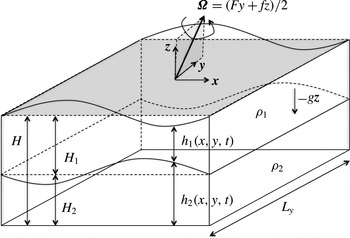
 $1~(2)$
refer to the top (bottom) layers (cf. figure 2). The density ratio is
 $r={\it\rho}_{1}/{\it\rho}_{2}<1$
, the height ratio is
 $d=H_{2}/H_{1}$
and the total height is
 $H=H_{1}+H_{2}$
.
Two-layer rotating shallow-water model on the NT
 $f$
-plane (northern hemisphere).

Under the TA with
 $F=0$
, the system with a typical velocity
 $U$
, horizontal scale
 $L$
and geopotential
 ${\it\phi}_{0}=gH$
is characterized by four dimensionless parameters: the Rossby number
 $\mathit{Ro}=U/(\,fL)$
, the barotropic Burger number
 $\mathit{Bu}={\it\phi}_{0}/(\,fL)^{2}$
,
 $r$
and
 $d$
. Close to the geostrophic balance,
 $$\begin{eqnarray}f\,\overline{v}_{i}=g\partial _{x}\overline{h}_{i},\quad f\,\overline{u}_{i}=-g\partial _{y}\overline{h}_{i},\quad i=1,2,\end{eqnarray}$$
which is valid at small
 $\mathit{Ro}$
, the non-dimensional deviations of the interface and of the free surface are of the order
 $\mathit{Ro}/\mathit{Bu}$
.
Relaxing the TA, the extra terms in (2.1)–(2.6) have a factor
 $F$
. The non-dimensionalization of (2.1)–(2.6) leads to the appearance of a new characteristic scale
 $FH$
. It corresponds to the typical scale of vertical variations of the planetary part of the absolute angular momentum (Dellar Reference Dellar2011; Tort et al.
Reference Tort, Dubos, Bouchut and Zeitlin2014; Tort & Dubos Reference Tort and Dubos2014)
 $\overline{u}-fy+Fh/2$
, in a homogeneous layer of height
 $h$
. The dimensionless parameter associated with this new scale is
 ${\it\delta}_{NT}=FH/(\,fL)$
and is of the order of the aspect ratio of the flow
 $H/L$
in mid-latitudes.
The NT two-layer shallow-water equations (2.1)–(2.6) inherit the conservation laws of the full compressible equations. In particular, there are two materially conserved potential vorticities (Stewart & Dellar Reference Stewart, Dellar, Fitt, Norbury, Ockendon and Wilson2010):
 $$\begin{eqnarray}\displaystyle & \displaystyle q_{1}=\frac{\partial _{x}v_{1}-\partial _{y}u_{1}+f-F\partial _{y}(h_{1}/2+h_{2})}{h_{1}}, & \displaystyle\end{eqnarray}$$
 $$\begin{eqnarray}\displaystyle & \displaystyle q_{2}=\frac{\partial _{x}v_{2}-\partial _{y}u_{2}+f-F\partial _{y}h_{2}/2}{h_{2}}. & \displaystyle\end{eqnarray}$$
Inertial instability requires that the product of the (traditional) Coriolis parameter and the absolute vorticity be negative. As NT
 $q_{i=\{1,2\}}$
differs by terms proportional to
 $F$
from the traditional potential vorticities for which
 $F=0$
in (2.8)–(2.9), the stability bounds may be altered.
We are considering a zonal barotropic Bickley jet with the velocity
 $$\begin{eqnarray}\overline{u}(y)=U\cosh ^{-2}(y/L),\quad \overline{v}(y)=0\end{eqnarray}$$
in both layers. Under the TA, in order to be an exact solution of the equations of motion, it is sufficient that such a velocity configuration satisfies the geostrophic balance conditions (2.7) which allow for immediate determination of the thicknesses
 $\overline{h}_{1,2}(y)$
from a given distribution of zonal velocity. The NT terms affect the geostrophic balance, and hence without the TA the layer thicknesses have to obey the following modified geostrophic balance equations:
 $$\begin{eqnarray}\displaystyle & \displaystyle \partial _{y}\overline{h}_{1}=-\frac{F\partial _{y}\overline{u}}{2(g-F\,\overline{u})(1-r)}(\overline{h}_{1}(2r-1)+\overline{h}_{2}), & \displaystyle\end{eqnarray}$$
 $$\begin{eqnarray}\displaystyle & \displaystyle \partial _{y}\overline{h}_{2}=\frac{1}{(g-F\,\overline{u})}\left(-f\,\overline{u}+\frac{F\partial _{y}\overline{u}}{2(1-r)}(r\overline{h}_{1}+\overline{h}_{2})\right). & \displaystyle\end{eqnarray}$$
 $MATLAB$
function ode45, in order to determine
 $\overline{h}_{1,2}(y)$
from
 $\overline{u}(y)$
.
Relevant flow parameters for the reference NT configuration.

The Earth parameters are
 $g=9.81$
m s
 $^{-2}$
,
 $r_{0}=6365$
km and
 ${\it\Omega}=2{\rm\pi}$
d
 $^{-1}$
. We present below the stability analysis for a reference configuration using
 $H\approx 20$
km,
 $L\approx 450$
km and
 $U\approx 80$
m s
 $^{-1}$
so that the typical
 $\mathit{Bu}$
is not too large allowing for the existence of the symmetric instability. (In any case, the dependence of the instability on
 $\mathit{Bu}$
will be carefully investigated below.) The latitude is
 ${\it\phi}_{0}=30^{\circ }$
for which the traditional Coriolis parameter is
 $f\approx 7\times 10^{-5}$
s
 $^{-1}$
while its meridional variation across the zonal jet is
 $2{\it\Omega}/r_{0}L\approx 9\times 10^{-6}$
s
 $^{-1}$
. As already said, the
 ${\it\beta}$
term of the traditional Coriolis parameter will be neglected, in accordance with the
 $f$
-plane approximation. The NT Coriolis parameter
 $F$
is zero under the TA, and is equal to
 $2{\it\Omega}\cos {\it\phi}_{0}$
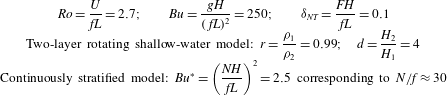
without the TA. The values of non-dimensional parameters for the reference configuration are given in table 1. Note that the jet has negative absolute vorticity, and thus is subject to inertial instability, for
 $\mathit{Ro}>3\sqrt{3}/4$
.
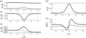
The numerical solution of (2.11) and (2.12) is plotted in figure 3 for values of the parameters corresponding to the reference configuration. The profile of the NT basic state is slightly modified in comparison with its traditional counterpart. While the height profile of the Bickley jet under the TA is a step-like hyperbolic tangent function, its NT counterpart has a bulge around
 $y=0$
. Differences in the potential vorticity (PV) profiles are indistinguishable. By analogy with the traditional inertial stability analysis, we can thus expect inertially unstable modes being trapped in the anticyclonic shear of the jet (negative potential vorticity region) as under the TA in the two-layer model (Bouchut et al.
Reference Bouchut, Ribstein and Zeitlin2011).
Background dimensionless jet profile (for the reference configuration, see table 1) as a function of
 $y/L$
. (a) Thickness
 $\overline{h}_{2}/H$
of layer 2 (dashed) and the total thickness
 $(\overline{h}_{1}+\overline{h}_{2})/H$
(solid). (c) Thickness of layer 1. (e) Thickness of layer 2, enlarged. (b) Velocity
 $\overline{u}(y)$
in both layers. (d) PV of layer 2 (dashed) and of layer 1 (solid). Grey, TA (
 ${\it\delta}_{NT}=0$
); black, NT (
 ${\it\delta}_{NT}=0.1$
). The difference between jet profile with and without the TA is perceptible only in the height profile. Owing to the smallness of the meridional gradient of height, the difference is indistinguishable in the PV profile.

2.2. Formulation of the linear stability problem
We add a small perturbation of the background jet,
 $u_{i}=\overline{u}(y)+u_{i}^{\prime }(x,y,t)$
,
 $v_{i}=v_{i}^{\prime }(x,y,t)$
and
 $h_{i}=\overline{h}(y)+h_{i}^{\prime }(x,y,t),i=1,2$
, linearize the system about the jet, and apply Fourier transformations in time and along-jet direction to the linearized equations (2.1)–(2.6). The solutions of the linearized system thus are sought in the form
 $(u_{i}^{\prime },v_{i}^{\prime },h_{i}^{\prime })=(\hat{u} _{i},\hat{v}_{i},{\hat{h}}_{i})\text{e}^{\text{i}(kx-{\it\omega}t)}+\text{c.c.}$
where
 $\text{c.c.}$
denotes the complex conjugate. We arrive in this way at the following eigenproblem:
 $$\begin{eqnarray}\displaystyle {\it\omega}\,\boldsymbol{X}=\unicode[STIX]{x1D648}\boldsymbol{\cdot }\boldsymbol{X},\quad \boldsymbol{X}=(\hat{u} _{1}(y),\text{i}\hat{v}_{1}(y),{\hat{h}}_{1}(y),\hat{u} _{2}(y),\text{i}\hat{v}_{2}(y),{\hat{h}}_{2}(y))^{\text{T}},\quad \unicode[STIX]{x1D648}=\left[\begin{array}{@{}cc@{}}\unicode[STIX]{x1D614}_{11} & \unicode[STIX]{x1D614}_{12}\\ \unicode[STIX]{x1D614}_{21} & \unicode[STIX]{x1D614}_{22}\end{array}\right]\!, & & \displaystyle \nonumber\\ \displaystyle & & \displaystyle\end{eqnarray}$$
where
 $$\begin{eqnarray}\displaystyle \unicode[STIX]{x1D614}_{11}=\left[\begin{array}{@{}ccc@{}}k(\overline{u}-F\,\overline{h}_{1}) & f-\mathscr{D}\overline{u}-F(\mathscr{D}\overline{h}_{2}-{\textstyle \frac{1}{2}}\overline{h}_{1}\mathscr{D}) & k(g-F\,\overline{u})\\ f-F(\mathscr{D}(\overline{h}_{1}+\overline{h}_{2})+{\textstyle \frac{1}{2}}\overline{h}_{1}\mathscr{D}) & k\overline{u} & (g-F\,\overline{u})\mathscr{D}-{\textstyle \frac{1}{2}}F\mathscr{D}\overline{u}\\ k\overline{h}_{1} & -(\overline{h}_{1}\mathscr{D}+\mathscr{D}\overline{h}_{1}) & k\overline{u}\end{array}\right]\!, & & \displaystyle \nonumber\\ \displaystyle & & \displaystyle\end{eqnarray}$$
 $$\begin{eqnarray}\displaystyle & \displaystyle \unicode[STIX]{x1D614}_{12}=\left[\begin{array}{@{}ccc@{}}-Fk\overline{h}_{2} & F(\mathscr{D}\overline{h}_{2}+\overline{h}_{2}\mathscr{D}) & k(g-F\,\overline{u})\\ 0 & 0 & (g-F\,\overline{u})\mathscr{D}\\ 0 & 0 & 0\end{array}\right]\!, & \displaystyle\end{eqnarray}$$
 $$\begin{eqnarray}\displaystyle & \displaystyle \unicode[STIX]{x1D614}_{21}=\left[\begin{array}{@{}ccc@{}}-Fkr\overline{h}_{1} & 0 & kr(g-F\,\overline{u})\\ -rF(\mathscr{D}\overline{h}_{1}+\overline{h}_{1}\mathscr{D}) & 0 & r((g-F\,\overline{u})\mathscr{D}-F\mathscr{D}\overline{u})\\ 0 & 0 & 0\end{array}\right]\!, & \displaystyle\end{eqnarray}$$
 $$\begin{eqnarray}\displaystyle & \displaystyle \unicode[STIX]{x1D614}_{22}=\left[\begin{array}{@{}ccc@{}}k(\overline{u}-F\,\overline{h}_{2}) & f-\mathscr{D}\overline{u}+{\textstyle \frac{1}{2}}F\,\overline{h}_{2}\mathscr{D} & k(g-F\,\overline{u})\\ f-F(\mathscr{D}\overline{h}_{2}+{\textstyle \frac{1}{2}}\overline{h}_{2}\mathscr{D}) & k\overline{u} & (g-F\,\overline{u})\mathscr{D}-{\textstyle \frac{1}{2}}F\mathscr{D}\overline{u}\\ k\overline{h}_{2} & -(\overline{h}_{2}\mathscr{D}+\mathscr{D}\overline{h}_{2}) & k\overline{u}\end{array}\right]\!. & \displaystyle\end{eqnarray}$$
 $[-5L,5L]$
defined by the Chebyshev collocation points (Boyd Reference Boyd2000; Trefethen Reference Trefethen2000)
 $y_{i}/(10L)=\cos (j{\rm\pi}/\mathscr{N}),j=\unicode[STIX]{x27E6}0,\mathscr{N}\unicode[STIX]{x27E7}$
, with
 $\mathscr{N}$
being the total number of collocation points, which are unevenly spaced in order to avoid the Runge phenomenon. Most of the points are thus located close to the domain boundaries
 $y=\pm L_{y}$
. As has already been mentioned, the modes trapped in the jet are important for inertial and related instabilities so a Kosloff/Tal-Ezer Arcsine mapping is used in order to uniformize the grid. Numerical convergence is typically achieved for
 $\mathscr{N}\geqslant 100$
. The Chebyshev differentiation matrix, denoted by
 $\mathscr{D}$
, is used for discrete differentiation.
The domain size
 $L_{y}$
has to be large enough to resolve the eigenmodes trapped in the negative part of PV, which has a characteristic length
 $L$
. Convergence of the results is achieved at
 $L_{y}\geqslant 10L$
. Taking
 $L_{y}=10L$
, we require the eigenmodes to vanish at
 $y=\pm 5L$
as we are mostly interested in trapped modes that decay far enough from the jet.
2.3. Results for the symmetric problem
We consider in this subsection the problem (2.13) with
 $k=0$
and thus we are looking for the classical symmetric inertial instability. Unstable modes, by definition, have
 $\text{Im}({\it\omega})>0$
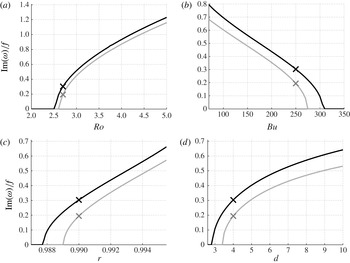
. The results for the growth rates
 $\text{Im}({\it\omega})$
of the unstable symmetric modes in the reference configuration are plotted as functions of
 $\mathit{Ro},~\mathit{Bu},r$
and
 $d$
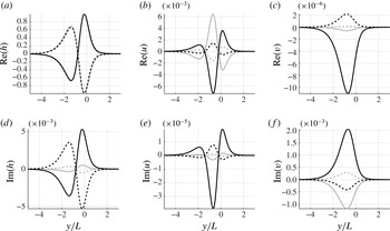
in figure 4. The meridional structure of the corresponding unstable modes is plotted in figure 5. The results can be summarized as follows.
At large enough
 $\mathit{Ro}$
, a single unstable mode is found. It is confined in the region of anticyclonic shear of the jet and is essentially baroclinic in the sense that the modes in the two layers have opposite signs. The nature of the instability and the form of the unstable modes are the same as with the TA, as for example the bell-shaped profile of the meridional velocity. As in the traditional case (Bouchut et al.
Reference Bouchut, Ribstein and Zeitlin2011), the growth rate
 $\text{Im}({\it\omega})$
increases with
 $\mathit{Ro},d,r$
and decreases with
 $\mathit{Bu}$
.
The NT growth rate is always higher. The NT terms thus have a destabilizing effect upon the symmetric inertial instability. There exists a parameter range where the jet is inertially unstable without the TA, while it is stable under the TA.
In the traditional symmetric problem, when
 $F=0$
, the linearized problem can be reduced to a pair of Schrödinger equations for
 $(u_{1},u_{2})$
. Using a decomposition of velocity in barotropic and baroclinic components, an integral estimate for
 ${\it\omega}^{2}$
can be obtained (Bouchut et al.
Reference Bouchut, Ribstein and Zeitlin2011) and the dependence on
 $\mathit{Ro},\mathit{Bu},r$
directly traced. The grey curves in figure 4 are consistent with this analysis, which serves as a benchmark for our numerical results. Such integral estimates are not available without the TA.
Dependence of the dimensionless growth rate
 $\text{Im}({\it\omega})/f$
(crosses indicate the reference configuration, see table 1) of the symmetric inertial instability on Rossby number
 $\mathit{Ro}$
(a),
 $\mathit{Bu}$
(b),
 $r$
(c) and
 $d$
(d). Grey, TA (
 ${\it\delta}_{NT}=0$
); black, NT (
 ${\it\delta}_{NT}=0.1$
).

Structure of the unstable mode of symmetric inertial instability, crosses in figure 6 (for the reference configuration, see table 1), as a function of
 $y/L$
. Dashed line, layer 2; solid line, layer 1. (a,d) Pressure, (b,e) zonal velocity, (c,f) meridional velocity. (a–c) Real part; (d–f) imaginary part. Grey, TA (
 ${\it\delta}_{NT}=0$
); black, NT (
 ${\it\delta}_{NT}=0.1$
).

2.4. Results for the asymmetric problem
Let us consider now the asymmetric problem (2.13) with
 $k\neq 0$
. The most important results of the stability analysis in this case are as follows.
In the ageostrophic regime, when
 $\mathit{Ro}\geqslant 1$
there are two leading instabilities of the jet: the barotropic and baroclinic inertial instabilities (Bouchut et al.
Reference Bouchut, Ribstein and Zeitlin2011). At sufficiently large
 $\mathit{Ro}$
, the growth rate of the baroclinic inertial instability is dominant for long waves, and has non-zero limit at
 $k\rightarrow 0$
. This is thus the asymmetric inertial instability, and the situation is the same as under the TA (Bouchut et al.
Reference Bouchut, Ribstein and Zeitlin2011). Analysis of the barotropic instability will not be presented.
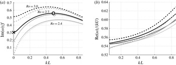
The NT growth rate of the asymmetric inertial instability is larger than that under the TA. The most unstable mode of the asymmetric inertial instability has smaller zonal wavenumber than with the TA. The difference between the growth rates in the two approximations is largest in the symmetric limit
 $(k=0)$
, where it can reach 30 %.
The most NT-unstable mode has larger phase speed than its traditional counterpart. The difference in phase speeds is not sensitive to the value of wavenumber in the long-wave sector.
Growth rates and phase speeds of the most unstable modes of the asymmetric inertial instability for the reference configuration at different
 $\mathit{Ro}$
are presented in figure 6. For
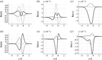
 $\mathit{Ro}=2.7$
(reference configuration) the meridional profiles of the three components of the most unstable mode are presented in figure 7. Note that they are practically identical to those for the symmetric inertial instability of figure 5, which allows us to conclude that the nature of the instability is the same, in spite of the presence of along-jet modulations.
Dimensionless growth rate
 $\text{Im}({\it\omega})/f$
and phase speed
 $\text{Re}({\it\omega})/(kU)$
of the most unstable mode of the barotropic Bickley jet in the two-layer model (baroclinic branch) as a function of dimensionless zonal wavenumber
 $kL$
for
 $\mathit{Ro}=2.4$
(dashed),
 $\mathit{Ro}=2.7$
(solid, reference configuration) and
 $\mathit{Ro}=3.0$
(dotted). (a) Dimensionless growth rate
 $\text{Im}({\it\omega})/f$
as a function of dimensionless wavenumber
 $kL$
. (b) Dimensionless phase velocity
 $\text{Re}({\it\omega})/(kU)$
as a function of dimensionless wavenumber
 $kL$
. Grey, TA (
 ${\it\delta}_{NT}=0$
); black, NT (
 ${\it\delta}_{NT}=0.1$
). Crosses and circles on (a) correspond to the symmetric instability and to the most unstable mode of asymmetric instability respectively within the reference configuration. The corresponding modes are plotted respectively in figures 5 and 7.

Meridional structure of the most unstable mode of the asymmetric inertial instability (for the reference configuration, see table 1), circles in figure 6. Dashed, layer 2; solid, layer 1. (a,d) Pressure, (b,e) zonal velocity, (c,f) meridional velocity. (a–c) Real part; (d–f) imaginary part. Grey, TA (
 ${\it\delta}_{NT}=0$
); black, NT (
 ${\it\delta}_{NT}=0.1$
).

2.5. Preliminary conclusions in the two-layer case
The inertial instability of the mid-latitude Bickley jet in the two-layer rotating shallow-water model is more vigorous without than with the TA, especially for the symmetric perturbations. Nevertheless, its nature remains the same, corresponding to essentially baroclinic inertial instability. The structure of the unstable modes is the same, reflecting trapping at the anticyclonic side of the jet.
3. Linear stability analysis in the continuously stratified model
We now present the results of the stability analysis of the barotropic jet in the case of continuous stratification, which is the standard framework for studying the inertial instability. We add viscosity and/or diffusivity, which are known to be essential for the vertical scale selection (Griffiths Reference Griffiths2003b ; Kloosterziel & Carnevale Reference Kloosterziel and Carnevale2008), and investigate the influence of NH effects. We will work with NT Boussinesq equations. As in § 2, we consider a barotropic Bickley jet evolving in mid-latitudes in the northern hemisphere. The model, parameters and the background flow configuration are presented in § 3.1. The linear stability problem is formulated in § 3.2. The results of linear stability analysis for perturbations with zero along-jet wavenumber are presented in § 3.3, and for non-zero but small along-jet wavenumbers in § 3.4.
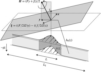
Barotropic jet in the Boussinesq model on the NT
 $f$
-plane (northern hemisphere). The vector
 ${\bf\xi}$
is perpendicular to the total rotation vector
 ${\it\bf\Omega}$
. The barotropic velocity profile
 $\overline{u}({\it\xi})$
is a function of
 ${\it\xi}$
, the new coordinate corresponding to
 ${\bf\xi}$
.

3.1. Equations of motion and relevant parameters
In the atmospheric context, the NT primitive equations on the
 $f$
-plane in the Boussinesq approximation (Phillips Reference Phillips1966), including vertical (turbulent) viscosity and diffusivity, are
 $$\begin{eqnarray}\displaystyle & \displaystyle (\partial _{t}+u\partial _{x}+v\partial _{y}+w\partial _{z})u-fv+Fw+\partial _{x}{\it\Phi}-{\it\nu}\partial _{zz}u=0, & \displaystyle\end{eqnarray}$$
 $$\begin{eqnarray}\displaystyle & \displaystyle (\partial _{t}+u\partial _{x}+v\partial _{y}+w\partial _{z})v+fu+\partial _{y}{\it\Phi}-{\it\nu}\partial _{zz}v=0, & \displaystyle\end{eqnarray}$$
 $$\begin{eqnarray}\displaystyle & \displaystyle (\partial _{t}+u\partial _{x}+v\partial _{y}+w\partial _{z}){\it\theta}-{\it\kappa}\partial _{zz}{\it\theta}=0, & \displaystyle\end{eqnarray}$$
 $$\begin{eqnarray}\displaystyle & \displaystyle {\it\delta}_{NH}(\partial _{t}+u\partial _{x}+v\partial _{y}+w\partial _{z})w+\partial _{z}{\it\Phi}+b-Fu-{\it\delta}_{NH}{\it\nu}\partial _{zz}w=0, & \displaystyle\end{eqnarray}$$
 $$\begin{eqnarray}\displaystyle & \displaystyle \partial _{x}u+\partial _{y}v+\partial _{z}w=0, & \displaystyle\end{eqnarray}$$
 ${\it\nu}$
and
 ${\it\kappa}$
are, respectively, vertical (turbulent) viscosity and (turbulent) diffusivity (as usual, we anticipate that the smallest scales occur in the vertical direction),
 ${\it\Phi}$
is geopotential and
 ${\it\theta}$
is potential temperature. The buoyancy is defined as
 $b=-g{\it\theta}/{\it\theta}_{r}$
, where
 ${\it\theta}_{r}$
is a reference potential temperature. The vertical coordinate
 $z$
is a pseudo-height introduced by Hoskins & Bretherton (Reference Hoskins and Bretherton1972), differing slightly from the geometric height for a shallow fluid layer;
 $u,v$
and
 $w$
are, respectively, zonal (
 $x$
direction), meridional (
 $y$
direction) and vertical (
 $z$
direction) components of velocity (see figure 8). In the vertical momentum equation (3.4), we include an NH switch
 ${\it\delta}_{NH}$
. Setting
 ${\it\delta}_{NH}=1$
gives the full equation set while setting
 ${\it\delta}_{NH}=0$
approximates the vertical momentum equation by the (quasi-)hydrostatic balance (the NT terms affect the hydrostatic balance, which will be therefore called quasi-hydrostatic).
For simplicity, we consider a rest state with a stable linear stratification
 ${\it\theta}_{0}(z)$
and Brunt–Väisälä frequency
 $N=\sqrt{g\partial _{z}{\it\theta}_{0}/{\it\theta}_{r}}=\text{const}$
. The system is characterized by a typical horizontal velocity
 $U$
, a typical horizontal length
 $L$
, geopotential
 ${\it\phi}_{0}=gH$
, frequency
 $N$
, and a new NT scale
 $FH$
(vertical variation of planetary velocity). The dimensionless parameters are then the Rossby number
 $\mathit{Ro}=U/(\,fL)$
, the barotropic Burger number
 $\mathit{Bu}={\it\phi}_{0}/(\,fL)^{2}$
, the baroclinic Burger number
 $\mathit{Bu}^{\ast }=(NH/(\,fL))^{2}$
, and the NT parameter
 ${\it\delta}_{NH}=FH/(\,fL)$
. For the sake of comparison with the two-layer shallow-water system, the same reference configuration as defined in § 2 and table 1 is used, also at
 $30^{\circ }$
north. To make a link with the two-layer shallow-water reference configuration considered previously, the density ratio
 $r=0.99$
would correspond to
 $N=\sqrt{g(1-r)/H}=2\times 10^{-3}$
s
 $^{-1}$
.
We consider a barotropic balanced jet
 $({\it\Phi}_{ref}(y,z),u_{ref}(y,z))$
with the background vertical structure defined by
 $({\it\theta}_{0}(z),{\it\Phi}_{0}(y,z))$
. The jet is then a solution of the equations
 $$\begin{eqnarray}\displaystyle & \displaystyle fu_{ref}+\partial _{y}{\it\Phi}_{ref}=0, & \displaystyle\end{eqnarray}$$
 $$\begin{eqnarray}\displaystyle & \displaystyle \partial _{z}{\it\Phi}_{ref}+b_{0}-Fu_{ref}=0, & \displaystyle\end{eqnarray}$$
 $b_{0}=-g{\it\theta}_{0}/{\it\theta}_{r}$
. By cross-differentiation of (3.6) and (3.7) we get
 $$\begin{eqnarray}\displaystyle (\,f\partial _{z}+F\partial _{y})u_{ref}=0, & & \displaystyle\end{eqnarray}$$
as
 $\partial _{y}b_{0}=0$
. This means that the velocity of the barotropic jet is a function of both meridional and vertical coordinates, which in turn means that linearization about such a profile will give a non-separable problem. However, it is clear from (3.8) that the jet velocity is a function of
 ${\it\xi}=y-(F/f)z$
only:
 $u_{ref}(y,z)=\overline{u}({\it\xi})$
, which suggests a change of variable
 $y\rightarrow {\it\xi}$
. Denoting
 ${\it\Phi}_{ref}(y,z)=\overline{{\it\Phi}}({\it\xi})+{\it\Phi}_{0}(z)$
we have
 $\partial _{y}{\it\Phi}_{ref}=\partial _{{\it\xi}}\overline{{\it\Phi}}$
,
 $\partial _{z}{\it\Phi}_{ref}=\partial _{z}{\it\Phi}_{0}(z)-F/f\partial _{{\it\xi}}\overline{{\it\Phi}}$
, and using (3.6)–(3.7) we get
 $$\begin{eqnarray}\displaystyle & \displaystyle f\,\overline{u}+\partial _{{\it\xi}}\overline{{\it\Phi}}=0, & \displaystyle\end{eqnarray}$$
 $$\begin{eqnarray}\displaystyle & \displaystyle \partial _{z}{\it\Phi}_{0}+b_{0}=0, & \displaystyle\end{eqnarray}$$
 $({\it\xi},z)$
. By the change of independent variables
 $(x,y,z)\rightarrow (x,{\it\xi},z)$
, we thus obtain that the barotropic balanced Bickley jet, which is an exact solution of (3.1)–(3.5), has the form
 $$\begin{eqnarray}\left(\overline{{\it\Phi}}({\it\xi})={\it\phi}_{0}(1-\tanh ({\it\xi}/L)),\overline{u}({\it\xi})=U\cosh ^{-2}({\it\xi}/L)\right)\end{eqnarray}$$
and is defined entirely in terms of the ‘tilted’ meridional coordinate
 ${\it\xi}$
. The geometry of the problem modified by the change of variable
 $(x,y,z)\rightarrow (x,{\it\xi},z)$
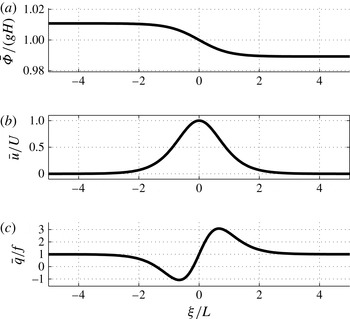
is sketched in figure 8. The profile of the background jet as a function of
 ${\it\xi}/L$
is plotted in figure 9 within the reference configuration. The mean absolute vorticity becomes
 $\overline{q}=f-\partial _{{\it\xi}}\overline{u}$
.
Background dimensionless jet profile as a function of
 ${\it\xi}/L$
(for the reference configuration, see table 1). (a) Geopotential
 $\overline{{\it\Phi}}$
, (b) zonal velocity
 $\overline{u}$
, (c) PV
 $\overline{q}$
. As a function of
 ${\it\xi}$
instead of meridional coordinate
 $y$
, the NT profile is identical to its traditional counterpart. The traditional profile is recovered at
 ${\it\xi}=y$
corresponding to
 $F=0$
.

3.2. Formulation of the linear stability problem
We consider small perturbations of the basic state,
 ${\it\Phi}={\it\Phi}_{0}(z)+\overline{{\it\Phi}}({\it\xi})+{\it\Phi}^{\prime }(x,{\it\xi},z)$
,
 $b=b_{0}(z)+b^{\prime }(x,{\it\xi},z)$
,
 $u=\overline{u}({\it\xi})+u^{\prime }(x,{\it\xi},z)$
,
 $v=v^{\prime }(x,{\it\xi},z)$
,
 $w=w^{\prime }(x,{\it\xi},z)$
and linearize the equations (3.1)–(3.5) about the jet. All variables are expressed in the new coordinate system
 $(x,{\it\xi},z)$
, using the relationships
 $$\begin{eqnarray}\displaystyle \partial _{y}G=\partial _{{\it\xi}}\tilde{G}\quad \text{and}\quad \partial _{z}G=\partial _{z}\tilde{G}-F/f\partial _{{\it\xi}}\tilde{G}, & & \displaystyle\end{eqnarray}$$
for any function
 $G(x,y,z)=\tilde{G}(x,{\it\xi},z)$
. Tildes in such expressions will be omitted from now on. We get in this way the following system:
 $$\begin{eqnarray}\displaystyle & \displaystyle \left(\partial _{t}+\overline{u}\partial _{x}-{\it\nu}\left(\partial _{z}-\frac{F}{f}\partial _{{\it\xi}}\right)^{2}\right)u^{\prime }-\overline{q}\hat{v}^{\prime }+\partial _{x}{\it\Phi}^{\prime }=0, & \displaystyle\end{eqnarray}$$
 $$\begin{eqnarray}\displaystyle & \displaystyle \left(\partial _{t}+\overline{u}\partial _{x}-{\it\nu}\left(\partial _{z}-\frac{F}{f}\partial _{{\it\xi}}\right)^{2}\right)\left(\hat{v}^{\prime }+\frac{F}{f}w^{\prime }\right)+fu^{\prime }+\partial _{{\it\xi}}{\it\Phi}^{\prime }=0, & \displaystyle\end{eqnarray}$$
 $$\begin{eqnarray}\displaystyle & \displaystyle \left(\partial _{t}+\overline{u}\partial _{x}-{\it\kappa}\left(\partial _{z}-\frac{F}{f}\partial _{{\it\xi}}\right)^{2}\right)b^{\prime }-w^{\prime }N^{2}=0, & \displaystyle\end{eqnarray}$$
 $$\begin{eqnarray}\displaystyle & \displaystyle {\it\delta}_{NH}\left(\partial _{t}+\overline{u}\partial _{x}-{\it\nu}\left(\partial _{z}-\frac{F}{f}\partial _{{\it\xi}}\right)^{2}\right)w^{\prime }+\left(\partial _{z}-\frac{F}{f}\partial _{{\it\xi}}\right){\it\Phi}^{\prime }+b^{\prime }-Fu^{\prime }=0, & \displaystyle\end{eqnarray}$$
 $$\begin{eqnarray}\displaystyle & \displaystyle \partial _{x}u^{\prime }+\partial _{{\it\xi}}\hat{v}^{\prime }+\partial _{z}w^{\prime }=0, & \displaystyle\end{eqnarray}$$
 $\hat{v}^{\prime }=v^{\prime }-(F/f)w^{\prime }$
. Solutions of this system are sought in the form:
 $$\begin{eqnarray}({\it\Phi}^{\prime },b^{\prime },u^{\prime },\hat{v}^{\prime },w^{\prime })=({\it\Phi}({\it\xi}),b({\it\xi}),u({\it\xi}),v({\it\xi}),w({\it\xi}))\text{e}^{\text{i}(kx+mz-{\it\omega}t)}+\text{c.c.}\end{eqnarray}$$
Let us recall that under the TA (when
 ${\it\xi}\equiv y$
), by use of Fourier transform (3.18) the eigenproblem (3.13)–(3.17) can be reduced to the
 $3\times 3$
matrix form:
 ${\it\omega}\,\unicode[STIX]{x1D64B}\boldsymbol{\cdot }({\it\Phi},u,v)^{\text{T}}=\unicode[STIX]{x1D648}\boldsymbol{\cdot }({\it\Phi},u,v)^{\text{T}}$
, where
 $\unicode[STIX]{x1D64B}$
is the identity matrix when
 ${\it\delta}_{NH}=0$
(see Ribstein et al.
Reference Ribstein, Zeitlin and Tissier2014b
) and some non-diagonal matrix when
 ${\it\delta}_{NH}=1$
. When relaxing the TA, but keeping the hydrostatic approximation, the eigenproblem can still be reduced to the same form, but NT and dissipative terms lead to the appearance of non-diagonal terms in the matrix
 $\unicode[STIX]{x1D64B}$
in this case. If the hydrostatic approximation is relaxed, the mathematical structure of the problem is modified, and we choose to treat the NT NH stability problem in terms of four variables
 $(u,v,b,{\it\Phi})$
, by eliminating
 $w$
from the continuity equation (3.17). For this reason, as in Ribstein et al. (Reference Ribstein, Zeitlin and Tissier2014b
), we have to exclude from the analysis the perturbation associated with a vertical wavenumber
 $m=0$
(a purely barotropic mode).
3.2.1. Linear stability problem in the hydrostatic limit
We consider here the equations (3.13)–(3.17) with
 ${\it\delta}_{NH}=0$
. Using Fourier transform (3.18) we get
 $$\begin{eqnarray}\displaystyle & \displaystyle \left(-{\it\omega}+k\overline{u}+\text{i}{\it\nu}\left(\text{i}m-\frac{F}{f}\partial _{{\it\xi}}\right)^{2}\right)u+\overline{q}\text{i}v+k{\it\Phi}=0, & \displaystyle\end{eqnarray}$$
 $$\begin{eqnarray}\displaystyle & \displaystyle \left(-{\it\omega}+k\overline{u}+\text{i}{\it\nu}\left(\text{i}m-\frac{F}{f}\partial _{{\it\xi}}\right)^{2}\right)\left(\text{i}v+\frac{\text{i}F}{f}\frac{\partial _{{\it\xi}}\text{i}v-ku}{m}\right)+fu+\partial _{{\it\xi}}{\it\Phi}=0, & \displaystyle\end{eqnarray}$$
 $$\begin{eqnarray}\displaystyle & \displaystyle \left(-{\it\omega}+k\overline{u}+\text{i}{\it\kappa}\left(\text{i}m-\frac{F}{f}\partial _{{\it\xi}}\right)^{2}\right)b+\text{i}N^{2}\frac{\partial _{{\it\xi}}\text{i}v-ku}{m}=0, & \displaystyle\end{eqnarray}$$
 $b=(F/f\partial _{{\it\xi}}-\text{i}m){\it\Phi}+Fu$
and
 $\text{i}w=\text{i}(\partial _{{\it\xi}}\text{i}v-ku)/m$
for
 $m\neq 0$
. The pure barotropic mode with
 $m=0$
needs special treatment. As already said above in § 3.2, we will exclude this mode in what follows, considering only the perturbations associated with
 $k\geqslant 0$
and
 $m>0$
. Substituting
 $b$
and
 $\text{i}w$
in (3.19)–(3.21), we get
 $$\begin{eqnarray}\displaystyle & \displaystyle \mathscr{G}({\it\nu})u+\overline{q}\text{i}v+k{\it\Phi}={\it\omega}u, & \displaystyle\end{eqnarray}$$
 $$\begin{eqnarray}\displaystyle & \displaystyle \left(\,f-\frac{\text{i}Fk}{fm}\mathscr{G}({\it\nu})\right)u+\mathscr{G}({\it\nu})\text{i}v+\mathscr{D}{\it\Phi}={\it\omega}\left(-\frac{\text{i}Fk}{fm}u+\mathscr{F}\text{i}v\right), & \displaystyle\end{eqnarray}$$
 $$\begin{eqnarray}\displaystyle & \displaystyle \left(\mathscr{G}({\it\kappa})\frac{\text{i}F}{m}+\frac{N^{2}}{m^{2}}k\right)u-\frac{N^{2}}{m^{2}}\partial _{{\it\xi}}\text{i}v+\mathscr{G}({\it\kappa}){\it\Phi}={\it\omega}\left(\frac{\text{i}F}{m}u+\mathscr{F}{\it\Phi}\right), & \displaystyle\end{eqnarray}$$
 $\mathscr{D}=\partial _{{\it\xi}}$
,
 $\mathscr{F}=(1+(\text{i}F/mf)\mathscr{D})$
and
 $\mathscr{G}({\it\nu})=k\overline{u}-\text{i}{\it\nu}m^{2}\mathscr{F}^{2}$
. The eigenproblem then is reduced to
 $$\begin{eqnarray}\displaystyle {\it\omega}\,\unicode[STIX]{x1D64B}\boldsymbol{\cdot }\boldsymbol{X}=\unicode[STIX]{x1D648}\boldsymbol{\cdot }\boldsymbol{X},\quad \boldsymbol{X}=(u,\text{i}v,{\it\Phi})^{\text{T}}, & & \displaystyle\end{eqnarray}$$
with
 $$\begin{eqnarray}\unicode[STIX]{x1D64B}=\left[\begin{array}{@{}ccc@{}}1 & 0 & 0\\ \displaystyle -\frac{\text{i}Fk}{fm} & \mathscr{F} & 0\\ \displaystyle \frac{\text{i}F}{m} & 0 & \mathscr{F}\end{array}\right],\quad \unicode[STIX]{x1D648}=\left[\begin{array}{@{}ccc@{}}\mathscr{G}({\it\nu}) & \overline{q} & k\\ f-\displaystyle \frac{\text{i}Fk}{fm}\mathscr{G}({\it\nu}) & \mathscr{G}({\it\nu}) & \mathscr{D}\\ \displaystyle \frac{N^{2}k}{m^{2}}+\frac{\text{i}F}{m}\mathscr{G}({\it\kappa}) & \displaystyle -\frac{N^{2}}{m^{2}}\mathscr{D} & \mathscr{G}({\it\kappa})\end{array}\right].\end{eqnarray}$$
In the traditional limit, when
 $F\rightarrow 0$
,
 $\mathscr{F}=\unicode[STIX]{x1D644}$
,
 $\mathscr{D}=\partial _{y}$
and
 $\mathscr{G}({\it\nu})=k\overline{u}-\text{i}{\it\nu}m^{2}$
, the matrix system of Ribstein et al. (Reference Ribstein, Zeitlin and Tissier2014b
) is recovered.
3.2.2. Non-hydrostatic system
As already said in § 3.2, we will treat the NH problem in terms of
 $(u,v,b,{\it\Phi})$
eliminating only
 $w$
with the help of the continuity equation. We get
 $$\begin{eqnarray}\displaystyle {\it\omega}\,\unicode[STIX]{x1D64B}\boldsymbol{\cdot }\boldsymbol{X}=\unicode[STIX]{x1D648}\boldsymbol{\cdot }\boldsymbol{X},\quad \boldsymbol{X}=(u,\text{i}v,b,{\it\Phi})^{\text{T}}, & & \displaystyle\end{eqnarray}$$
where
 $$\begin{eqnarray}\displaystyle & \displaystyle \unicode[STIX]{x1D64B}=\left[\begin{array}{@{}cccc@{}}1 & 0 & 0 & 0\\ \displaystyle -\frac{\text{i}Fk}{fm} & \mathscr{F} & 0 & 0\\ 0 & 0 & \displaystyle \frac{1}{m} & 0\\ -{\it\delta}_{NH}\displaystyle \frac{\text{i}k}{m} & {\it\delta}_{NH}\displaystyle \frac{\text{i}}{m}\mathscr{D} & 0 & 0\end{array}\right], & \displaystyle\end{eqnarray}$$
 $$\begin{eqnarray}\displaystyle & \displaystyle \unicode[STIX]{x1D648}=\left[\begin{array}{@{}cccc@{}}\mathscr{G}({\it\nu}) & \overline{q} & 0 & k\\ \displaystyle f-\frac{\text{i}Fk}{fm}\mathscr{G}({\it\nu}) & \mathscr{G}({\it\nu})\mathscr{F} & 0 & \mathscr{D}\\ \displaystyle -\frac{\text{i}N^{2}k}{m^{2}} & \displaystyle \frac{\text{i}N^{2}}{m^{2}}\mathscr{D} & \displaystyle \frac{1}{m}\mathscr{G}({\it\kappa}) & 0\\ -\!\left({\it\delta}_{NH}\displaystyle \frac{\text{i}k\mathscr{G}({\it\nu})}{m}+F\right) & {\it\delta}_{NH}\displaystyle \frac{\text{i}\mathscr{G}({\it\nu})}{m}\mathscr{D} & 1 & \text{i}m\mathscr{F}\end{array}\right]. & \displaystyle\end{eqnarray}$$
3.3. Results of the linear stability analysis for the symmetric problem
We will consider in this section the symmetric variant of (3.27) when
 $k=0$
. We first provide some integral estimates for the eigenvalues
 ${\it\omega}$
in § 3.3.1, and then present results of numerical analysis of the linear stability in § 3.3.2.
3.3.1. Analytical results in particular cases: difference between the growth rates with and without the TA
After some algebra, the non-dissipative (
 ${\it\nu}={\it\kappa}=0$
) symmetric (
 $k=0$
) problem (3.27) can be reduced to a single equation for
 $v$
:
 $$\begin{eqnarray}\displaystyle {\it\omega}^{2}\left(\left(\frac{F}{fm}\partial _{{\it\xi}}-\text{i}\right)^{2}+\frac{{\it\delta}_{NH}}{m^{2}}\partial _{{\it\xi}{\it\xi}}\right)v=\left(\frac{N^{2}}{m^{2}}\partial _{{\it\xi}{\it\xi}}-f\,\overline{q}\right)v, & & \displaystyle\end{eqnarray}$$
which allows us to obtain analytical estimates in some particular cases.
(i) Hydrostatic limit
 ${\it\delta}_{NH}=0$
. In this case (3.30) becomes
 $$\begin{eqnarray}\displaystyle {\it\omega}^{2}\left(\frac{F}{fm}\partial _{{\it\xi}}-\text{i}\right)^{2}v=\left(\frac{N^{2}}{m^{2}}\partial _{{\it\xi}{\it\xi}}-f\,\overline{q}\right)v & & \displaystyle\end{eqnarray}$$
and represents a modified Sturm–Liouville problem, where operator
 $(F\partial _{{\it\xi}}/(\,fm)-\text{i})^{2}$
is a complex self-adjoint operator. Hence
 ${\it\omega}^{2}$
is real, although the eigenfunction
 $v$
is complex. We use the polar decomposition of
 $v$
:
 $v=|v|\exp (\text{i}{\it\varphi})$
. Substituting this expression into (3.31) and separating the real and imaginary parts we obtain
 $$\begin{eqnarray}\displaystyle & \displaystyle \left(\left(\frac{{\it\omega}F}{mf}\right)^{2}-\left(\frac{N}{m}\right)^{2}\right)(\partial _{{\it\xi}{\it\xi}}|v|-|v|(\partial _{{\it\xi}}{\it\varphi})^{2})+\left(2{\it\omega}^{2}\frac{F}{mf}\partial _{{\it\xi}}{\it\varphi}-{\it\omega}^{2}+f\,\overline{q}\right)|v|=0, & \displaystyle\end{eqnarray}$$
 $$\begin{eqnarray}\displaystyle & \displaystyle \partial _{{\it\xi}}\left(\left(\left(\frac{{\it\omega}F}{mf}\right)^{2}-\left(\frac{N}{m}\right)^{2}\right)(|v|^{2}\partial _{{\it\xi}}{\it\varphi})-{\it\omega}^{2}\frac{F}{mf}|v|^{2}\right)=0. & \displaystyle\end{eqnarray}$$
 ${\it\xi}$
and using the decay boundary conditions for
 $|v|$
, relevant for the trapped modes of inertial instability, we get
 $$\begin{eqnarray}\left(\left({\it\omega}\frac{F}{f}\right)^{2}-N^{2}\right)\partial _{{\it\xi}}{\it\varphi}={\it\omega}^{2}m\frac{F}{f}.\end{eqnarray}$$
Substituting the integration result (3.34) in (3.32) yields
 $$\begin{eqnarray}\displaystyle \frac{1}{m^{2}}\left(\left(\frac{F}{f}{\it\omega}\right)^{2}-N^{2}\right)^{2}\partial _{{\it\xi}{\it\xi}}|v|+N^{2}{\it\omega}^{2}|v|+\left(\left(\frac{F}{f}{\it\omega}\right)^{2}-N^{2}\right)f\,\overline{q}|v|=0. & & \displaystyle\end{eqnarray}$$
The non-dimensional version of this equation, where the scales
 $L$
,
 $H$
,
 $U$
and
 $f^{-1}$
are used, respectively, for horizontal and vertical dimensions, velocities and time, is
 $$\begin{eqnarray}\displaystyle & & \displaystyle \left(\frac{1}{\mathit{Bu}^{\ast }}\left(\frac{{\it\delta}_{NT}^{2}}{m}\right)^{2}{\it\omega}^{4}-2\left(\frac{{\it\delta}_{NT}}{m}\right)^{2}{\it\omega}^{2}+\frac{\mathit{Bu}^{\ast }}{m^{2}}\right)\partial _{{\it\xi}{\it\xi}}|v|\nonumber\\ \displaystyle & & \displaystyle \qquad +\,{\it\omega}^{2}|v|+\left(\frac{{\it\delta}_{NT}^{2}}{\mathit{Bu}^{\ast }}{\it\omega}^{2}-1\right)(1-\mathit{Ro}\partial _{y}\overline{u})|v|=0.\end{eqnarray}$$
The NT terms in (3.36) are multiplied by the dimensionless parameters
 $$\begin{eqnarray}({\it\delta}_{NT}^{2}/m)^{2}/\mathit{Bu}^{\ast },\quad ({\it\delta}_{NT}/m)^{2}\quad \text{and}\quad {\it\delta}_{NT}^{2}/\mathit{Bu}^{\ast }.\end{eqnarray}$$
For large
 $\mathit{Bu}^{\ast }$
(relevant for strong stratification
 $N\gtrsim f$
) and small
 ${\it\delta}_{NT}$
(relevant for mid-latitude dynamics where
 ${\it\delta}_{NT}\approx H/L$
), we then deduce that the NT terms have small influence on the growth rate of the symmetric instability. We may then neglect the term with the factor
 ${\it\omega}^{4}$
which is at least an order of magnitude smaller than the other NT terms in (3.35). In this case (3.35) becomes
 $$\begin{eqnarray}\displaystyle \left(-2\left(\frac{{\it\omega}F}{fm}\right)^{2}+\left(\frac{N}{m}\right)^{2}\right)\partial _{{\it\xi}{\it\xi}}|v|+{\it\omega}^{2}|v|+\left(\left(\frac{{\it\omega}F}{Nf}\right)^{2}-1\right)f\,\overline{q}|v|=0. & & \displaystyle\end{eqnarray}$$
Considering trapped modes, multiplying (3.38) by
 $|v|$
and integrating in
 ${\it\xi}$
from
 ${\it\xi}=-\infty$
to
 ${\it\xi}=+\infty$
, we get the following integral estimate for
 ${\it\omega}^{2}$
:
 $$\begin{eqnarray}{\it\omega}^{2}=\frac{\displaystyle \int _{-\infty }^{+\infty }\text{d}{\it\xi}\left(\left(\frac{N}{m}\right)^{2}|\partial _{{\it\xi}}v|^{2}+f\,\overline{q}|v|^{2}\right)}{\displaystyle \int _{-\infty }^{+\infty }\text{d}{\it\xi}\left(2\left(\frac{F}{fm}\right)^{2}|\partial _{{\it\xi}}v|^{2}+\left(1+\left(\frac{F}{Nf}\right)^{2}f\,\overline{q}\right)|v|^{2}\right)}.\end{eqnarray}$$
For large
 $m$
, we may neglect the terms containing
 $1/m^{2}$
in this equation. Denoting by
 ${\it\omega}_{NT}$
the solution of equation (3.39) and recalling that in the same approximation the TA result is
 $$\begin{eqnarray}\displaystyle {\it\omega}_{trad}^{2}\approx \frac{\displaystyle \int _{-\infty }^{+\infty }\text{d}{\it\xi}\,f\,\overline{q}|v|^{2}}{\displaystyle \int _{-\infty }^{+\infty }\text{d}{\it\xi}\,|v|^{2}}, & & \displaystyle\end{eqnarray}$$
we get
 $$\begin{eqnarray}\displaystyle \frac{{\it\omega}_{NT}^{2}-{\it\omega}_{trad}^{2}}{{\it\omega}_{NT}^{2}}\approx -\left(\frac{F}{Nf}\right)^{2}{\it\omega}_{trad}^{2}. & & \displaystyle\end{eqnarray}$$
We conclude that, if the instability is present under the TA, i.e.
 ${\it\omega}_{trad}^{2}<0$
, then its growth rate is lower than for its NT counterpart:
 $(\text{Im}({\it\omega}_{trad})/\text{Im}({\it\omega}_{NT}))^{2}\approx 1-(F/(\,fN))^{2}\,\text{Im}({\it\omega}_{trad})^{2}<1$
. Estimates (3.39) and (3.41) will be used to check the numerical results for
 ${\it\omega}_{NT}$
. The difference between traditional and NT growth rates of the symmetric inertial instability increases when stratification decreases, but remains non-neutral:
 $N\gtrsim f$
.
(ii) Neutral stratification
 $N^{2}=0$
. With
 $N^{2}=0$
, (3.30) becomes
 $$\begin{eqnarray}\displaystyle {\it\omega}^{2}\left(\left(\frac{F}{fm}\partial _{{\it\xi}}v-\text{i}\right)^{2}+\frac{{\it\delta}_{NH}}{m^{2}}\partial _{{\it\xi}{\it\xi}}\right)v=-f\,\overline{q}v. & & \displaystyle\end{eqnarray}$$
Under hydrostatic and traditional approximations,
 ${\it\omega}_{trad}^{2}v=f\,\overline{q}v$
. Hence
 $v\equiv 0$
, and no information on
 ${\it\omega}_{trad}$
can be obtained. We thus have to come back to the full eigenproblem in terms of all variables and analyse it at
 $v=0$
. Such analysis in the symmetric non-dissipative limit shows that the eigenvector represents a zero-mode stationary solution (the thermal wind) with zero eigenvalue. Therefore, the flow is stable in this case. This means that inertial instability is impossible under the TA under the hydrostatic assumption and neutral stratification. This result parallels that of Zeitlin, Medvedev & Plougonven (Reference Zeitlin, Medvedev and Plougonven2003) for the barotropic rotating shallow-water model.
Relaxing the hydrostatic approximation by letting
 ${\it\delta}_{NH}=1$
, while keeping the TA, one obtains
 $$\begin{eqnarray}\displaystyle {\it\omega}_{trad}^{2}\left(1-\frac{{\it\delta}_{NH}}{m^{2}}\partial _{{\it\xi}{\it\xi}}\right)v=f\,\overline{q}v & & \displaystyle\end{eqnarray}$$
and
 $$\begin{eqnarray}\displaystyle {\it\omega}_{trad}^{2}=\frac{\displaystyle \int _{-\infty }^{+\infty }\text{d}{\it\xi}\,f\,\overline{q}|v|^{2}}{\displaystyle \int _{-\infty }^{+\infty }\text{d}{\it\xi}\,|v|^{2}+{\it\delta}_{NH}\frac{|\partial _{{\it\xi}}v|^{2}}{m^{2}}}. & & \displaystyle\end{eqnarray}$$
Thus, negative
 ${\it\omega}_{trad}^{2}$
are possible and the flow can be unstable.
Relaxing the TA and using the polar decomposition
 $v=|v|\exp (\text{i}{\it\varphi})$
, we get
 $$\begin{eqnarray}\displaystyle & \displaystyle {\it\omega}^{2}\left(\frac{F^{2}}{m^{2}f^{2}}+\frac{{\it\delta}_{NH}}{m^{2}}\right)(\partial _{{\it\xi}{\it\xi}}|v|-|v|(\partial _{{\it\xi}}{\it\varphi})^{2})+\left(2{\it\omega}^{2}\frac{F}{mf}\partial _{{\it\xi}}{\it\varphi}-{\it\omega}^{2}+f\,\overline{q}\right)|v|=0, & \displaystyle\end{eqnarray}$$
 $$\begin{eqnarray}\displaystyle & \displaystyle \partial _{{\it\xi}}\left(\frac{{\it\omega}^{2}}{m}\left(\frac{1}{m}\left(\frac{F^{2}}{f^{2}}+{\it\delta}_{NH}\right)\partial _{{\it\xi}}{\it\varphi}-\frac{F}{f}\right)|v|^{2}\right)=0. & \displaystyle\end{eqnarray}$$
 ${\it\xi}$
yields
 $\partial _{{\it\xi}}{\it\varphi}=m/(F/f+{\it\delta}_{NH}f/F)$
. Finally, substituting the integration result in (3.45) gives
 $$\begin{eqnarray}\displaystyle {\it\omega}_{NT}^{2}=\frac{\displaystyle \int _{-\infty }^{+\infty }\text{d}{\it\xi}\,f\,\overline{q}|v|^{2}}{\displaystyle \int _{-\infty }^{+\infty }\text{d}{\it\xi}\left(\left(\frac{F}{fm}\right)^{2}+\frac{{\it\delta}_{NH}}{m^{2}}\right)(\partial _{{\it\xi}}|v|)^{2}+\left(1-\frac{F^{2}}{F^{2}+{\it\delta}_{NH}f^{2}}\right)|v|^{2}}. & & \displaystyle\end{eqnarray}$$
As follows from this expression, relaxing the TA and with neutral stratification, symmetric inertial instability arises in both hydrostatic (
 ${\it\delta}_{NH}=0$
) and NH (
 ${\it\delta}_{NH}=1$
) cases, which is a qualitative difference, as compared to the TA. In the hydrostatic limit (
 ${\it\delta}_{NH}=0$
), from (3.47) we obtain
 $$\begin{eqnarray}\displaystyle {\it\omega}_{NT}^{2}=m^{2}\left(\frac{f}{F}\right)^{2}\frac{\displaystyle \int _{-\infty }^{+\infty }\text{d}{\it\xi}\,f\,\overline{q}|v|^{2}}{\displaystyle \int _{-\infty }^{+\infty }\text{d}{\it\xi}\,(\partial _{{\it\xi}}|v|)^{2}}, & & \displaystyle\end{eqnarray}$$
with the growth rate
 $\text{Im}({\it\omega})$
proportional to the vertical wavenumber
 $m$
. Estimates (3.47) and (3.48) will be used below to check numerical results for
 ${\it\omega}_{NT}$
. It should be emphasized that in the presence of dissipation the dissipative term for zonal velocity is written as
 ${\it\nu}(\partial _{z}-F/f\partial _{{\it\xi}})^{2}u^{\prime }$
, due to the change of variable
 ${\it\xi}=y-F/fz$
, which hinders further simplifications, unlike the case of the TA.
3.3.2. Results of numerical stability analysis
We now present results of the numerical linear stability analysis of the symmetric problem with
 $k=0$
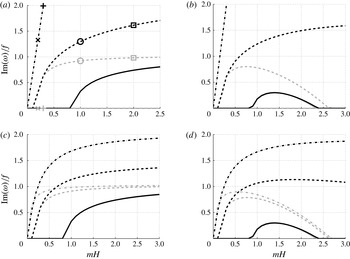
. Eigenproblems (3.25) and (3.27) are numerically solved using the pseudo-spectral method described at the end of § 2.2. We investigated stratification, NH and dissipation effects by letting
 $N^{2}$
vary,
 ${\it\delta}_{NH}$
be equal either to zero or unity, and
 ${\it\nu}={\it\kappa}$
be either 0 or
 $10^{4}$
m
 $^{2}$
s
 $^{-1}$
. In the latter case, when
 ${\it\nu}\neq 0$
,
 ${\it\nu}^{2}$
should be large enough to counterbalance the term
 $k\overline{u}$
and to stabilize the flow at large vertical wavenumbers, i.e.
 ${\it\nu}\approx fH^{2}\approx 10^{4}$
m
 $^{2}$
s
 $^{-1}$
around the reference configuration.
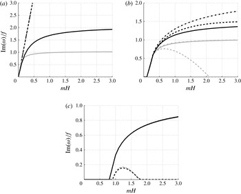
Dimensionless growth rate
 $\text{Im}({\it\omega})/f$
as a function of dimensionless vertical wavenumber
 $mH$
of the symmetric inertial instability at
 $N=0$
(dashed-dotted),
 $N=2f$
(dashed) and
 $N=10f$
(solid): (a)
 ${\it\delta}_{NH}=0$
,
 ${\it\nu}={\it\kappa}=0$
; (b)
 ${\it\delta}_{NH}=0$
,
 ${\it\nu}={\it\kappa}=10^{4}$
m
 $^{2}$
s
 $^{-1}$
; (c)
 ${\it\delta}_{NH}=1$
,
 ${\it\nu}={\it\kappa}=0$
; (d)
 ${\it\delta}_{NH}=1$
,
 ${\it\nu}={\it\kappa}=10^{4}$
m
 $^{2}$
s
 $^{-1}$
. The background jet corresponds to the reference configuration of table 1. Grey, TA (
 ${\it\delta}_{NT}=0$
); black, NT (
 ${\it\delta}_{NT}=0$
). Modes corresponding to
 $\times$
(
 $N=0,~mH=0.2$
),
 $+$
(
 $N=0,mH=0.3$
), ○ (
 $N=2f,mH=1$
) and ▫ (
 $N=2f,mH=1$
) are plotted in figure 11.

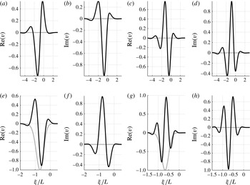
Eigenmodes
 $v$
of the symmetric inertial stability problem in the hydrostatic non-dissipative case as functions of
 ${\it\xi}/L$
. (a,b) Eigenmodes at neutral stratification
 $N=0$
with
 $mH=0.2$
, corresponding to
 $\times$
in figure 10(a). (c,d) Eigenmodes at neutral stratification
 $N=0$
with
 $mH=0.3$
, corresponding to
 $+$
in figure 10(a). (e,f) Eigenmodes at weak stratification
 $N=2f$
with
 $mH=1$
, corresponding to ○ in figure 10(a). (g,h) Eigenmodes at weak stratification
 $N=2f$
with
 $mH=2$
, corresponding to ▫ in figure 10(a). Grey, TA (
 ${\it\delta}_{NT}=0$
); black, NT (
 ${\it\delta}_{NT}=0$
).

The growth rates of the instability in the reference configuration as a function of vertical wavenumber
 $m$
are plotted in figure 10 for three different values of the Brunt–Väisälä frequency, corresponding to neutral
 $N=0$
, weak
 $N=2f$
and strong
 $N=10f$
stratifications. The results are presented in four different cases: (a) hydrostatic non-dissipative,
 ${\it\delta}_{NH}=0$
and
 ${\it\nu}={\it\kappa}=0$
; (b) hydrostatic dissipative,
 ${\it\delta}_{NH}=0$
and
 ${\it\nu}={\it\kappa}=10^{4}$
m
 $^{2}$
s
 $^{-1}$
; (c) NH non-dissipative,
 ${\it\delta}_{NH}=1$
and
 ${\it\nu}={\it\kappa}=0$
; and (d) NH dissipative,
 ${\it\delta}_{NH}=1$
and
 ${\it\nu}={\it\kappa}=10^{4}$
m
 $^{2}$
s
 $^{-1}$
. As a consistency check, we benchmarked our numerical results with analytic estimates of § 3.3.1. We obtained very good matches with calculated eigenfrequencies in all cases. The results are as follows:
-
(a) Hydrostatic non-dissipative case
 ${\it\delta}_{NH}=0$
,
${\it\nu}={\it\kappa}=0$
. For neutral stratification, as expected from the analytical results, the jet under the TA is inertially stable, while it is unstable relaxing the TA. In the latter case, the growth rate is proportional to the vertical wavenumber
$m$
. For a weak stratification (
$N=2f$
), the jet is inertially unstable in both approximations, but the NT growth rate is significantly larger than its traditional counterpart for all values of vertical wavenumber. For low enough vertical wavenumbers, the jet is stable with and without the TA, as expected from integral estimates. For larger
$m$
, the relative difference between traditional and NT growth rates can become almost 100 %, depending on stratification. However, at sufficiently large
$N$
, the difference between traditional and NT instabilities becomes indiscernible.
-
(b) Hydrostatic dissipative case
${\it\delta}_{NH}=0$
,
${\it\nu}={\it\kappa}=10^{4}$
m
$^{2}$
s
$^{-1}$
. For long waves and for the neutral stratification, dissipation has no effects on the growth rate when relaxing the TA. For weak but non-zero stratification, as within the TA, there is a threshold in vertical wavenumber for the instability. Dissipation allows for selection of the most unstable mode. Otherwise as
$m\rightarrow \infty$
, the growth rate becomes independent of
$m$
. When the TA is relaxed, the interval of vertical wavenumbers of unstable modes becomes larger. -
(c) Non-hydrostatic non-dissipative case
${\it\delta}_{NH}=1$
,
${\it\nu}={\it\kappa}=0$
. The jet is unstable with and without the TA, but the growth rates are larger when relaxing the TA. The relative difference between the growth rates increases with decreasing stratification. The behaviour of the growth rates is therefore similar to what was observed for
${\it\delta}_{NH}=0$
and
${\it\nu}={\it\kappa}=0$
, and is consistent with corresponding integral estimates. -
(d) Non-hydrostatic dissipative case
${\it\delta}_{NH}=1$
,
${\it\nu}={\it\kappa}=10^{4}$
m
$^{2}$
s
$^{-1}$
. For neutral (
$N=0$
) and weak (
$N=2f$
) stratifications, the stabilizing role of dissipation is much less pronounced without the TA. For strong stratifications (
$N=10f$
), NT and traditional growth rates practically coincide, and the jet is stable for
$mH\geqslant 2.4$
.


Dimensionless growth rate
 $\text{Im}({\it\omega})/f$
of the symmetric inertial instability as a function of dimensionless vertical wavenumber
 $mH$
for
 ${\it\delta}_{NH}=0,{\it\nu}=0$
(dashed-dotted),
 ${\it\delta}_{NH}=0,{\it\nu}=10^{4}$
m
 $^{2}$
s
 $^{-1}$
(dashed),
 ${\it\delta}_{NH}=1,{\it\nu}=0$
(solid): (a)
 $N=0$
, (b)
 $N=2f$
, (c)
 $N=10f$
. Grey, TA (
 ${\it\delta}_{NT}=0$
); black, NT (
 ${\it\delta}_{NT}=0$
). Background flow in the reference configuration of table 1.

We investigated how the NT terms affect the structure of the unstable modes in the hydrostatic non-dissipative case (
 ${\it\delta}_{NH}=0,~{\it\nu}={\it\kappa}=0$
), when the stability problem is formulated in terms of (3.31). The real and imaginary parts of the meridional velocity
 $v$
of unstable modes are plotted in figure 11 as functions of
 ${\it\xi}$
, at neutral (
 $N=0$
) and weak (
 $N=2f$
) stratifications. The modes, respectively, correspond to the cross (
 $mH=0.2$
), plus (
 $mH=0.3$
), circle (
 $mH=1$
) and square (
 $mH=2$
) in figure 10. At neutral stratification, the NT unstable mode is trapped in the region of negative PV, while the eigenmode under the TA is identically zero and the jet is stable, as already discussed above in § 3.3.1. Figure 11(e–h) show
 $\text{Re}(v)$
and
 $\text{Im}(v)$
at
 $N=2f$
for two different values of vertical wavenumber:
 $mH=1$
and
 $mH=2$
. The traditional unstable modes have zero imaginary part, while the imaginary part of the NT modes is non-zero due to the complex character of the modified Sturm–Liouvile problem (3.31). Another surprising result in the modified Sturm–Liouville problem is that, following the curve of the growth rate
 $\text{Im}({\it\omega})$
as a function of
 $m$
, the number of nodes of the corresponding NT mode increases, while it remains the same with the TA. As seen in the bottom panels of the figure, for example, NT
 $\text{Re}(v)$
has three, then five nodes, while it has no nodes under the TA.
We now compare the behaviour of the growth rates at a given value of
 $N$
in three cases: (a)
 ${\it\delta}_{NH}=0$
and
 ${\it\nu}={\it\kappa}=0$
; (b)
 ${\it\delta}_{NH}=0$
and
 ${\it\nu}={\it\kappa}=10^{4}$
m
 $^{2}$
s
 $^{-1}$
; (c)
 ${\it\delta}_{NH}=1$
and
 ${\it\nu}={\it\kappa}=0$
. The growth rates of the symmetric inertial instability are plotted in figure 12 as functions of vertical wavenumber
 $m$
. The results are as follows:
-
(a) Neutral stratification
$N=0$
. As noted earlier, dissipation does not have significant influence upon the vertical scale selection when relaxing the TA in the hydrostatic limit. By relaxing the hydrostatic approximation, the NT growth rate saturates at large
$m$
, while it is going to infinity when
$m\rightarrow \infty$
for
${\it\delta}_{NH}=0$
, as follows from (3.47). -
(b) Weak stratification
$N=2f$
. Unlike the TA, NH and hydrostatic instabilities do not have close growth rates. Without the TA, the NH effects counterbalance the NT effects and tend to saturate the growth rate even more efficiently than dissipation. -
(c) Strong stratification
$N=10f$
. No significant differences are observed between the growth rates with and without the TA.


As a preliminary conclusion we can state that the numerical results are fully consistent with available analytical estimates and that we observe substantial differences in values of the growth rates and their dependence on parameters, with and without the TA. In particular, the dissipation, for weak stratifications (
 $N\lesssim f$
), has only a limited impact on the NT growth rate, in contrast to the TA. Nevertheless, these differences diminish and then disappear with increasing stratification. An important result is that the across-jet structure of the unstable modes is substantially different without the TA with more nodes, and hence stronger meridional gradients, which is important in the saturation process. It should be emphasized that such a difference between traditional and NT unstable modes was not observed in the two-layer model.
3.4. Results of the linear stability analysis of the asymmetric problem
We now present numerical results for the asymmetric problem with
 $k\neq 0$
. As in the previous section, we consider the general eigenproblem (3.27) at neutral, weak and strong stratifications. We give results in each case for a given value of the vertical wavenumber, as the dependence on this latter was already investigated in the previous section. Thus, we will take (
 $N=0,mH=0.2$
) for neutral stratification, (
 $N=2f$
,
 $mH=1$
) for weak stratification and (
 $N=10f$
,
 $mH=1$
) for strong stratification. We investigate the role of NH effects.
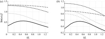
Growth rates corresponding to the chosen stratifications and vertical wavenumbers are plotted in figure 13 as functions of the dimensionless zonal wavenumber
 $kL$
. For neutral or weak stratification, the NT growth rate remains substantially higher than under the TA. In both approximations (modulo the fact that under the TA the flow is stable at
 $N=0$
), the growth rate has a maximum at
 $k=0$
, i.e. for the symmetric instability. While the differences between the traditional and NT growth rates are quite significant for weak stratifications, they become indiscernible for large enough
 $N$
. This is consistent with the results presented in § 3.3. NH effects tend to stabilize the flow for any zonal wavenumber. At high
 $k$
, the stabilization is more efficient with that without the TA concerning the neutral stratification case.
Dimensionless growth rate
 $\text{Im}({\it\omega})/f$
as a function of dimensionless zonal wavenumber
 $k$
for
 $N=0$
,
 $mH=0.2$
(dashed-dotted),
 $N=2f$
,
 $mH=1$
(dashed) and
 $N=10f$
,
 $mH=1$
(solid): (a)
 ${\it\delta}_{NH}=0$
,
 ${\it\nu}={\it\kappa}=0$
; (b)
 ${\it\delta}_{NH}=1$
,
 ${\it\nu}={\it\kappa}=0$
. Grey, TA (
 ${\it\delta}_{NT}=0$
); black, NT (
 ${\it\delta}_{NT}=0$
).

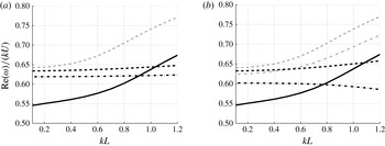
The phase velocities of the unstable modes are plotted in figure 14 as functions of
 $kL$
. Under the TA, no significant difference between hydrostatic and NH regimes is noted (modulo the fact that under the TA the flow is stable at
 $N=0$
). The phase velocity increases as zonal wavenumber increases and the phase velocity with the TA is uniform in the limit
 $k\rightarrow 0$
(Griffiths Reference Griffiths2008; Ribstein et al.
Reference Ribstein, Plougonven and Zeitlin2014a
). While relaxing the TA, except for neutral stratification,
 $\text{Re}({\it\omega})/k$
increases as
 $k$
increases, at a much slower rate than with the TA concerning weak stratifications. The NT phase velocity is always weaker than its traditional counterpart. Concerning the neutral case, when
 ${\it\delta}_{NH}=0$
, the NT phase velocity remains quasi-constant for all
 $k$
. While relaxing the hydrostatic approximation, the NT phase velocity surprisingly decreases as
 $k$
increases.
Dimensionless phase speed of the asymmetric modes of inertial instability
 $\text{Re}({\it\omega})/(kU)$
as a function of dimensionless zonal wavenumber
 $kL$
for
 $N=0$
,
 $mH=0.2$
(dashed-dotted),
 $N=2f$
,
 $mH=1$
(dashed) and
 $N=10f$
,
 $mH=1$
(solid): (a)
 ${\it\delta}_{NH}=0$
,
 ${\it\nu}={\it\kappa}=0$
; (b)
 ${\it\delta}_{NH}=1$
,
 ${\it\nu}={\it\kappa}=0$
. Grey, TA (
 ${\it\delta}_{NT}=0$
); black, NT (
 ${\it\delta}_{NT}=0$
).

The influence of dissipation and vertical wavenumber on the asymmetric instability was also investigated. As expected, dissipation stabilizes the flow for any zonal wavenumbers
 $k$
, starting from some cut-off vertical wavenumber
 $m_{c}$
, both with and without the TA. In the case of neutral stratification, dissipation has almost no effect on the behavior of the growth rate as a function of
 $k$
for the chosen vertical wavenumber (
 $mH=0.2$
, see also figure 10
a). Under hydrostatic and traditional approximations, the dissipation terms
 $\text{i}{\it\nu}m^{2}$
are not coupled to the zonal wavenumber
 $k$
in the eigenproblem, and stabilization is monotonic in
 ${\it\nu}$
. When relaxing the hydrostatic or traditional approximations, the dissipation terms break the symmetry of the eigenproblem and are coupled with
 $k$
. Then adding dissipation produces a surprising effect of increasing the difference between the traditional and NT growth rates (the highest one being NT) at strong stratifications (
 $N=10f$
), which becomes non-negligible (around 15 % of the relative difference).
Growth rate
 $\text{Im}({\it\omega})$
increases as
 $m$
increases for any
 $k$
both with and without the TA. For strong stratifications (
 $N=10f$
) and
 $mH=1$
, the highest growth rate is reached at non-zero
 $k$
. With increasing
 $m$
, the symmetric growth rate becomes the most unstable one. Except for the neutral case, phase velocity
 $\text{Re}({\it\omega})/k$
increases as
 $m$
increases for any
 $k$
in both hydrostatic and NH regimes. When
 $N=0$
and
 ${\it\delta}_{NH}=0$
,
 $\text{Re}({\it\omega})/k$
decreases as
 $m$
increases for any
 $k$
. While relaxing the hydrostatic approximation, phase velocity increases as
 $m$
increases for any
 $k$
. For sufficiently large
 $m$
(from
 $mH\approx 0.5$
), it increases as
 $k$
increases.
3.5. Preliminary conclusions in the continuously stratified case
For neutral and weak stratifications, the NT growth rates are much larger than under the TA through the whole range of zonal wavenumbers
 $k$
we have studied, while at strong stratifications they tend to coincide for all
 $k$
. Both dissipation and NH effects tend to diminish the growth rate at larger
 $k$
, their influence being stronger with than without the TA. The phase speed of the unstable mode increases with decreasing stratification and tends to increase with the zonal wavenumber for non-neutral stratifications. The across-jet structure of unstable modes is different without the TA.
4. Summary and discussion
We performed a detailed linear stability analysis of a mid-latitude barotropic Bickley jet for long-wave perturbations, both in two-layer rotating shallow-water and continuously stratified models on the NT
 $f$
-plane. As the NT effects are expected to manifest themselves at weak stratifications, we investigated the influence of stratification on the instabilities, the stratification being controlled by the density ratio
 $r$
or the baroclinic Burger number
 $\mathit{Bu}^{\ast }=(\sqrt{g(1-r)H}/(\,fL))^{2}$
in the two-layer model and by the Brunt–Väisälä frequency
 $N$
or the baroclinic Burger number
 $\mathit{Bu}^{\ast }=(NH/(\,fL))^{2}$
in the continuously stratified model. In the latter, we have also considered the influence of NH effects, while layered models are hydrostatic by construction. Our principal results are as follows.
Two-layer shallow-water model. As under the TA, the NT growth rate increases with
 $\mathit{Ro},r,d$
, and decreases with
 $\mathit{Bu}$
. The NT symmetric instability has a higher growth rate than under the TA for all values of parameters
 $\mathit{Bu},\mathit{Ro},d$
and
 $r$
(with relative difference of 10–20 %). There exists a range of parameters where the jet is inertially unstable without the TA, while it is stable with the TA. The asymmetric inertial instability has also a higher NT growth rate. The maximum of the growth rate of inertial instability is at small but non-zero zonal wavenumber, like under the TA, but with a smaller zonal wavenumber. The NT unstable modes have higher phase velocities for long-wave perturbations, as compared to the TA. The across-jet structure of the unstable modes is the same with and without the TA.
Continuously stratified Boussinesq model. Relaxing the TA in this model changes profoundly the structure of the stability problem. Because of the misalignment between the gravity acceleration and the rotation vector on the NT
 $f$
-plane, the stability problem becomes non-separable, which substantially increases the technical difficulties. However, we found a change of variables that renders the problem separable. In this way, as under the TA, it can be treated by a Fourier transform in time, zonal and vertical coordinates, which reduces the problem to a system of ODEs, which, in turn, may be discretized and analysed numerically for any jet profile. Yet, the change of meridional variable leads to unusual structure of dissipative terms, which become non-diagonal after discretization and need special care, if the role of dissipation is to be studied. Our analysis included both hydrostatic and NH versions of the model with and without dissipation.
As in the two-layer model, the NT growth rate of the symmetric instability is higher than under the TA, with a relative difference that can reach more than 100 % at weak stratifications. The neutral stratification is a particular case as in the hydrostatic limit the jet is inertially stable under the TA, while the instability is present relaxing the TA. The growth rate of the instability increases linearly with the vertical wavenumber. Relaxing the hydrostatic approximation at non-neutral stratification has no significant effect upon the traditional growth rate, while it leads to the saturation of the NT growth rate at large enough vertical wavenumbers. Then NH effects are shown to have a considerable effect upon the instability while relaxing the TA. The dissipation has a well-known scale selection effect under the TA. The same effect is observed when relaxing the TA. However, at a given dissipation the NT effects enlarge the vertical scale range in which the flow is inertially unstable.
In both models, the results are qualitatively similar: the NT growth rate of symmetric and/or asymmetric instabilities is higher than under the TA, with a larger relative difference in the continuously stratified model. The phase velocity of the unstable modes increases with the zonal wavenumber. In similar parameter ranges, which corresponds to small vertical wavenumbers and hydrostatic limit in the continuously stratified case, the asymmetric instability always has the highest growth rate. An essential difference between the two-layer and continuously stratified models however is that symmetric instability becomes dominant at high enough vertical wavenumbers in the latter. Another difference is due to non-hydrostatic effects, which are absent by definition in the two-layer model and tend to diminish the growth rate of the instability in the continuously stratified model.
The linear stability analysis of this paper was performed on the
 $f$
-plane. Yet, as discussed in the introduction, the equatorial region is a privileged place for NT effects to show up, and the question of extension to the equatorial
 ${\it\beta}$
-plane arises. Concerning the continuously stratified model, the change of variable used in § 3 will become
 ${\it\xi}={\it\beta}y^{2}/2-Fz$
on the equatorial
 ${\it\beta}$
-plane. Owing to the horizontal dependence of the traditional Coriolis parameter
 $f={\it\beta}y=\sqrt{2{\it\beta}({\it\xi}+Fz)}$
, the problem thus remains non-separable even for barotropic jets, and a discretization in the two directions
 $y$
and
 $z$
seems to be inevitable, with subsequent technical complications.
Our linear results allow us to make some predictions on the saturation of the instability. The different structure of unstable modes with and without the TA implies that saturation rates and patterns are different. For example, the fact that the NT mode is more sheared horizontally allows us to suppose that this could lead to the increase of horizontal mixing. In general the very fact that the growth rates of inertial instability are higher without the TA means that mixing, which is typically produced at its nonlinear stage, becomes faster and stronger. In order to quantify such effects, reliable high-resolution numerical codes are necessary. Building a consistent numerical scheme in NT approximation is a non-trivial task. For example, in the NT rotating shallow-water models the non-conservative NT terms, even in the one-layer configuration, are problematic in the finite-volume numerical methods, which were successfully used with the TA. The work on numerical simulations of developing NT instabilities is in progress and will be presented elsewhere.
In recent years, sensitivity to NT effects was revealed in various dynamical phenomena. Perhaps the most important message we want to deliver is that NT effects can change the instability patterns both quantitatively and qualitatively and thus must be taken into account.
Acknowledgements
This work was partially supported by the Institut Universitaire de France. B.R. thanks the German Federal Ministry of Education and Research (BMBF) for support through the program Role of the Middle Atmosphere in Climate (ROMIC) and through grant 01LG1220A. The authors are grateful to four anonymous referees for their remarks, which helped to improve the presentation.