



1 Introduction
There is no doubt that the first two similarity hypotheses of Kolmogorov (Reference Kolmogorov1941a
,Reference Kolmogorov
b
), widely known as K41, and Kolmogorov’s (Reference Kolmogorov1962) refined similarity hypothesis, known as K62, which was introduced to account for the so-called ‘internal intermittency’, have had a huge impact on turbulence research. According to K41, small-scale statistics should adopt particular universal forms when the focus is on small scales or scales lying within the dissipative and inertial ranges. For example, the Kolmogorov-normalized one-dimensional velocity spectra
 $\unicode[STIX]{x1D719}_{u}^{\ast }(k_{1}^{\ast })$
(the asterisk denotes normalization by the Kolmogorov length scale,
 $\unicode[STIX]{x1D702}=(\unicode[STIX]{x1D708}^{3}/\overline{\unicode[STIX]{x1D716}})^{1/4}$
, where
 $\unicode[STIX]{x1D708}$
is the kinematic viscosity of the fluid,
 $\overline{\unicode[STIX]{x1D716}}$
is the mean turbulent energy dissipation rate, and the overbar denotes time averaging, and/or Kolmogorov velocity scale,
 $u_{K}=(\unicode[STIX]{x1D708}\overline{\unicode[STIX]{x1D716}})^{1/4}$
) collapse in the high-wavenumber region (Saddoughi & Veeravalli Reference Saddoughi and Veeravalli1994). Antonia, Djenidi & Danaila (Reference Antonia, Djenidi and Danaila2014) showed that this collapse is consistent with the Navier–Stokes (NS) equations and does not require the Reynolds number to be large, nor does it require local isotropy to be rigorously satisfied, i.e. the constraints imposed by K41 can be relaxed significantly.
For the velocity structure functions, the first similarity hypothesis of K41 predicts
 $$\begin{eqnarray}\overline{(\unicode[STIX]{x1D6FF}u^{\ast })^{n}}=f_{un}(r^{\ast }),\end{eqnarray}$$
with the velocity increment
 $\unicode[STIX]{x1D6FF}u=u(x+r)-u(x)$
between two points separated by a distance
 $r$
along
 $x$
, the flow direction;
 $f_{un}$
is a universal function when normalized by
 $\unicode[STIX]{x1D702}$
and/or
 $u_{K}$
for each value of
 $n$
. When
 $r\rightarrow 0$
, (1.1) leads to
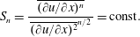 $$\begin{eqnarray}S_{n}=\frac{\overline{(\unicode[STIX]{x2202}u/\unicode[STIX]{x2202}x)^{n}}}{\,\overline{(\unicode[STIX]{x2202}u/\unicode[STIX]{x2202}x)^{2}}^{n/2}\,}=\text{const}.\end{eqnarray}$$
for each value of
 $n$
at large
 $Re_{\unicode[STIX]{x1D706}}$
(
 $=u^{\prime }\unicode[STIX]{x1D706}/\unicode[STIX]{x1D708}$
, where
 $\unicode[STIX]{x1D706}$
is the longitudinal Taylor microscale
 $u^{\prime }/(\unicode[STIX]{x2202}u/\unicode[STIX]{x2202}x)^{\prime }$
and a prime denotes a root-mean-square value). According to K41, the constant associated with each
 $n$
should be universal.
Many studies have focused on the evolution of
 $S_{n}$
with
 $Re_{\unicode[STIX]{x1D706}}$
, with the view to test K41 and K62. With few exceptions (Tabeling et al.
Reference Tabeling, Zocchi, Belin, Maurer and Willaime1996; Belin et al.
Reference Belin, Maurer, Tabeling and Willaime1997), there has been strong support for the argument that
 $|S_{n}|$
(
 $n\geqslant 3$
) can increase continuously with
 $Re_{\unicode[STIX]{x1D706}}$
, viz.
 $$\begin{eqnarray}|S_{n}|\sim Re_{\unicode[STIX]{x1D706}}^{\unicode[STIX]{x1D6FC}_{n}}\quad (\unicode[STIX]{x1D6FC}>0)\end{eqnarray}$$
(see e.g. Gibson, Stegen & Williams Reference Gibson, Stegen and Williams1970; Wyngaard & Tennekes Reference Wyngaard and Tennekes1970; Van Atta & Antonia Reference Van Atta and Antonia1980; Antonia, Chambers & Satyaprakash Reference Antonia, Chambers and Satyaprakash1981; Antonia, Satyaprakash & Hussain Reference Antonia, Satyaprakash and Hussain1982; Sreenivasan & Antonia Reference Sreenivasan and Antonia1997; Davidson Reference Davidson2004; Ishihara et al.
Reference Ishihara, Kaneda, Yokokawa, Itakura and Uno2007; Ishihara, Gotoh & Kaneda Reference Ishihara, Gotoh and Kaneda2009; Wyngaard Reference Wyngaard2010). However, it appears now that not only are the small-scale statistics affected by
 $Re_{\unicode[STIX]{x1D706}}$
(this is the so-called finite-Reynolds-number (FRN) effect, which is inextricably linked with the large-scale forcing in a specific flow), but also the approach towards an asymptotic state as
 $Re_{\unicode[STIX]{x1D706}}$
increases differs from flow to flow (Thiesset, Antonia & Djenidi Reference Thiesset, Antonia and Djenidi2014; Antonia et al.
Reference Antonia, Tang, Djenidi and Danaila2015, Reference Antonia, Djenidi, Danaila and Tang2017). These results strongly indicate that the
 $Re_{\unicode[STIX]{x1D706}}$
dependence of
 $S_{n}$
should be revisited. In particular, this dependence should be assessed separately in each flow. Such attempts have already been initiated by Antonia et al. (Reference Antonia, Tang, Djenidi and Danaila2015) and Tang et al. (Reference Tang, Antonia, Djenidi, Abe, Zhou, Danaila and Zhou2015a
,Reference Tang, Antonia, Djenidi and Zhou
b
), who, starting from the NS equations, developed the locally isotropic form of the transport equation for
 $\overline{\unicode[STIX]{x1D716}}$
in the following flows: grid turbulence; along the axis in the self-preserving far field of a round jet; along the centrelines of a fully developed channel flow; and the far wake of a circular cylinder. They further showed that, in each flow they considered, the transport equation for
 $\overline{\unicode[STIX]{x1D716}}$
can be expressed in the generic form
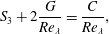 $$\begin{eqnarray}S_{3}+2\frac{G}{Re_{\unicode[STIX]{x1D706}}}=\frac{C}{Re_{\unicode[STIX]{x1D706}}},\end{eqnarray}$$
where
 $G$
is the non-dimensional enstrophy destruction coefficient of
 $\overline{\unicode[STIX]{x1D716}}$
defined as
 $$\begin{eqnarray}G=\overline{u^{2}}\,\frac{\,\overline{(\unicode[STIX]{x2202}^{2}u/\unicode[STIX]{x2202}x^{2})^{2}}\,}{\overline{(\unicode[STIX]{x2202}u/\unicode[STIX]{x2202}x)^{2}}^{2}}.\end{eqnarray}$$
(Note that Batchelor & Townsend (Reference Batchelor and Townsend1947) first derived (1.4) for grid turbulence.) It was also shown that the analytical expressions for
 $C$
differ from flow to flow. Further, since
 $2G/Re_{\unicode[STIX]{x1D706}}$
was found to be very nearly constant for
 $Re_{\unicode[STIX]{x1D706}}\geqslant 70{-}100$
,
 $S_{3}$
approaches what appears to be a universal constant (
 ${\approx}0.53$
) when
 $Re_{\unicode[STIX]{x1D706}}$
is sufficiently large, but the way this constant is approached is flow-dependent. In fact,
 $Re_{\unicode[STIX]{x1D706}}$
only needs to exceed approximately 300 for
 $S_{3}$
to be considered constant for all the experimental data in flows considered in the above studies and direct numerical simulations (DNS) of turbulence in a periodic box (Kerr Reference Kerr1985; Jimenez et al.
Reference Jimenez, Wray, Saffman and Rogallo1993; Yeung & Zhou Reference Yeung and Zhou1997; Gotoh, Fukayama & Nakano Reference Gotoh, Fukayama and Nakano2002; Yeung, Donzis & Sreenivasan Reference Yeung, Donzis and Sreenivasan2005). A notable exception to this behaviour comes from the data by Ishihara et al. (Reference Ishihara, Kaneda, Yokokawa, Itakura and Uno2007) and Gauding (Reference Gauding2014) for DNS of turbulence in a periodic box up to
 $Re_{\unicode[STIX]{x1D706}}=1131$
. This inconsistency has been discussed in detail by Antonia et al. (Reference Antonia, Tang, Djenidi and Danaila2015); we will revisit this issue later (§ 3) when discussing results for
 $S_{4}$
. For (1.1), Pearson & Antonia (Reference Pearson and Antonia2001) showed that
 $\overline{(\unicode[STIX]{x1D6FF}u^{\ast })^{2}}$
collapses in the dissipative range over a large range of
 $Re_{\unicode[STIX]{x1D706}}$
(
 $40<Re_{\unicode[STIX]{x1D706}}<4250$
) while Antonia et al. (Reference Antonia, Tang, Djenidi and Danaila2015) showed that
 $S_{\unicode[STIX]{x1D6FF}u}$
, the skewness of
 $\unicode[STIX]{x1D6FF}u$
, viz.
 $S_{\unicode[STIX]{x1D6FF}u}=\overline{(\unicode[STIX]{x1D6FF}u)^{3}}/\,\overline{(\unicode[STIX]{x1D6FF}u)^{2}}^{3/2}$
, becomes independent of
 $Re_{\unicode[STIX]{x1D706}}$
in the dissipative range when
 $Re_{\unicode[STIX]{x1D706}}$
is sufficiently large.
The existing evidence only verified the constancy of (1.2) (K41) for
 $n=3$
and the
 $Re_{\unicode[STIX]{x1D706}}$
independence of (1.1) (K41) in the dissipative range for
 $n=2,3$
. It now seems implausible that (1.1) and (1.2) will behave differently for
 $n>3$
at least in the dissipative range. In a recent paper, Antonia et al. (Reference Antonia, Djenidi, Danaila and Tang2017) examined the variation of
 $S_{n}$
with
 $Re_{\unicode[STIX]{x1D706}}$
, equation (1.2), up to
 $n=6$
, on the axis of a plane jet, and found that
 $S_{n}$
for
 $n=3$
to 6 is constant (by definition,
 $S_{2}=1$
) over a range
 $500<Re_{\unicode[STIX]{x1D706}}<1100$
, implying that the FRN effect is no longer present beyond
 $Re_{\unicode[STIX]{x1D706}}\approx 500$
. The authors further examined
 $\overline{(\unicode[STIX]{x1D6FF}u^{\ast })^{n}}$
(
 $n=2{-}6$
) for the plane jet data at
 $Re_{\unicode[STIX]{x1D706}}=550$
, 696, 826, 914 and 1067, respectively, and found that there is relatively good collapse for all the structure functions at small
 $r^{\ast }$
(dissipative range). They also pointed out that all these results associated with the dissipative range favour K41 over K62 and hence imply that intermittency-related corrections are not needed at large
 $Re_{\unicode[STIX]{x1D706}}$
.
The work reported above focused only on assessing the FRN effect on the behaviour of
 $S_{3}$
in several turbulent flows. To our knowledge, however, there has been no attempt to examine the FRN effect on
 $S_{4}$
separately in each flow. Accordingly, the present paper, which complements and extends our earlier examination of
 $S_{3}$
(Antonia et al.
Reference Antonia, Tang, Djenidi and Danaila2015) aims at filling this gap. It has two major objectives:
(i) In § 2, starting from the NS equations, we derive an expression for the derivative flatness factor
 $S_{4}$
and argue that
 $S_{4}$
should, like
 $S_{3}$
, be bounded when
 $Re_{\unicode[STIX]{x1D706}}$
is sufficiently large.
(ii) In § 3, we examine critically the data for
 $S_{4}$
, as reported in the literature and new experimental data, in the light of the FRN effect. It is plausible that, at low to moderate
 $Re_{\unicode[STIX]{x1D706}}$
,
 $S_{4}$
, like
 $S_{3}$
, differs from flow to flow and exhibits a
 $Re_{\unicode[STIX]{x1D706}}$
dependence until it approaches a constant when
 $Re_{\unicode[STIX]{x1D706}}$
is sufficiently large. This trend appears to be adequately corroborated by the laboratory data considered in this paper. Further, the reasons why the atmospheric surface layer (ASL) data should be discarded when testing K41 and K62 are discussed briefly at the end of § 3.
2 Theoretical considerations
Since the main interest of this paper is the behaviour of the flatness factor of the velocity derivative, an appropriate starting point is the transport equation for the third-order structure function (Hill Reference Hill2001), tenable under the assumptions of local homogeneity and isotropy:
 $$\begin{eqnarray}\underbrace{\unicode[STIX]{x2202}_{t}D_{111}}_{\text{term}\,1}+\underbrace{\left(\unicode[STIX]{x2202}_{r}+\frac{2}{r}\right)D_{1111}}_{\text{term}\,2}-\underbrace{\frac{6}{r}D_{1122}}_{\text{term}\,2^{\prime }}=\underbrace{-T_{111}}_{\text{term}\,3}+\underbrace{2\unicode[STIX]{x1D708}C}_{\text{term}\,4}-\underbrace{2\unicode[STIX]{x1D708}Z_{111}}_{\text{term}\,5},\end{eqnarray}$$
with
 $\unicode[STIX]{x2202}_{r}\equiv \unicode[STIX]{x2202}/\unicode[STIX]{x2202}r$
,
 $$\begin{eqnarray}\displaystyle \left.\begin{array}{@{}c@{}}\displaystyle D_{111}=\overline{(\unicode[STIX]{x1D6FF}u)^{3}},\\ \displaystyle D_{1111}=\overline{(\unicode[STIX]{x1D6FF}u)^{4}},\\ \displaystyle D_{1122}=\overline{(\unicode[STIX]{x1D6FF}u)^{2}(\unicode[STIX]{x1D6FF}v)^{2}},\\ \displaystyle C(r,t)=-\frac{4}{r^{2}}D_{111}(r,t)+\frac{4}{r}\unicode[STIX]{x2202}_{r}D_{111}+\unicode[STIX]{x2202}_{r}\unicode[STIX]{x2202}_{r}D_{111},\\ \displaystyle Z_{111}=3\,\overline{\unicode[STIX]{x1D6FF}u\left[\left(\frac{\unicode[STIX]{x2202}u}{\unicode[STIX]{x2202}x_{l}}\right)^{2}+\left(\frac{\unicode[STIX]{x2202}u^{\prime }}{\unicode[STIX]{x2202}x_{l}^{\prime }}\right)^{2}\right]},\end{array}\right\} & & \displaystyle\end{eqnarray}$$
where double indices indicate summation and a prime denotes variables at point
 $x+r$
. Finally,
 $$\begin{eqnarray}T_{111}=3\,\overline{(\unicode[STIX]{x1D6FF}u)^{2}\unicode[STIX]{x1D6FF}\!\left(\frac{\unicode[STIX]{x2202}p}{\unicode[STIX]{x2202}x}\right)}.\end{eqnarray}$$
Terms 1 to 5 denote terms in (2.1). The next step is to consider the limiting form of these terms, for
 $r\rightarrow 0$
, by applying a Taylor series expansion up to the fifth order in
 $r$
. Because of homogeneity,
 $$\begin{eqnarray}\frac{\unicode[STIX]{x2202}}{\unicode[STIX]{x2202}x}\overline{\left(\frac{\unicode[STIX]{x2202}u}{\unicode[STIX]{x2202}x}\right)^{2}\left(\frac{\unicode[STIX]{x2202}^{2}u}{\unicode[STIX]{x2202}x^{2}}\right)}\equiv 0\quad \Rightarrow \quad 2\,\overline{\frac{\unicode[STIX]{x2202}u}{\unicode[STIX]{x2202}x}\left(\frac{\unicode[STIX]{x2202}^{2}u}{\unicode[STIX]{x2202}x^{2}}\right)^{2}}=-\overline{\left(\frac{\unicode[STIX]{x2202}u}{\unicode[STIX]{x2202}x}\right)^{2}\left(\frac{\unicode[STIX]{x2202}^{3}u}{\unicode[STIX]{x2202}x^{3}}\right)},\end{eqnarray}$$
and hence
 $$\begin{eqnarray}\overline{(\unicode[STIX]{x1D6FF}u)^{3}}\simeq \overline{\left(\frac{\unicode[STIX]{x2202}u}{\unicode[STIX]{x2202}x}\right)^{3}}r^{3}-\frac{1}{4}\overline{\frac{\unicode[STIX]{x2202}u}{\unicode[STIX]{x2202}x}\left(\frac{\unicode[STIX]{x2202}^{2}u}{\unicode[STIX]{x2202}x^{2}}\right)^{2}}r^{5}+\cdots \,.\end{eqnarray}$$
The fourth-order structure function can be written as
 $$\begin{eqnarray}D_{1111}=\overline{(\unicode[STIX]{x1D6FF}u)^{4}}\simeq \overline{\left(\frac{\unicode[STIX]{x2202}u}{\unicode[STIX]{x2202}x}\right)^{4}}r^{4}+\cdots\end{eqnarray}$$
and similarly
 $$\begin{eqnarray}D_{1122}=\overline{(\unicode[STIX]{x1D6FF}u)^{2}(\unicode[STIX]{x1D6FF}v)^{2}}\simeq \overline{\left(\frac{\unicode[STIX]{x2202}u}{\unicode[STIX]{x2202}x}\right)^{2}\left(\frac{\unicode[STIX]{x2202}v}{\unicode[STIX]{x2202}x}\right)^{2}}r^{4}+\cdots \,.\end{eqnarray}$$
An equation for
 $S_{4}$
, the velocity derivative flatness factor, can be obtained by applying the following operator
 $O$
, defined as
 $$\begin{eqnarray}O\equiv \lim _{r\rightarrow 0}\frac{\,\displaystyle \frac{\text{terms in (2.1)}}{r^{3}}\,}{\displaystyle \frac{\,\overline{(\unicode[STIX]{x1D6FF}u)^{2}}^{2}\,}{r^{4}}}=\lim _{r\rightarrow 0}r\cdot \frac{\text{terms in (2.1)}}{\overline{(\unicode[STIX]{x1D6FF}u)^{2}}^{2}}.\end{eqnarray}$$
Term 1 in (2.1) represents a large-scale effect. It is written here as the temporal decay of
 $\overline{(\unicode[STIX]{x1D6FF}u)^{3}}$
, but more general forms may include a production of
 $\overline{(\unicode[STIX]{x1D6FF}u)^{3}}$
. For convenience, this term will be called
 $LS(r)$
(‘large scale’), which can be written as
 $$\begin{eqnarray}LS(r)=\frac{\unicode[STIX]{x2202}}{\unicode[STIX]{x2202}t}\overline{(\unicode[STIX]{x1D6FF}u)^{3}}=\left(\frac{\unicode[STIX]{x2202}}{\unicode[STIX]{x2202}t}u_{K}^{3}\right)\left(\frac{\,\overline{(\unicode[STIX]{x1D6FF}u)^{3}}\,}{u_{K}^{3}}\right)-u_{K}^{3}\frac{\unicode[STIX]{x2202}}{\unicode[STIX]{x2202}r^{\ast }}(\overline{(\unicode[STIX]{x1D6FF}u^{\ast })^{3}})r^{\ast }\frac{1}{\unicode[STIX]{x1D702}}\frac{\text{d}\unicode[STIX]{x1D702}}{\text{d}t}.\end{eqnarray}$$
We recall that, for decaying homogeneous and isotropic turbulence (HIT), the transport equation for the total kinetic energy
 $\overline{q^{2}}$
(
 $=\overline{u^{2}}+\overline{v^{2}}+\overline{w^{2}}$
) is given by
 $$\begin{eqnarray}\frac{1}{2}\frac{\unicode[STIX]{x2202}\overline{q^{2}}}{\unicode[STIX]{x2202}t}+\bar{\unicode[STIX]{x1D716}}=0,\end{eqnarray}$$
and
 $\overline{q^{2}}$
evolves in a power-law form during the decay, viz.
 $$\begin{eqnarray}\overline{q^{2}}\sim t^{n},\end{eqnarray}$$
where
 $n$
is the decaying exponent of the total kinetic energy. After substituting (2.11) in (2.10), we can obtain
 $\bar{\unicode[STIX]{x1D716}}\sim t^{n-1}$
. Further, using the definitions of
 $Re_{\unicode[STIX]{x1D706}}$
,
 $\unicode[STIX]{x1D702}$
and
 $u_{K}$
leads to
 $$\begin{eqnarray}\displaystyle \left.\begin{array}{@{}c@{}}Re_{\unicode[STIX]{x1D706}}\sim t^{n/2+1/2},\\ \unicode[STIX]{x1D702}\sim t^{(-n+1)/4},\\ u_{K}\sim t^{(n-1)/4}.\end{array}\right\} & & \displaystyle\end{eqnarray}$$
After substituting (2.12) in (2.9), the large-scale term can be written as
 $$\begin{eqnarray}\displaystyle O(LS) & = & \displaystyle \lim _{r\rightarrow 0}\left(r\frac{LS}{\,\overline{(\unicode[STIX]{x1D6FF}u)^{2}}^{2}\,}\right)=\lim _{r\rightarrow 0}\left(r\frac{(\unicode[STIX]{x2202}/\unicode[STIX]{x2202}t)\overline{(\unicode[STIX]{x1D6FF}u)^{3}}}{\,\overline{(\unicode[STIX]{x1D6FF}u)^{2}}^{3/2}\overline{(\unicode[STIX]{x1D6FF}u)^{2}}^{1/2}\,}\right)\nonumber\\ \displaystyle & = & \displaystyle \left(\frac{1-n}{2}\sqrt{\frac{15}{-n}}+10\frac{(1-n)}{-n}\right)\frac{S_{3}}{Re_{\unicode[STIX]{x1D706}}}.\end{eqnarray}$$
Because (i) the skewness of the velocity derivative,
 $S_{3}$
, is bounded (Antonia et al.
Reference Antonia, Tang, Djenidi and Danaila2015), and (ii)
 $n$
is finite with a value typically in the range
 $-$
1.5 to
 $-$
1.1 (e.g. Sinhuber, Bodenschatz & Bewley Reference Sinhuber, Bodenschatz and Bewley2015), the
 $O(LS)$
term will be increasingly less important as
 $Re_{\unicode[STIX]{x1D706}}$
increases.
It is straightforward to show that
 $O(\text{term 2})=S_{4}$
(because the operator
 $O$
was designed with this in mind). Similarly,
 $O(\text{term 2}^{\prime })=\overline{(\unicode[STIX]{x2202}u/\unicode[STIX]{x2202}x)^{2}(\unicode[STIX]{x2202}v/\unicode[STIX]{x2202}x)^{2}}/\,\overline{(\unicode[STIX]{x2202}u/\unicode[STIX]{x2202}x)^{2}}^{2}$
. For simplicity, we introduce
 $S_{uv,2}=\overline{(\unicode[STIX]{x2202}u/\unicode[STIX]{x2202}x)^{2}(\unicode[STIX]{x2202}v/\unicode[STIX]{x2202}x)^{2}}/\,\overline{(\unicode[STIX]{x2202}u/\unicode[STIX]{x2202}x)^{2}}^{2}$
.
The pressure term becomes, once
 $O$
is applied,
 $$\begin{eqnarray}O(\text{term 3})=-\frac{3\overline{\left(\displaystyle \frac{\unicode[STIX]{x2202}u}{\unicode[STIX]{x2202}x}\right)^{2}\displaystyle \frac{\unicode[STIX]{x2202}^{2}p}{\unicode[STIX]{x2202}x^{2}}}}{\overline{\displaystyle \left(\frac{\unicode[STIX]{x2202}u}{\unicode[STIX]{x2202}x}\right)^{2}}^{2}}=-3\times 15^{2}\,\overline{\left(\frac{\unicode[STIX]{x2202}u^{\ast }}{\unicode[STIX]{x2202}x^{\ast }}\right)^{2}\left(\frac{\unicode[STIX]{x2202}^{2}p^{\ast }}{\unicode[STIX]{x2202}x^{\ast 2}}\right)}.\end{eqnarray}$$
After applying the operator
 $O$
, term 4 leads to
 $-18\times 15^{2}\,\overline{(\unicode[STIX]{x2202}u^{\ast }/\unicode[STIX]{x2202}x^{\ast })(\unicode[STIX]{x2202}^{2}u^{\ast }/\unicode[STIX]{x2202}x^{\ast 2})^{2}}$
, or, equivalently,
 $9\times 15^{2}\,\overline{(\unicode[STIX]{x2202}u^{\ast }/\unicode[STIX]{x2202}x^{\ast })^{2}(\unicode[STIX]{x2202}^{3}u^{\ast }/\unicode[STIX]{x2202}x^{\ast 3})}$
. Term 5 leads to a linear combination of
 $15^{2}\,\overline{(\unicode[STIX]{x2202}^{3}u^{\ast }/\unicode[STIX]{x2202}x^{\ast 3})(\unicode[STIX]{x2202}u^{\ast }/\unicode[STIX]{x2202}x^{\ast })^{2}}$
and
 $2\times 15^{2}\,\overline{(\unicode[STIX]{x2202}^{3}u^{\ast }/\unicode[STIX]{x2202}x^{\ast 3})(\unicode[STIX]{x2202}u^{\ast }/\unicode[STIX]{x2202}y^{\ast })^{2}}$
. Since Djenidi et al. (Reference Djenidi, Antonia, Danaila and Tang2017b
) showed that
 $S_{uv,2}\approx 0.85S_{4}$
(using DNS data for HIT), the limiting form of (2.1) as
 $r\rightarrow 0$
can be finally expressed as
 $$\begin{eqnarray}S_{4}+\unicode[STIX]{x1D6FD}_{1}\overline{\left(\frac{\unicode[STIX]{x2202}u^{\ast }}{\unicode[STIX]{x2202}x^{\ast }}\right)^{2}\left(\frac{\unicode[STIX]{x2202}^{2}p^{\ast }}{\unicode[STIX]{x2202}x^{\ast 2}}\right)}+\unicode[STIX]{x1D6FD}_{2}\overline{\left(\frac{\unicode[STIX]{x2202}^{3}u^{\ast }}{\unicode[STIX]{x2202}x^{\ast 3}}\right)\left(\frac{\unicode[STIX]{x2202}u^{\ast }}{\unicode[STIX]{x2202}x^{\ast }}\right)^{2}}+\unicode[STIX]{x1D6FD}_{3}\overline{\left(\frac{\unicode[STIX]{x2202}^{3}u^{\ast }}{\unicode[STIX]{x2202}x^{\ast 3}}\right)\left(\frac{\unicode[STIX]{x2202}u^{\ast }}{\unicode[STIX]{x2202}y^{\ast }}\right)^{2}}=\unicode[STIX]{x1D6FD}_{4}\frac{S_{3}}{Re_{\unicode[STIX]{x1D706}}},\end{eqnarray}$$
where
 $\unicode[STIX]{x1D6FD}_{i}$
are dimensionless constants; the expressions and values for
 $\unicode[STIX]{x1D6FD}_{i}$
are shown in table 1. Equation (2.15) is the most general expression for the derivative flatness factor, as only local homogeneity and isotropy have been assumed. Note that Djenidi et al. (Reference Djenidi, Antonia, Danaila and Tang2017b
) have derived a similar equation for
 $S_{4}$
(see their equation (8)). However, the present (2.15) is more general and rigorous than their equation (8) for two reasons. First, they assume the flow is self-preserving; whilst it is relatively straightforward to show that the NS equations comply with this assumption (e.g. Antonia et al.
Reference Antonia, Djenidi and Danaila2014), it is best to avoid it altogether (note that this assumption was not used when testing the dependence of
 $S_{3}$
on
 $Re_{\unicode[STIX]{x1D706}}$
(see Antonia et al.
Reference Antonia, Tang, Djenidi and Danaila2015)). Second, for their equation (8), there is an inconsistency when using scaling variables since
 $S_{4}$
and
 $S_{uv,2}$
are normalized by Kolmogorov variables whereas the other quantities are normalized by
 $u^{\prime }$
and
 $\unicode[STIX]{x1D706}$
. Antonia et al. (Reference Antonia, Djenidi and Danaila2014) and Djenidi, Antonia & Danaila (Reference Djenidi, Antonia and Danaila2017a
) have already shown, by using the NS equations, that the Kolmogorov variables are the correct scaling parameters for the small-scale quantities, i.e. all terms in equation (8) of Djenidi et al. (Reference Djenidi, Antonia, Danaila and Tang2017b
) should have been normalized by Kolmogorov variables, as in (2.15).
Expressions and values for
 $\unicode[STIX]{x1D6FD}_{i}$
in (2.15).

We can rewrite (2.15) in a generic form as
 $$\begin{eqnarray}S_{4}+\unicode[STIX]{x1D6FE}=\unicode[STIX]{x1D6FD}\frac{S_{3}}{Re_{\unicode[STIX]{x1D706}}},\end{eqnarray}$$
where
 $$\begin{eqnarray}\unicode[STIX]{x1D6FE}\equiv \unicode[STIX]{x1D6FD}_{1}\overline{(\unicode[STIX]{x2202}u^{\ast }/\unicode[STIX]{x2202}x^{\ast })^{2}(\unicode[STIX]{x2202}^{2}p^{\ast }/\unicode[STIX]{x2202}x^{\ast 2})}+\unicode[STIX]{x1D6FD}_{2}\overline{(\unicode[STIX]{x2202}^{3}u^{\ast }/\unicode[STIX]{x2202}x^{\ast 3})(\unicode[STIX]{x2202}u^{\ast }/\unicode[STIX]{x2202}x^{\ast })^{2}}+\unicode[STIX]{x1D6FD}_{3}\overline{(\unicode[STIX]{x2202}^{3}u^{\ast }/\unicode[STIX]{x2202}x^{\ast 3})(\unicode[STIX]{x2202}u^{\ast }/\unicode[STIX]{x2202}y^{\ast })^{2}}.\end{eqnarray}$$
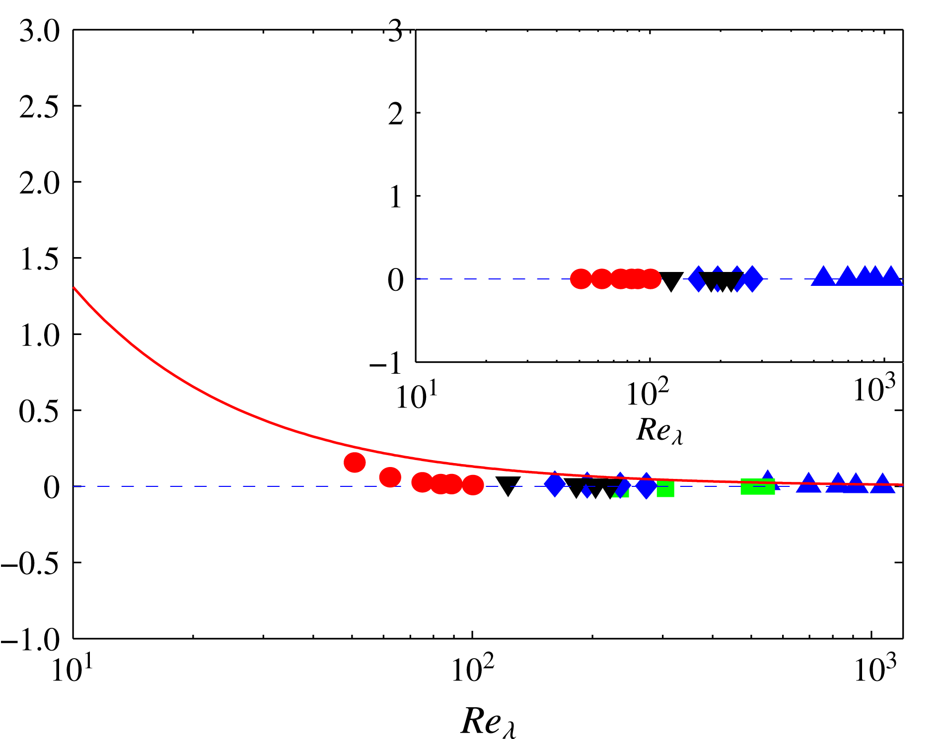
Dependence of
 $\unicode[STIX]{x1D6FD}_{2}\overline{(\unicode[STIX]{x2202}^{3}u^{\ast }/\unicode[STIX]{x2202}x^{\ast 3})(\unicode[STIX]{x2202}u^{\ast }/\unicode[STIX]{x2202}x^{\ast })^{2}}$
(symbols) on
 $Re_{\unicode[STIX]{x1D706}}$
in various flows: grid turbulence, ● (Zhou & Antonia Reference Zhou and Antonia2000); wakes, ♦ and ▾ correspond to data in wakes generated by two different initial conditions, namely a solid circular cylinder and a screen strip (Antonia, Zhou & Romano Reference Antonia, Zhou and Romano2002); circular jet centreline, ▪ (Xu, Antonia & Rajagopalan Reference Xu, Antonia and Rajagopalan2001); plane jet, ▴ (Zhou, Antonia & Chua Reference Zhou, Antonia and Chua2005). The inset shows the magnitude of
 $\unicode[STIX]{x1D6FD}_{3}\overline{(\unicode[STIX]{x2202}^{3}u^{\ast }/\unicode[STIX]{x2202}x^{\ast 3})(\unicode[STIX]{x2202}u^{\ast }/\unicode[STIX]{x2202}y^{\ast })^{2}}$
. Also shown is the large-scale term (red curve, right-hand side of (2.16)) (
 $n=1.2$
). The blue dashed line corresponds to the value of 0.
For convenience, we have replaced
 $\unicode[STIX]{x1D6FD}_{4}$
by
 $\unicode[STIX]{x1D6FD}$
. Equation (2.15) provides important insight into the physical mechanisms that affect the magnitude of the velocity derivative flatness factor
 $S_{4}$
: (i) The term on the right, which represents the large-scale contribution, contains
 $S_{3}$
, since it stems from term 1 in (2.1). It can be interpreted as the rate of change of the skewness (or rate of vortex stretching). (ii) The second term on the left represents the pressure diffusion while the third and fourth terms represent viscous destruction. The magnitude of
 $S_{4}$
can be considered to be controlled by the balance between the decay and/or production of the skewness, the pressure diffusion of energy (the second term on the left of (2.15)) and viscous/destructive effects (the third and fourth terms on the left of (2.15)). Figure 1 shows the dependence of the viscous/destructive effect term
 $\unicode[STIX]{x1D6FD}_{2}\overline{(\unicode[STIX]{x2202}^{3}u^{\ast }/\unicode[STIX]{x2202}x^{\ast 3})(\unicode[STIX]{x2202}u^{\ast }/\unicode[STIX]{x2202}x^{\ast })^{2}}$
(symbols) on
 $Re_{\unicode[STIX]{x1D706}}$
in various flows; the inset shows the viscous/destructive term
 $\unicode[STIX]{x1D6FD}_{3}\overline{(\unicode[STIX]{x2202}^{3}u^{\ast }/\unicode[STIX]{x2202}x^{\ast 3})(\unicode[STIX]{x2202}u^{\ast }/\unicode[STIX]{x2202}y^{\ast })^{2}}$
. Also shown in figure 1 is the large-scale term (red curve) with
 $n=1.2$
. It can be seen that the viscous/destructive effect terms approach zero quickly whereas the large-scale term deceases gradually as
 $Re_{\unicode[STIX]{x1D706}}$
increases. Namely, the contribution of the viscous/destructive term is negligible at relatively small
 $Re_{\unicode[STIX]{x1D706}}$
. To our knowledge, no DNS estimates for the pressure-diffusion term in (2.15) are available. Application of the Cauchy–Schwarz theorem to this term yields
 $$\begin{eqnarray}\left|\overline{\left(\frac{\unicode[STIX]{x2202}u}{\unicode[STIX]{x2202}x}\right)^{2}\frac{\unicode[STIX]{x2202}^{2}p}{\unicode[STIX]{x2202}x^{2}}}\right|\leqslant \overline{\left(\frac{\unicode[STIX]{x2202}u}{\unicode[STIX]{x2202}x}\right)^{4}}^{1/2}\overline{\left(\frac{\unicode[STIX]{x2202}^{2}p}{\unicode[STIX]{x2202}x^{2}}\right)^{2}}^{1/2},\end{eqnarray}$$
which finally leads to
 $$\begin{eqnarray}\left|\overline{\left(\frac{\unicode[STIX]{x2202}u^{\ast }}{\unicode[STIX]{x2202}x^{\ast }}\right)^{2}\left(\frac{\unicode[STIX]{x2202}^{2}p^{\ast }}{\unicode[STIX]{x2202}x^{\ast 2}}\right)}\right|\leqslant S_{4}^{1/2}\left(\int _{0}^{\infty }k^{\ast 4}E_{p}^{\ast }(k^{\ast })\,\text{d}k^{\ast }\right)^{1/2},\end{eqnarray}$$
where
 $E_{p}(k)$
is the three-dimensional pressure spectrum. Therefore, when
 $Re_{\unicode[STIX]{x1D706}}$
is sufficiently large (the viscous/destructive and large-scale terms will become negligible), equation (2.16) can be written as
 $$\begin{eqnarray}S_{4}\approx \left|\unicode[STIX]{x1D6FD}_{1}\overline{\left(\frac{\unicode[STIX]{x2202}u^{\ast }}{\unicode[STIX]{x2202}x^{\ast }}\right)^{2}\left(\frac{\unicode[STIX]{x2202}^{2}p^{\ast }}{\unicode[STIX]{x2202}x^{\ast 2}}\right)}\right|\leqslant \unicode[STIX]{x1D6FD}_{1}S_{4}^{1/2}\left(\int _{0}^{\infty }k^{\ast 4}E_{p}^{\ast }(k^{\ast })\,\text{d}k^{\ast }\right)^{1/2}\end{eqnarray}$$
or
 $$\begin{eqnarray}S_{4}^{1/2}\leqslant \left(\int _{0}^{\infty }k^{\ast 4}E_{p}^{\ast }(k^{\ast })\,\text{d}k^{\ast }\right)^{1/2}.\end{eqnarray}$$
Djenidi et al. (Reference Djenidi, Antonia, Danaila and Tang2017b
) inferred, on the basis of the DNS results of Ishihara et al. (Reference Ishihara, Kaneda, Yokokawa, Itakura and Uno2003), that this integral tends to a constant for sufficiently large Reynolds numbers, implying that
 $S_{4}$
should be bounded when
 $Re_{\unicode[STIX]{x1D706}}$
is sufficiently large. An increased rate of local vortex stretching leads to an increased concentration of turbulent fluctuations in reduced regions of space, and hence an increased intermittency and larger skewness and flatness factors. The pressure diffusion term accounts for non-local interactions. It represents the correlation between the fluctuating local energy dissipation rate and one component of the Laplacian of the pressure fluctuation. The physical interpretation of (1.4) is now well understood: viscous effects act to limit the final value of
 $S_{3}$
once
 $Re_{\unicode[STIX]{x1D706}}$
is sufficiently large (i.e. when
 $C/Re_{\unicode[STIX]{x1D706}}$
is negligible). One can similarly argue that the flatness factor
 $S_{4}$
, as given by (2.15), is expected to become constant when
 $Re_{\unicode[STIX]{x1D706}}$
is sufficiently large, i.e. the enhancement of ‘intermittency’ must be halted by the effect of both pressure diffusion and viscous terms on the left-hand side of (2.15). As the Reynolds number increases, the decay and/or production of the skewness as well as the viscous destruction decrease gradually before disappearing altogether, leaving only the pressure diffusion to balance
 $S_{4}$
. Gotoh & Nakano (Reference Gotoh and Nakano2003) discussed the role of the pressure diffusion by examining the transport equation for
 $S_{n}$
(
 $n=4$
, 6 and 8) using DNS data. They proposed a model for the pressure diffusion, based on Bernoulli’s equation, and argued that the pressure gradient acts to resist vortex stretching, thus limiting the level of intermittency. We recall that Kraichnan (Reference Kraichnan1991) had pointed to the possibility that pressure forces can attenuate the intermittency, leading to universal statistics of dissipation range scales.
The interplay between the different physical mechanisms described above is conceptually analogous to the fact that the skewness of the derivative (again, for large Reynolds numbers) is only balanced by the viscous destruction of the second-order moments (or energy), as reflected by (1.4). Reasoning by ‘induction’ would lead to the expectation that the
 $n$
th-order moments of the velocity derivative are balanced mainly by the viscous destruction of the
 $(n-1)$
th-order moments. In § 3, we further examine the main outcome of this section, i.e. (2.15) or (2.16), using experimental data for
 $S_{4}$
; naturally, we recognize that (2.15) can only be tested realistically once reliable DNS estimates of the pressure-diffusion term become available.
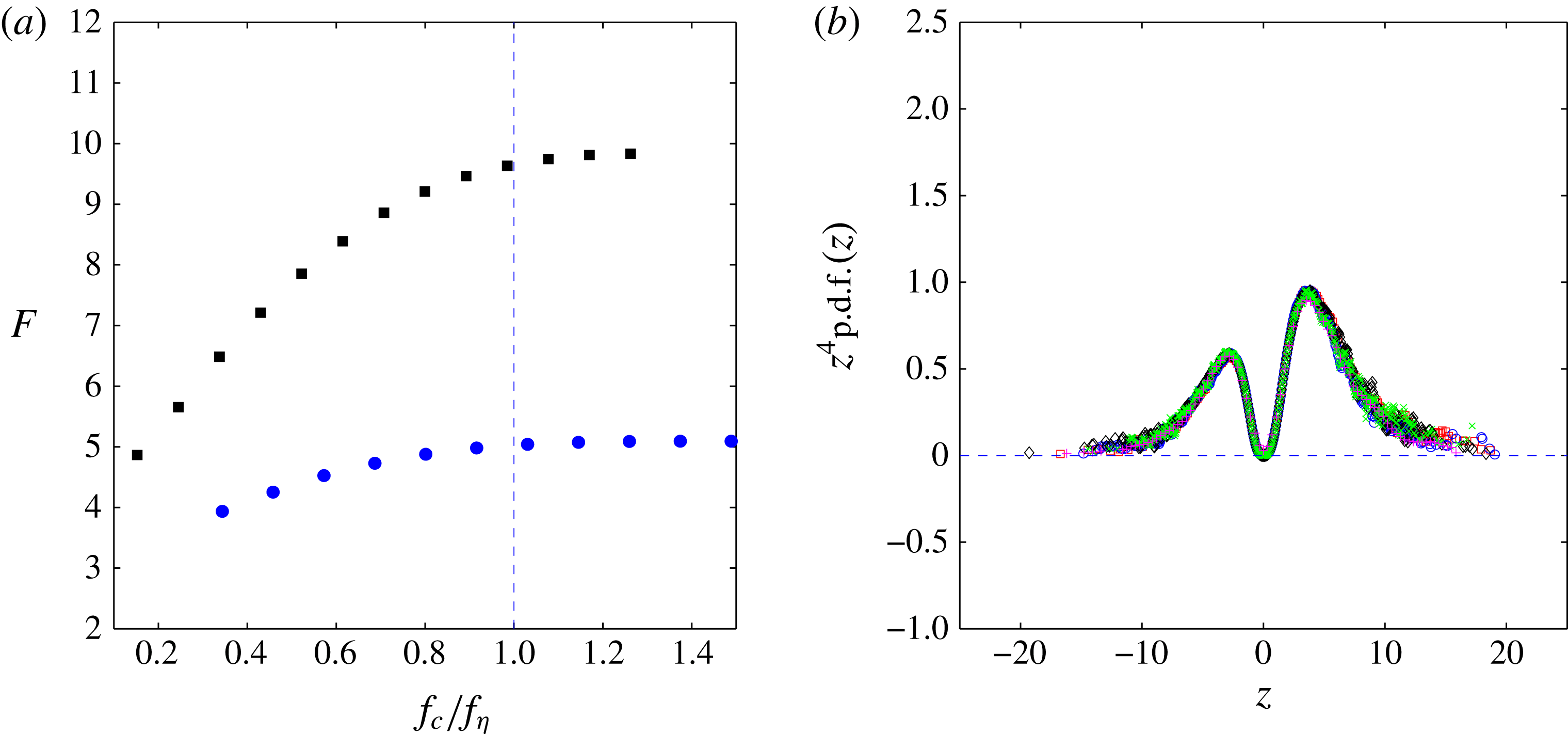
(a) Dependence of
 $F$
on
 $\mathit{f}_{c}/\mathit{f}_{\unicode[STIX]{x1D702}}$
for the plane jet data at
 $Re_{\unicode[STIX]{x1D706}}=550$
(▪; Zhou et al.
Reference Zhou, Antonia and Chua2005) and the channel flow data at
 $Re_{\unicode[STIX]{x1D706}}=36$
(●; Tang et al.
Reference Tang, Antonia, Djenidi, Abe, Zhou, Danaila and Zhou2015a
). The vertical dashed line corresponds to
 $\mathit{f}_{c}/\mathit{f}_{\unicode[STIX]{x1D702}}=1$
. (b) The probability density function (p.d.f.) of
 $z$
multiplied by
 $z^{4}$
along the axis of the plane jet with
 $Re_{\unicode[STIX]{x1D706}}=550$
(black), 696 (blue), 826 (red), 914 (pink) and 1067 (green) (Zhou et al.
Reference Zhou, Antonia and Chua2005). The dashed line indicates the value of 0.
3 Results for
 $S_{4}$

3.1 Measurement of
$S_{4}$

Difficulties in measuring small-scale quantities such as
 $S_{4}$
(often denoted by
 $F$
in the literature; we will hereafter use
 $F$
and
 $S_{4}$
interchangeably) have been discussed in detail by Antonia et al. (Reference Antonia, Satyaprakash and Hussain1982). Therefore, before discussing the results, it is important to comment on the accuracy of the measurements of
 $F$
(Zhou & Antonia Reference Zhou and Antonia2000; Pearson & Antonia Reference Pearson and Antonia2001; Antonia et al.
Reference Antonia, Zhou and Romano2002; Zhou et al.
Reference Zhou, Antonia and Chua2005; Tang et al.
Reference Tang, Antonia, Djenidi, Abe, Zhou, Danaila and Zhou2015a
) that are used here. There are three major ‘systematic’ error sources when measuring
 $F$
: the uncertainty associated with the spatial/time resolutions of the hot wire, and the duration of the recorded signal. As an example, for the plane jet data, the spatial resolution of the wire is adequate even at the largest
 $Re_{\unicode[STIX]{x1D706}}$
(
 $=1109$
; Pearson & Antonia Reference Pearson and Antonia2001) due to the fact that the wire diameter is
 $1.27~\unicode[STIX]{x03BC}\text{m}$
(the wire length is
 ${\sim}3.1\unicode[STIX]{x1D702}$
). In fact, for a single hot-wire measurement, the magnitude of
 $F$
is mainly affected by the temporal resolution and is practically insensitive to the spatial resolution (Burattini, Lavoie & Antonia (Reference Burattini, Lavoie and Antonia2008) demonstrated this in the context of
 $S_{3}$
). Figure 2(a) shows that the magnitude of
 $F$
increases with
 $\mathit{f}_{c}/\mathit{f}_{\unicode[STIX]{x1D702}}$
(
 $\mathit{f}_{c}$
and
 $\mathit{f}_{\unicode[STIX]{x1D702}}=U/2\unicode[STIX]{x03C0}\unicode[STIX]{x1D702}$
are the filter cutoff frequency and the Kolmogorov frequency, respectively), approximately reaches a maximum at
 $\mathit{f}_{c}/\mathit{f}_{\unicode[STIX]{x1D702}}\approx 1.0$
and remains constant at higher frequencies. For most of our data,
 $\mathit{f}_{c}$
was chosen close to or slightly larger than the Kolmogorov frequency
 $\mathit{f}_{\unicode[STIX]{x1D702}}$
(i.e.
 $\mathit{f}_{c}/\mathit{f}_{\unicode[STIX]{x1D702}}\geqslant 1$
), which is adequate for estimating
 $F$
(see figure 2
a). The final choice of
 $f_{c}$
was dictated by the onset of the electronic noise in the anemometer circuit. The record duration is also adequate since both
 $z^{2}\,\text{p.d.f.}(z)$
and
 $z^{4}\,\text{p.d.f.}(z)$
go to zero at large
 $|z|$
(figure 2
b). There remains the possibility of a random error associated mainly with the propagation of errors due mostly to the measurement of
 $u$
. An estimate was obtained from three single wires in the vorticity probe and shown as error bars in figures 3 and 4 for the data of Antonia et al. (Reference Antonia, Zhou and Romano2002) and Zhou et al. (Reference Zhou, Antonia and Chua2005).
Distributions of
 $F$
for various flows at relatively low
 $Re_{\unicode[STIX]{x1D706}}$
. Centreline of a fully developed channel flow: ▫, estimated from the data of Tang et al. (Reference Tang, Antonia, Djenidi, Abe, Zhou, Danaila and Zhou2015a
). SFPBT:
 $\times$
, Kerr (Reference Kerr1985). Grid turbulence: ▵, estimated from the data of Zhou & Antonia (Reference Zhou and Antonia2000). Wakes: ○ and ▿ correspond to data in wakes generated by two different initial conditions, namely a solid circular cylinder and a screen strip, estimated from the data of Antonia et al. (Reference Antonia, Zhou and Romano2002). The error bars for wake data are also shown; note that they are very small. To facilitate visual comparison with data in other flows, the ordinate scale used in this figure is the same as that in figures 4, 5, 6, 7 and 8(b).

3.2 Velocity derivative flatness
$F$
at relatively small
$Re_{\unicode[STIX]{x1D706}}$


Antonia et al. (Reference Antonia, Tang, Djenidi and Danaila2015) showed that, although
 $S_{3}$
approaches a constant when
 $Re_{\unicode[STIX]{x1D706}}$
is sufficiently large, the magnitude of
 $S_{3}$
is flow-dependent when
 $Re_{\unicode[STIX]{x1D706}}$
is small or moderate. There is no a priori reason why
 $S_{4}$
should behave differently than
 $S_{3}$
when
 $Re_{\unicode[STIX]{x1D706}}$
varies. The similarity between (1.4) and (2.16) suggests that
 $S_{4}$
should also depend on the type of flow at small to moderate
 $Re_{\unicode[STIX]{x1D706}}$
. To verify this, we report (figure 3) values of
 $F$
in various turbulent flows at relatively small
 $Re_{\unicode[STIX]{x1D706}}$
, e.g. grid turbulence, along the centreline of a fully developed channel flow, and ‘stationary’ forced periodic box turbulence (SFPBT) at relatively low
 $Re_{\unicode[STIX]{x1D706}}$
. In these flows, local isotropy (LI), which is a key ingredient of K41 and K62, is satisfied closely (see Antonia et al.
Reference Antonia, Tang, Djenidi and Danaila2015; Tang et al.
Reference Tang, Antonia, Djenidi, Abe, Zhou, Danaila and Zhou2015a
,Reference Tang, Antonia, Djenidi and Zhou
b
); along the axis in the far field of a plane jet, LI is also satisfied closely (Antonia et al.
Reference Antonia, Djenidi, Danaila and Tang2017). The data show a clear trend:
 $F$
increases as
 $Re_{\unicode[STIX]{x1D706}}$
increases for all the flows considered. The magnitude of
 $F$
is larger along the channel centreline than for either grid turbulence or SFPBT. Note that the distributions of
 $F$
obtained in two different grid turbulence experiments agree well over the same
 $Re_{\unicode[STIX]{x1D706}}$
range. Also included in figure 3 are the data in wakes generated by two different initial conditions: a solid circular cylinder and screen strip; they are estimated from the data of Antonia et al. (Reference Antonia, Zhou and Romano2002). Thiesset, Danaila & Antonia (Reference Thiesset, Danaila and Antonia2013) used the same wake data to assess LI through the isotropic relation between second-order structure functions of the lateral and longitudinal velocity increments, viz.
 $$\begin{eqnarray}\overline{(\unicode[STIX]{x1D6FF}v)^{2}}_{iso}=\left(1+\frac{r}{2}\frac{\text{d}}{\text{d}r}\right)\overline{(\unicode[STIX]{x1D6FF}u)^{2}}.\end{eqnarray}$$
They showed that (3.1) is satisfied in the dissipative range (
 $r^{\ast }<20$
), although the range of separations over which (3.1) is satisfied depends on the initial conditions. Figure 3, which shows that
 $F$
is multivalued, suggests that
 $F$
can, for a given flow, depend on the initial conditions. It can also vary from flow to flow.
Dependence of
 $F$
on
 $Re_{\unicode[STIX]{x1D706}}$
in two types of flows and qualitative comparison with (2.16). Plane jet:
 $\star$
, Antonia, Anselmet & Chambers (Reference Antonia, Anselmet and Chambers1986); ▾ (black), Sreenivasan & Antonia (Reference Sreenivasan and Antonia1997); ▪, Antonia et al. (Reference Antonia, Djenidi, Danaila and Tang2017), without identifying the data sources. Circular jet: ▵, Mi, Xu & Zhou (Reference Mi, Xu and Zhou2013); ♦, Xu et al. (Reference Xu, Antonia and Rajagopalan2001); ●, Kahalerras, Malecot & Gagne (Reference Kahalerras, Malecot and Gagne1998); ▾ (blue), Pearson & Antonia (Reference Pearson and Antonia2001); ▴, Friehe, Atta & Gibson (Reference Friehe, Van Atta and Gibson1971); ▿, Kuo & Corrsin (Reference Kuo and Corrsin1971); ▫, Antonia et al. (Reference Antonia, Chambers and Satyaprakash1981) (see also Antonia et al.
Reference Antonia, Satyaprakash and Hussain1982); ▹, Burattini (private communication). The blue and black curves are least-squares fits with (2.16), corresponding to circular jet (
 $\unicode[STIX]{x1D6FE}=-11$
and
 $\unicode[STIX]{x1D6FD}=1000$
) and plane jet (
 $\unicode[STIX]{x1D6FE}=-11$
and
 $\unicode[STIX]{x1D6FD}=1600$
), respectively. The inset shows all the data using log–log coordinates. Also shown in the inset is the K62 prediction (red curve):
 $F=0.91Re_{\unicode[STIX]{x1D706}}^{0.39}$
(Gylfason, Ayyalasomayajula & Warhaft Reference Gylfason, Ayyalasomayajula and Warhaft2004).

3.3 Derivative flatness factor
$S_{4}$
at large
$Re_{\unicode[STIX]{x1D706}}$


We now consider data for
 $S_{4}$
obtained by various authors in a wide range of flows. Separate plots are used (figures 4, 6, 7 and 8
b), with the same ordinate scale. We note that almost all the previous assessments of the
 $Re_{\unicode[STIX]{x1D706}}$
dependence of
 $F$
have included the high-
 $Re_{\unicode[STIX]{x1D706}}$
ASL data and led to the observation that
 $F\sim Re_{\unicode[STIX]{x1D706}}^{\unicode[STIX]{x1D6FC}_{4}}$
(K62), e.g. figure 6 of Sreenivasan & Antonia (Reference Sreenivasan and Antonia1997). For reasons that will be discussed in detail later (in the context of figure 8
a), we have excluded the ASL data from figures 4, 6, 7 and 8(b).
Recently, Antonia et al. (Reference Antonia, Djenidi, Danaila and Tang2017) showed that, along the axis of the far field of a plane jet,
 $F$
is practically constant over a range of
 $Re_{\unicode[STIX]{x1D706}}$
(
 $500<Re_{\unicode[STIX]{x1D706}}<1100$
) for several datasets, which are reproduced in figure 4 without identifying the data sources. Also included in figure 4 are the data of Antonia et al. (Reference Antonia, Anselmet and Chambers1986) and Sreenivasan & Antonia (Reference Sreenivasan and Antonia1997) also for the plane jet at lower
 $Re_{\unicode[STIX]{x1D706}}$
. In order to examine the boundedness of
 $F$
, we have added in figure 4 data obtained along the axis of the far field of a circular jet (Friehe et al.
Reference Friehe, Van Atta and Gibson1971; Kuo & Corrsin Reference Kuo and Corrsin1971; Antonia et al.
Reference Antonia, Chambers and Satyaprakash1981, Reference Antonia, Satyaprakash and Hussain1982; Kahalerras et al.
Reference Kahalerras, Malecot and Gagne1998; Pearson & Antonia Reference Pearson and Antonia2001; Xu et al.
Reference Xu, Antonia and Rajagopalan2001; Mi et al.
Reference Mi, Xu and Zhou2013). Antonia et al. (Reference Antonia, Satyaprakash and Hussain1982) measured
 $F$
on the centreline of a circular jet at
 $x/d=70$
, 80, 90 and 120 at a fixed
 $Re_{d}$
(
 $=U_{j}d/\unicode[STIX]{x1D708}=55\,600$
, where
 $U_{j}$
is the jet exit velocity and
 $d$
the nozzle diameter) on the jet axis (see their figure 7) and showed that
 $F$
is approximately constant (
 ${\approx}10$
) at
 $x/d=80$
, 90 and 120, respectively, which would be consistent with self-preservation at least for the small scales, and is also in good agreement with other data at comparable
 $Re_{\unicode[STIX]{x1D706}}$
in this flow (see figure 4). Their magnitude of
 $F$
at
 $x/d=70$
(
 ${\approx}8.4$
) appears to be underestimated, compared to
 $F$
for
 $x/d>70$
. For this reason, this data point is not shown in figure 4.
Equation (1.4) allows the FRN effect on
 $S_{3}$
to be estimated quantitatively in various flows, i.e. it allows an analytical prediction for
 $S_{3}$
. Evidently, it would be desirable to investigate the FRN effect on
 $F$
with (2.16) in each flow. However, the estimation of
 $\unicode[STIX]{x1D6FE}$
involves the simultaneous measurement of pressure and velocity fluctuations. Unfortunately, these quantities are not yet available and we only know the constant for
 $\unicode[STIX]{x1D6FD}$
in decaying HIT. Thus, we cannot predict
 $F$
analytically. However, in order to highlight the
 $Re_{\unicode[STIX]{x1D706}}$
dependence of
 $F$
, we apply a least-squares fit based on (2.16) to the data reported in figure 4; we assume that
 $\unicode[STIX]{x1D6FE}$
and
 $\unicode[STIX]{x1D6FD}$
are constants with the expectation that
 $\unicode[STIX]{x1D6FD}$
should vary between different flows to reflect the difference of FRN effect in each flow. As mentioned in the introduction,
 $S_{3}$
appears to reach the same constant value (
 ${\approx}-0.53$
) when
 $Re_{\unicode[STIX]{x1D706}}\geqslant 300$
; further, for
 $Re_{\unicode[STIX]{x1D706}}$
in the range 100–300,
 $S_{3}$
changes by less than 20 % in different flows (Antonia et al.
Reference Antonia, Djenidi, Danaila and Tang2017). We have therefore chosen
 $S_{3}\approx -0.53$
for curve fitting to these two flows. The fitted curves are shown in figure 4. The following comments can be made.
(i) The data in these two flows can be reasonably fitted with (2.16), with the same value of
$\unicode[STIX]{x1D6FE}~(=-11)$
but different values of
$\unicode[STIX]{x1D6FD}$
(1000 for the circular jet and 1600 for the plane jet, respectively).(ii) The fitted curves show the same trend as the data: the flow dependence when
$Re_{\unicode[STIX]{x1D706}}$
is small to moderate (
${<}600$
) becomes smaller when
$Re_{\unicode[STIX]{x1D706}}\geqslant 600$
.(iii) The trend shown by the data and the curves is clear:
$F$
appears to approach a limiting value, possibly slightly smaller than 12, when
$Re_{\unicode[STIX]{x1D706}}$
is sufficiently large. In general,
$Re_{\unicode[STIX]{x1D706}}$
needs to exceed approximately 500 for
$F$
to be considered constant in these two flows. The way this constant is approached is flow-dependent.(iv) The larger
$\unicode[STIX]{x1D6FD}$
, the slower the rate at which the final value is reached. Evidently, the approach is slower on the axis of the plane jet (
$\unicode[STIX]{x1D6FD}=1600$
) than on the axis of the circular jet (
$\unicode[STIX]{x1D6FD}=1000$
).


The constancy of
 $F$
at large
 $Re_{\unicode[STIX]{x1D706}}$
is consistent with the analytical prediction of Qian (Reference Qian1986), who used a closure theory, the analytical results of Djenidi et al. (Reference Djenidi, Antonia, Danaila and Tang2017b
) and the prediction of K41. But it cannot be reconciled with K62, which predicts
 $F\sim Re_{\unicode[STIX]{x1D706}}^{\unicode[STIX]{x1D6FC}_{4}}$
. This can be observed clearly from the inset of figure 4, which shows that K62 (as an example, we show a K62 prediction (red curve):
 $F=0.91Re_{\unicode[STIX]{x1D706}}^{0.39}$
of Gylfason et al. (Reference Gylfason, Ayyalasomayajula and Warhaft2004)) is not supported by the experimental data in both circular and plane jets. In fact, the K62 prediction is at best tangential to the plane jet data and does not represent at all the circular jet data. Since FRN-affected data (collected in different flows) as well as the ASL data (possibly also affected by the FRN effect) were included in almost all the previous examinations of
 $F$
versus
 $Re_{\unicode[STIX]{x1D706}}$
, it is not surprising that a consensus has not been reached for the value of
 $\unicode[STIX]{x1D6FC}_{4}$
. Indeed, the exponent
 $\unicode[STIX]{x1D6FC}_{4}$
can vary between 0.31 and 0.41 (e.g. Van Atta & Antonia Reference Van Atta and Antonia1980; Antonia et al.
Reference Antonia, Satyaprakash and Hussain1982; Ishihara et al.
Reference Ishihara, Kaneda, Yokokawa, Itakura and Uno2007), depending on the intermittency models. The previous discussion leads to the conclusion that the difference in the values of
 $\unicode[STIX]{x1D6FC}_{4}$
reflects the difference in the way
 $F$
is affected by the different large-scale motions.
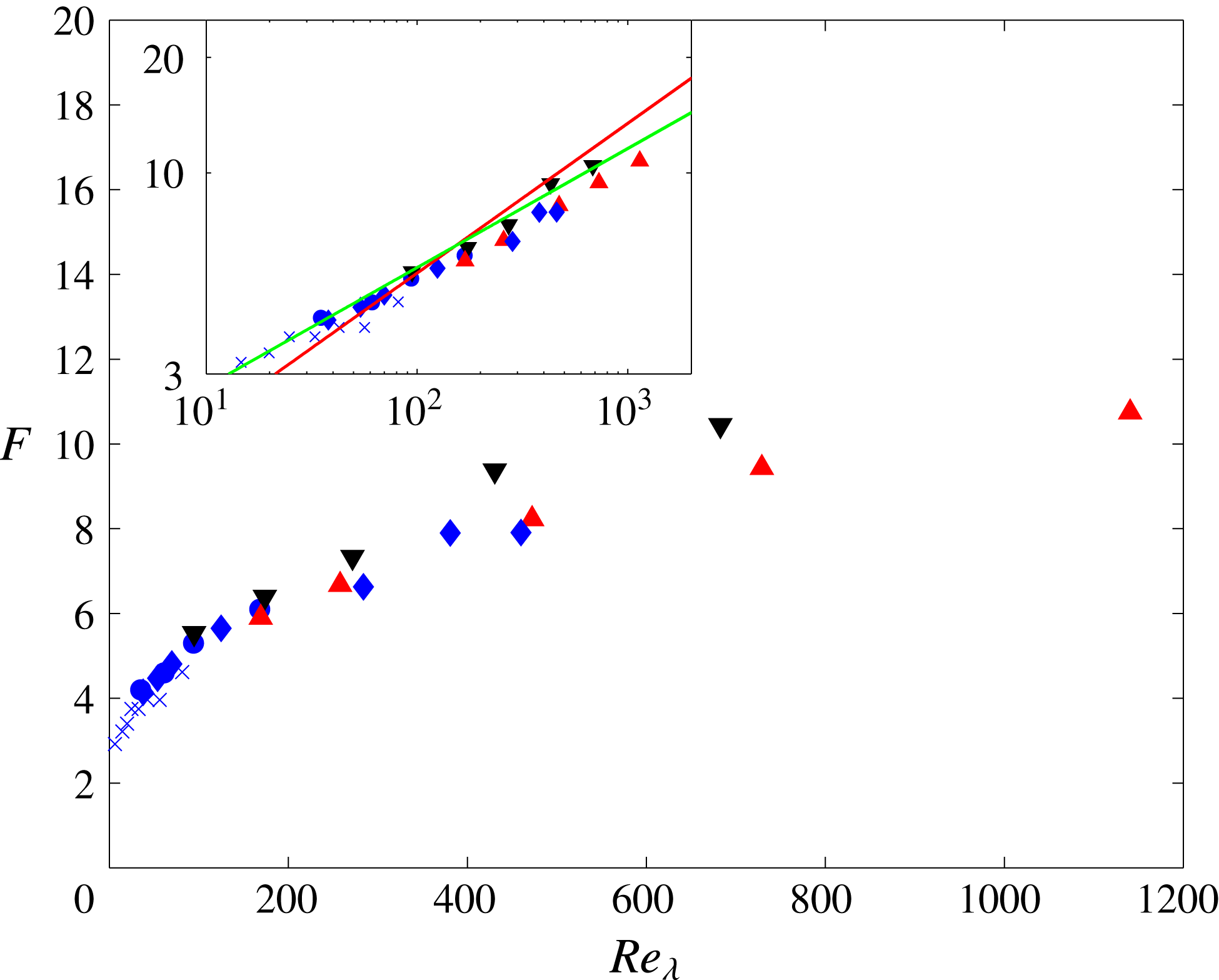
The DNS data for
 $F$
in SFPBT are shown figure 5. It can be seen from this figure that there is good collapse for all the DNS data when
 $Re_{\unicode[STIX]{x1D706}}\leqslant 200$
; the same can be observed for
 $S_{3}$
in the same flow; see figure 5 of Antonia et al. (Reference Antonia, Tang, Djenidi and Danaila2015). For
 $Re_{\unicode[STIX]{x1D706}}>200$
, however, the two sets of data obtained by Ishihara et al. (Reference Ishihara, Kaneda, Yokokawa, Itakura and Uno2007) (
 $k_{max}^{\ast }=2$
and
 $k_{max}^{\ast }=1$
, respectively) indicate that
 $F$
increases as
 $Re_{\unicode[STIX]{x1D706}}$
increases (the Gotoh et al. (Reference Gotoh, Fukayama and Nakano2002) data, for
 $k_{max}^{\ast }=1$
, give the impression that
 $F$
has almost become constant at
 $Re_{\unicode[STIX]{x1D706}}=460$
). The authors claim agreement with
 $F\sim Re_{\unicode[STIX]{x1D706}}^{\unicode[STIX]{x1D6FC}_{4}}$
(
 $\unicode[STIX]{x1D6FC}_{4}=0.31$
(Hill Reference Hill2002) and 0.39 (Gylfason et al.
Reference Gylfason, Ayyalasomayajula and Warhaft2004), respectively, which have also been shown in the inset of figure 5), but in fact it is clear that the rate of increase of
 $F$
with
 $Re_{\unicode[STIX]{x1D706}}$
decreases as
 $Re_{\unicode[STIX]{x1D706}}$
increases (see the linear plot) and the relation
 $F\sim Re_{\unicode[STIX]{x1D706}}^{\unicode[STIX]{x1D6FC}_{4}}$
does not really represent the trend of the Ishihara et al. (Reference Ishihara, Kaneda, Yokokawa, Itakura and Uno2007) data (see the log–log plot). We can only surmise that Ishihara et al.’s (Reference Ishihara, Kaneda, Yokokawa, Itakura and Uno2007) claim that
 $F\sim Re_{\unicode[STIX]{x1D706}}^{\unicode[STIX]{x1D6FC}_{4}}$
was influenced by the inclusion of the ASL data. We contend that their data do not exclude the possibility that it will approach a constant at large
 $Re_{\unicode[STIX]{x1D706}}$
. We have already commented (Antonia et al.
Reference Antonia, Tang, Djenidi and Danaila2015) on the behaviour of their Kolmogorov-normalized spectra, in particular the systematic increase of
 $k^{\ast 4}E^{\ast }(k^{\ast })$
(for
 $k^{\ast }>0.5$
) with
 $Re_{\unicode[STIX]{x1D706}}$
(Ishihara et al.
Reference Ishihara, Kaneda, Yokokawa, Itakura and Uno2007). This is not consistent with Kolmogorov scaling, as inferred from the NS equation (e.g. Antonia et al.
Reference Antonia, Djenidi and Danaila2014), nor is it consistent with the support for this scaling provided by previous DNS studies of forced periodic box turbulence (Jimenez et al.
Reference Jimenez, Wray, Saffman and Rogallo1993; Yeung & Zhou Reference Yeung and Zhou1997; Gotoh et al.
Reference Gotoh, Fukayama and Nakano2002; Yeung et al.
Reference Yeung, Donzis and Sreenivasan2005), for
 $Re_{\unicode[STIX]{x1D706}}$
up to 700. As overwhelmingly supported by experimental data – and also the DNS data of Jimenez et al. (Reference Jimenez, Wray, Saffman and Rogallo1993), Yeung & Zhou (Reference Yeung and Zhou1997), Gotoh et al. (Reference Gotoh, Fukayama and Nakano2002, see figure 12 of their paper) and Yeung et al. (Reference Yeung, Donzis and Sreenivasan2005, up to
 $Re_{\unicode[STIX]{x1D706}}\approx 700$
, see figure 1 of their paper) (note that
 $S_{3}$
is constant for
 $Re_{\unicode[STIX]{x1D706}}\approx 240{-}700$
whereas a proper ‘
 $4/5$
’ inertial range has yet to be established) – the FRN effect first disappears at the smallest scales and subsequently at increasingly larger scales as
 $Re_{\unicode[STIX]{x1D706}}$
increases. This is in contrast to the claim by Ishihara et al. (Reference Ishihara, Kaneda, Yokokawa, Itakura and Uno2007, Reference Ishihara, Gotoh and Kaneda2009) that the Reynolds-number effect has ‘nearly’ disappeared in the so-called scaling range (in Ishihara et al. (Reference Ishihara, Gotoh and Kaneda2009), the scaling range exponents, which are independent of
 $Re_{\unicode[STIX]{x1D706}}$
, are inferred from Gotoh et al.’s (Reference Gotoh, Fukayama and Nakano2002) data at
 $Re_{\unicode[STIX]{x1D706}}=460$
) whereas
 $S_{3}$
and
 $S_{4}$
continue to increase. Further, Ishihara et al. (Reference Ishihara, Gotoh and Kaneda2009) conclude (their summary point number 3) that
[t]he DNS data support the existence of a universal local equilibrium state at small scales in high
 $Re$
in the manner of K41
and (their summary point number 5) that
[…] with regard to the
 $Re$
dependences of statistics, (i) some statistics such as the energy-dissipation rate, the normalized third-order structure function, and the energy-flux spectrum in the inertial subrange tend toward finite constants as
 $Re\rightarrow \infty$
; (ii) others, such as the energy spectrum in the dissipation range, tend toward a form independent of
 $Re$
in accordance with K41, but the approach may be very slow; and (iii) some statistics, such as the skewness and flatness factors of the velocity gradients and pressure gradients, have an algebraic dependence on
 $Re_{\unicode[STIX]{x1D706}}$
.
These conclusions imply that K41 and K62 may coexist, a possibility that is difficult to understand, at least in the context of the laboratory measurements and previous and earlier DNS results. Our observations indicate that the FRN effect first disappears in the dissipative range and lingers on in the scaling range, i.e. larger scales (in the scaling range) are more likely to continue to be affected by
 $Re_{\unicode[STIX]{x1D706}}$
than smaller scales (in the dissipative range). Evidently, Ishihara et al. (Reference Ishihara, Kaneda, Yokokawa, Itakura and Uno2007) do not share this view. To our knowledge, a plausible mechanism, which explains how intermittency, as expressed by
 $F$
say, can continue to increase with
 $Re_{\unicode[STIX]{x1D706}}$
whilst the scaling range exponents are no longer affected by
 $Re_{\unicode[STIX]{x1D706}}$
(Ishihara et al.
Reference Ishihara, Gotoh and Kaneda2009), has yet to be proposed.
Dependence of
 $F$
on
 $Re_{\unicode[STIX]{x1D706}}$
in SFPBT:
 $\times$
, Kerr (Reference Kerr1985); ▾ and ▴ correspond to
 $k_{max}^{\ast }=2$
and
 $k_{max}^{\ast }=1$
, respectively, from Ishihara et al. (Reference Ishihara, Kaneda, Yokokawa, Itakura and Uno2007); ♦, Gotoh et al. (Reference Gotoh, Fukayama and Nakano2002); ●, Wang et al. (Reference Wang, Chen, Brasseur and Wyngaard1996). The inset shows all the data using log–log coordinates. Also shown in the inset is the K62 prediction:
 $F=0.91Re_{\unicode[STIX]{x1D706}}^{0.39}$
(red curve) (Gylfason et al.
Reference Gylfason, Ayyalasomayajula and Warhaft2004) and
 $F=1.36Re_{\unicode[STIX]{x1D706}}^{0.31}$
(green curve) (Hill Reference Hill2002); both predictions were used by Ishihara et al. (Reference Ishihara, Kaneda, Yokokawa, Itakura and Uno2007) (see their figure 6).
Dependence of
 $F$
on
 $Re_{\unicode[STIX]{x1D706}}$
in flow between counter-rotating disks: ○, Tabeling et al. (Reference Tabeling, Zocchi, Belin, Maurer and Willaime1996); ▫, Belin et al. (Reference Belin, Maurer, Tabeling and Willaime1997).
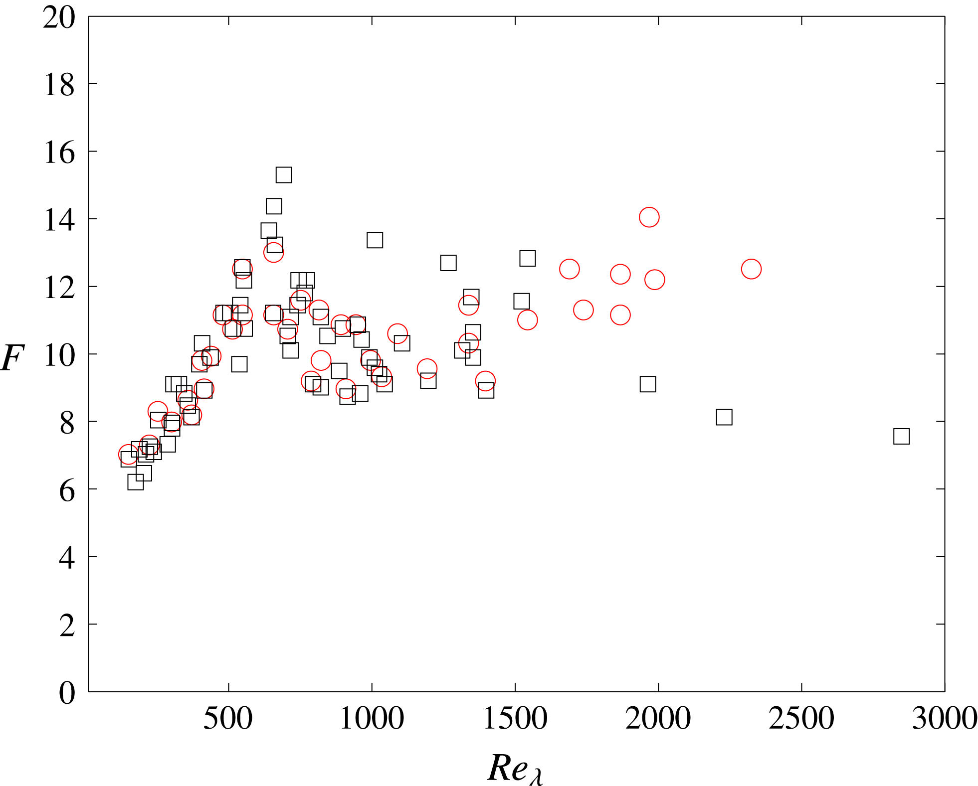
Tabeling et al. (Reference Tabeling, Zocchi, Belin, Maurer and Willaime1996) and Belin et al. (Reference Belin, Maurer, Tabeling and Willaime1997) reported various statistics for
 $\unicode[STIX]{x2202}u/\unicode[STIX]{x2202}x$
in helium gas at low temperature in a cylindrical container bounded by two counter-rotating disks over an impressively large range of
 $Re_{\unicode[STIX]{x1D706}}$
: 150–5040 (Tabeling et al.
Reference Tabeling, Zocchi, Belin, Maurer and Willaime1996) and 150–2300 (Belin et al.
Reference Belin, Maurer, Tabeling and Willaime1997). In the context of this paper, notwithstanding previous reservations (Sreenivasan Reference Sreenivasan1995; Sreenivasan & Antonia Reference Sreenivasan and Antonia1997) concerning the characteristics of the sensor used in these experiments, these results are useful since the range of
 $Re_{\unicode[STIX]{x1D706}}$
is large enough to allow the assessment of the FRN effect on
 $F$
with minimal ambiguity. As far as we are aware, there has been no systematic examination of LI in the central region of this flow. However, the isotropic form of the transport equation for
 $\overline{(\unicode[STIX]{x1D6FF}u)^{2}}$
is verified reasonably well (Moisy, Tabeling & Willaime Reference Moisy, Tabeling and Willaime1999). Antonia et al. (Reference Antonia, Tang, Djenidi and Danaila2015) have already reported and discussed elsewhere the data for
 $S_{3}$
, where
 $S_{3}$
remains constant (
 $\simeq -0.50$
) over a range of
 $Re_{\unicode[STIX]{x1D706}}$
extending up to 2000. The data for
 $F$
of Tabeling et al. (Reference Tabeling, Zocchi, Belin, Maurer and Willaime1996) and Belin et al. (Reference Belin, Maurer, Tabeling and Willaime1997) are shown in figure 6 for
 $Re_{\unicode[STIX]{x1D706}}$
up to 3000. The figure presents a similar trend to that of the data in figure 4:
 $F$
increases with
 $Re_{\unicode[STIX]{x1D706}}$
for
 $Re_{\unicode[STIX]{x1D706}}$
up to approximately 700, and, allowing for the scatter, seems to be approximately constant beyond that value. There is a peak in
 $F$
in the vicinity of
 $Re_{\unicode[STIX]{x1D706}}\simeq 700$
, which was speculated (by the authors) to correspond to a transition, possibly a ‘mixing’ transition as described by Dimotakis (Reference Dimotakis2000) and also observed by Pearson & Krogstad (Reference Pearson and Krogstad2001) in passive grid turbulence, to a new state of turbulence (see the discussion of this transition in Tabeling & Willaime (Reference Tabeling and Willaime2002)).
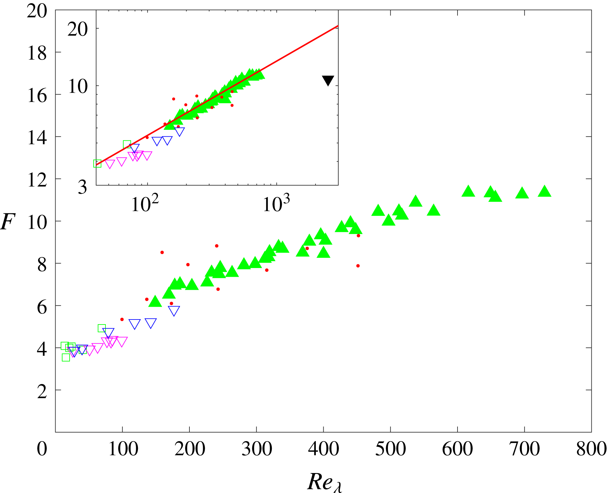
Dependence of
 $F$
on
 $Re_{\unicode[STIX]{x1D706}}$
in shearless grid turbulence: ▫, Batchelor & Townsend (Reference Batchelor and Townsend1947, Reference Batchelor and Townsend1949); ▿ (magenta), estimated from the data of Zhou & Antonia (Reference Zhou and Antonia2000) (
 $l_{w}/\unicode[STIX]{x1D702}=0.6{-}2.5$
); ▿ (blue), Tong & Warhaft (Reference Tong and Warhaft1994) (
 $l_{w}/\unicode[STIX]{x1D702}=0.8{-}1.3$
); ●, Mydlarski & Warhaft (Reference Mydlarski and Warhaft1996) (
 $l_{w}/\unicode[STIX]{x1D702}=1.8{-}5.2$
); ▴ corresponds to the data from small and large tunnels, respectively, without mean shear, reproduced from figure 3 of Gylfason et al. (Reference Gylfason, Ayyalasomayajula and Warhaft2004); note that only data for
 $l_{w}/\unicode[STIX]{x1D702}\leqslant 1.75$
are shown, as recommended by Gylfason et al. (Reference Gylfason, Ayyalasomayajula and Warhaft2004). The inset shows all the data on a log–log plot. Also shown in the inset is one measurement (
 $F=10.8$
, ▾) of Kahalerras et al. (Reference Kahalerras, Malecot and Gagne1998) along the axis of the ONERA wind tunnel (similar to grid turbulence) for
 $Re_{\unicode[STIX]{x1D706}}=2500$
and the K62 prediction (red curve):
 $F=0.91Re_{\unicode[STIX]{x1D706}}^{0.39}$
(Gylfason et al.
Reference Gylfason, Ayyalasomayajula and Warhaft2004).
Gylfason et al. (Reference Gylfason, Ayyalasomayajula and Warhaft2004) examined the Reynolds-number dependence of
 $F$
in grid turbulence with and without mean shear (
 $Re_{\unicode[STIX]{x1D706}}=100{-}1000$
). Here, we only show the data in grid turbulence without a mean shear since the latter has a significant effect on LI (Kim & Antonia Reference Kim and Antonia1993; Shen & Warhaft Reference Shen and Warhaft2000) (see also Tang et al. (Reference Tang, Antonia, Danaila, Djenidi, Zhou and Zhou2016), who showed that the higher-order statistics depart more strongly from LI in sheared than in shearless grid turbulence); not surprisingly, the magnitude of
 $F$
is increased, at the same
 $Re_{\unicode[STIX]{x1D706}}$
, relative to that measured without shear; also,
 $F$
increases along distinctly different paths for the shearless and sheared cases. Gylfason et al.’s (Reference Gylfason, Ayyalasomayajula and Warhaft2004) data (their figure 3) for shearless grid turbulence are reported in figure 7; note that only data for
 $l_{w}/\unicode[STIX]{x1D702}\leqslant 1.75$
are shown, as recommended by Gylfason et al. (Reference Gylfason, Ayyalasomayajula and Warhaft2004). Also shown in this figure are data for grid turbulence collected from other published studies. Two comments can be made with regard to figure 7.
(i) All the data for
$F$
collapse reasonably well onto a single distribution, up to
$Re_{\unicode[STIX]{x1D706}}\simeq 730$
. This distribution has the same behaviour as that observed in figure 4: for
$Re_{\unicode[STIX]{x1D706}}\leqslant$
600, the magnitude of
$F$
increases with
$Re_{\unicode[STIX]{x1D706}}$
; for
$Re_{\unicode[STIX]{x1D706}}\geqslant 600$
,
$F$
eventually reaches a constant, which is about the same as that measured by Kahalerras et al. (Reference Kahalerras, Malecot and Gagne1998) at
$Re_{\unicode[STIX]{x1D706}}=2500$
. This trend is similar to that observed in figures 4 and 6. On the contrary, the inset of figure 7 shows that shearless grid turbulence data (
$50<Re_{\unicode[STIX]{x1D706}}<160$
) from other published studies and especially the data point at
$Re_{\unicode[STIX]{x1D706}}=2500$
are not adequately described by the relation
$F=0.91Re_{\unicode[STIX]{x1D706}}^{0.39}$
(K62). Further, as discussed in the context of figures 4 and 5, Gylfason et al.’s relation
$F=0.91Re_{\unicode[STIX]{x1D706}}^{0.39}$
cannot represent the data in other flows.(ii) The data show that
$F$
approaches a constant whose magnitude is in approximate agreement with that in plane and circular jets when
$Re_{\unicode[STIX]{x1D706}}>600$
(figure 4).


(a) Dependence of
 $F$
on
 $Re_{\unicode[STIX]{x1D706}}$
reproduced (log–log plot) from figure 6 of Sreenivasan & Antonia (Reference Sreenivasan and Antonia1997) without identifying the data sources. A ‘red’ line has been drawn around the ASL data to distinguish these from the other (laboratory) data. (b) An enlargement of the range for (laboratory) data using linear axes. Note the presentation in (b) is completely consistent with that in figures 4–7.
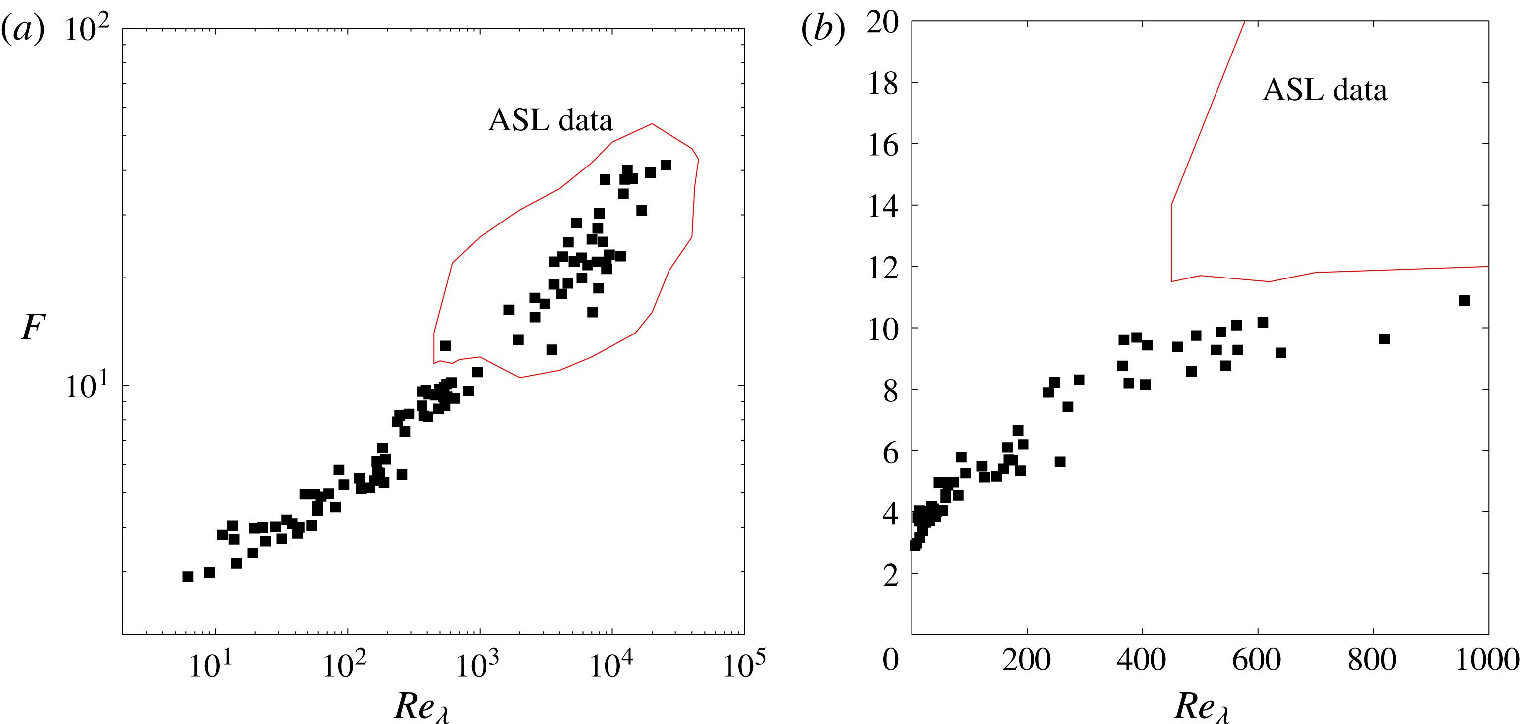
Figure 8(a) reproduces the compilation of
 $F$
versus
 $Re_{\unicode[STIX]{x1D706}}$
by Sreenivasan & Antonia (Reference Sreenivasan and Antonia1997) (their figure 6); we have drawn a ‘red’ line around the symbols corresponding to the ASL data. In order to compare figure 8(a) with figures 3–7, an enlargement of the
 $Re_{\unicode[STIX]{x1D706}}$
range corresponding to the laboratory data in figure 8(a) is shown in figure 8(b) with linear scales instead of log scales (the vertical scale is identical to that used in figures 4–7). Antonia et al. (Reference Antonia, Djenidi, Danaila and Tang2017) carried out a similar comparison for
 $S_{3}$
and made the following points.
(i) Since the data affected by the FRN effect were included in the compilation for
$S_{3}$
, many values of the exponent
$\unicode[STIX]{x1D6FC}_{3}$
in the power-law relation
$S_{3}\sim Re_{\unicode[STIX]{x1D706}}^{\unicode[STIX]{x1D6FC}_{3}}$
(K62) have been proposed.(ii) The ASL data should not be used to test K41 and K62 because they were collected at relatively small heights (often below 30 m) above the ground or ocean surface where the requirements for K41 and K62 are unlikely to be met. Similar comments can be made for
$F$
on the basis of figures 3–8.


It can be seen from figure 8(b) that there is a fair amount of ‘apparent’ scatter in the laboratory data for
 $Re_{\unicode[STIX]{x1D706}}\leqslant 600$
. In fact, this scatter reflects, to a large extent, the systematic difference in how
 $F$
approaches a constant in different flows, e.g. figure 3. In similar fashion to
 $S_{3}$
(Antonia et al.
Reference Antonia, Djenidi, Danaila and Tang2017), no attempt was made to distinguish between distributions of
 $F$
in different flows.
Almost all the previous examinations of
 $F$
versus
 $Re_{\unicode[STIX]{x1D706}}$
have included the high-
 $Re_{\unicode[STIX]{x1D706}}$
ASL data, e.g. figure 6 of Sreenivasan & Antonia (Reference Sreenivasan and Antonia1997) (or the present figure 8
a). The inclusion of the ASL data leads to a power-law dependence of
 $F$
on
 $Re_{\unicode[STIX]{x1D706}}$
(K62) that is inconsistent with the results in figures 4, 6 and 7. We have excluded the ASL data from figures 4, 6 and 7 since Djenidi et al. (Reference Djenidi, Antonia, Talluru and Abe2017c
) have provided several reasons why the ASL data should be discarded when testing K41 and K62. We discuss this further here, in some detail. The ASL data have been obtained in a flow region where the effects of the mean shear and proximity to the surface (which causes blockage effects to arise) cannot be ignored, notwithstanding the locally high value of
 $Re_{\unicode[STIX]{x1D706}}$
, especially since both these effects are known to induce strong departures from LI. In fact, a large percentage of the ASL data in figure 8(a) were obtained by Wyngaard & Tennekes (Reference Wyngaard and Tennekes1970) at three heights (
 $z=5.66$
, 11.3 and 22.6 m) above the ground (no information for the stability conditions is given). Under ‘neutral’ conditions, the ASL should be comparable (at similar values of
 $z/\unicode[STIX]{x1D6FF}$
) with the laboratory boundary layer provided the nature of the surface is comparable. It is difficult to estimate with confidence the thickness
 $\unicode[STIX]{x1D6FF}$
of the neutral ASL. Wyngaard (Reference Wyngaard2010) suggests that, under neutral conditions,
 $\unicode[STIX]{x1D6FF}$
may scale with
 $U_{\unicode[STIX]{x1D70F}}/f$
(
 $U_{\unicode[STIX]{x1D70F}}$
is the friction velocity and
 $f$
is the Coriolis parameter) and estimates, for mid-latitudes,
 $\unicode[STIX]{x1D6FF}$
to be within the range 250 to 2500 m. This implies that the majority of the neutral ASL data for
 $F$
were taken in the region
 $z/\unicode[STIX]{x1D6FF}<0.1$
. It is not difficult to conclude that there is quite a lot of uncertainty in the estimation of
 $\unicode[STIX]{x1D6FF}$
, e.g. a value of
 $\unicode[STIX]{x1D6FF}$
smaller than 100 m was found by Metzger, McKeon & Holmes (Reference Metzger, McKeon and Holmes2007) based on experiments in Utah’s western desert for almost ‘exactly’ neutral conditions; the authors stressed, however, the difficulties associated in making measurements under those conditions. In any case, it is not clear if any of the published ASL data were obtained under ‘exactly’ neutral conditions. Certainly, it is unwise to assume that the measurements of
 $F$
in region
 $z/\unicode[STIX]{x1D6FF}<0.1$
have not been affected by the proximity to the surface.
Recent measurements (Djenidi et al.
Reference Djenidi, Antonia, Talluru and Abe2017c
) in a laboratory boundary layer over smooth and rough walls indicate that the magnitude of
 $F$
can increase, perhaps by as much as a factor of 3, in the region
 $z/\unicode[STIX]{x1D6FF}<0.1$
. For the ASL data in figure 8(a) of Sreenivasan & Antonia (Reference Sreenivasan and Antonia1997), it is almost certain that
 $F$
was invariably estimated over a range of heights that would correspond to the inner region of the laboratory boundary layer. For example, for the nearly neutral ASL data measured by Gibson et al. (Reference Gibson, Stegen and Williams1970) above the ocean surface,
 $F$
is in the range 13 to 26 (the height is in the range 2.25 m to 12.25 m); this variation is typical of that found in the inner region of the laboratory boundary layer (Djenidi et al.
Reference Djenidi, Antonia, Talluru and Abe2017c
). Further, one should also check that there are no major departures from LI in this range due to the probable effect of the mean shear. In the region
 $z/\unicode[STIX]{x1D6FF}<0.1$
, a larger departure from LI is expected due to the combined effect of an increase in mean shear and the presence of the surface. Clearly, the use of
 $F$
in the first few metres of the ASL has misled a vast majority of researchers into preferring K62 over K41. More importantly, when the ASL data are disregarded, the (laboratory) data in figure 8(b) are consistent with the trend displayed in figures 4, 6 and 7, providing further strong support that
 $F$
increases as
 $Re_{\unicode[STIX]{x1D706}}$
increases, eventually becoming constant when
 $Re_{\unicode[STIX]{x1D706}}$
is sufficiently large. Note that the log–log scale in figure 8(a), together with the weighting of the ASL data, have ‘aided and abetted’ the support for a power-law dependence of
 $F$
on
 $Re_{\unicode[STIX]{x1D706}}$
.
4 Conclusions and final discussion
An analytical expression for the flatness factor
 $F$
in HIT has been derived by applying the limit at small separation to the transport equation for
 $\overline{(\unicode[STIX]{x1D6FF}u)^{3}}$
. The FRN effect, due to the influence of the large-scale motion, can be recast in the form
 $\unicode[STIX]{x1D6FD}S_{3}/Re_{\unicode[STIX]{x1D706}}$
(2.16). This is of similar form to the FRN effect on
 $S_{3}$
, i.e.
 $C/Re_{\unicode[STIX]{x1D706}}$
in (1.4). The analysis is developed solely by assuming local homogeneity and isotropy. The final expression for
 $F$
indicates that this quantity, which is often used as a measure of intermittency, is balanced mostly by the pressure diffusion of energy, viscous destructive effects and large-scale effects (decay and/or production). We have estimated that the viscous destructive effect is negligible at moderate values of
 $Re_{\unicode[STIX]{x1D706}}$
. Since the large-scale effect decreases as
 $Re_{\unicode[STIX]{x1D706}}^{-1}$
,
 $F$
is expected to be balanced solely by the correlation
 $\overline{(\unicode[STIX]{x2202}u^{\ast }/\unicode[STIX]{x2202}x^{\ast })^{2}(\unicode[STIX]{x2202}^{2}p^{\ast }/\unicode[STIX]{x2202}x^{\ast 2})}$
, thus emphasizing the role of the pressure fluctuation in limiting the growth of intermittency, as measured by
 $F$
. This correlation is expected to become constant at sufficiently large
 $Re_{\unicode[STIX]{x1D706}}$
. A possible physical interpretation of (2.15) is as follows. Enhanced local vortex stretching leads to an increased concentration of turbulent fluctuations in reduced regions of space. This results in an increased intermittency as reflected in the skewness and, more markedly, the flatness factor. The pressure diffusion term, which accounts for non-local interactions (reflected by the contributions of all wavenumbers to the integral in (2.18)), acts to slow down the rate at which the intermittency increases with
 $Re_{\unicode[STIX]{x1D706}}$
whilst viscous effects (through the term
 $G/Re_{\unicode[STIX]{x1D706}}$
in (1.4)) account for the destruction of the skewness
 $S_{3}$
. Speculatively it would appear that the pressure diffusion effect in (2.15) is not as effective as the viscous destruction term of
 $S_{3}$
so that
 $F$
tends to a constant at larger values of
 $Re_{\unicode[STIX]{x1D706}}$
than
 $S_{3}$
. DNS results for
 $\overline{(\unicode[STIX]{x2202}u^{\ast }/\unicode[STIX]{x2202}x^{\ast })^{2}(\unicode[STIX]{x2202}^{2}p^{\ast }/\unicode[STIX]{x2202}x^{\ast 2})}$
, in both forced turbulence and other turbulent flows, are needed to confirm this speculation.
The variation of
 $F$
with
 $Re_{\unicode[STIX]{x1D706}}$
has been examined in various turbulent flows: on the axis in the far field of plane and circular jets, grid turbulence, SFPBT, along the centreline of wakes, a fully developed channel flow, and the flow of helium gas at low temperature between two counter-rotating disks. In particular, we reinterpret this variation in the light of the FRN effect (Antonia et al.
Reference Antonia, Djenidi, Danaila and Tang2017). Figures 3 and 4 show clearly that, at relatively low
 $Re_{\unicode[STIX]{x1D706}}$
,
 $F$
can differ from flow to flow and, for a given flow, it may also depend on the initial conditions. This FRN effect on
 $F$
is further highlighted by applying least-square fits, using (2.16), to the circular jet and plane jet data (see figure 4); it strongly supports the notion that
 $F$
is affected by the FRN effect differently in different flows. The magnitude of
 $F$
in various flows (figures 4, 6 and 7), e.g. in grid turbulence, and along the axes in the far field of plane and circular jets, increases as
 $Re_{\unicode[STIX]{x1D706}}$
increases, and appears to approach a constant, with a value slightly larger than 10, when
 $Re_{\unicode[STIX]{x1D706}}$
is sufficiently large. This trend is consistent with all the laboratory data for
 $F$
examined by Sreenivasan & Antonia (Reference Sreenivasan and Antonia1997). More importantly, if we ignore the ASL data, all the laboratory data for
 $F$
seem consistent with K41, at least when
 $Re_{\unicode[STIX]{x1D706}}$
approaches
 $10^{3}$
, in the sense that
 $F$
approaches a constant value; this is also consistent with the analysis of § 2. It is also consistent with the closure theory of intermittency, based on a variational approach, by Qian (Reference Qian1986). His computational results showed that
 $F$
has an upper bound (
 ${\approx}15$
) when
 $Re_{\unicode[STIX]{x1D706}}$
is sufficiently large (
 ${\approx}10^{5}$
). The same variational approach was used by Qian (Reference Qian1983) to derive the
 $k^{-5/3}$
law, thus lending credence to his claim that K41 cannot be ruled out merely because
 $\unicode[STIX]{x1D716}$
fluctuates. Whilst the trend of
 $F$
towards a constant at sufficiently large
 $Re_{\unicode[STIX]{x1D706}}$
is adequately supported by all the data examined in this paper, it is premature to claim that the ‘constant’ value reached by
 $F$
is universal, i.e. flow-independent. Evidently, more high-quality data for the variation of
 $F$
on
 $Re_{\unicode[STIX]{x1D706}}$
, preferably for
 $Re_{\unicode[STIX]{x1D706}}$
in excess of 1000, are required in different flows, or flow regions where the departure from local isotropy is minimal. The present analytical work, supplemented by what we believe to be a more realistic approach for investigating the dependence of
 $F$
versus
 $Re_{\unicode[STIX]{x1D706}}$
, should provide sufficient stimulus to numericists, using simulations either of the DNS type or the eddy-damped quasi-normal Markovian (EDQNM) approach, to confirm the tendency of
 $F$
towards a constant at large
 $Re_{\unicode[STIX]{x1D706}}$
.
Acknowledgements
S.L.T. wishes to acknowledge support given to him from the NSFC through grant 11702074. Y.Z. wishes to acknowledge support given to him from the Research Grants Council of Shenzhen Government through grant JCYJ20150625142543469 and the NSFC through grant 11632006. L.D. thanks the LabEx EMC3, as well as FEDER, for financial support.



