2 Experiments

2.1 Experimental method

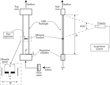
A series of experiments were carried out in a shallow-water channel of thickness $d=1~\text{cm}$ , width $W=15~\text{cm}$ and length $H=100~\text{cm}$ , with a lid on the base and top of the tank. A submerged pump fed the channel with fresh water from a reservoir whose volume was much larger than the channel. The flow rate was measured using a flow meter located upstream of the inlet section of the channel. In order to reduce any non-uniformity in the inflow, a flow straightener was located within a stagnation chamber from which the water was then forced into the channel (figure 1).

Figure 1.

Schematic representation of the experimental apparatus, with detail of the reference frame used for the experiments and of the notation used. It should be noted that the channel was horizontal during the experiments and there are both upper and lower lids to the tank.

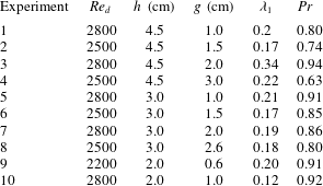
A series of different rectangular obstacles, each including a small gap through their centre, were inserted into the channel at a distance $40~\text{cm}$ downstream from the inlet section. Table 1 gives the dimensions ( $h$ ) and the gap ( $g$ ) of the different obstacles deployed. The outflow from the channel was connected to a drain, such that the channel was always fed with fresh water. The lower side of the channel was illuminated from the back using an LED uniform light source (Electroluminescent LightTape, Electro-LuminX Lighting Corp) producing a uniform illumination of the channel.

Table 1.

Experimental details: Reynolds number based on the channel depth ( $Re_{d}$ ), obstacle lateral dimension ( $h$ ), gap dimension ( $g$ ), momentum diffusivity constant ( $\unicode[STIX]{x1D706}_{1}$ ) and turbulent Prandtl number ( $\unicode[STIX]{x1D706}_{2}/\unicode[STIX]{x1D706}_{1}$ , where $\unicode[STIX]{x1D706}_{2}$ is the concentration diffusivity constant).

The experimental procedure consisted in first establishing a steady flux of fresh water through the channel. Red dye was then injected at a steady rate into the centre of the obstacle through an injection point located on the top wall of the channel using a peristaltic pump. The dye migrated downstream with the wake, mixing vertically and then being dispersed laterally through the eddies that developed in the wake downstream. A sequence of images of the top surface of the tank were captured using a Casio camera ( $f_{\#}=2.4$ , ISO 200) positioned above the channel such that the digital resolution was $9~\text{pixel}~\text{cm}^{-1}$ . The light intensity as recorded from the top surface of the channel could then be used to estimate the depth-averaged attenuation of the light caused by the presence of dye in the flow. In order to quantify the mixing of the flow, a calibration was performed to relate the light intensity to the depth-averaged concentration of dye, as described by Cenedese & Dalziel (Reference Cenedese, Dalziel, Carlomagno and Grant1998). In developing the calibration, the dyed fluid that was to be supplied at the obstacle in the steady flow was systematically diluted by undyed water, to provide 17 mixtures, $c_{i}$ , in which the dye concentration, $C_{i}$ , was a fraction $i/17$ of the original concentration of the dyed water, for $i=1,2,3,\ldots ,17$ . The channel was then filled with each of these mixtures in turn. The imaged area consisted of $131\times 550$ pixels. For each pixel, we developed an independent calibration curve by measuring the light intensity recorded at that pixel associated with each solution of known concentration. These curves were then used in the main experiment to estimate the depth-averaged concentration of the fluid at each point within the channel. Using this technique, we estimate that our measurements of the concentration are accurate to within a factor of $5\,\%$ .

For each experiment a sequence of at least 5000 frames was captured at a frequency equal to 120 Hz, so that ensemble average properties of the flow could be obtained. For each experiment, the Reynolds number ( $Re$ ) of the flow based on the thickness of the channel ( $d$ ) and the bulk flow speed ( $\overline{u}=Q/Wd$ ), $Re=\overline{u}d/\unicode[STIX]{x1D708}$ , is reported in table 1.

3 Experimental observations

3.1 Overall structure of the wake

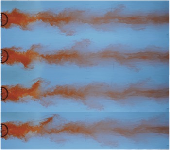
Figure 2 shows four images of the wake from experiment 2 (see table 1). The images show that the steady braid of dye, released from the centre of the obstacle, breaks up into a series of streaks spreading alternately on each side of the obstacle. This occurs as the dye released from the obstacle is engulfed and convected downstream by the eddies that are shed alternately from each side of the obstacle. This pattern of vortex shedding is in line with earlier reports that the flow has features resembling a vortex street (Chen & Jirka Reference Chen and Jirka1995). As the streaks of dye are stretched out by the eddies, they also become smeared out in the along-stream direction. We interpret this as being a result of the turbulent shear dispersion associated with the fluctuations in velocity across the depth of the channel (Taylor Reference Taylor1954). The figure suggests, however, that the cross-channel spreading of the dye into a series of streaks dominates the transport of the dye over a distance comparable to several multiples of the obstacle size, and in the following analysis of the data we test this picture of the control over the flow evolution and the dilution of the dye.

Figure 2.

Four photographs of the wake from experiment 2 in which the successive frames are taken at intervals of 0.25 s. The photographs illustrate how the continuous stream of red dye released at the obstacle becomes stretched out into a series of steaks around the eddies that are shed alternately from each side of the obstacle. Further downstream, these streaks of dye appear to become progressively mixed.

Figure 3.

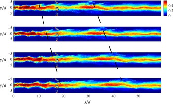
Variation of the concentration of the dye in the wake as a function of the position in the wake, shown at four equal time intervals of 0.25 s from experiment 2. The images are shown in false colour with the scale bar representing the concentration as a fraction of the concentration of the original dyed fluid released from the obstacle. The dashed lines track the downstream motion of specific eddies in this sequence of images.

Figure 4.

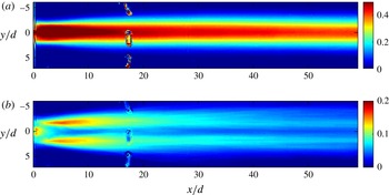
(a) Time-averaged dye concentration as a function of the position downstream of the obstacle, for experiment 2 (table 1), determined by averaging over 3600 frames corresponding to a 30 s interval during the experiment. The colour bar indicates the concentration of the dye relative to the source concentration. (b) Time average of the standard deviation of the concentration distribution as a function of position in the channel downstream of the obstacle, again for experiment 2.

Figure 5.

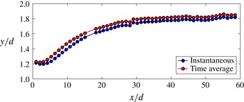
Second-order moment of the dye concentration showing the effective width of the wake as determined from the time average of the width measured in a series of instantaneous images (blue) and as determined from the time average of the concentration field (red) which includes the smoothing effect of the oscillation of the wake, as well as the actual mixing.

Figure 3 illustrates the evolution of the concentration of dye in a typical wake at four successive times, 0.25 s apart. In this figure, we have used false colour to illustrate the depth-averaged concentration of the dye as determined using our calibration curves. The darker red regions correspond to dye streaks convected by the eddies downstream of the obstacle. As these move downstream, they become progressively spread out, and a region of more dilute concentration, shown by the yellow and green colours, grows. The train of eddies shed from the obstacle appears to decay downstream as the velocity of the eddies relative to the mean flow wanes. As a result of the cross-channel mixing, the concentration of the dye also decays in the cross-channel direction, from a high value near the centre of the channel. However, there is a small cross-channel fluctuation in the location of this maximum concentration which arises from the alternating series of eddies shed from each side of the obstacle. We note that there is some noise in the image at a distance $x/d\sim 17$ in both figures 3 and 4. This corresponds to a series of dye injection nozzles which partially obscure the view of the tank at this location; since it is so localised, it does not impact our analysis of the evolution of the wake as described below, although it does lead to a small gap in the data shown in figure 5 at $x/d=17$ .

In the experiments, the dye concentration varies with the passage of the eddies and the associated fluctuation in the velocity field. It is of interest to understand the spatial distribution of the time-averaged concentration field, and the controls on this distribution. In figure 4(a), we present an example of the time-averaged concentration field, obtained from a time average of the data of experiment 2, and in figure 4(b) we show the variance of the concentration over time as measured relative to the mean concentration at each point. We have averaged 3600 images of the vertically averaged dye concentration, collected over a 30 s interval. This time average may be regarded as a convolution of the probability of there being an eddy or filament of dyed fluid at a particular point downstream with the degree of dilution of this fluid (Rocco & Woods Reference Rocco and Woods2015). It is seen that just downstream there is a rapid cross-channel spreading of the concentration, with a large variance. This is associated with the series of dye streaks that are convected downstream by the eddies alternating from one side of the obstacle to the other. However, the variance associated with this alternating series of eddies decays over a downstream distance of order 20–30 $d$ , and subsequently the concentration field is mainly located in the central region of the channel.

The time-averaged picture of the flow may include some apparent thickening of the wake as a result of the cross-channel oscillations. However, it is possible to show that this is a relatively small component of the total cross-channel width of the wake. For example, in figure 5 we compare (1) the width of the distribution of dye in the wake in the cross-channel direction using the time-averaged concentration profile (red line) with (2) the time average of the width of the instantaneous distribution of dye. The position of the centre of the distribution of dye, in the cross-channel direction, is given instantaneously by the relation

(3.1) $$\begin{eqnarray}y_{CG}(x,t)=\frac{\displaystyle \int _{-W/2}^{W/2}y(x)C(x,y,t)\,\text{d}y}{\displaystyle \int _{-W/2}^{W/2}C(x,y,t)\,\text{d}y}.\end{eqnarray}$$

The second-order moment of the instantaneous concentration distribution of dye relative to the instantaneous centre of the distribution provides an estimate of the instantaneous width of the wake,

(3.2) $$\begin{eqnarray}\unicode[STIX]{x1D70E}_{inst}(x)=\sqrt{\frac{\displaystyle \overline{\int _{-W/2}^{W/2}C(x,y,t)\cdot (y(x)-y_{CG}(x,t))^{2}\,\text{d}y}}{\displaystyle \int _{-W/2}^{W/2}C(x,y,t)\,\text{d}y}}.\end{eqnarray}$$

The time average of this instantaneous width is shown by the blue line as a function of position downstream of the obstacle. This is compared with the second-order moment of the time-averaged concentration field relative to the position of the centre of the time-averaged concentration field, shown by the red line,

(3.3) $$\begin{eqnarray}\unicode[STIX]{x1D70E}_{TA}(x)=\sqrt{{\displaystyle \frac{\displaystyle \int _{-W/2}^{W/2}\overline{C}(x,y)\cdot (y(x)-\overline{y}_{CG}(x))^{2}\,\text{d}y}{\displaystyle \int _{-W/2}^{W/2}\overline{C}(x,y)\,\text{d}y}}},\end{eqnarray}$$

where $W$ is the width of the channel and the overbar denotes the ensemble average operation. Figure 5 shows that the width of the time average profile (3.3) is approximately 1.05 times the width of the time average of the instantaneous profile (3.2). This difference arises from the fact that the time-averaged concentration includes the oscillation of the position of the wake, while the instantaneous measurement only accounts for the actual width relative to the centre of the wake at each time. Since the two moments (figure 5) only differ by a factor of 1.05 this implies that the fluctuations in width associated with the oscillations of the wake represent only a small fraction of the actual mixing across the wake.

Figure 6.

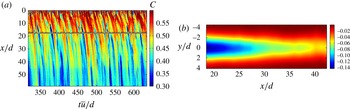
(a) Time series showing the false colour concentration along a line parallel to the axis of the channel, located at a distance $Y=2d$ from the centreline of the channel, using the data collected from experiment 2 (see table 1). The figure illustrates the intermittent passage of discrete streaks of dyed fluid along the channel, corresponding to the passage of eddies. The concentration gradually decreases as the flow migrates downstream, dilutes and gradually accelerates towards the background flow speed. The dilution may be recognised as the colour of the streaks gradually evolves down the channel from red to blue. (b) Ensemble average of the spatial distribution of the along-channel velocity, relative to the mean, $u/\overline{u}$ , as calculated from the speed of the streaks of dye measured from a series of images as shown in (a). In this figure, data are shown for experiment 2 (see table 1).

4 Model for the along-channel speed

Motivated by the above data illustrating the evolution of the time-averaged structure of the speed and concentration in the wake, we now aim to develop a model of the time-averaged properties of the wake incorporating the influence of both the bottom friction and the lateral mixing by the eddies. In developing a model of the evolving wake and the dilution associated with the eddies in the wake, it is convenient to work with the depth-averaged and time-averaged fields. In the model, we account for the time-dependent perturbations to the velocity field associated with (1) the alternating cycle of eddies that are shed from the each side of the obstacle and (2) the fluctuations in the velocity across the depth of the channel associated with the no-slip condition on the upper and lower surfaces of the channel. We assume that the no-slip condition leads to a frictional stress which can be parametrised in terms of a drag coefficient which depends on the Reynolds number of the flow (Moody Reference Moody1944). This approach is directly analogous to the parametrisation of the bottom friction as presented in earlier models of shallow-water flows (Seol & Jirka Reference Seol and Jirka2003; Negretti et al. Reference Negretti, Vignoli, Tubino and Brocchini2006). For the Reynolds numbers of the flow in the present experiments (table 1), the friction factor is of order $f\sim 0.04$ .

We write the depth-averaged velocity in the channel, $\boldsymbol{u}=(u,v)$ , in the form

(4.1) $$\begin{eqnarray}\boldsymbol{u}(x,y,t)=\overline{\boldsymbol{u}}(x)+\hat{\boldsymbol{u}}(x,y)+\tilde{\boldsymbol{u}}(x,y,t),\end{eqnarray}$$

where $\overline{\boldsymbol{u}}(x)$ is the cross-channel average of the time-averaged velocity, $\hat{\boldsymbol{u}}(x,y)$ is the variation of the time-averaged velocity from this cross-channel average and $\tilde{\boldsymbol{u}}(x,y,t)$ is the difference between the actual instantaneous velocity and the sum of these two time-averaged velocity fields. This leads to a depth-averaged equation of motion along the channel of the form

(4.2) $$\begin{eqnarray}\unicode[STIX]{x1D70C}\frac{\unicode[STIX]{x2202}\boldsymbol{u}}{\unicode[STIX]{x2202}t}+\unicode[STIX]{x1D70C}\boldsymbol{u}\boldsymbol{\cdot }\unicode[STIX]{x1D735}\boldsymbol{u}=\unicode[STIX]{x1D735}p-\frac{\displaystyle \unicode[STIX]{x1D70C}f}{\displaystyle 2d}|\boldsymbol{u}|\boldsymbol{u}.\end{eqnarray}$$

If we take the time average of (4.2), we find that the component in the along-channel direction has the form

(4.3) $$\begin{eqnarray}\unicode[STIX]{x1D70C}\overline{u}\frac{\unicode[STIX]{x2202}\hat{u} }{\unicode[STIX]{x2202}x}+\unicode[STIX]{x1D70C}\left<\tilde{u} \frac{\unicode[STIX]{x2202}\tilde{u} }{\unicode[STIX]{x2202}x}+\tilde{v}\frac{\unicode[STIX]{x2202}\tilde{u} }{\unicode[STIX]{x2202}y}\right>+\unicode[STIX]{x1D70C}\left(\hat{u} \frac{\unicode[STIX]{x2202}\hat{u} }{\unicode[STIX]{x2202}x}+\hat{v}\frac{\unicode[STIX]{x2202}\hat{u} }{\unicode[STIX]{x2202}y}\right)=-\frac{\unicode[STIX]{x1D70C}f}{2d}|\boldsymbol{u}|(\overline{u}+\tilde{u} )-\frac{\unicode[STIX]{x2202}p}{\unicode[STIX]{x2202}x},\end{eqnarray}$$

where $\langle \,\cdots \,\rangle$ denotes a time average. We expect the dominant balance in this equation to be between the along-channel pressure gradient, $(\unicode[STIX]{x2202}p/\unicode[STIX]{x2202}x)$ , and the frictional stress on the boundaries associated with the mean flow, $\unicode[STIX]{x1D70C}f|\boldsymbol{u}|\overline{u}/2d$ .

The remaining terms are associated with the disturbance to the flow resulting from the obstacle. Of these remaining terms, we might expect that the Reynolds stress, which is the second term on the left-hand side of (4.3), will balance the along-channel transport of the velocity shear (first term on the left-hand side), along with the frictional stress from the boundary associated with the perturbation to the velocity field. The Reynolds stress acts to diffuse the perturbation of the along-channel momentum in the cross-channel direction, leading to a gradual widening of the wake; the frictional stress acts to dissipate the perturbation in the along-channel momentum and is diffusive in character. In order to close the model, we therefore replace the Reynolds stress with an effective eddy viscosity $D$ . This acts on the perturbation to the along-channel velocity. As the perturbations to the mean velocity decay, we expect the balance

(4.4) $$\begin{eqnarray}\overline{u}\frac{\unicode[STIX]{x2202}\hat{u} }{\unicode[STIX]{x2202}x}=-f\frac{\overline{u}}{d}\hat{u} +\frac{\unicode[STIX]{x2202}}{\unicode[STIX]{x2202}y}\left(D\frac{\unicode[STIX]{x2202}\hat{u} }{\unicode[STIX]{x2202}y}\right),\end{eqnarray}$$

where we neglect terms of order $\hat{u} ^{2}$ in comparison to terms of order $\overline{u}\hat{u}$ , which is a good approximation for positions downstream in excess of $20d$ (see figure 6 b), and we assume that the downstream dispersive mixing by the Reynolds stress is small compared with the cross-channel dispersive mixing. This is consistent provided that the width of the wake, $Y$ say, is small compared with the distance downstream over which the wake decays, $X$ say, as we show below.

The mixing associated with the cross-channel fluctuations in the time-averaged velocity is produced by the stream of eddies moving downstream. We therefore expect that the dispersion coefficient $D$ will scale with the size of the eddies and the cross-channel fluctuation in the speed, leading to the relation

(4.5) $$\begin{eqnarray}D(x)=\unicode[STIX]{x1D706}_{1}\int _{0}^{W/2}\hat{\boldsymbol{u}}(x,y)\,\text{d}y,\end{eqnarray}$$

where $W/2$ is the half-width of the channel and $\unicode[STIX]{x1D706}_{1}$ is a constant. If we balance the along-channel advection (left-hand side of (4.4)) with the cross-channel dispersive mixing (second term on the right-hand side of (4.4)), we find that the width of the wake $Y\sim X\hat{u} /\overline{u}\ll X$ , consistent with our assumption that the cross-channel dispersion dominates the along-channel dispersion.

To proceed and develop solutions for (4.4), it is convenient to define an along-axis stretched coordinate $z$ using the relation

(4.6) $$\begin{eqnarray}z=\frac{1}{\overline{u}}\int _{0}^{x}D\,\text{d}x.\end{eqnarray}$$

Using this stretched coordinate, we find that equation (4.4) has a solution that can be expressed in the form

(4.7) $$\begin{eqnarray}\hat{u} (x,y)=\hat{A}\left(\frac{1}{z(x)}\right)^{1/2}\exp \left(-\frac{y^{2}}{4z}-\frac{fx}{d}\right).\end{eqnarray}$$

In this idealised solution, the point $x=0$ corresponds to the position of the virtual origin of the wake, at which there is a theoretical localised disturbance to the flow which leads to formation of the wake. In practice, immediately downstream of the actual obstacle, the flow adjusts towards this idealised solution and, once adjusted, it will then evolve according to the model above. In all of our experiments, in comparing the model with the data, we found that the best fit value for the location of the virtual origin relative to the centre of the obstacle is smaller than $d$ , the depth of the channel, and so in the remainder of the analysis we take the point $x=0$ to coincide with the centre of the obstacle.

We can use this solution for the cross-axis variation of $\hat{u}$ to calculate the dispersion coefficient

(4.8) $$\begin{eqnarray}D=\sqrt{\unicode[STIX]{x03C0}}A\unicode[STIX]{x1D706}_{1}\exp \left(-\frac{fx}{d}\right),\end{eqnarray}$$

and so

(4.9) $$\begin{eqnarray}z(x)=\frac{A\unicode[STIX]{x1D706}_{1}d\sqrt{\unicode[STIX]{x03C0}}}{fu}(1-\exp (-fx/d)).\end{eqnarray}$$

Combining the solution for $z$ with the expression for the velocity, we infer that

(4.10) $$\begin{eqnarray}\hat{u} (x,y)=\frac{Af\overline{u}}{\unicode[STIX]{x1D706}_{1}d\unicode[STIX]{x03C0}^{1/2}}\left(1-\exp \left(-\frac{y^{2}}{4z}\right)\right)\left(1-\exp \left(\frac{-fx}{d}\right)\right)^{1/2}.\end{eqnarray}$$

Equation (4.10) suggests that the cross-channel width of the wake scales as $Y\sim (4z)^{1/2}$ , and in moving downstream, equation (4.9) suggests that the width of the wake asymptotes to the value $(A\unicode[STIX]{x1D706}_{1}\sqrt{\unicode[STIX]{x03C0}}/fu)$ . The model also suggests that the velocity anomaly along the axis of the wake decays with distance as

(4.11) $$\begin{eqnarray}\hat{u} (x,0)=\frac{Af\overline{u}}{\unicode[STIX]{x1D706}_{1}\text{d}\unicode[STIX]{x03C0}^{1/2}}\exp \left(-\frac{fx}{d}\right)\left(\frac{1}{1-\exp (-fx/d)}\right)^{1/2}.\end{eqnarray}$$

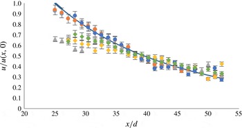
We have compared the variation of the speed in both the along-channel and cross-channel directions as predicted by the model with the experimental data from each of the experiments in table 1 in order to determine whether the functional form is consistent with the data, and also to estimate the best fit value of the parameter $\unicode[STIX]{x1D706}_{1}$ . In figure 7 we compare the experimentally measured value of the quantity $\hat{u} (x,0)$ , normalised to give the best fit to the model prediction, equation (4.11). The only free parameter in the model is the friction coefficient $f$ which we have set to value $0.04$ consistent with earlier experimental measurements (cf. Moody Reference Moody1944). The figure shows that in each experiment, for the region $30<x/d<60$ , there is good agreement between the model prediction of speed with distance along the channel and the experimental data, This suggests that the functional form for the decay along the channel as predicted by the model provides a good representation of the experimental observations. We have estimated the value $A\unicode[STIX]{x1D706}$ in the model relation (4.11) by finding the average value of the ratio of the measured velocity $\hat{u} (x,0)$ and the shape function $\exp (-(f/d)x)(1/1-\exp (-fx/d))^{1/2}$ as a function of the distance downstream. In order to determine $\unicode[STIX]{x1D706}$ , we now use the cross-channel variations in the speed of the flow.

Figure 7.

Variation in the time-averaged along-channel speed at the centreline of the channel, as a function of position along the channel, as measured in experiments 1–6 (table 1), and shown by the symbols (1, red circles; 2, green circles; 3, blue circles; 4, grey circles; 5, yellow circles; 6, green triangles). Each data set is rescaled to fit the model prediction ((4.11); blue line), which is calculated using the friction coefficient $f=0.04$ . Experiments 4, 5 and 6 require a greater distance for the speed to adjust to the model prediction; these experiments are characterised by having the widest opening within the obstacle relative to the width of the obstacle (table 1) and so cause the smallest perturbation to the flow.

Figure 8.

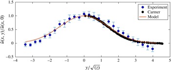
Comparison of the variation of the cross-channel velocity profile as measured in experiment 2 at a series of points downstream, with the mean value shown by the symbols and the standard deviation shown by the error bars, with the theoretical model prediction (solid line). Data presented by van Carmer et al. (Reference van Carmer, Rummel and Jirka2009) are also shown on this figure (black dots).

We have compared the variation of the speed in the cross-channel direction, as measured in the data, with the model prediction

(4.12) $$\begin{eqnarray}\hat{u} (x,y)=\frac{A}{\sqrt{(z)}}\exp \left(-\frac{y^{2}}{4z}\right).\end{eqnarray}$$

In order to compare the cross-channel variation of the speed at a series of positions along the channel, we have normalised the data with the local speed in the centre of the channel at that position. We can then compare the cross-channel velocity profile with the model prediction,

(4.13) $$\begin{eqnarray}\hat{u} (x,y)/\hat{u} (x,0)=\exp \left(-\frac{y^{2}}{4z}\right).\end{eqnarray}$$

Again, there is good agreement between the data and the model velocity profile as shown in figure 8 corresponding to the data from experiment 2. The error bars represent the variation in the velocity at each value of $y/\sqrt{(z)}$ as the position along the channel varies. We have also compared data presented by van Carmer et al. Reference van Carmer, Rummel and Jirka2009 for the variation of the along-channel velocity as a function of cross-channel position at one point down the channel as measured in their experiment. Again, this is in good agreement with the model profile (Negretti et al. Reference Negretti, Vignoli, Tubino and Brocchini2006).

For the suite of experiments listed in table 1, comparison of the model and the data suggests that the best fit value of the parameter $\unicode[STIX]{x1D706}_{1}$ is given by $\unicode[STIX]{x1D706}_{1}=0.2\pm 0.05$ . The size of the obstacle and of the gap in the centre of the obstacle varies from experiment to experiment. In each experiment, there is an adjustment zone as the flow adjusts to the model velocity profile, which in our experiments occurs in the region $15{-}20d$ immediately downstream of the obstacle. Beyond this region, the structure of the velocity field in the wake appears to follow the model described in (4.11) in the region $25<x/d<60$ .

5 Dispersive mixing

In figures 3 and 4, we illustrated how a passive tracer released into the wake becomes mixed in the cross-channel direction as it migrates downstream. We now explore whether this mixing can be described by a combination of the dispersion produced by the alternating eddies that are shed from the obstacle and the turbulent shear dispersion which results from the turbulent fluctuations across the depth of the channel. As with the velocity fluctuation downstream of the obstacle, we expect that in the near field, the mixing will be dominated by the alternating series of eddies shed from the obstacle, which carry streaks of dye downstream. However, as these decay due to the boundary friction, the dispersal of gradients in the dye concentration by the turbulent fluctuations in the flow across the depth of the channel will become increasingly dominant.

If we denote the time-averaged concentration field by $C(x,y)$ , then based on the above model of turbulent mixing, we expect that $C$ will vary along the channel according to the dominant advection–dispersion balance,

(5.1) $$\begin{eqnarray}\overline{u}\frac{\unicode[STIX]{x2202}C}{\unicode[STIX]{x2202}x}=D_{c}\frac{\unicode[STIX]{x2202}^{2}C}{\unicode[STIX]{x2202}y^{2}}.\end{eqnarray}$$

Here, the dispersion coefficient $D_{c}$ may depend on the eddy-driven mixing

(5.2) $$\begin{eqnarray}D_{ce}(x)=\unicode[STIX]{x1D706}_{2}\int _{0}^{W/2}\hat{u} (x,y)\,\text{d}y\end{eqnarray}$$

in a directly analogous fashion to the cross-channel mixing of the momentum (4.5), combined with the shear dispersion associated with the velocity fluctuations across the depth of the channel, $D_{ct}$ . This latter process is expected to scale as $D_{ct}=\unicode[STIX]{x1D706}_{3}\bar{u}d$ , where we estimate that the coefficient $\unicode[STIX]{x1D706}_{3}\sim 0.01$ (Taylor Reference Taylor1954). Equation (5.2) then suggests that the concentration evolves along the channel according to the relation

(5.3) $$\begin{eqnarray}C(x,y)=B\left(\frac{1}{\unicode[STIX]{x1D709}(x)}\right)^{1/2}\exp \left(-\frac{y^{2}}{4\unicode[STIX]{x1D709}}\right),\end{eqnarray}$$

where $\unicode[STIX]{x1D709}(x)=(D_{ce}d/f)(1-\exp (-fx/d))+D_{ct}x$ is a transformed coordinate for the along-channel position, equivalent to $z(x)$ but now also including the effect of the constant turbulent dispersion $D_{ct}$ . In practice, the dye is supplied from a small pipe in the centre of the obstacle, and then spreads out and mixes into the wake downstream. As with the velocity field, we expect this adjustment to occur in the region $z<15{-}20d$ . Comparing the magnitude of the eddy mixing and the shear dispersion, we expect that in the subsequent flow, the eddy mixing associated with the alternating series of eddies shed by the obstacle will dominate the Taylor-type dispersion in the region $x<60{-}70d$ , and in this region we expect $\unicode[STIX]{x1D709}\approx Pr\,z(x)$ , where $Pr=\unicode[STIX]{x1D706}_{2}/\unicode[STIX]{x1D706}_{1}$ . We now test this model using data from the present suite of experiments.

Figure 9.

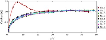
Variation of the time-averaged dye concentration at the centreline of the channel divided by $\sqrt{\unicode[STIX]{x1D709}}$ as a function of the position downstream. Data are shown for each of the experiments 1–8 as listed in table 1. In each case, the concentration has been normalised relative to the average value of the ratio $C/\sqrt{\unicode[STIX]{x1D709}(x)}$ in the region $25d<x<60d$ , so that all of the curves collapse.

Figure 10.

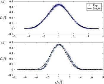
Experimental measurement of the time-averaged cross-channel dye concentration as a function of the cross-channel scaled coordinate $y/\sqrt{\unicode[STIX]{x1D709}}$ for experiment 2 (a) and 5 (b) (see table 1). The data are compared with the concentration profile predicted by the model. For each position along the channel, the data have been normalised by the concentration at the centreline of the channel, to enable comparison of the profiles at different points along the channel. Error bars are representative of the standard deviation of the time-averaged concentration at different points along the channel.

Figure 11.

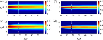
Comparison of the model prediction of the time-averaged concentration field downstream of the obstacle (a,b) and the experimental measurements (c,d) for experiments 2 (a,c) and 5 (b,d).

In figure 9, we show the time-averaged concentration as measured along the centreline of the channel, divided by $B\sqrt{(\unicode[STIX]{x1D709}(x))}$ . We have estimated $B$ as the average value of $C(x,0)/\sqrt{(\unicode[STIX]{x1D709}(x))}$ over the range $25d<x<60d$ . The figure shows that the ratio of the time-averaged concentration to the model prediction tends to a constant value in all experiments, suggesting that the functional form (5.3) describes the leading-order evolution of the concentration along the channel in the region $25d<x<60d$ . As may be seen from (5.3), this is primarily a function of the along-channel friction coefficient $f$ . In order to test the predicted scale for the cross-channel variation in concentration and determine a value for $\unicode[STIX]{x1D706}_{2}$ , in figure 10 we present experimental measurements of the concentration profile across the channel at various points along the channel for two representative experiments, 2 and 5. In each case, we show the variation of the scaled concentration $C\cdot \unicode[STIX]{x1D709}^{1/2}$ as a function of the scaled cross-channel position $y/\unicode[STIX]{x1D709}^{1/2}$ (5.3). The data at each point along the channel have been time-averaged. By choosing the best fit value of the model to these data, we estimate that $\unicode[STIX]{x1D706}_{2}=0.22$ for each experiment, with the difference between the data and the model prediction being less than $7\,\%$ for all of the experiments listed in table 1 (5.3).

To illustrate the time average of the spatial variation in concentration in more detail, in figure 11 we present the depth-averaged concentration fields as measured in experiments 2 and 5 (a,b), and as predicted by the model using the value of $\unicode[STIX]{x1D706}_{2}$ determined from the experiments above (c,d).