





1. Introduction
The resonant wave interaction approximation (RWIA) is used to simplify the study of nonlinearly interacting waves (e.g. Davis & Acrivos Reference Davis and Acrivos1967; Phillips Reference Phillips1981). The approximation restricts interactions to wave triads (or quartets when triad interactions are not possible) that satisfy a condition on the wave frequencies of the form
 $\omega _{\boldsymbol{k}}=|\omega _{\boldsymbol{p}}\pm \omega _{\boldsymbol{q}}|$
, in addition to the condition on the wavevectors
 $\boldsymbol{k}=\boldsymbol{p}+\boldsymbol{q}$
. The wave triads that satisfy both conditions form ‘resonance curves’ in the wavevector space, on which the significant interaction and energy transfer between waves with different wavevectors occur according to the theory. RWIA is used as part of the derivation of the kinetic equation of the weak wave turbulence formalism that aims to simplify the full nonlinear dynamics of weakly interacting wave fields (Hasselmann Reference Hasselmann1962; Zakharov Reference Zakharov1965; Nazarenko Reference Nazarenko2011; Zakharov et al. Reference Zakharov, L’vov and Falkovich2012).
The RWIA-based weak wave turbulence formalism has been applied to surface ocean waves (Hasselmann Reference Hasselmann1962), acoustic waves (L’vov et al. Reference L’vov, Lvov, Newell and Zakharov1997), internal waves in the ocean and atmosphere (e.g. Olbers Reference Olbers1976; McComas & Bretherton Reference McComas and Bretherton1977; Müller et al. Reference Müller, Holloway, Henyey and Pomphrey1986; Lvov et al. Reference Lvov, Polzin and Tabak2004), and the study of Rossby–gravity wave interactions (Eden et al. Reference Eden, Chouksey and Olbers2019a ). It has also been studied experimentally (e.g. Herbert et al. Reference Herbert, Mordant and Falcon2010; Rodda et al. Reference Rodda2022, Reference Rodda2023). The weak wave turbulence formalism is used to derive the closed kinetic equation for the energy spectrum. The resulting reduction in the number of interactions also leads to a more efficient computational treatment of the problem.
Our interest here is in the application of RWIA to the problem of a field of interacting internal waves in a stratified fluid. We critically examine the predictions of this approximation in the specific limited context of idealised two-dimensional (2-D) non-rotating simulations. For internal ocean waves, the observed wave spectrum has been shown to have some universal properties represented by the Garrett–Munk (GM) empirical fit (Garrett & Munk Reference Garrett and Munk1972, Reference Garrett and Munk1975; Cairns & Williams Reference Cairns and Williams1976; Garrett & Munk Reference Garrett and Munk1979; Levine Reference Levine2002), which was also studied in numerical simulations (e.g. Chen et al. Reference Chen, Chen, Liu, Xu, Xie, He and Cai2019; Pan et al. Reference Pan, Arbic, Nelson, Menemenlis, Peltier, Xu and Li2020) although deviations from the GM spectrum were observed (Wunsch & Webb Reference Wunsch and Webb1979; Polzin & Lvov Reference Polzin and Lvov2011; Pollmann Reference Pollmann2020; Le Boyer & Alford Reference Le Boyer and Alford2021). This spectrum is not fully understood despite decades of research. Nonlinear internal wave interactions and the resulting energy transfers and wave breaking are responsible for much of the mixing in the ocean interior (Munk & Wunsch Reference Munk and Wunsch1998). This mixing plays an important role in the absorption of CO
 $_2$
(Sabine et al. Reference Sabine2004), in forcing the large-scale meridional circulation and consequently in the global meridional ocean heat transport (Bryan Reference Bryan1987; Nikurashin & Ferrari Reference Nikurashin and Ferrari2013). The mixing occurs on scales smaller than can be represented in climate models. Its parametrisation requires an understanding of the nonlinear wave interactions, which the RWIA and the accompanying weak wave turbulence formalism aspire to provide.
The key assumption underlying the RWIA is that the wave amplitudes vary over a time scale longer than the corresponding linear wave periods. Different derivations of the RWIA approach this condition differently and, therefore, result in different slowness criteria. To study the self-consistency of the RWIA, one can initialise the RWIA-based kinetic equation for the internal wave field spectra with the GM spectrum and examine the time scale of the response. This (Boltzmann) time scale has been found to be inconsistent with the slowness assumption, posing a significant challenge to the theory (Holloway Reference Holloway1980; Lvov et al. Reference Lvov, Polzin and Yokoyama2012). Taking into account near-resonance interactions (L’vov et al. Reference L’vov, Lvov, Newell and Zakharov1997) was suggested to result in a slower and therefore self-consistent spectral adjustment time scale (Lvov et al. Reference Lvov, Polzin and Yokoyama2012). The ensemble-averaged rates of energy transfer due to wave–wave interactions in short, unforced, direct numerical simulations were found to be similar to those calculated using the kinetic equation (Eden et al. Reference Eden, Pollmann and Olbers2019b , Reference Eden, Pollmann and Olbers2020). The kinetic equation has also been shown to explain the transfer of energy between different regions of the spectrum (Dematteis et al. Reference Dematteis, Le Boyer, Pollmann, Polzin, Alford, Whalen and Lvov2024). The RWIA has also been applied to study 2-D internal waves, as we do here, and to derive the kinetic equation (Ripa Reference Ripa1981; Daubner & Zeitlin Reference Daubner and Zeitlin1996; Caillol & Zeitlin Reference Caillol and Zeitlin2000; Shavit et al. Reference Shavit, Bühler and Shatah2025; Labarre & Shavit Reference Labarre and Shavit2026). However, the question of the consistency of the kinetic equation and the assumptions used to derive it with the actual dynamics of typical oceanic internal wave fields, as opposed to the self-consistency of the kinetic equation, is still open.
In a recent work, Savva et al. (Reference Savva, Kafiabad and Vanneste2021) developed a linear kinetic equation to describe the scattering of internal waves by an assumed steady quasi-geostrophic (QG) flow. They find that the scattering leads to a cascade to small scales along surfaces of constant frequency in wavenumber space. The cascade results in an internal wave spectrum of the form
 $k^{-2}$
for scales smaller than the scale of the internal wave forcing, a cascade that develops without nonlinear wave–wave transfers. This spectrum is similar to the spectra observed in the atmosphere and ocean, suggesting an alternative to the shaping of the spectrum by wave–wave interaction, which is our focus here. Savva et al. (Reference Savva, Kafiabad and Vanneste2021) described the mechanism of interaction in the (WKBJ) limit, where internal wave wavelengths are smaller than QG scales, also analysed by Kafiabad et al. (Reference Kafiabad, Savva and Vanneste2019), as a version of the induced diffusion mechanism of McComas & Bretherton (Reference McComas and Bretherton1977), with the small-
 $K$
geostrophic mode playing the role of the low-frequency internal wave. They similarly identify the interaction of similar upward and downward propagating waves via scattering with the QG field as the elastic scattering mechanism of McComas & Bretherton (Reference McComas and Bretherton1977). Barkan et al. (Reference Barkan, Srinivasan and McWilliams2024) analysed the wave–eddy interaction using a coarse-graining approach in numerical simulations. They, again, show that the wave energy cascade is driven predominantly by scattering with eddies rather than via wave–wave interaction. Dong et al. (Reference Dong, Bühler and Smith2020) used the WKBJ approximation, allowing for slow time variation of the QG flow, and found that internal wave energy diffuses both along and across constant frequency surfaces, and Dong et al. (Reference Dong, Bühler and Smith2023) showed that even the interaction of waves with steady flow can lead to wave energy spreading off the constant frequency cone. However, Cox et al. (Reference Cox, Kafiabad and Vanneste2023) examine the role of a time-dependent QG flow and find the scattered wave spectrum to still be localised within a thin boundary layer around the constant-frequency cone. While the scattering of internal waves by a stationary or slowly varying QG flow may be a very efficient mechanism for cross-scale interactions, the fact that the resulting interactions are interpreted using terms that were derived based on the RWIA suggests that it is still worthwhile going back to this approximation and investigating its validity, as we do here. In addition, one does expect wave–wave interaction to dominate at small scales.
We follow three different derivations of the constraint on the frequencies of interacting waves represented by the RWIA that have been used as part of the weak wave turbulence formalism. Using direct numerical simulation (DNS) of idealised 2-D internal wave fields, forced at low wavenumbers and run to a statistical steady state (§ 2), we test the specific assumptions in each derivation that lead to the above-mentioned constraint on the frequencies. We also use the DNS, performed with the flow_solve model (Winters et al. Reference Winters, MacKinnon and Mills2004), to examine all nonlinear interactions in wavenumber space. We find that the dominant interactions are not necessarily on the resonance curves. That is, the nonlinear interaction term calculated from the DNS shows that many of the resonant interactions do not contribute significantly to energy transfers, while there are important interactions that are non-resonant. We note that the idealised settings used do not allow for making any claims regarding 3-D or observed internal waves, and that the derivation of the statistical theory for nonlinear wave–wave interaction for oceanic internal waves is developed in 3-D since its first report by Olbers (Reference Olbers1976) as well as in more recent derivations (e.g. Lvov & Tabak Reference Lvov and Tabak2004).
The derivation of the kinetic equation typically relies on ensemble averaging. It is possible, in principle, to test it using DNS with different random initial conditions or different realisations of the stochastic forcing. However, our testing of the assumptions leading to the resonance condition relies on analysing long, stochastically forced DNS that are at a statistical steady state. This implies that our testing involves time averaging rather than ensemble averaging.
2. Details of the numerical simulations
Numerical simulations of the 2-D Boussinesq equations (Appendix A) were performed with a double-periodic configuration of the flow_solve pseudospectral model (Winters et al. Reference Winters, MacKinnon and Mills2004). The size of the domain is
 $L_x=100$
km in the horizontal direction and
 $L_z=1$
km in the vertical direction. Most analyses use results with 512 grid points in the horizontal direction and 256 in the vertical direction, and we also show some results with double this resolution in both directions (
 $1024\times 512$
) to demonstrate robustness to resolution. A linear basic stratification is prescribed such that the Brunt–Väisälä buoyancy frequency is
 $N=(2\pi /30)$
min
 $^{-1}$
and the equations represent the full nonlinear dynamics of perturbations to this stratification (see Appendix A). We seek maximal simplification rather than relevance to ocean observations and, therefore, set the Coriolis force to zero. Each integration was carried out to a statistical steady state and then for 200 more days, which were used for the presented analyses. Our analyses are based on a high-frequency sampling of the model output at an interval of 18 s, allowing us to resolve all relevant motions and time derivatives from the output. The time step used for the integration is 1 s.
We use three runs with different amplitudes of temporally correlated stochastic forcing that is applied only to small wavenumbers of
 $0\lt |k_x|/(2\pi /L_x)\leqslant 2$
and
 $0\lt |k_z|/(2\pi /L_z)\leqslant 2$
, where
 $\boldsymbol{k}=(k_x,k_z)$
is the wavevector. The forcing is applied to the buoyancy equation (A2) and no forcing was applied directly to the momentum equations (A1). The stochastic forcing for each wavevector was set using a temporally correlated red-noise with a
 $\tau =1$
day correlation time,
 \begin{align} R&=\exp (-\Delta t/\tau ), \nonumber \\ \theta _n&=\theta _{n-1} R+\sigma \nu \sqrt {1-R^2}, \end{align}
where
 $\nu$
is a unit-amplitude random white noise and
 $\Delta t$
is the simulation time step. The stochastic forcing amplitudes of the different wavevectors are uncorrelated. The standard deviation of the medium forcing amplitude was three times larger than that of the weak one and the forcing of the strong run was five times that of the weakly forced run.
The eddy viscosity and diffusivity were set to the minimal values ensuring that a statistical steady state is achieved without numerical noise in the solution. The values used for the horizontal and vertical eddy viscosities are
 $\tilde {\nu }_x=0.2$
m
 $^2$
s−1 and
 $\tilde {\nu }_z=3\times 10^{-5}$
m
 $^2$
s−1. The diffusivity was assumed to be isotropic and was set to
 $\tilde {\kappa }_x=\tilde {\kappa }_z=3\times 10^{-5}$
m
 $^2$
s−1. We also simulated the dynamics using higher resolution of
 $1024\times 512$
and, for this simulation, the viscosity and diffusivity are reduced to
 $\tilde {\nu }_x=2.5\times 10^{-2}$
,
 $\tilde {\nu }_z=1\times 10^{-5}$
,
 $\tilde {\kappa }_x=\tilde {\kappa }_z=1.0\times 10^{-5}$
m
 $^2$
s−1.
Figure 1 shows the time series of the total energy density, and vertical and horizontal wavenumber energy spectra. The average energy levels of weakly, medium and strongly forced model runs are 0.41, 1.27 and 2.92 J m−3, respectively. The corresponding standard deviations (stds) of the energy time series are 0.02, 0.13 and 0.15 J m−3. Typical energy levels of ocean internal waves were estimated by Levine (Reference Levine2002) as 0.85
 $N/N_{\textit{ref}}$
J m−3, where
 $N_{\textit{ref}}=3$
cph. We use
 $N=2$
cph and this implies an expected energy of 0.6 J m−3, somewhere between the results of our simulations with weak and medium forcing amplitudes. Similarly, Lozovatsky et al. (Reference Lozovatsky, Morozov and Fernando2003) showed an energy density of 0.3–2 J m−3 depending on the distance from the mid-ocean bottom topography ridge where tidal energy is converted to internal waves. We therefore consider the energy levels of our weak and medium forcing cases to be in a range relevant to the dynamics of internal waves in the ocean. The simulated spectra in figure 1(b) show that the numerical eddy viscosity affects horizontal wavenumbers above 50 or so, where the spectra start decaying more rapidly beyond an inertial range not considerably affected by dissipation.
Characterising the energy in the direct 2-D numerical simulations. (a) Time series of standardised (mean removed, divided by std, with both specified in the figure legend) total energy per unit volume (J m−3) for 200 days for the three runs. (b) Energy spectra as a function of the horizontal wavenumber,
 $P(k_x)$
and (c) energy spectra as a function of the vertical wavenumber,
 $P(k_z)$
. The forced wavevectors are those with
 $0\lt |k_x|/(2\pi /L_x)\leqslant 2$
and
 $0\lt |k_z|/(2\pi /L_z)\leqslant 2$
.

Figure 1. Long description
Panel A: A line graph shows the standardized energy density over time for three different runs. The x-axis represents time in days, ranging from 0 to 200 days. The y-axis represents the standardized energy density, ranging from -4 to 4. Three lines are plotted: a blue line for weak energy, a black line for intermediate energy, and a red line for strong energy. The legend specifies the mean and standard deviation for each run. Panel B: A line graph displays the energy spectra as a function of the horizontal wavenumber. The x-axis represents the horizontal wavenumber normalized by 2π/Lx, ranging from 10^0 to 10^2. The y-axis represents the energy density, ranging from 10^-10 to 10^0. Three lines are plotted: a blue line for weak energy, a black line for intermediate energy, and a red line for strong energy. Panel C: A line graph shows the energy spectra as a function of the vertical wavenumber. The x-axis represents the vertical wavenumber normalized by 2π/Lz, ranging from 10^0 to 10^2. The y-axis represents the energy density, ranging from 10^-10 to 10^0. Three lines are plotted: a blue line for weak energy, a black line for intermediate energy, and a red line for strong energy.
3. Testing the results and assumptions behind derivations of the resonant-interaction approximation
We start with an outline of the derivation of the energy equation written in terms of wave amplitudes (§ 3.1). Next, we proceed to our main result (§ 3.2), which examines all interactions and shows that non-resonant interactions are important in our idealised 2-D simulations, although these simulations are weakly nonlinear and one would expect them to be consistent with the RWIA. We also show that resonant interactions in these simulations are not necessarily important, although that is not a surprise, as it is a well-known result that special triads dominate among resonant interactions (McComas & Bretherton Reference McComas and Bretherton1977). Finally, to understand why non-resonant interactions are important, we examine the assumptions behind three derivations of the approximation (§§ 3.3, 3.4, 3.5)
Different derivations of the RWIA rely on somewhat different assumptions, yet all are based on the wave amplitudes changing on a time scale longer than the linear wave period. Derivations of the RWIA have been presented using a continuous or discrete vertical representation of the internal wave field, using Eulerian, Lagrangian and isopycnal coordinates, as well as a Hamiltonian formulation, and more (Hasselmann Reference Hasselmann1966; Kenyon Reference Kenyon1968; Müller & Olbers Reference Müller and Olbers1975; McComas & Bretherton Reference McComas and Bretherton1977; McComas Reference McComas1977; Pomphrey et al. Reference Pomphrey, Meiss and Watson1980; Phillips Reference Phillips1981; Milder Reference Milder1982; Caillol & Zeitlin Reference Caillol and Zeitlin2000; Lvov & Tabak Reference Lvov and Tabak2001, Reference L’vov, Lvov, Newell and Zakharov2004), see a helpful summary of approaches to deriving the kinetic equation of weak wave turbulence in table 1 of Lvov et al. (Reference Lvov, Polzin and Yokoyama2012). Regardless of the basic approach, all derivations then use a variant of the slowness assumption to derive the constraint on the frequencies of interacting waves. We discuss three different derivations of this constraint that are motivated by derivations in the literature and test the validity conditions for each, using our model simulations.
3.1. Derivation of the energy equation in terms of wave amplitudes
We start by non-dimensionalising the momentum, buoyancy and continuity equations (Appendix A) and derive (Appendix B) non-dimensional equations for the vorticity (
 $\zeta =u_{z}-w_{x}$
) and buoyancy (
 $b=-g\rho /\rho _{0}$
) in physical space, with
 $(x,z)$
and
 $(u,w)$
being the coordinates and velocities in the horizontal and vertical directions, respectively, and with
 $\rho$
,
 $\rho _0$
and
 $g$
being the perturbation density relative to a specified linear mean stratification, a constant reference density and gravity acceleration. Let the Fourier transform of the vorticity be
 $\zeta _{\boldsymbol{k}}$
and the Fourier transform of the buoyancy be
 $b_{\boldsymbol{k}}$
, where
 $\boldsymbol{k}=(k_x,k_z)$
is the wavevector. We define a wave amplitude in the spectral space,
 $A_{a,\boldsymbol{k}}$
, (e.g. Carnevale Reference Carnevale1981) and calculate it from the output of our DNS,
 \begin{align} A_{a,\boldsymbol{k}}=\frac {1}{2}(\zeta _{\boldsymbol{k}}/k+ab_{\boldsymbol{k}}), \end{align}
where
 $k$
is the magnitude of the wavevector and
 $a=\pm 1$
, corresponding to right and left propagating waves. The dynamics of the wave amplitudes is described by
 \begin{equation} \frac {\partial {A}_{a,\boldsymbol{k}}}{\partial t} +\mathsf{L}_{ab}A_{b,\boldsymbol{k}} = \frac {\epsilon }{\left (4\pi \right )^{2}} {\int \limits _{-\infty }^{\infty }} \text{d}^{2}\boldsymbol{q}\,\text{d}^{2}\boldsymbol{p}\; \mathsf{M}_{\textit{abc}}(\boldsymbol{k},\boldsymbol{p},\boldsymbol{q}) \delta \left ( \boldsymbol{k}-\boldsymbol{p}-\boldsymbol{q}\right ) A_{b,\boldsymbol{p}}A_{c,\boldsymbol{q}}+F_{a}(\boldsymbol{k}), \end{equation}
where
 $t$
denotes the time and a sum over repeated indices (
 $b,c$
) is implied; note that when
 $b$
is used as a subscript, it is an index taking the values
 $\pm 1$
rather than referring to the buoyancy. Here,
 $\mathsf{L}=\mathsf{L}_w+\mathsf{L}_d$
is a linear operator representing the wave and dissipation parts,
 $\mathsf{M}_{\textit{abc}}(\boldsymbol{k},\boldsymbol{p},\boldsymbol{q})$
is a nonlinear interaction coefficient (Appendix B), and
 $\epsilon ={u_{0}}/{\textit{NL}_x}.$
is a dimensionless parameter characterising the ratio of the nonlinear and linear parts of the amplitude dynamics (Appendix A). The exact energy equation, in terms of the wave amplitudes in spectral space and with no approximations applied yet, is obtained by multiplying (3.2) by the complex conjugate of the wave amplitude,
 $A_{a,\boldsymbol{k}}^{\ast }$
(Appendix B),
 \begin{align} &\frac {\partial }{\partial t}\big( A_{a,\boldsymbol{k}}A_{a,\boldsymbol{k}}^{\ast }\big) =2\epsilon \textit{Re} \left (\frac {1}{4(2\pi)^{2}} {\int \limits _{-\infty }^{\infty }} \text{d}^{2}\boldsymbol{q}\,\text{d}^{2}\boldsymbol{p}\; \delta (\boldsymbol{k}-\boldsymbol{p}-\boldsymbol{q} ) \mathsf{M}_{\textit{abc}} (\boldsymbol{k},\boldsymbol{p},\boldsymbol{q}) A_{b,\boldsymbol{p}}A_{c,\boldsymbol{q}}A_{a,\boldsymbol{k}}^{\ast }\right ) \\ &\quad -2\textit{Re} \big (L_{ab}A_{b,\boldsymbol{k}}A_{a,\boldsymbol{k}}^{\ast } \big ) +2\textit{Re} \big (F_{a}^{\ast } ( \boldsymbol{k} ) A_{a,\boldsymbol{k}}\big ).\nonumber \end{align}
The part of this equation highlighted in blue is the ‘interaction term’ analysed in the following, representing the transfer of energy between wavevectors
 $\boldsymbol{p},\boldsymbol{q}$
and
 $\boldsymbol{k}$
. For linear dynamics, and in the absence of dissipation (
 $\mathsf{L}_{d}=0$
) and forcing (
 $F_a=0$
), the energy of any wave mode, right or left propagating (
 $a=\pm 1$
), is conserved.
(a–c) Time-average of the interaction term (
 $\mathsf{M}_{\textit{abc}}(\boldsymbol{k},\boldsymbol{p},\boldsymbol{k}-\boldsymbol{p}) A_{b,\boldsymbol{p}}A_{c,\boldsymbol{k}-\boldsymbol{p}}A_{a,\boldsymbol{k}}^{\ast }$
in (3.3)) for non-dimensional wavevectors
 $\boldsymbol{k}=(40,4)$
,
 $(24,12)$
and
 $(12,24)$
, for the medium forcing amplitude run, normalised (for each
 $\boldsymbol{k}$
) by its maximum value. The colour range corresponds to a part of the range of values plotted to include the weakest 10 % of the interactions, which account for approximately 50 % of the total energy transfers, as shown by figure 3. The positive values (red) correspond to gain and the negative ones (blue) to loss of energy by wavevector
 $\boldsymbol{k}$
. (d) A zoom into the region of
 $\boldsymbol{p}\sim \boldsymbol{k}$
for panel (c). The dashed and solid, blue, red and black lines represent the different resonance curves, see the text for details. The forced wavevectors are those with
 $0\lt |k_x|/(2\pi /L_x)\leqslant 2$
and
 $0\lt |k_z|/(2\pi /L_z)\leqslant 2$
.

3.2. Finding: some non-resonant interactions are important
The resonance condition implies that the nonlinear interaction term on the right-hand side of the energy equation,
 $\mathsf{M}_{\textit{abc}} (\boldsymbol{k},\boldsymbol{p},\boldsymbol{k}-\boldsymbol{p} ) A_{b,\boldsymbol{p}}A_{c,\boldsymbol{k}-\boldsymbol{p}}A_{a,\boldsymbol{k}}^{\ast }$
, is strong only if
 \begin{align} \Delta \omega (\boldsymbol{k},\boldsymbol{p},\boldsymbol{q},a,b,c) =a\omega _{\boldsymbol{k}}-b\omega _{\boldsymbol{p}}-c\omega _{\boldsymbol{q}}=0, \end{align}
where
 $a,b,c=\pm 1$
indicate the wave phase propagation direction, in addition to the condition on the wavevectors imposed by the delta function
 $\delta (\boldsymbol{k}-\boldsymbol{p}-\boldsymbol{q} )$
.
Figure 2 shows the time average of the nonlinear interaction term
 $\mathsf{M}_{\textit{abc}} (\boldsymbol{k},\boldsymbol{p},\boldsymbol{k}-\boldsymbol{p} ) A_{b,\boldsymbol{p}}A_{c,\boldsymbol{k}-\boldsymbol{p}}A_{a,\boldsymbol{k}}^{\ast }$
in (3.3) for the simulation with medium-amplitude forcing, for three different wavevectors
 $\boldsymbol{k}$
. The lines are solutions to
 $\boldsymbol{k}=\boldsymbol{p}+\boldsymbol{q}$
and the resonance condition
 $a\omega _{\boldsymbol{k}}-b\omega _{\boldsymbol{p}}-c\omega _{\boldsymbol{q}}=0$
, which may be reduced to
 $-\hat {\omega }_{\boldsymbol{k}}+\hat {\omega }_{\boldsymbol{p}}+\hat {\omega }_{\boldsymbol{q}}=0$
,
 $\hat {\omega }_{\boldsymbol{k}}+\hat {\omega }_{\boldsymbol{p}}-\hat {\omega }_{\boldsymbol{q}}=0$
or
 $\hat {\omega }_{\boldsymbol{k}}-\hat {\omega }_{\boldsymbol{p}}+\hat {\omega }_{\boldsymbol{q}}=0$
, where the hatted frequencies are positive,
 $\hat {\omega }_{\boldsymbol{k}}=|k_x|/\sqrt {k_x^2+k_z^2}$
. These are quadratic equations for, say
 $p_z$
as a function of
 $p_x$
(
 $\boldsymbol{k}$
is specified) and, therefore, there are six solutions for the resonant
 $p_z$
, corresponding to the six line types in the figure. The resonance corresponding to
 $\hat {\omega }_{\boldsymbol{q}}=\hat {\omega }_{\boldsymbol{k}}-\hat {\omega }_{\boldsymbol{p}}$
is shown by the blue curves, that satisfying
 $\hat {\omega }_{\boldsymbol{q}}=\hat {\omega }_{\boldsymbol{k}}+\hat {\omega }_{\boldsymbol{p}}$
in red and
 $\hat {\omega }_{\boldsymbol{q}}=\hat {\omega }_{\boldsymbol{p}}-\hat {\omega }_{\boldsymbol{k}}$
in black. Each resonance has two solutions, shown by the solid and dashed curves. With
 $\boldsymbol{k}$
specified, the interaction term becomes a function of
 $\boldsymbol{p}=(p_x,p_z)$
alone and its average is shown by the colour shading; as can be easily seen, it is of a large magnitude only for a small fraction of these resonant wavevectors. This interaction term, based on the triple product of wave amplitudes, is predicted by the weak wave turbulence theory to be dominated by its values on the resonant curves, as predicted, for example, by (2.1.11) of Zakharov et al. (Reference Zakharov, L’vov and Falkovich2012), at the limit of vanishing friction.
Cumulative sum over the interaction term for the weakly forced experiment that is shown in figure S1, which is the weak forcing equivalent of figure 2. The cumulative sum is calculated for positive interaction values as the cumulative sum over the sorted interaction values, and for negative values similarly as the cumulative sum over the sorted negative values. The cumulative sum is then normalised by the largest in absolute value of the positive and negative cumulative sums. The rate of change of the energy of the wavenumber shown in the title of each panel is the sum over all the interaction values shown in figure S1. Therefore, the cumulative sum shows that approximately 40 %–60 % of this rate of change is achieved by the sum over interaction values smaller than 10 % of the maximum interaction term values, bounded by the vertical dash lines.

We find that some non-resonant interactions are stronger than most resonant interactions. These are well demonstrated for the medium-amplitude forcing run in the zoomed-in figure 2(d), and in figures S1 and S2 of the supplementary material available at https://doi.org/10.1017/jfm.2026.11997 which show the average of the interaction term for the weakly and strongly-forced simulations. One can see darkly coloured pixels away from the resonance curves, involving unforced wavevectors
 $\boldsymbol{k}, \boldsymbol{p}$
and
 $\boldsymbol{q}$
. The colour bar range highlights weaker interactions: the interaction term is normalised by its maximum absolute value (the maximum is with respect to the different
 $p_x,p_z$
values), and the colour range corresponds to 10 % of this maximum value, allowing to see even the weaker interactions. Figure 3 shows the cumulative sum of the interaction term, showing that these 10 % weakest interactions correspond to approximately 50 % of the total energy transfers, justifying this colour range choice. Corresponding supplementary figures S3, S4 and S5 use colour scales spanning the full range of the interaction term.
The values of the non-dimensional nonlinearity parameter
 $\epsilon$
(Appendix A) for the three simulations are small:
 $6{\times }10^{-5}$
, 0.0001, 0.0002, for the weak, intermediate and strong forcing, respectively, suggesting that the RWIA should apply to all three runs, while the above-mentioned interaction term plots suggest that this is not the case. Figure 4 shows the average of the interaction term for a model run at twice the spatial resolution. As in the previous figures, many non-resonant pixels are highlighted, suggesting that the issues with RWIA in our idealised 2-D simulations are robust to the resolution. As a reminder, only wavevectors with non-dimensional wave numbers
 $0\lt |k_x|/(2\pi /L_x)\leqslant 2$
and
 $0\lt |k_z|/(2\pi /L_z)\leqslant 2$
are forced (§ 2). That is, only the wavevectors very close to the origin in figure 2 are directly forced. To test the sensitivity to the DNS resolution, we show in figure 4 the averaged interaction term for a case with double the resolution (
 $1024\times 512$
, see details in § 2). The results are robust: non-resonant interactions are still significant.
(a–c) Time-average of the interaction term (the expression in blue on the second line of (3.3)) for
 $\boldsymbol{k}=(40,4),\,(24,12)$
and
 $(12,24)$
, for the doubled resolution (
 $1024\times 512$
) run. The mean energy of this run is 0.7 J m−3, which is between the weak- and medium-forced runs shown in figure 1. The shown interaction values are normalised (for each
 $\boldsymbol{k}$
) by their maximum and the colour range shows the weakest 10 % to see a wider range of interacting wavenumbers, as discussed in figure 2. (d) A zoom into the region of
 $\boldsymbol{p}\sim \boldsymbol{k}$
for panel (c). The lines represent the resonance curves.

Figure 4. Long description
Panel A: A scatter plot shows normalized interaction values for wavenumber k = (40, 4). The x-axis is labeled px/(2π/Lx) and ranges from -20 to 40. The y-axis is labeled pz/(2π/Lz) and ranges from -20 to 40. The plot includes red and blue data points and several lines representing resonance curves. Panel B: A scatter plot shows normalized interaction values for wavenumber k = (24, 12). The x-axis and y-axis labels and ranges are the same as in Panel A. The plot includes red and blue data points and several lines representing resonance curves. Panel C: A scatter plot shows normalized interaction values for wavenumber k = (12, 24). The x-axis and y-axis labels and ranges are the same as in Panel A. The plot includes red and blue data points and several lines representing resonance curves. Panel D: A zoomed-in scatter plot shows normalized interaction values for wavenumber k = (12, 24) in the region of interest. The x-axis ranges from 0 to 15, and the y-axis ranges from 15 to 30. The plot includes red and blue data points and several lines representing resonance curves. The color bar on the right indicates the normalized interaction values, ranging from -0.10 to 0.10.
Interestingly, strong interactions (darker blue or red pixels) occur for triads in which two wavevectors are large and one is small (i.e. for
 $\boldsymbol{p}\approx \boldsymbol{k}$
or, equivalently,
 $\boldsymbol{q}\approx \boldsymbol{k}$
). The parametric subharmonic instability and induced diffusion interactions (McComas & Bretherton Reference McComas and Bretherton1977) also involve a small wavevector mode, although the strong interactions in the previous figures do not necessarily lie on the resonant lines where these special triads are defined. Furthermore, these special triad interactions are relevant only when the RWIA is valid, while we show indications in the following that the required conditions for the RWIA to hold are not met in our simulations. Another possible explanation of some of the dominant interactions in figure 2, between forced small wavevectors and larger ones, may be the generalised quasi-linear approximation (GQL; Marston et al. Reference Marston, Chini and Tobias2016). However, the same figure 2 (as well as the double resolution case in figure 4 and strongly forced run shown in figure S2) also shows strong interactions even between unforced wavevectors. It is, therefore, not clear that GQL approximation describes the dominant interactions for our three simulations.
We now consider three different derivations of the RWIA starting from the above-mentioned equations and test their assumptions against our simulations. Our goal is to understand why the RWIA does not explain the entire set of important interactions in our idealised 2-D simulations.
3.3. Examining a first derivation of the resonant interactions approximation
The first derivation considered here is based on a formal two-time scale perturbation approach applied to the amplitude equation (3.2). For details on this method, see Benney & Saffman (Reference Benney and Saffman1966) and § 11.2 of Bender & Orszag (Reference Bender and Orszag1978) or, in the context of the weak wave turbulence approach to internal waves, e.g. Caillol & Zeitlin (Reference Caillol and Zeitlin2000). We start by assuming that the solution can be expanded in the small parameter,
 $\epsilon$
, namely,
 \begin{align} A_{a,\boldsymbol{k}}=A_{a,\boldsymbol{k,}0} +\epsilon A_{a,\boldsymbol{k,}1}+\epsilon ^{2}A_{a,\boldsymbol{k,}2}+{\cdots}, \end{align}
and the slow time scale is defined as
 $\tau =\epsilon t$
. The zeroth-order variable simply satisfies the linear equation,
 \begin{align} \frac {\partial }{\partial t} A_{a,\boldsymbol{k,}0}+L_{ab}A_{b,\boldsymbol{k,}0} =F_{a}\left (\boldsymbol{k}\right ), \end{align}
with a solution for
 $\boldsymbol{k}$
away from the forced wavevectors of the form (neglecting dissipation and diffusion),
 \begin{align} A_{a,\boldsymbol{k,}0} =\hat {A}_{a,\boldsymbol{k}}\!\left ( \tau \right ) e^{-ia\omega _{\boldsymbol{k}}t}. \end{align}
The equation for the first order is
 \begin{align} &\frac {\partial }{\partial t} A_{a,\boldsymbol{k},1}+L_{ab}A_{b,\boldsymbol{k},1} =-\frac {\partial }{\partial \tau } A_{a,\boldsymbol{k},0} \nonumber \\ & +\frac {1}{4\!\left (2\pi \right )^{2}} {\displaystyle \int \limits _{-\infty }^{\infty }} \text{d}^{2}\boldsymbol{q}\text{d}^{2}\boldsymbol{p} \delta \left ( \boldsymbol{k}-\boldsymbol{p}-\boldsymbol{q}\right ) \mathsf{M}_{\textit{abc}}\left (\boldsymbol{k},\boldsymbol{p},\boldsymbol{q}\right ) A_{b,\boldsymbol{p},0}A_{c,\boldsymbol{q},0}. \end{align}
The right-hand side can be shown (Appendix C) to be proportional to
 $e^{-ia\omega (\boldsymbol{k})t}$
, which is the solution to the left-hand side operator and, thus, may result in a secular term that grows linearly in
 $t$
, a growth we want to bound so that the order
 $\epsilon$
terms remain smaller than the zeroth order and the perturbation series remains valid for long times. Requiring the coefficient of the secular term to vanish leads to the resonant interaction condition represented by (3.4), consistent with the RWIA whose testing is our focus here.
Consider a couple of caveats. For continuous fields of random waves, the bounded growth condition is applied to the energy density (see the discussion paragraph at the end of § 2.4 of Benney & Saffman (Reference Benney and Saffman1966)). For discrete spectra, such as those appearing in our finite domain simulations, the secular terms can be eliminated in the equation for the amplitudes for the perturbation expansion to be valid for large
 $t$
(see the above-mentioned discussion paragraph). There are, of course, other ways of defining a slowly varying wave amplitude, including a running-mean of
 ${A}_{a,\boldsymbol{k}}$
or the absolute value of
 $\hat {A}_{a,\boldsymbol{k}}$
. However, the derivations considered in this paper, including the one considered here, use the definition (3.7). Our objective is to test these derivations and, therefore, we use this definition.
This derivation depended on the wave amplitude
 $\hat A_{a,\boldsymbol{k}}$
varying with
 $\tau =\epsilon t$
and, thus, on a longer time scale than the linear wave period. To test whether such a slow amplitude approximation is consistent with our numerical simulations, we define a measure
 $V_1(\boldsymbol{k},a)$
, the ratio between the time scale of slow amplitude variations and the linear wave period. The time scale of the slow amplitude variations,
 $T(\hat {A}_{a,\boldsymbol{k}})$
, is estimated via the root mean square (r.m.s.) of its time derivative. The self-consistency of the first derivation of the RWIA requires that this measure satisfies
 \begin{align} V_1(\boldsymbol{k},a) =\frac {T(\hat {A}_{a,\boldsymbol{k}})}{{2\pi }/|\omega _{\boldsymbol{k}}|} =\left (\frac {1}{[\hat {A}_{a,\boldsymbol{k}}]} \left [\frac {\text{d}\hat {A}_{a,\boldsymbol{k}}}{\text{d}t}\right ]\right )^{-1} {|\omega _{\boldsymbol{k}}|}\gg 1. \end{align}
Here,
 $[\boldsymbol{\cdot }]$
indicates the r.m.s. of the real part of the quantity in the square brackets (the results for the imaginary part, which are not presented here, are similar). Figure 5 shows
 $V_1$
for all the resolved wavevectors and, clearly, for nearly all wavevectors except those with a small vertical wavenumber, it is not larger than one (the range smaller than one is shown by red shading), certainly not much larger. The contours in figure 5 show the spectral energy density
 $\log _{10}E(\boldsymbol{k})$
, making it clear that wavevectors with significant energy do not satisfy the slow-amplitude condition.
The reason for this is made clear in figure 6. The figure shows the fast and slow amplitudes for the weakly forced run for three different wavevectors. Even for the relatively short period waves in panel (c), the slow amplitude envelope shown by the blue line is not smooth and its time scale is therefore not larger than the time scale of the oscillating part. For the longer-period waves in the other two panels, it is difficult to distinguish between the wave amplitude and what was supposed to be the slow amplitude. A similar picture is seen for the more strongly forced experiments (figures S6, S7). In addition, supplementary table S1 shows the time scales calculated from the simulation for the same three wavenumbers analysed in figure S7 for the real, imaginary and absolute value of the slow wave amplitude. The results again indicate that these different time scale measures of the slow amplitude are not consistently much larger than the time scale of the linear wave.
Testing the slow amplitude assumption, requiring
 $V_1\gg 1$
, where
 $V_1$
is the ratio of the time scale of the slow amplitude and the linear wave period (3.9). Colour shading shows
 $V_1$
and the black contours show the spectral energy
 $\log _{10}E(\boldsymbol{k})$
with contour lines drawn from
 $-8$
to 2 with a contour interval of 1. (a) Weak, (b) intermediate and (c) strong forcing. The contour lines show that there is significant energy in wavenumbers that do not satisfy the slowness condition (red shading), spanning most resolved wavenumbers.

3.4. Examining a second derivation of the resonant interactions approximation
The standard derivation of the RWIA-based kinetic equation, in the context of weak wave turbulence, is based on the energy rather than the amplitude equation and typically uses ensemble averaging and a Gaussian decomposition of a fourth-order amplitude product. The second derivation of the RWIA we consider is based on the energy equation, while still avoiding ensemble averaging and the Gaussian assumption. We proceed by separating the wave amplitudes into a slow part and an oscillating term,
 ${A}_{a,\boldsymbol{k}}(t)=\hat {A}_{a,\boldsymbol{k}}(t)e^{-ia\omega _{\boldsymbol{k}}t}$
, temporally averaging the energy (3.3) over a time
 $T$
, and neglecting dissipation and forcing terms, to find (Appendix D)
 \begin{align} & \frac {1}{T} \big ( \hat {A}_{a,\boldsymbol{k}}\hat {A}_{a,\boldsymbol{k}}^{\ast }\big)\big |_0^T = \textit{Re} \left (\frac {2\epsilon }{\left (4\pi \right )^{2}} {\int \limits _{-\infty }^{\infty }} \text{d}^{2}\boldsymbol{q}\,\text{d}^{2}\boldsymbol{p} \right. \notag \\ &\, \left. \times \delta \left (\boldsymbol{k}-\boldsymbol{p}-\boldsymbol{q}\right ) {\sum \limits _{b,c}} \mathsf{M}_{\textit{abc}}\left ( \boldsymbol{k},\boldsymbol{p},\boldsymbol{q}\right ) \times \frac 1T\int \limits _0^T \hat {A}_{b,\boldsymbol{p}}\hat {A}_{c,\boldsymbol{q}}\hat {A}_{a,\boldsymbol{k}}^{\ast } e^{-i\left (-a\omega _{\boldsymbol{k}}+b\omega _{\boldsymbol{p}}+c\omega _{\boldsymbol{q}}\right )t}\,\text{d}t \right )\!. \end{align}
Now, assume that the product of the three slow amplitudes varies slower than the oscillating exponent in the last line of this equation. The slowness of the amplitudes is used to simplify the integral in the last line, which we denote as
 \begin{align} Y_{a,b,c}(\boldsymbol{k},\boldsymbol{p},\boldsymbol{q})=\textit{Re} \left (\frac 1T \int _0^T\hat {A}_{b,\boldsymbol{p}}\hat {A}_{c,\boldsymbol{q}} \hat {A}_{a,\boldsymbol{k}}^{\ast } e^{-i\left (-a\omega _{\boldsymbol{k}} +b\omega _{\boldsymbol{p}} +c\omega _{\boldsymbol{q}}\right )t}\,\text{d}t\right )\!. \end{align}
Under this slowness assumption, we can separate the slow triple product and the oscillating term and write the averaged expression as the product of averages. In the limit
 $T\to \infty$
, the average over the exponential term leads to the term
 $\delta _{0,\Delta \omega }$
, which is 1 if
 $\Delta \omega =0$
and zero otherwise, thus enforcing the resonance condition given by (3.4). Denoting the time average over a time
 $T$
as
 $\overline {(\boldsymbol{\cdot })}$
, this approximation can be written as
 \begin{align} X_{a,b,c}(\boldsymbol{k},\boldsymbol{p},\boldsymbol{q})&\equiv \textit{Re} \left (\overline {\hat {A}_{b,\boldsymbol{p}} \hat {A}_{c,\boldsymbol{q}} \hat {A}_{a,\boldsymbol{k}}^{\ast }} \;\times \; \frac {1}{T}\int \limits _0^T e^{i\Delta \omega (\boldsymbol{k},\boldsymbol{p},\boldsymbol{q},a,b,c) t}\,\text{d}t\right ) \\ &\quad\underset {T\to \infty }{\to } \textit{Re} \left (\overline {\hat {A}_{b,\boldsymbol{p}} \hat {A}_{c,\boldsymbol{q}} \hat {A}_{a,\boldsymbol{k}}^{\ast }} \right ) \delta _{0,\Delta \omega },\nonumber \end{align}
where
 $\Delta \omega (\boldsymbol{k},\boldsymbol{p},\boldsymbol{q},a,b,c)$
is defined in (3.4). The two quantities,
 $X$
and
 $Y$
, should be approximately the same for the RWIA derivation to be valid. We now define a quantitative measure of the difference between these two quantities. Crudely, this measure can be thought of as being the difference between
 $X$
and
 $Y$
divided by the maximum of the two, and calculated for each wavevector
 $\boldsymbol{p}=(p_x,p_z)$
.
Time series of the fast and slow amplitudes of three particular wavevectors in the weakly forced simulation. These panels demonstrate that the slow amplitude (blue) varies on a time scale not much longer than that of the linear wave period, as also quantified in figure 5.

Figure 6. Long description
Three line graphs show the time series of fast and slow amplitudes for different wavevectors in a weakly forced simulation. Panel A: The line graph displays the time series of fast and slow amplitudes for the wavevector k = (12, 24). The x-axis represents time in days, ranging from 0 to 20 days. The y-axis represents the amplitude Ak, ranging from -1.0 to 1.0. The red line represents the fast amplitude Ak, and the blue line represents the slow amplitude Ak (slow). The period of the fast wave is 4.2 days, and the period of the slow amplitude is 1.9 days. Panel B: The line graph displays the time series of fast and slow amplitudes for the wavevector k = (24, 12). The x-axis represents time in days, ranging from 0 to 20 days. The y-axis represents the amplitude Ak, ranging from -1.0 to 1.0. The red line represents the fast amplitude Ak, and the blue line represents the slow amplitude Ak (slow). The period of the fast wave is 1 day, and the period of the slow amplitude is 1.8 days. Panel C: The line graph displays the time series of fast and slow amplitudes for the wavevector k = (40, 4). The x-axis represents time in days, ranging from 0 to 20 days. The y-axis represents the amplitude Ak, ranging from -0.5 to 0.5. The red line represents the fast amplitude Ak, and the blue line represents the slow amplitude Ak (slow). The period of the fast wave is 0.21 days, and the period of the slow amplitude is 1.8 days.
Fixing
 $\boldsymbol{k}$
and given the delta function over the three wavevectors which imposes
 $\boldsymbol{q}=\boldsymbol{k}-\boldsymbol{p}$
, the difference between
 $X$
and
 $Y$
becomes a function of only the components of
 $\boldsymbol{p}=(p_x,p_z)$
and the three indices
 $a,b,c$
. To quantify the difference between the two, we use the following measure, which, for each value of
 $(p_x,p_z)$
, looks at the maximum over all values of
 $a,b,c$
of the absolute value of the difference between
 $X$
and
 $Y$
:
 \begin{align} V_{2}(\boldsymbol{k},\boldsymbol{p},\boldsymbol{q}) &=\textrm {sign}\left (X_{a*,b*,c*}(\boldsymbol{k},\boldsymbol{p},\boldsymbol{q})-Y_{a*,b*,c*}(\boldsymbol{k},\boldsymbol{p},\boldsymbol{q}) \right ) \nonumber \\ &\times \max _{a,b,c}\frac {|X_{a,b,c}(\boldsymbol{k},\boldsymbol{p},\boldsymbol{q})-Y_{a,b,c}(\boldsymbol{k},\boldsymbol{p},\boldsymbol{q})|} {\mathrm{normalisation}(\boldsymbol{k},\boldsymbol{p})} \end{align}
The normalisation factor in the denominator is calculated as the maximum of
 $|X|$
and
 $|Y|$
over all
 $a,b,c$
values,
 \begin{align} \mathrm{normalisation}(\boldsymbol{k},\boldsymbol{p}) ={\displaystyle \max _{a,b,c}\left (|X_{a,b,c}(\boldsymbol{k},\boldsymbol{p},\boldsymbol{q})|,|Y_{a,b,c}(\boldsymbol{k},\boldsymbol{p},\boldsymbol{q})|\right )}. \end{align}
The starred indices
 $a*,b*,c*$
correspond to the values of
 $a,b,c$
that yield the maximal absolute value of the difference between
 $X$
and
 $Y$
at each value of the wavevector argument
 $\boldsymbol{p}=(p_x,p_z)$
. The normalisation limits
 $V_{2}(\boldsymbol{k},\boldsymbol{p},\boldsymbol{q})$
to the range
 $[-2,2]$
. If the assumption justifying the replacement of the average of the product by the product of averages is valid, the measure
 $V_2$
should be much smaller than one.
Figure 7 shows
 $V_2$
for the weakly forced simulation (for the other two simulations, see supplementary figures S8 and S9). In areas of the wavevector space where the interaction term is non-negligible (that is, for
 $\boldsymbol{p}\approx 0$
and for
 $\boldsymbol{q}=\boldsymbol{k}-\boldsymbol{p}\approx 0$
, figure S1), the values of
 $V_2$
are large and close to their maximal absolute value of 2, and are thus not consistent with this second derivation. While derivations in the literature simply assume
 $T\to \infty$
, it is far from obvious what integration time
 $T$
should be used in this test of the second derivation. Because our DNS are in a statistical steady state and we do not expect a significant trend in wave amplitudes, we chose a long integration time of 200 days. One might need to use a time that is a function of the wave periods appearing in the definition of
 $X$
and
 $Y$
. Yet, our results indicate that the assumption of a slow amplitude does not seem to hold for our idealised 2-D simulations in the context of this second derivation as well.
Testing whether the three-product of wave amplitudes varies slowly, as quantified by criterion
 $V_2$
, (3.13), for the weak forcing case, for the wavevectors denoted in the titles of each panel.

3.5. Examining a third derivation of the resonant interactions approximation
The commonly used derivation of the RWIA (Appendix E) considers the equation for the time derivative of the triple product appearing in the energy equation (3.3), where the right-hand side of this equation contains a four-product of the wave amplitudes. See, for example, Lvov et al. (Reference Lvov, Polzin and Yokoyama2012) for an application of the weak wave turbulence’s kinetic equation to internal waves based on a canonical Hamiltonian approach, or Nazarenko (Reference Nazarenko2011) where this derivation is applied to the generating function. One then applies an ensemble average, uses a Gaussian decomposition of the four-product, assumes a spatial translation invariance, and assumes that right- and left-propagating waves are uncorrelated. The equation describing the dynamics of the ensemble-averaged energy spectrum
 $E_{a,\boldsymbol{k}}(t)=\langle {}A_{a,\boldsymbol{k}}^*A_{a,\boldsymbol{k}}\rangle /V$
, where
 $\langle \boldsymbol{\cdot }\rangle$
denotes an ensemble average and
 $V$
is the volume, takes the following form, neglecting forcing and dissipation:
 \begin{align} \frac {\partial }{\partial t}E_{a}(\boldsymbol{k},t) &= \frac {1}{4(2\pi )^4}\textit{Re} \left ( \int \limits _{-\infty }^{\infty } \text{d}^{2}\boldsymbol{q}\,\text{d}^{2}\boldsymbol{p}\delta \left ( \boldsymbol{k}-\boldsymbol{p}-\boldsymbol{q}\right ) {\displaystyle \sum \limits _{b,c}} \mathsf{M}_{\textit{abc}}\left ( \boldsymbol{k},\boldsymbol{p},\boldsymbol{q}\right ) \right. \nonumber \\ & \left. \times \int \limits _0^t e^{i\left (a\omega _{\boldsymbol{k}}-b\omega _{\boldsymbol{p}}-c\omega _{\boldsymbol{q}}\right )(t-t')}\mathcal{G}(\boldsymbol{k},\boldsymbol{p},\boldsymbol{q},a,b,c,t') \,\text{d}t' \right )\!, \end{align}
where
 \begin{align} &\mathcal{G}(\boldsymbol{k},\boldsymbol{p},\boldsymbol{q},a,b,c,t')= \Big [\mathsf{M}_{\textit{abc}}\left (\boldsymbol{k},\boldsymbol{p},\boldsymbol{q}\right ) E_{b}(\boldsymbol{p},t') E_{c}(\boldsymbol{q},t')\nonumber \nonumber \\ &-\mathsf{M}_{\textit{bac}}\left (\boldsymbol{p},\boldsymbol{k},\boldsymbol{q}\right ) E_{a}(\boldsymbol{k},t')E_{c}(\boldsymbol{q},t') -\mathsf{M}_{cab}\left (\boldsymbol{q},\boldsymbol{k},\boldsymbol{p}\right ) E_{a}(\boldsymbol{k},t')E_{b}(\boldsymbol{p},t')\Big ]. \end{align}
For more details and the derivation of
 $\mathcal{G}$
, see Appendix E. The right-hand side of the energy equation then contains a time integral over products of the energy multiplied by
 $e^{i\Delta \omega t}$
(3.15). This integral is simplified (e.g. Caillol & Zeitlin Reference Caillol and Zeitlin2000; Lvov et al. Reference Lvov, Polzin and Yokoyama2012), assuming that the ensemble-averaged energy spectrum varies over a time scale that is longer than the wave periods. This is assumed to lead to an integral over
 $e^{i\Delta \omega t}$
and thus to a delta-function factor
 $\delta ({\Delta \omega })$
, representing the resonance condition, leading to the final kinetic equation.
However, to consider the time integral of (3.15) as the product of two integrals, a more proper assumption is that the time scale of the energy spectrum variation (and thereby of
 $\mathcal{G}$
) should be much larger than the linear time scale of the oscillating term,
 $2\pi /\Delta \omega$
. Letting
 $T_E$
be the time scale over which the ensemble-averaged energy varies, the condition for this third derivation to be valid is
 \begin{align} V_3(\boldsymbol{k},\boldsymbol{p},a,b,c)=\frac {2\pi }{\Delta \omega (\boldsymbol{k},\boldsymbol{p},\boldsymbol{k}-\boldsymbol{p},a,b,c)}\times \frac {1}{T_E} \ll 1. \end{align}
Given that, by definition,
 $\Delta \omega =0$
on resonance curves and that this linear time therefore diverges there, the time scale for energy variations,
 $T_E$
, cannot be longer than the linear time scale on the resonance curves and, therefore, the condition in (3.17) cannot be satisfied for strictly resonant interactions. Supplementary figure S10 shows
 $V_3$
, using a somewhat arbitrary
 $T_E=1$
day time scale, demonstrating that
 $V_3$
is also not small near the resonance curves, as expected. If significant interactions occur near resonance curves, rather than only on the curves, as has been suggested by L’vov et al. (Reference L’vov, Lvov, Newell and Zakharov1997) and Lvov et al. (Reference Lvov, Polzin and Yokoyama2012), this condition needs to be satisfied at least near the curves, even if it cannot be satisfied on the curves, for this derivation to be self-consistent.
4. Discussion and conclusions
Numerous previous studies applied the resonant wave interaction approximation (RWIA) and the weak wave turbulence kinetic equation to internal waves (e.g. Kenyon Reference Kenyon1968; McComas & Bretherton Reference McComas and Bretherton1977; Caillol & Zeitlin Reference Caillol and Zeitlin2000). The weak interaction hypothesis behind the kinetic equation was claimed to be inconsistent with observations (Holloway Reference Holloway1980), although the claim was disputed by more recent work (Dematteis et al. Reference Dematteis, Le Boyer, Pollmann, Polzin, Alford, Whalen and Lvov2024), while the self-consistency of the kinetic equation was carefully examined (e.g. Lvov et al. Reference Lvov, Polzin and Yokoyama2012). Yet, to the best of our knowledge, no prior effort has examined whether the nonlinear dynamics due to the interaction of internal waves is consistent with the assumptions underlying the derivation of the RWIA. Equally important, previous studies have not examined the entire range of resolved wavenumbers to test if all significant wave–wave interactions satisfy the resonance constraint. We note that Pan et al. (Reference Pan, Arbic, Nelson, Menemenlis, Peltier, Xu and Li2020) did examine a few specific cross-sections in wavenumber space to find that some resonant interactions were significant, but did not consider all such resolved interactions as we do here for a highly idealised non-rotating 2-D case.
Given the known differences between 3-D and 2-D systems, and the obvious importance of the Coriolis force in the ocean, it cannot be claimed that our results apply to the ocean’s internal waves. However, we are not the first to consider the weak wave turbulence formalism applied to 2-D internal waves, as was done, for example, by Ripa (Reference Ripa1981), Daubner & Zeitlin (Reference Daubner and Zeitlin1996) and Caillol & Zeitlin (Reference Caillol and Zeitlin2000), and more recently by Shavit et al. (Reference Shavit, Bühler and Shatah2025) and Labarre & Shavit (Reference Labarre and Shavit2026), who compared a 2-D simulated spectrum with the predictions of the kinetic equation. In this context, we set out to examine the consistency of the RWIA within the limited framework of idealised, 2-D, double periodic, non-rotating simulations. The weak forcing regime we study is consistent with that where the RWIA should hold. Yet, another important validity requirement for this approximation, of an infinite domain (Nazarenko Reference Nazarenko2011), cannot be satisfied in numerical simulations such as those used here.
We find that the dominant interactions in our direct numerical simulations are not necessarily resonant and that resonant interactions are mostly not significant in terms of their contributions to energy transfers between different wavevectors. To attempt to rationalise this, we examine three derivations of the RWIA. None of the three derivations considered is consistent with our direct numerical simulations because the assumption that the wave amplitudes or energy vary slower than the relevant linear wave time scales is violated even for our weakest forced simulation, and the time scale over which the slow amplitude changes at a given wavevector is therefore not much larger than the wave period, as is required by the derivations. The rapidly varying amplitudes in our simulations, despite the very weak forcing and nonlinear interactions, suggest that it may not be completely justified to think of the fluid motion as interacting linear internal waves, as such a description implies slowly varying wave amplitudes. We conclude that the RWIA does not seem to be consistent with the interactions seen in our idealised direct numerical simulations.
Our objective in this work was to test the RWIA in the particular application to 2-D non-rotating, double-periodic internal waves. Whether these results generalise is not obvious and beyond the scope of this work. Our simulations are meant to examine the RWIA in the simplest configuration. Many of our results, while carefully derived, rely on the adequacy and relevance of the direct numerical simulations employed here. The idealisations employed here, including the double periodic 2-D domain, are similar to those used in recent simulations of internal ocean waves (Sugiyama et al. Reference Sugiyama, Niwa and Hibiya2009; Eden et al. Reference Eden, Chouksey and Olbers2019a ; Chen et al. Reference Chen, Chen, Liu, Xu, Xie, He and Cai2019). Yet, the simulations span a range of no more than 2 orders of magnitude of wavevectors that are not dominated by the numerical model viscosity. We do not include the Coriolis force nor the abundant near-inertial motions generated in the ocean by the winds at the surface and by the interaction of internal tides with topography. Our use of 2-D versus 3-D simulations means that the number of resonant interactions in any range of wave frequencies is lower, potentially weakening the resonant interactions (Lvov et al. Reference Lvov, Nazarenko and Pokorni2006), and we further discuss this in the following paragraph.
The use of 2-D simulations also implies that we do not resolve vertical vorticity due to the horizontal shear of the horizontal velocity (vortical modes such as quasigeostrophic eddies), which was found to play an important role in scattering internal wave energy (Kafiabad et al. Reference Kafiabad, Savva and Vanneste2019; Savva et al. Reference Savva, Kafiabad and Vanneste2021; Young Reference Young2021; Cox et al. Reference Cox, Kafiabad and Vanneste2023; Barkan et al. Reference Barkan, Srinivasan and McWilliams2024). The system of equations we explore (A1) allows a steady-state solution of the form
 $u=u(z)$
,
 $w=0$
,
 $b=0$
. In a weakly nonlinear system, such a solution may play the role of a slowly varying vortical mode that exists in a 3-D system. This mode is also possible to interpret as the ‘condensates’ that were studied by Korotkevich et al. (Reference Korotkevich, Nazarenko, Pan and Shatah2024), who suggested a modification of the spectral diffusion equation that includes the effects of such condensates. Our simulations indeed do develop an
 $x$
-independent
 $u(z)$
mode. Equations (3.2) that we use include this mode and its interaction with other waves. Yet, to verify that this mode is not the reason for the non-resonant interactions we find to be dominant, we ran another simulation, where
 $\boldsymbol{u}(k_x=0)$
and
 $\boldsymbol{u}(k_z=0)$
are both set to zero. The results in figure S11 show that this does not affect the main result that non-resonant interactions are dominant. We also note that in the case of Korotkevich et al. (Reference Korotkevich, Nazarenko, Pan and Shatah2024), the condensates seem to contain a significant part of the energy, while this is not the case in our simulations (see the spectra in figure 1). Our use of a constant buoyancy frequency eliminates some nonlinear interactions that can occur only with non-uniform stratification (Sutherland Reference Sutherland2016). The nonlinearity parameter in our simulations (
 $\epsilon$
) seems to be exceedingly small, yet it would have been reassuring if we could identify an even smaller value where only resonant interactions dominate. Unfortunately, further reducing the nonlinearity by reducing the forcing amplitude means that the small numerical dissipation used for numerical reasons prevents the wave energy from spreading to large wavevectors, making the inertial range too small to be meaningful.
Another concern that may be raised regarding our analysis is that the simulations do not allow for a sufficient number of resonant interactions to be excited. The RWIA involves taking two limits: the system size going to infinity and the nonlinearity being very weak (e.g. Nazarenko Reference Nazarenko2011). In numerical simulations, the resolved wavenumbers are discrete and cannot be expected to lie exactly on the resonant curves. This might suggest that a discrete simulation cannot be used to test the RWIA. Of course, linear dissipation, which is included in our numerical model as diffusion and viscosity, will lead to broadening. In addition, it was shown that nonlinear interactions lead to the broadening of the resonance curves to include near-resonant interactions (L’vov et al. Reference L’vov, Lvov, Newell and Zakharov1997; Lvov et al. Reference Lvov, Polzin and Yokoyama2012; Pan & Yue Reference Pan and Yue2017; Zhang & Pan Reference Zhang and Pan2022) within the RWIA. This broadening implies that under the assumptions of the RWIA, near-resonance interactions are expected to dominate the energy transfer and allow an energy cascade to develop (Lvov et al. Reference Lvov, Nazarenko and Pokorni2006). It is difficult to estimate a priori the specific broadening for a given strength of the nonlinear interactions and numerical resolution. It is also not known theoretically what number of near-resonant interactions is required for weak wave turbulence to be well represented on a finite grid. To address these issues, we invoke the estimates of the nonlinear broadening of resonance curves estimated by Lvov et al. (Reference Lvov, Polzin and Yokoyama2012). They find that a Lorentzian broadening, with the width set to 0.5 times the sum of frequencies of the three interacting waves, leads to a self-consistent Boltzmann ratio. We analysed their suggested Lorentzian weight applied to near-resonance wavenumbers and considered any triad whose weight is larger than 0.75 to be an activated near-resonance interaction. For the three wavenumbers considered in our different figures, this broadening leads to 35 %–75 % of the wavevectors being activated(!). It seems, therefore, that our simulations contain a sufficient number of activated interactions within the near-resonance range of the RWIA for a realistic level of nonlinearity in observed ocean internal waves. Another mechanism that leads to the broadening of resonances and to the activation of near-resonant interactions was discussed by Janssen (Reference Janssen2003) and Annenkov & Shrira (Reference Annenkov and Shrira2006). We note that there are alternative estimates of the nonlinear broadening (Pan & Yue Reference Pan and Yue2017; Zhang & Pan Reference Zhang and Pan2022). They point out that the limit of infinite integration time that leads to the delta function corresponding to the resonant frequencies (see definition and limit of the function
 $\delta _T (\Delta \omega )$
in (D4) and (D5)) is not physical, as the wave amplitudes would be expected to vary over such a long time due to nonlinear interactions. As a result, they consider a finite time limit in which this function maintains a finite width and leads to the inclusion of near-resonance interactions to be more realistic. They conclude that this broadening justifies the application of the kinetic equation to the analysis of a finite-resolution DNS as we do here. A related broadened-resonance analysis and a resulting generalised kinetic equation were applied to the parametric subharmonic instability by Onuki & Hibiya (Reference Onuki and Hibiya2019). Any numerical simulations cannot strictly satisfy the large-box limit required for the kinetic equation to hold in the sense that this limit allows for enough strict resonances to exist (Nazarenko Reference Nazarenko2011). Yet, the previous discussion of processes leading to the broadening of resonances means that even at a finite system size, we expect to have enough activated resonances. While this discussion suggests that the discreteness and the finite domain size of the numerical simulation may not be major issues for our results, it would be good to use the same analysis approach with numerical simulations that use a much higher resolution and a larger domain size.
A final caveat is that our analysis of the assumptions used to derive the RWIA is based on time averaging, while the standard derivation (Appendix E) relies on ensemble averaging and the Gaussian decomposition of four-products of wave amplitudes. We have also not addressed a recent alternative derivation of the kinetic equation based on large deviations theory (Guioth et al. Reference Guioth, Bouchet and Eyink2022).
It is important to note that while we find issues with the assumptions used to derive the kinetic equation when tested in our highly idealised framework, the kinetic equation has been used successfully for explaining observed internal ocean characteristics. Onuki & Hibiya (Reference Onuki and Hibiya2018) and Olbers et al. (Reference Olbers, Pollmann and Eden2020), for example, showed that the kinetic equation can correctly estimate the decay rates of internal waves via the parametric subharmonic instability and the transfer of tidal energy to the wave continuum. Similarly, Lvov & Tabak (Reference Lvov and Tabak2001) showed that the kinetic equation, based on Hamiltonian formalism, results in a GM-like energy spectrum. Pan et al. (Reference Pan, Arbic, Nelson, Menemenlis, Peltier, Xu and Li2020) showed that in a high-resolution realistic simulation, scale-separated interactions, such as induced diffusion, are the most important mechanisms for the formation of the power-law spectrum. This last result is consistent with our finding of strong interactions with low wavenumbers in figure S1, although we note that non-resonant interactions with low wavenumbers are also important in our simulations. The kinetic equation was also used to study energy fluxes in stationary and non-stationary spectra (Dematteis & Lvov Reference Dematteis and Lvov2021, Reference Dematteis and Lvov2023).
We attempted to make the case that none of the idealisations used here, nor our model limitations, would necessarily mean that the RWIA should not have applied to our simulation results, given that the measure of the nonlinearity (
 $\epsilon$
here) is very small for all our simulations and that this weak nonlinearity is the basis for the slowness assumption used in all derivations of the RWIA. Our findings, while perhaps of limited applicability due to the limited numerical resolution and highly idealised setting, call for further testing of the assumptions underlying the RWIA in more sophisticated and realistic simulations following the methodology outlined here.
Supplementary material
Supplementary material is available at https://doi.org/10.1017/jfm.2026.11997.
Acknowledgements
We thank Kraig Winters for making the code of flow_solve available, and Yulin Pan, Nicolas Grisouard and Oliver Buhler for helpful comments and discussions. E.T. thanks the Weizmann Institute for its hospitality during parts of this work. G.B. thanks Ester Levi for a lifelong inspiration.
Funding
E.T. has been funded by the NSF Climate Dynamics Program grant AGS-1924538 and the Harvard Dean’s Competitive Fund for Promising Scholarship. G.B. acknowledges support by ISF under grant no. 547/23.
Declaration of interests
The authors report no conflict of interest.
Appendix A. Non-dimensionalisation
The dimensional momentum equations in terms of dimensional variables denoted with
 $\tilde {(\boldsymbol{\cdot })}$
are
 \begin{align} \widetilde {u}_{\widetilde {t}}+\boldsymbol{\widetilde {u}}\boldsymbol{\cdot }\widetilde {\boldsymbol{\nabla }}\widetilde {u} & =-\frac {1}{\rho _{0}}\widetilde {p}_{\widetilde {x}}+\widetilde {\nu }_{x}\frac {\partial ^{2}}{\partial \widetilde {x}^{2}}\widetilde {u}+\widetilde {\nu }_{z}\frac {\partial ^{2}}{\partial \widetilde {z}^{2}}\widetilde {u}, \nonumber \\[3pt] \widetilde {w}_{\widetilde {t}}+\boldsymbol{\widetilde {u}}\boldsymbol{\cdot }\widetilde {\boldsymbol{\nabla }}\widetilde {w} & =-\frac {1}{\rho _{0}}\widetilde {p}_{\widetilde {z}}+\widetilde {b}+\widetilde {\nu }_{x}\frac {\partial ^{2}}{\partial \widetilde {x}^{2}}\widetilde {w}+\widetilde {\nu }_{z}\frac {\partial ^{2}}{\partial \widetilde {z}^{2}}\widetilde {w}. \end{align}
Here,
 $\widetilde {\boldsymbol{x}}=[\widetilde {x},\widetilde {z}]$
is the [horizontal, vertical] dimensional position vector and the corresponding velocity vector is
 $\boldsymbol{\widetilde {u}}=[\widetilde {u},\widetilde {w}]$
. The equation for the buoyancy
 $\widetilde {b}=-g\widetilde {\rho }/\rho _{0}$
, where
 $\widetilde {\rho }$
is the dimensional density,
 $g=9.8$
m s
 $^{-2}$
is gravitational acceleration and
 $\rho _0=1000$
kg m−3, is
 \begin{align} \widetilde {b}_{\widetilde {t}}+\boldsymbol{\widetilde {u}}\boldsymbol{\cdot }\widetilde {\boldsymbol{\nabla }}\widetilde {b}+\widetilde {w}\overline {\widetilde {b}}_{\widetilde {z}}= \widetilde {\kappa }_{x}\frac {\partial ^{2}}{\partial \widetilde {x}^{2}}\widetilde {b}+\widetilde {\kappa }_{z}\frac {\partial ^{2}}{\partial \widetilde {z}^{2}}\widetilde {b}+\widetilde {f}^{(b)}\left ( \boldsymbol{\widetilde {x}},\widetilde {t}\right )\!. \end{align}
The incompressibility condition implies
 \begin{align} \widetilde {u}_{\widetilde {x}}+\widetilde {w}_{\widetilde {z}}=0. \end{align}
In our direct numerical simulations, we impose a constant mean stratification, which dictates the Brunt–Väisälä buoyancy frequency,
 $N$
, as
 $\overline {\widetilde {b}}_{\widetilde {z}}={N}^{2}$
.
To non-dimensionalise the equations, we choose the following length, time and velocity scales:
 \begin{equation} \widetilde {x}=xL_x,\quad \widetilde {z}=zL_z,\ \widetilde {t}=t/N,\quad \widetilde {u}=uu_{0},\quad \widetilde {w}=ww_{0}=w\,u_{0}\frac {L_z}{L_x}, \end{equation}
and the non-dimensionalisation of the pressure and buoyancy are given by
 \begin{align} \widetilde {p} & = pp_{0},\quad \text{where } \quad p_{0}=\rho _{0}L_x N u_{0},\nonumber \\ \widetilde {b} & =bb_{0},\quad \text{where } \quad b_{0}=\frac {L_z}{L_x}u_{0}N. \end{align}
Applying this to the momentum equations, one finds
 \begin{align} u_{t}+\epsilon {\boldsymbol{u}}\boldsymbol{\cdot }\boldsymbol{\nabla }u & =-p_{x}+\left ( \nu _{x}\frac {\partial ^{2}u}{\partial x^{2}} +\nu _{z}\frac {\partial ^{2} u}{\partial z^{2}}\right )\!, \notag \\ w_{t}+\epsilon {\boldsymbol{u}}\boldsymbol{\cdot }\boldsymbol{\nabla }w & =-p_{z}+b +\left (\nu _{x}\frac {\partial ^{2}w}{\partial x^{2}}+\nu _{z}\frac {\partial ^{2} w}{\partial z^{2}}\right )\!, \nonumber \\ b_{t}+\epsilon {\boldsymbol{u}}\boldsymbol{\cdot }\boldsymbol{\nabla }b+w & =\left ( \kappa _{x}\frac {\partial ^{2}b}{\partial x^{2}}+\kappa _{z} \frac {\partial ^{2} b}{\partial z^{2}}\right ) +f^{(b)}\left (\boldsymbol{x},t\right )\!, \nonumber \\ u_{x}+w_{z}&=0, \end{align}
where we defined the components of the dimensionless anisotropic eddy viscosity
 $\nu _{x}=\widetilde {\nu }_{x}/{\textit{NL}_x^{2}}$
and
 $\nu _{z}=\,\widetilde {\nu }_{z}/{\textit{NL}_z^{2}}$
, and the components of the dimensionless anisotropic eddy diffusivity,
 $\kappa _{x}=\widetilde {\kappa }_{x}/{\textit{NL}_x^{2}};\kappa _{z}=\widetilde {\kappa } _{z}/{\textit{NL}_z^{2}}$
. The dimensionless forcing term is
 \begin{align} f^{(b)}\left ( \boldsymbol{x},t\right ) =\frac {1}{Nb_{0}}\widetilde {f}^{(b)}\left ( \boldsymbol{\widetilde {x}},\widetilde {t}\right ). \end{align}
The non-dimensional parameter multiplying the nonlinear terms is
 \begin{align} \epsilon ={u_{0}}/{\textit{NL}_x}. \end{align}
The velocity scale appearing here is calculated as the r.m.s. of the horizontal velocity for each run, while
 $L_x$
and
 $L_z$
are the horizontal and vertical basins’ extents, respectively.
Appendix B. Derivation of the energy equation in spectral space
Based on the non-dimensional equations derived in the previous section (A6), we introduce a stream function
 $\psi$
such that
 $u=\psi _{z}$
and
 $w=-\psi _{x}$
so that the vorticity is
 $\zeta =u_{z}-w_{x}=\boldsymbol{\nabla} ^{2}\psi$
. One can take the curl of the momentum equations to derive a vorticity equation and rewrite the buoyancy equation to find
 \begin{align} \zeta _{t}-(\nu _x\zeta _{xx}+\nu _z\zeta _{zz})+b_{x} & =\epsilon J(\psi ,\zeta ), \nonumber \\ b_{t}-(\kappa _xb_{xx}+\kappa _zb_{zz})-\psi _{x} & =\epsilon J(\psi ,b)+f^{b}(\boldsymbol{x},t). \end{align}
Here,
 $J(a,b)\equiv {}a_xb_z-a_zb_x$
. Fourier transforming (B1) yields
 \begin{align} &\dot {\zeta }_{\boldsymbol{k}} +(\nu _{x}k_{x}^{2}+\nu _{z}k_{z}^{2})\zeta _{\boldsymbol{k}} +ik_{x}b_{\boldsymbol{k}} =\epsilon (2\pi )^{-2}\int _{-\infty }^{\infty }\!\!\!\text{d}^{2}\boldsymbol{p}\,\text{d}^{2}\boldsymbol{q}\, \delta (\boldsymbol{p}+\boldsymbol{q}-\boldsymbol{k})(p_{x}q_{z}-p_{z}q_{x})p^{-2} \zeta _{\boldsymbol{p}}\zeta _{\boldsymbol{q}} \nonumber \\ &\dot {b}_{\boldsymbol{k}}+(\kappa _x k_x^{2}+\kappa _zk_z^2)b_{\boldsymbol{k}}+ik_{x}\zeta _{\boldsymbol{k}}k^{-2} \nonumber \\ &=\epsilon (2\pi )^{-2}\int _{-\infty }^{\infty }\!\!\!\text{d}^{2}\boldsymbol{p}\,\text{d}^{2}\boldsymbol{q}\, \delta (\boldsymbol{p}+\boldsymbol{q}-\boldsymbol{k})(p_{x}q_{z}-p_{z}q_{x})p^{-2} \zeta _{\boldsymbol{p}}b_{\boldsymbol{q}} + f^{b}(\boldsymbol{k},t). \end{align}
Here,
 $f^{b}(\boldsymbol{k},t)$
is the Fourier transform of the forcing term of the buoyancy equation. Next, we define a new variable (e.g. Carnevale Reference Carnevale1981),
 $A_{a,\boldsymbol{k}}$
, which is a wave amplitude,
 \begin{align} A_{a,\boldsymbol{k}}=\frac {1}{2}(\zeta _{\boldsymbol{k}}/k+ab_{\boldsymbol{k}}), \end{align}
where
 $a=\pm 1$
represents right- and left-propagating waves. The equation of motion for the wave amplitude in the spectral domain takes the form,
 \begin{align} \dot {A}_{a,\boldsymbol{k}}+\mathsf{L}_{ab}(\boldsymbol{k})A_{b,\boldsymbol{k}} =\epsilon {\sum _{\boldsymbol{p},\boldsymbol{q}}}{\sum \limits _{b,c}} \delta \left (\boldsymbol{k}-\boldsymbol{p}-\boldsymbol{q}\right ) \mathsf{M}_{\textit{abc}}(\boldsymbol{k},\boldsymbol{p},\boldsymbol{q})A_{b,\boldsymbol{p}}A_{c,\boldsymbol{q}}+F_{a}(\boldsymbol{k}), \end{align}
where the interaction coefficient
 $\mathsf{M}_{\pm }$
and the linear operator
 $\mathsf{L}$
, which represent both the wave and the dissipation, are
 \begin{align} \mathsf{M}_{\pm {}}(\boldsymbol{k},\boldsymbol{p},\boldsymbol{q}) &=\frac {p_{x}q_{z}-p_{z}q_{x}}{kpq} \left (\begin{array}{cc} q^{2}-p^{2}\pm k(q-p) & q^{2}-p^{2}\mp k(q+p)\\[7pt] q^{2}-p^{2}\pm k(q+p) & q^{2}-p^{2}\mp k(q-p) \end{array}\right )\!, \nonumber \\[3pt] \mathsf{L}_\mathsf{d}(\boldsymbol{k})&=\left ( \begin{array}[c]{cc} \frac {1}{2}\left ( \nu _{x}+\kappa _{x}\right ) k_{x}^{2}+\frac {1}{2}\left ( \nu _{z}+\kappa _{z}\right ) k_{z}^{2} & \frac {1}{2}\left ( \nu _{x}-\kappa _{x}\right ) k_{x}^{2}+\frac {1}{2}\left ( \nu _{z}-\kappa _{z}\right ) k_{z}^{2}\\[11pt] \frac {1}{2}\left ( \nu _{x}-\kappa _{x}\right ) k_{x}^{2}+\frac {1}{2}\left ( \nu _{z}-\kappa _{z}\right ) k_{z}^{2} & \frac {1}{2}\left ( \nu _{x}+\kappa _{x}\right ) k_{x}^{2}+\frac {1}{2}\left ( \nu _{z}+\kappa _{z}\right ) k_{z}^{2} \end{array} \right )\!, \nonumber \\[3pt] \mathsf{L}_\mathsf{w}(\boldsymbol{k})&=\left ( \begin{array}[c]{cc} +i{k_{x}}/{k} & 0 \\[9pt] 0 & -i{k_{x}}/{k} \end{array}\right )\!,\quad \mathsf{L}=\mathsf{L}_\mathsf{w}+\mathsf{L}_\mathsf{d}. \end{align}
The linear wave solution, ignoring all forcing, friction and nonlinear terms is
 ${A}_{a,\boldsymbol{k}}={A}_{a,\boldsymbol{k}}(0)e^{-ia(k_x/k)t}$
, and the corresponding non-dimensional frequency is given by
 $a(k_x/k)$
. The forcing term
 $F_{s}(\boldsymbol{k},t)=sf^{b}(\boldsymbol{k},t)/2$
in the amplitude (B4) is due to the forcing terms appearing in (B2). The energy equation in terms of the wave amplitudes is
 \begin{align} &\frac {\partial }{\partial t} \left (A_{a,\boldsymbol{k}}A_{a,\boldsymbol{k}}^{\ast }\right ) =-2\textit{Re} \left ({\sum \limits _{b}} L_{ab}A_{b,\boldsymbol{k}}A_{a,\boldsymbol{k}}^{\ast }\right ) +2\textit{Re} \left (F_{a}^{\ast }\left ( \boldsymbol{k}\right ) A_{a,\boldsymbol{k}}\right ) \nonumber \\ &+\epsilon 2\textit{Re} \left (\frac {1}{4\left ( 2\pi \right )^{2}} {\int \limits _{-\infty }^{\infty }} \text{d}^{2}\boldsymbol{q\,}\text{d}^{2}\boldsymbol{p} \delta \left (\boldsymbol{k}-\boldsymbol{p}-\boldsymbol{q}\right ) {\sum \limits _{b,c}} \mathsf{M}_{\textit{abc}}\left (\boldsymbol{k},\boldsymbol{p},\boldsymbol{q}\right ) A_{b,\boldsymbol{p}}A_{c,\boldsymbol{q}}A_{a,\boldsymbol{k}}^{\ast }\right )\!. \end{align}
Appendix C. First derivation: a two-time scale perturbative approach
In the first derivation considered here of the resonant condition on the frequencies of interacting waves, one uses a multiple time scale perturbative approach. See Benney & Saffman (Reference Benney and Saffman1966), or as outlined in the context of internal waves by, e.g. Caillol & Zeitlin (Reference Caillol and Zeitlin2000), with the general multiple time scale perturbative method described in § 11.2 of Bender & Orszag (Reference Bender and Orszag1978). We start by assuming that the solution can be expanded in the small parameter,
 $\epsilon$
, namely,
 \begin{align} A_{s,\boldsymbol{k}}=A_{s,\boldsymbol{k,}0}+\epsilon A_{s,\boldsymbol{k,}1}+\epsilon ^{2}A_{s,\boldsymbol{k,}2}+{\cdots} = {\displaystyle \sum \limits _{m=0}^{\infty }} \epsilon ^{m}A_{s,\boldsymbol{k,}m}. \end{align}
We also assume a timescale separation, namely, we define a slow time
 $\tau =\epsilon t$
and the full time derivative is assumed to be of the form
 $( {\text{d}}/{\text{d}t})=({\partial }/{\partial t})+\epsilon ({\partial }/{\partial \tau })$
. By substituting the above-mentioned expansion in the amplitude equation ((3.2) in the main text), we find
 \begin{align} &\frac {\partial }{\partial t} {\displaystyle \sum \limits _{m=0}^{\infty }} \epsilon ^{m}A_{a,\boldsymbol{k},m}+\frac {\partial }{\partial \tau } {\displaystyle \sum \limits _{m=0}^{\infty }} \epsilon ^{m+1}A_{a,\boldsymbol{k},m}+L_{ar} {\displaystyle \sum \limits _{m=0}^{\infty }} \epsilon ^{m}A_{r,\boldsymbol{k},m}-F_{a}\left ( \boldsymbol{k}\right )\nonumber \\ &=\frac {\epsilon }{4\left (2\pi \right )^{2}} {\displaystyle \int \limits _{-\infty }^{\infty }} \text{d}^{2}\boldsymbol{q}\,\text{d}^{2}\boldsymbol{p} \delta \left (\boldsymbol{k}-\boldsymbol{p}-\boldsymbol{q}\right ) \mathsf{M}_{\textit{abc}}\left (\boldsymbol{k},\boldsymbol{p},\boldsymbol{q}\right ) {\displaystyle \sum \limits _{m=0}^{\infty }} \epsilon ^{m}A_{b,\boldsymbol{p},m} {\displaystyle \sum \limits _{m'=0}^{\infty }} \epsilon ^{m'}A_{c,\boldsymbol{q},m'}. \end{align}
The zeroth-order variable simply satisfies the linear equation,
 \begin{align} \frac {\partial }{\partial t} A_{a,\boldsymbol{k},0}+L_{ab}A_{b,\boldsymbol{k},0} =F_{a}\left (\boldsymbol{k}\right ), \end{align}
with a solution for
 $\boldsymbol{k}$
away from the forced wavevectors of the form (neglecting dissipation and diffusion),
 \begin{align} A_{a,\boldsymbol{k},0} =\hat {A}_{a,\boldsymbol{k}}\left ( \tau \right ) e^{-ia\omega _{\boldsymbol{k}}t}. \end{align}
The equation for the first order is
 \begin{align} &\frac {\partial }{\partial t} A_{a,\boldsymbol{k},1}+L_{ab}A_{b,\boldsymbol{k},1} =-\frac {\partial }{\partial \tau } A_{a,\boldsymbol{k},0} \nonumber \\ & +\frac {1}{4\left (2\pi \right )^{2}} {\displaystyle \int \limits _{-\infty }^{\infty }} \text{d}^{2}\boldsymbol{q}\,\text{d}^{2}\boldsymbol{p} \delta \left ( \boldsymbol{k}-\boldsymbol{p}-\boldsymbol{q}\right ) \mathsf{M}_{\textit{abc}}\left (\boldsymbol{k},\boldsymbol{p},\boldsymbol{q}\right ) A_{b,\boldsymbol{p},0}A_{c,\boldsymbol{q},0}. \end{align}
Substituting the solution of the zeroth order, the right-hand side becomes
 \begin{align} &e^{-ia\omega _{\boldsymbol{k}}t}\Bigg (\!-\frac {\partial }{\partial \tau }\hat {A}_{a,\boldsymbol{k}}\left ( \tau \right ) \nonumber \\ &+\frac {1}{4\left ( 2\pi \right )^{2}}{\int \limits _{-\infty }^{\infty }} \text{d}^{2}\boldsymbol{q}\,\text{d}^{2}\boldsymbol{p}\delta \left (\boldsymbol{k}-\boldsymbol{p}-\boldsymbol{q}\right ) \mathsf{M}_{\textit{abc}}\left (\boldsymbol{k},\boldsymbol{p},\boldsymbol{q}\right ) \hat {A}_{b,\boldsymbol{p}}\left (\tau \right ) \hat {A}_{c,\boldsymbol{q}}\left (\tau \right ) e^{i\Delta \omega (\boldsymbol{k},\boldsymbol{p},\boldsymbol{q},a,b,c)t}\Bigg ). \end{align}
This is proportional to
 $e^{-ia\omega (\boldsymbol{k})t}$
, which is the solution to the left-hand side operator and, thus, may result in a secular term that grows linearly in
 $t$
and invalidates the perturbation expansion for large
 $t$
by making the
 $O(\epsilon )$
term larger than the zeroth-order term. To prevent a secular term in the solution for the first-order variables, we demand that the expression in the parentheses, which is the coefficient of the term that leads to a secular term, vanishes. Because the first term in the parentheses is only a function of
 $\tau$
, this implies that the second term, the integral, should not be a function of
 $t$
as well. Indeed, assuming a large time
 $t$
, the rapidly oscillating exponent of
 $\Delta \omega$
will lead to the vanishing of the integral whenever
 $\Delta \omega \ne 0$
. This leads to the resonance condition,
 \begin{align} \Delta \omega (\boldsymbol{k},\boldsymbol{p},\boldsymbol{q},a,b,c) =a\omega _{\boldsymbol{k}}-b\omega _{\boldsymbol{p}}-c\omega _{\boldsymbol{q}}=0, \end{align}
also eliminating the
 $t$
dependence mentioned in the last sentence.
Appendix D. Second derivation: assuming a slowly varying triple correlation
Neglecting the viscosity and diffusion, the time-averaged energy (B6) in terms of the slow wave amplitudes becomes
 \begin{align} &\frac 1T\int _0^T\frac {\partial }{\partial t} \left (A_{a,\boldsymbol{k}}A_{a,\boldsymbol{k}}^{\ast }\right )\,\text{d}t =2\textit{Re} \Bigg (\frac {\epsilon}{4\left ( 2\pi \right ) ^{2}} {\displaystyle \int \limits _{-\infty }^{\infty }} \text{d}^{2}\boldsymbol{q}\,\text{d}^{2}\boldsymbol{p} \delta \left ( \boldsymbol{k}-\boldsymbol{p}-\boldsymbol{q}\right ) {\displaystyle \sum \limits _{b,c}} \mathsf{M}_{\textit{abc}}\left (\boldsymbol{k},\boldsymbol{p},\boldsymbol{q}\right ) \nonumber \\ & \times \frac {1}{T}\int _0^T \hat {A}_{a,\boldsymbol{k}}^{\ast }\hat {A}_{b,\boldsymbol{p}}\hat {A}_{c,\boldsymbol{q}} e^{i\Delta \omega (\boldsymbol{k},\boldsymbol{p},\boldsymbol{q},a,b,c)t}\,\text{d}t\Bigg ) +2\textit{Re} \left (\frac {1}{T}\int _0^TF_{a}^{\ast }\left ( \boldsymbol{k}\right ) e^{-ia\omega _{\boldsymbol{k}}t}\hat {A}_{a,\boldsymbol{k}}\,\text{d}t\right ). \end{align}
The right-hand side involves the following integral:
 \begin{align} Y_{a,b,c}(\boldsymbol{k},\boldsymbol{p},\boldsymbol{q})\equiv \textit{Re} \left (\frac {1}{T} \int \limits _0^T \hat {A}_{a,\boldsymbol{k}}^{\ast }\hat {A}_{b,\boldsymbol{p}}\hat {A}_{c,\boldsymbol{q}} e^{i\Delta \omega (\boldsymbol{k},\boldsymbol{p},\boldsymbol{q},a,b,c)t}\,\text{d}t\right). \end{align}
There are two possible paths to deriving the resonance condition leading to the kinetic equation starting from this equation. First, one assumes that the triple products of the slow amplitudes are uncorrelated with the deterministic phases; this reduces
 $Y_{a,b,c}(\boldsymbol{k},\boldsymbol{p},\boldsymbol{q})$
to
 \begin{align} X_{a,b,c}(\boldsymbol{k},\boldsymbol{p},\boldsymbol{q})&\equiv \textit{Re} \left(\frac {1}{T}\int \limits _0^T \hat {A}_{a,\boldsymbol{k}}^{\ast }\hat {A}_{b,\boldsymbol{p}} \hat {A}_{c,\boldsymbol{q}} \,\text{d}t\;\times \; \frac {1}{T}\int \limits _0^T e^{i\Delta \omega (\boldsymbol{k},\boldsymbol{p},\boldsymbol{q},a,b,c) t}\,\text{d}t \right) \nonumber \\ &=\textit{Re} \left(\frac {1}{T}\int \limits _0^T \hat {A}_{a,\boldsymbol{k}}^{\ast }\hat {A}_{b,\boldsymbol{p}} \hat {A}_{c,\boldsymbol{q}}\, \text{d}t\;\times \; \frac {1}{T} \delta _T\left (\Delta \omega (\boldsymbol{k},\boldsymbol{p},\boldsymbol{q},a,b,c)\right ) \right) \end{align}
where
 \begin{align} \delta _T\equiv \frac {e^{i\Delta \omega (\boldsymbol{k},\boldsymbol{p},\boldsymbol{q},a,b,c)T}-1} {i\Delta \omega (\boldsymbol{k},\boldsymbol{p},\boldsymbol{q},a,b,c)}. \end{align}
In the limit of
 $T\to \infty$
, the imaginary part of
 $\delta _T$
vanishes and we have
 \begin{align} \lim _{T\to \infty } \delta _T\left (\Delta \omega (\boldsymbol{k},\boldsymbol{p},\boldsymbol{q},a,b,c)\right ) &= \lim _{T\rightarrow \infty } \frac {\sin\kern-2.5pt \left ( \Delta \omega (\boldsymbol{k},\boldsymbol{p},\boldsymbol{q},a,b,c)T\right )} {\Delta \omega (\boldsymbol{k},\boldsymbol{p},\boldsymbol{q},a,b,c)} \nonumber \\ &=\pi \delta (\Delta \omega (\boldsymbol{k},\boldsymbol{p},\boldsymbol{q},a,b,c)) \end{align}
and the time-averaged product of three slow amplitudes is multiplied by a Dirac delta function of
 $\Delta \omega$
, namely, we obtain the resonance condition on the frequencies of the interacting waves in (D1).
The second path to derive the resonance condition starting from (D2) involves the assumption that there is a time scale separation in the integral appearing in (D2). The first time scale arises from the oscillating exponent,
 \begin{equation} T_{\textit{linear}} =2\pi /\Delta \omega (\boldsymbol{k},\boldsymbol{p},\boldsymbol{q},a,b,c), \end{equation}
and the second time scale arises from the nonlinear interactions affecting the triple product there. For the time scale separation to work, the nonlinear time scale should be longer than the linear time scale. If there is such a time scale separation, the integral over the oscillating term may be taken separately, thereby leading to the resonance condition. We note, though, that such a separation cannot occur on the resonance curves, as the linear time scale diverges there, as further discussed in the main text.
Appendix E. Derivation of the kinetic equation using an ensemble average and Gaussian approximation
For completeness, we provide the standard derivation of the kinetic equation using our notation. The derivation of the kinetic equation used in the literature (see references in the Introduction section) involves a slow amplitude assumption and a separate assumption leading to a Gaussian decomposition of a fourth-order correlation. The two approximations are independent and can be taken in several ways. Start by defining a slow amplitude as
 \begin{align} \hat {A}_{a,\boldsymbol{k}}=A_{a,\boldsymbol{k}}e^{ia\omega _{\boldsymbol{k}}t}. \end{align}
To simplify the right-hand side of the energy equation (B6), we need an equation for the third moment, which, after neglecting viscosity and diffusion, is
 \begin{align} \frac {\partial }{\partial t}\left (\hat {A}_{a,\boldsymbol{k}}^{\ast }\hat {A}_{b,\boldsymbol{p}} \hat {A}_{c,\boldsymbol{q}}\right ) &=e^{-i\Delta \omega (\boldsymbol{k},\boldsymbol{p},\boldsymbol{q},a,b,c)t} \epsilon \mathcal{N}_{\textit{abc}}\left ( \boldsymbol{k},\boldsymbol{p},\boldsymbol{q}\right ). \end{align}
where
 $\Delta \omega (\boldsymbol{k},\boldsymbol{p},\boldsymbol{q},a,b,c)\equiv (a\omega _{\boldsymbol{k}}-b\omega _{\boldsymbol{p}}-c\omega _{\boldsymbol{q}} )$
and
 $\mathcal{N}_{\textit{abc}} (\boldsymbol{k},\boldsymbol{p},\boldsymbol{q} )$
on the right-hand side is given by
 \begin{align} \mathcal{N}_{\textit{abc}}\left (\boldsymbol{k},\boldsymbol{p},\boldsymbol{q}\right ) &=\frac {1}{4\left (2\pi \right ) ^{2}} \displaystyle {\int \limits _{-\infty }^{\infty }} \text{d}^{2}\boldsymbol{n}\,\text{d}^{2}\boldsymbol{r}\delta \left ( \boldsymbol{k}-\boldsymbol{r}-\boldsymbol{n}\right ) \mathsf{M}_{adf}^{\ast }\left ( \boldsymbol{k},\boldsymbol{r},\boldsymbol{n}\right ) A_{d,\boldsymbol{r}}^{\ast }A_{f,\boldsymbol{n}}^{\ast }A_{b,\boldsymbol{p}}A_{c,\boldsymbol{q}} \nonumber \\[3pt] &+\frac {1}{4\left ( 2\pi \right ) ^{2}} \displaystyle {\int \limits _{-\infty }^{\infty }} \text{d}^{2}\boldsymbol{n}\,\text{d}^{2}\boldsymbol{r} \delta \left (\boldsymbol{p}-\boldsymbol{r}-\boldsymbol{n}\right ) \mathsf{M}_{bdf}\left (\boldsymbol{p},\boldsymbol{r},\boldsymbol{n}\right ) A_{a,\boldsymbol{k}}^{\ast }A_{c,\boldsymbol{q}}A_{d,\boldsymbol{r}}A_{f,\boldsymbol{n}} \nonumber \\[3pt] &+\frac {1}{4\left ( 2\pi \right ) ^{2}} \displaystyle {\int \limits _{-\infty }^{\infty }} \text{d}^{2}\boldsymbol{n}\,\text{d}^{2}\boldsymbol{r} \delta \left ( \boldsymbol{q}-\boldsymbol{r}-\boldsymbol{n}\right ) \mathsf{M}_{cdf}\left ( \boldsymbol{q},\boldsymbol{r},\boldsymbol{n}\right ) A_{a,\boldsymbol{k}}^{\ast }A_{b,\boldsymbol{p}}A_{d,\boldsymbol{r}}A_{f,\boldsymbol{n}}. \end{align}
At this stage, an ensemble average is taken over both sides of (E2) and one makes use of assumptions of spatial homogeneity (translation invariance), and assuming that right- and left-propagating waves do not interact, write
 \begin{align} \left \langle A_{a,\boldsymbol{p}}A_{b,\boldsymbol{q}} \right \rangle =V\delta _{ \boldsymbol{p},-\boldsymbol{q}}\delta _{a,b} E_{a}\left ( \boldsymbol{p}\right ), \end{align}
where
 $V$
is the volume of the system and
 $E_{a,\boldsymbol{k}}=(1/2)\big\langle (u_{\boldsymbol{k}}^2+w_{\boldsymbol{k}}^2+b_{\boldsymbol{k}}^2)\big\rangle /V$
is the energy density of waves propagating in direction
 $a$
, with wavevector
 $\boldsymbol{k}$
. The final stage in the derivation of the kinetic equation is to use the Gaussian approximation to replace the fourth-order moment with products of second-order moments. Writing the formal solution of the equation for the triple wave amplitude product, (E2), and applying an ensemble average,
 \begin{align} \left .\left \langle \hat {A}_{a,\boldsymbol{k}}^{\ast } \hat {A}_{b,\boldsymbol{p}} \hat {A}_{c,\boldsymbol{q}}\right \rangle \right |_0^t =\epsilon \int \limits _0^t e^{-i\Delta \omega (\boldsymbol{k},\boldsymbol{p},\boldsymbol{q},a,b,c)t'} \left \langle \mathcal{N}_{\textit{abc}}\left (\boldsymbol{k},\boldsymbol{p},\boldsymbol{q}\right )\right \rangle\, \text{d}t'. \end{align}
Finally, use the Gaussian decomposition of the four-point correlation,
 \begin{align} \langle \hat {A}_{a,\boldsymbol{r}}\hat {A}_{b,\boldsymbol{n}}\hat {A}_{c,\boldsymbol{p}}\hat {A}_{d,\boldsymbol{q}} \rangle &=\langle \hat {A}_{a,\boldsymbol{r}}\hat {A}_{b,\boldsymbol{n}}\rangle \langle \hat {A}_{c,\boldsymbol{p}}\hat {A}_{d,\boldsymbol{q}} \rangle \nonumber \\[3pt] &+\langle \hat {A}_{a,\boldsymbol{r}}\hat {A}_{c,\boldsymbol{p}}\rangle \langle \hat {A}_{b,\boldsymbol{n}}\hat {A}_{d,\boldsymbol{q}}\rangle +\langle \hat {A}_{a,\boldsymbol{r}}\hat {A}_{d,\boldsymbol{q}}\rangle \langle \hat {A}_{b,\boldsymbol{n}}\hat {A}_{c,\boldsymbol{p}} \rangle . \end{align}
Together, these approximations and assumptions lead to the following simplification of the nonlinear interaction term in the energy equation,
 \begin{align} \left \langle \mathcal{N}_{\textit{abc}}\left (\boldsymbol{k},\boldsymbol{p},\boldsymbol{q} \right )\right \rangle &=\frac {1}{2\left ( 2\pi \right )^{2}}\delta \left ( \boldsymbol{k}-\boldsymbol{p}-\boldsymbol{q}\right ) \Big [\mathsf{M}_{\textit{abc}}\left (\boldsymbol{k},\boldsymbol{p},\boldsymbol{q}\right )E_{b}\!\left ( \boldsymbol{p}\right )E_{c}\!\left ( \boldsymbol{q}\right ) \nonumber \\[3pt] &-\mathsf{M}_{\textit{bac}}\left ( \boldsymbol{p},\boldsymbol{k},\boldsymbol{q}\right )E_{a}(\boldsymbol{k})E_{c}(\boldsymbol{q}) -\mathsf{M}_{cab}\!\left ( \boldsymbol{q},\boldsymbol{k},\boldsymbol{p}\right )E_{a}(\boldsymbol{k})E_{b}(\boldsymbol{p})\Big ]. \end{align}
The derivation of (E7) uses the fact that
 $\mathsf{M}_{\textit{abc}} ( \boldsymbol{k},\boldsymbol{r},\boldsymbol{r} )=\mathsf{M}_{\textit{abc}} ( \boldsymbol{k},\boldsymbol{r},-\boldsymbol{r} )=0$
, and the fact that
 $\mathsf{M}_{\textit{abc}} ( \boldsymbol{k},\boldsymbol{p},\boldsymbol{q} )$
is real and
 $\mathsf{M}_{\textit{abc}} ( \boldsymbol{k},\boldsymbol{p},\boldsymbol{q} )=\mathsf{M}_{acb} ( \boldsymbol{k},\boldsymbol{q},\boldsymbol{p} )$
. Substituting the solution for the third-order correlation function, in terms of the fourth-order correlation function, into the energy equation (B6), results in the closed kinetic equation for the energy spectrum. The equation for the energy spectrum may be written as
 \begin{align} \frac {\partial }{\partial t}E_{a}(\boldsymbol{k},t) &= \frac {\epsilon^{2}}{4(2\pi )^4}\textit{Re} \left (\, \int \limits _{-\infty }^{\infty } \text{d}^{2}\boldsymbol{q}\,\text{d}^{2}\boldsymbol{p}\delta \left ( \boldsymbol{k}-\boldsymbol{p}-\boldsymbol{q}\right ) {\displaystyle \sum \limits _{b,c}} \mathsf{M}_{\textit{abc}}\left ( \boldsymbol{k},\boldsymbol{p},\boldsymbol{q}\right ) \right.\nonumber\\&\left.\int \limits _0^t \text{d}t' e^{i\Delta \omega (\boldsymbol{k},\boldsymbol{p},\boldsymbol{q},a,b,c)(t-t')} \Big [\mathsf{M}_{\textit{abc}}\left (\boldsymbol{k},\boldsymbol{p},\boldsymbol{q}\right ) E_{b}(\boldsymbol{p},t') E_{c}(\boldsymbol{q},t')\nonumber \nonumber \right.\\&\left.-\mathsf{M}_{\textit{bac}}\left (\boldsymbol{p},\boldsymbol{k},\boldsymbol{q}\right ) E_{a}(\boldsymbol{k},t')E_{c}(\boldsymbol{q},t') -\mathsf{M}_{cab}\left (\boldsymbol{q},\boldsymbol{k},\boldsymbol{p}\right ) E_{a}(\boldsymbol{k},t')E_{b}(\boldsymbol{p},t')\Big ] \vphantom{ \int \limits _{-\infty }^{\infty } \text{d}^{2}\boldsymbol{q}\,\text{d}^{2}\boldsymbol{p}\delta \left ( \boldsymbol{k}-\boldsymbol{p}-\boldsymbol{q}\right ) {\displaystyle \sum \limits _{b,c}} \mathsf{M}_{\textit{abc}}\left ( \boldsymbol{k},\boldsymbol{p},\boldsymbol{q}\right )}\right )\nonumber\\& +2\textit{Re} \left (\left \langle F_{a}^{\ast }\left ( \boldsymbol{k}\right ) A_{a,\boldsymbol{k}}\right \rangle \right ). \end{align}
One may write the integral over time that appears on the right-hand side of energy equation (E8) as
 \begin{align} \int \limits _0^t e^{i\left (a\omega _{\boldsymbol{k}}-b\omega _{\boldsymbol{p}}-c\omega _{\boldsymbol{q}}\right )(t-t')}\mathcal{G}(\boldsymbol{k},\boldsymbol{p},\boldsymbol{q},a,b,c,t')\, \text{d}t', \end{align}
where the slow nonlinear interaction is represented by
 \begin{align} &\mathcal{G}(\boldsymbol{k},\boldsymbol{p},\boldsymbol{q},a,b,c,t')= \Big [\mathsf{M}_{\textit{abc}}\left (\boldsymbol{k},\boldsymbol{p},\boldsymbol{q}\right ) E_{b}(\boldsymbol{p},t') E_{c}(\boldsymbol{q},t')\nonumber \\[3pt] &-\mathsf{M}_{\textit{bac}}\left (\boldsymbol{p},\boldsymbol{k},\boldsymbol{q}\right ) E_{a}(\boldsymbol{k},t')E_{c}(\boldsymbol{q},t') -\mathsf{M}_{cab}\left (\boldsymbol{q},\boldsymbol{k},\boldsymbol{p}\right ) E_{a}(\boldsymbol{k},t')E_{b}(\boldsymbol{p},t')\Big ]. \end{align}
The final steps of assuming that the ensemble-averaged energy spectrum varies slowly in time, taking the limit
 $t\to \infty$
and taking the slowly varying ensemble-averaged energies out of the time integral, lead to the resonant interaction constraint on the frequencies of interacting waves,
 \begin{align} &\int \limits _0^t e^{i\left (a\omega _{\boldsymbol{k}}-b\omega _{\boldsymbol{p}}-c\omega _{\boldsymbol{q}}\right )(t-t')}\,\text{d}t'\; \frac 1t \int \limits _0^t \mathcal{G}(\langle {E(t'')}\rangle )\, \text{d}t'' \nonumber \\[3pt] &=\delta (a\omega _{\boldsymbol{k}}-b\omega _{\boldsymbol{p}}-c\omega _{\boldsymbol{q}}) (\pi/t) \int \limits _0^t \mathcal{G}(\langle {E(t'')}\rangle )\, \text{d}t''. \end{align}
Substituting (E10) and (E11) into (E8), yields the kinetic equation.
L’vov et al. (Reference L’vov, Lvov, Newell and Zakharov1997) used a similar derivation, including the effects of nonlinear broadening by making the frequencies complex, thereby introducing damping (Majda et al. Reference Majda, McLaughlin and Tabak1997) into the integral in (E9). As a result, the integral leads to a Lorentzian, allowing for non-resonance interactions weighted by their distance from the resonance curves rather than a delta function. The specific form of the broadening is difficult to estimate. For example, Lvov et al. (Reference Lvov, Polzin and Yokoyama2012) considered broadening proportional to the frequency, while Pan & Yue (Reference Pan and Yue2017) and Zhang & Pan (Reference Zhang and Pan2022) considered a frequency-independent broadening.
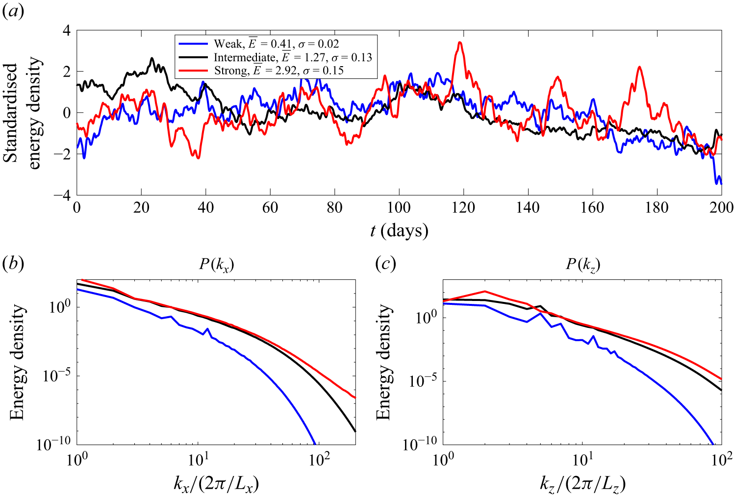
 P(kx)
 P(kz)
 0<|kx|/(2π/Lx)⩽2
 0<|kz|/(2π/Lz)⩽2
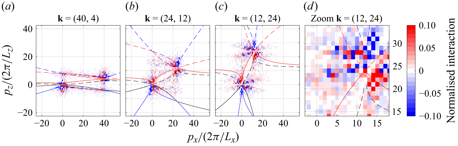
 Mabc(k,p,k−p)Ab,pAc,k−pAa,k∗
 k=(40,4)
 (24,12)
 (12,24)
 k
 k
 p∼k
 0<|kx|/(2π/Lx)⩽2
 0<|kz|/(2π/Lz)⩽2
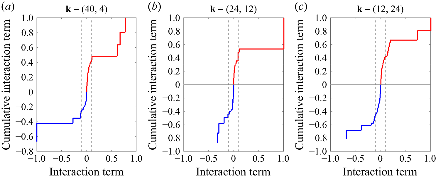
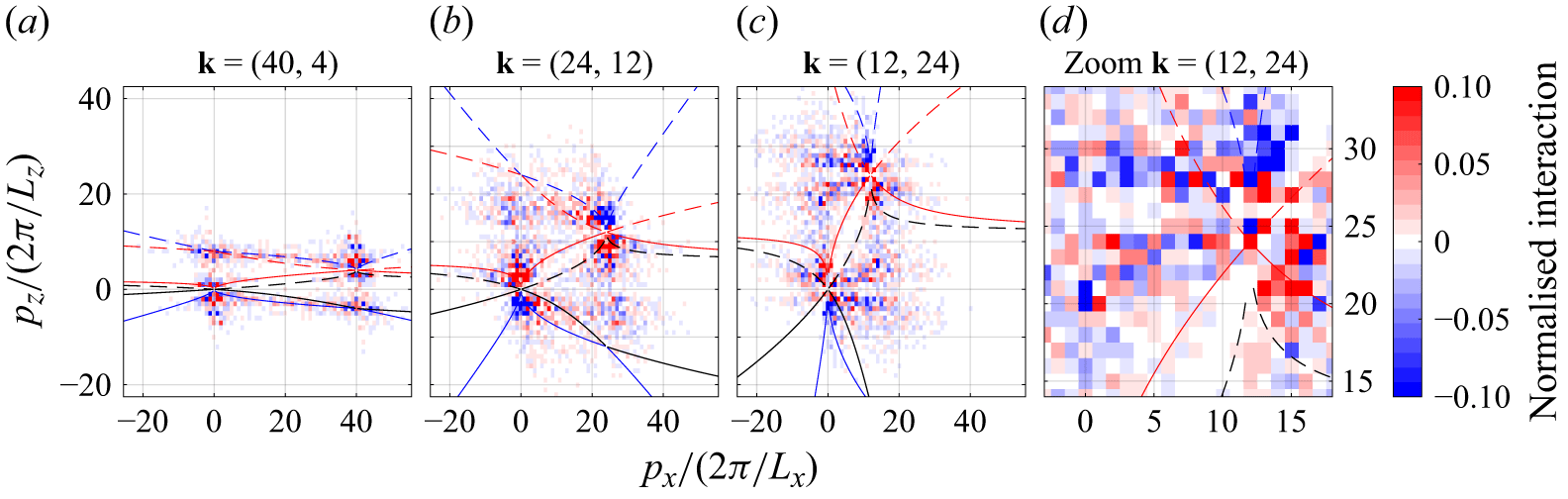
 k=(40,4),(24,12)
 (12,24)
 1024×512
 k
 p∼k
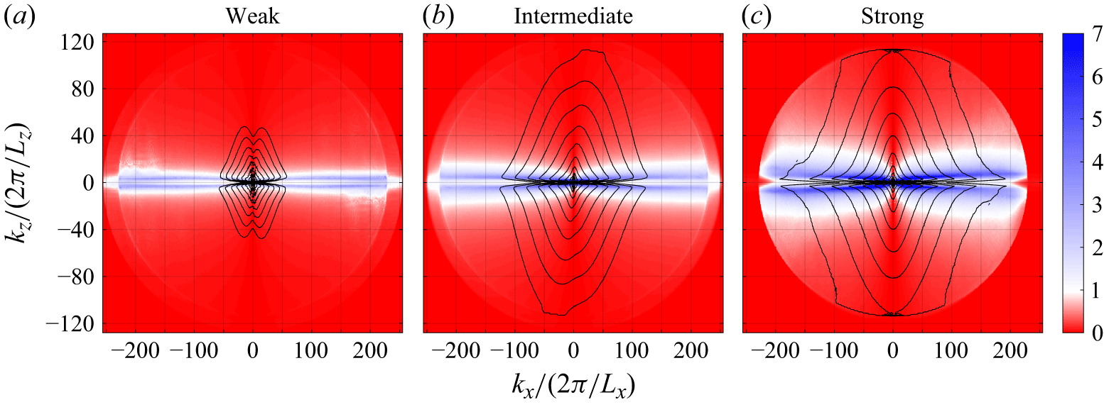
 V1≫1
 V1
 V1
 log10E(k)
 −8
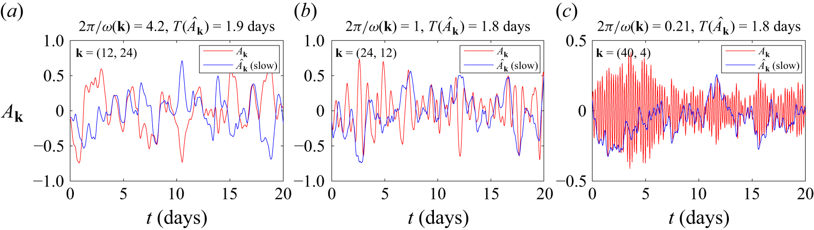
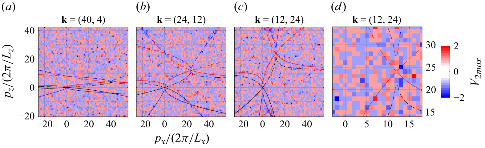
 V2


 Open access

