I. INTRODUCTION
A well-known figure of merit for a transmission link is the signal-to-noise-plus-intermodulation (IM) ratio (SNIR) or C/(N + I). It takes into account the transmitted power, link budget (gains and losses in the transmission path), and the receiver noise in carrier-to-noise ratio (C/N) combined with carrier-to-IM ratio (C/I) taking into account IM products created by non-linear power amplifiers. C/I ratio can be replaced by noise-power ratio (NPR) minus 1 as NPR is equivalent to (C + I)/I in the case of multicarrier transmission.
Interference from the same or other system also increases noise power and can be combined in a signal-to-noise-plus-IM-plus-interference ratio (SNIIR). In this paper, we consider either interference coming from different systems that will increase the receiver noise power by a constant value or interference coming from the same type of telecommunication system with power proportional to the carrier power giving a fixed carrier-to-interference ratio. We will first describe the case without interference and then derive both interference cases.
The C/(N + I) ratio is a useful factor of merit because it can be used to compute telecommunication system end-to-end performance such as bit-error rate (BER) in single or multicarrier telecommunication system using non-constant envelope digital modulation with or without error-correcting codes.
The main goal of the optimization criteria is to determine the single-carrier nominal power (P nom) and the operating point of the amplifier. The nominal power may be the n dB compression output power (P cn dB with n generally 1, 2, or 3) for a solid-state power amplifier (SSPA) or the saturated power (P sat) for a traveling wave tube amplifier (TWTA). It is related principally to the available technologies. The operating point is defined in terms of input or output back off (OBO) from the nominal power. For a given technology and nominal power, the operating point will define the C/I and the efficiency of the amplifier. Combined with the nominal power, it will define consumed power and dissipated power of the amplifier.
The oldest optimization criteria have been used to minimize the nominal power of the amplifier for a given C/(N + I) or maximize C/(N + I) for a given power, making the best use of the available technology.
Newer criteria have been proposed to minimize consumed power for a given C/(N + I), which is useful for both satellite payloads and handheld devices.
A criterion for the minimization of dissipated power is proposed in this paper together with a method for combining all criteria and determining the most useful specification changes. An example on the design of a broadcast satellite is given.
II. TRANSMISSION LINK AND DEFINITIONS
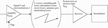
A typical transmission link scheme is given in Fig. 1. We define the transmit amplifier nominal output power P nom and consumed power P DC, the signal power C, the IM power I at amplifier output, the path losses L (including transmit and receive antennas gain and circuit losses), and the receiver input noise power N rec.
Transmission link scheme.

The signal-to-noise ratio (SNR) at receiver input is

In equation (1), we define N as the receiver noise referred to power amplifier output.
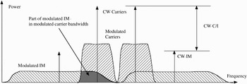
Signal power C at the output of non-linear transmit amplifier and received signal power C rec must be measured in the same conditions of modulation that will be used in the communication system and with the same receive filter. IM power I must also be measured in the same conditions; it is the total IM power at the output of the amplifier, in the useful signal bandwidth (with the same response as the receive filter). As can be seen on Fig. 2 comparing two CW and two modulated carriers, using the total IM power of CW carriers could give a large error as about one third of IM power falls into the carrier bandwidth.
We define the carrier-to-IM ratio in the carrier bandwidth as C/I. It can be combined with the carrier-to-noise ratio C/N in:

Measurement of pure carrier C/I and modulated carrier in-band C/I for two carriers.

We will use C/I throughout the paper but we could also use NPR − 1 where NPR is the noise power ratio, i.e. the ratio between signal plus noise and noise, measured in multicarrier operation (provided the same modulation conditions as in the real system are used).
In that case:

We can add interference either as a fixed noise at the receiver input, changing N to N + N int (e.g. industrial noise referred to amplifier output) or as a fixed ratio C/I int (e.g. adjacent system interference or lack of isolation between beams at the same frequency in the same system) in the combined SNIIR. Both types of interference may be present:

This formula can be derived easily in the optimization process from the SNIR formula by adding a fixed noise to the receiver noise and a fixed interference ratio or isolation ratio to the measured C/I.
We define the output operating point of the amplifier Ω as the ratio between the modulated carrier power output and the amplifier non-modulated single-carrier nominal power:

We express carrier power as a function of operating point:

The OBO is the reverse of the operating point. OBO is greater than 1 (positive in dB) when carrier power is lower than nominal power.
We define the input back-off (IBO or Φ) as the ratio between the amplifier non-modulated single-carrier input power corresponding to nominal output power P nom and the modulated carrier input power. OBO is a mathematical function of IBO: Ω(Φ), as there is only one value of OBO for any given IBO and for the given signal conditions. This function is different for each type of signal and modulation but always with Ω(0) = 0.
In the single-carrier case only, by definition: Ω(1) = 1. In general cases: Ω(1) ≤ 1.
We derive the following equations:

As C/I (or NPR) is also a function f of IBO, we define: C/I(Φ) = f(Φ) and we obtain:

III. NOMINAL POWER CRITERION
If our goal is to minimize nominal power for a given link budget, we observe that SNIR depends on parameter Ψ = P nom/N and not on both parameters P nom and N:

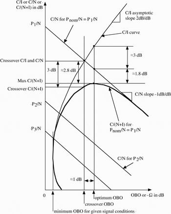
In Fig. 3, we draw a graph (in dB) of both terms in the sum as a function of OBO for different values of parameter Ψ. There is one curve for C/I with an asymptotic slope of 2 dB/dB and one straight line with slope −1 dB/dB for each value of parameter Ψ = P nom/N.
Graphical representation of combination of C/N and C/I.

We also draw the SNIR for one value of this parameter, (Ψ1 = P 1/N) and we determine its maximum.
We define the crossover point between C/I and C/N curves. SNIR is 3 dB lower than each element at the crossover point OBO.
For a C/I slope of 2 dB/dB and a C/N slope of −1 dB/dB, the C/(N + I) curve is in the form:

where x is the relative power with respect to the crossover point where C/I and C/N are equal.
The maximum of C/(N + I) is obtained for  corresponding to 1 dB lower power (or 1 dB more OBO) than the crossover point x = 1.
At this point, the corresponding C/I is 2 dB higher than the crossover and C/N is 1 dB lower thus giving a difference of 3 dB between C/I and C/N.
The maximum C/(N + I) is equal to the reciprocal of:  or 2.76 dB lower than the value of C/N or C/I at the crossover point.
Larger differences between C/I and C/N and between crossover and optimum C/(N + I) will be obtained at lower OBO where the C/I slope is much higher than 2 dB/dB (Fig. 3).
The optimization problem is then to find the lowest nominal power or parameter Ψ = P nom/N that will give the required SNIR.
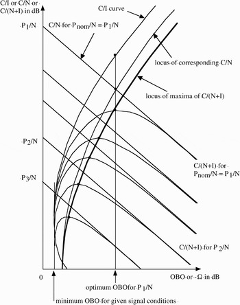
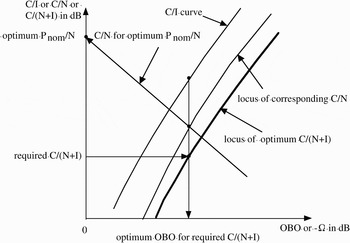
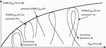
For this, we consider all possible values of this parameter and we draw a parametric set of SNIR curves in Fig. 4. Then we obtain the locus of maxima of these curves. Each point on this locus gives an optimum OBO for a given required SNIR (or conversely the maximum possible SNIR for a given OBO).
Locus of optimum OBO for required C/(N + I) and corresponding C/N and C/I.

As we also know the C/I for this OBO, we can draw the corresponding C/N locus, either by computing it from C/(N + I) and C/I or geometrically from the value of the C/N curve at optimum OBO.
Given such an abacus with C/I, optimum C/(N + I) and the corresponding C/N curves, we will draw a horizontal line at the required SNIR, then a vertical line through the point where this line crosses the optimum C/(N + I) locus. This will determine the optimum output operating point of the amplifier, OBO. This vertical line crosses the corresponding C/N locus and from this point a −1 dB/dB line to the vertical axis will give the lowest parameter Ψ = P nom/N that gives the required C/(N + I) (Fig. 5).
Use of the abacus to determine optimum OBO and nominal power.

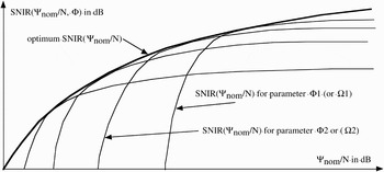
Another parametric representation could be obtained by drawing the set of SNIR curves as a function of Ψ = P nom/N, one curve for each value of input operating point Φ (Fig. 6).
Different graphical construction of the set of parametric curves.

Graph coordinates are:

In this type of graph, the optimum SNIR for a given nominal power or the minimum nominal power for a required SNIR is obtained directly from the envelope of the set of parametric curves. The operating point is obtained from the parameter of the curve in the set that is tangent to the envelope at the optimum point.
IV. DEMODULATION LOSS AND TOTAL DEGRADATION CRITERIA
The demodulation loss or SNR degradation, D has been defined in [Reference Casini, De Gaudenzi and Ginesi1] as the difference (in dB) between the required C/N to achieve the required SNIR and the C/N that would be required in a linear link. It is also the difference between the achieved SNIR with non-linear amplifier and the SNR or C/N that would be obtained from a linear link with same carrier power. In our graph D is the difference along the vertical axis between the optimum SNIR curve and the optimum C/N curve for a given operating point. It can be expressed also by:

The total RF degradation, TD has been defined as the sum of OBO (in signal and modulation conditions) and demodulation loss D.
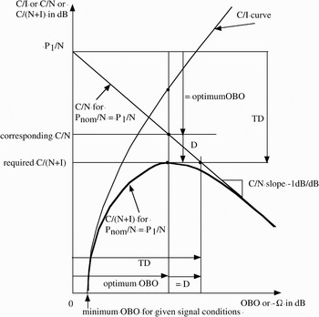
These two criteria are easily obtained on the graph in Fig. 7 that is derived from the one in Fig. 3.
Graphical construction of D and TD.

As the C/N curve has a slope of −1 dB/dB and crosses the vertical axis for which OBO = 0 at P 1/N, the distance between this point and the corresponding C/N is equal to the optimum OBO. The distance between corresponding C/N and required C/(N + I) is D from its definition. So, TD is the distance between P 1/N and required C/(N + I).
As the required C/(N + I) is on the maximum of the curve, TD is minimum in the same conditions where the saturated or nominal power is minimum.
Using a lower nominal power, we would not be able to achieve the required C/(N + I).
A higher power would achieve the required C/(N + I) for two possible operating points, each one with higher total degradation.
The main advantage of TD is that it is not necessary to compute the intermodulation noise falling in the carrier bandwidth as this is derived (if necessary) from the thermal noise ratio degradation (or from increase of this ratio necessary to get the same BER at the receiver and demodulator output).
Its drawback, however, is that in principle a measurement with the receiver and demodulator must be made for each operating point and value of thermal noise ratio.
One measurement of degradation of C/N by the non-linear amplifier can be used to verify that the computation of IM noise falling in the carrier bandwidth is correct thus validating the use of P nom/N criterion in a given experiment [Reference Anakabe2].
V. CONSUMED POWER CRITERION
The main drawback of the preceding criteria is that they do not take into account the efficiency of the amplifier.
To improve the classical criterion, we proposed to take into account in the optimization process the power consumed by the amplifier [Reference Sombrin3, Reference Sombrin4].
When measuring the amplifier, with the same signal and modulation conditions, using the same IBO definition, in addition to the output power and C/I or NPR, we measure the total consumed power relative to the nominal single-carrier output power. We obtain a function p:

For any link budget, using parameter Ψ = P nom/N that we already defined, we can reference the consumed power to the noise level reference at amplifier output:

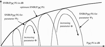
In the same manner as in Fig. 6, we draw a parametric set of curves given in Fig. 8, now with coordinates:

using one parameter Φ for each curve and varying parameter Ψ along each curve.
Graphical representation of C/(N + I) as a function of consumed power.

As in Fig. 6 we obtain an envelope for the set of curves from which we get the maximum SNIR for a given consumed power or the minimum consumed power for a required SNIR.
We do not use power efficiency in this paragraph but total consumed power because of the difficulty to define a meaningful efficiency for one modulated carrier in a multicarrier signal with respect to total consumed power.
As shown previously [Reference Sombrin3, Reference Sombrin4, Reference Aloisio, Casini and Ginesi5], this criterion will give an optimum point of operation at higher power than the P sat optimum because the optimum will move toward better efficiency.
VI. DC TOTAL DEGRADATION CRITERION
Consumed power is also taken into account in [Reference Aloisio, Casini and Ginesi5]. This is obtained by the DC total degradation TD(DC). This parameter takes into account the efficiency in the formula for total degradation TD thus giving the consumed power in the signal conditions instead of the RF power. This can be done for each value of required BER or signal to noise ratio at the input of the receiver. An optimum IBO is obtained when the DC total degradation is minimum. This optimum is shifted to lower IBO when compared to the TD case.
As in the case of comparison of TD and P nom/N criteria, the results of DC total degradation should be the same as the ones of P DC criteria if the same signal conditions are used.
The advantage and drawback with respect to P DC/N criterion are the same as for TD with respect to P nom/N criterion.
VII. DISSIPATED POWER CRITERION
In some cases, constraints on dissipated power may be more important than constraints on consumed power.
We can easily derive equivalent equations for dissipated power criterion by measuring this power as a function of IBO in the same conditions as the other curves:

As in Section V, we reference the dissipated power to the noise level reference at amplifier output:

In the same manner as in Figs 6 and 8, we draw a parametric set of curves, now with coordinates:

using one parameter Φ for each curve and varying parameter Ψ along each curve.
As in Figs 6 and 8 we obtain an envelope for the set of curves from which we get the maximum SNIR for a given dissipated power or the minimum dissipated power for a required SNIR (Fig. 9).
Graphical representation of C/(N + I) as a function of dissipated power.

As dissipated power is not a monotonous function of input power, parametric curves exhibit loops for negative slope (for low input power) or a singular point for null slope (when optimum point of operation is at minimum dissipated power).
Generally, we will measure the power dissipated by the amplifier but this can be applied to any power that is meaningful for technology or thermal design, such as:
• the power dissipated by the last stage of a solid-state amplifier;
• the power dissipated by the body of a TWTA with a radiating collector (because the power dissipated on the collector is directly radiated in space, whereas the body must be cooled by a radiator);
• the power dissipated by the amplifier and losses in an output circuit (because a radiator will be needed for this power).
If necessary, more than one such dissipation curve can be drawn and used in combination as will be shown in the next section.
VIII. CRITERIA COMBINATION
We will combine all criteria if we have more than one constraint to respect at the same time.
In the general case, we will work with margins that we will define for nominal power, consumed power, and dissipated power.
For each constraint on a given power (P sat max or P DC max or P diss max), we define a margin at the optimum point of operation as:

In equation (17), P x opt is the optimum power for the criterion that optimizes P x for the required SNIR and P x is one of P sat or P DC or P diss.
A positive margin (in dB) on any constraint is sufficient if we have only one constraint at a time.
However, if we have a combination of constraints, we must reference all margins to the same saturated power and operating point. For this, we note that if the required C/(N + I) or SNIR is fixed and as the C/I depends only on the operating point, we can compute the required C/N or SNR as a function of operating point only:

For a given SNIR and operating point, we have

We then compute margins for each constraint:

For comparison and combination, it will be easier to use relative margins, rm x, such as:

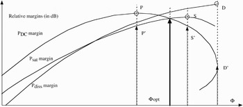
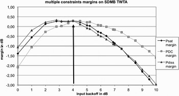
Figure 10 is an example of what can be obtained for these margins. Relative margin curves are drawn as a function of input operating point, Φ. They could be drawn as a function of OBO also. They are valid for one value of SNIR only.
Graphical representation of combination of three criteria (the first case).

On each curve the optimum point is either a maximum on the curve or at limit of validity domain. We indicate by three dots (S, P, and D) the optimum point for saturated, consumed, and dissipated power. For each of the three corresponding operating points we can see that the margin on one or both other curves is lower.
The combined margin is the minimum of all three margins. In this case, it has an optimum at the crossover point of saturated and consumed power margins.
This is a classical result in multiple constraints problems.
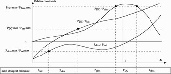
The points respecting two of the three constraints are given by one of the following equations:

The solutions in Φ for these equations are independent from the optimum points for each margin and can be computed beforehand. They depend only on the three given constraints.
Figure 11 gives a typical graph of these three equations and the solutions with the range in which each constraint is the more stringent.
Graphical representation of ranges of constraints.

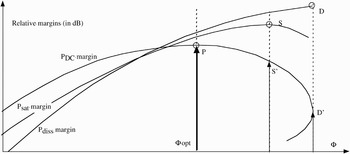
When one of the constraints is more stringent than the others, the combined optimum corresponds to its optimum. This is shown in Fig. 12.
Graphical representation of combination of three criteria (the second case).

IX. APPLICATION TO SDMB PAYLOAD OPTIMIZATION
This method has been applied to the SDMB project (S-band Direct Mobile Broadcasting), a satellite phase 0, and phase A study. These results were then used by industry to propose a mobile TV payload on a commercial satellite.
In this case, a total SNIIR of 5.5 dB was required in clear sky conditions to give adequate margins in rain and multipath conditions. Taking into account a given antenna isolation between spots C/I of 12 dB, the required SNIR (C over noise and IM) is 6.6 dB.
The graph in Fig. 13 is given for a maximum saturated power of 220 W, a maximum consumed power of 300 W and, a maximum dissipated power of 170 W. It is obtained from a 240 W TWTA measurement as a function of IBO (given in annex) and spacecraft performance. An initial solution was proposed with a saturated power of 220 W and an IBO of 4 dB.
Combination of three constraints for the measured SDMB TWTA.

Maximum consumed power and maximum dissipated power were specified as the ones expected on the 220 W TWTA at this operating point in multicarrier with a small margin.
The result of these choices is an over-constrained problem.
It was not possible, using lengthy link budget computation for each set of parameters to improve this initial solution because any change in one parameter would degrade the margin even when increasing either of the maximum values. Most of trial link budget computation would give a negative margin in one or other of the specifications.
From the graph, it is easy to understand the difficulty of optimization: the margin is low and all three constraints for the nominal link budget crossover at the same point, which is also at optimum or near the optimum for each constraint.
In addition, because of measurement errors and noise the curves are not smooth, this may induce numerical errors when searching for an optimum. The numerical problem could be improved by fitting smoother curves on the measured data but this could induce more errors.
The proposed method, by using multiple constraint optimization permitted to understand the problem and to propose a possible way out of the trap: increase the nominal power of TWTA and at the same time use direct radiating collectors to decrease dissipated power on the spacecraft radiator and use AsGa solar cells to increase consumed power margin. Any one or two of these three modifications would not increase the margin.
Applying the same computation to other values of required SNIIR or C/(N + I + IM) we could draw a graph of combined margin as a function of required SNIIR for any set of maximum power values.
X. SPECTRUM EFFICIENCY AND ENERGY CONSUMED PER BIT CRITERION
In addition to power efficiency, it is necessary for wireless systems to increase spectrum efficiency (the number of bits transmitted over a 1 Hz bandwidth) to improve the use of available spectrum.
A well-known barrier to better spectrum efficiency is the Shannon limit that gives the maximum capacity of a channel. Using the definitions in this paper, maximum spectrum efficiency is:

This value is obtained when the channel bandwidth is equal to the symbol rate and the noise-plus-interference power is measured in the same bandwidth, which is the noise bandwidth of the optimum receiver.
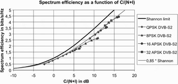
Receivers exhibit implementation losses and their spectrum efficiency is lower than the Shannon limit. Figure 14 gives the theoretical limit, curves for coding and modulation schemes used in DVB-S2 standard and an empirical approximation of the degradation due to implementation.
Spectrum efficiency as a function of C/(N + I) for the Shannon limit and DVBS2 standard demodulator curves.

We find that these receivers operate at nearly 85% of the Shannon limit in a wide range of SNIR when the transmission link knows or evaluate the SNIR and adapts the coding and modulation scheme that is used.
DVB-S2 curves are given for each modulation scheme and points on the curves are given for each coding scheme.
In addition, it must be noted that the signal occupies a bandwidth higher than the symbol rate because the roll-off coefficient of 10–35% must be taken into account and microwave filters will have guard bands around 10%.
This gives an overall spectrum efficiency of 70–57% of the Shannon limit.
We note that for such a transmission link the required SNIR may be very low as the minimum value for the link is −2.5 dB in this example. Strongly non-linear amplifiers can be used at operating points near optimum efficiency giving an NPR around 10 dB.
A more stringent constraint will be a minimum spectrum efficiency that will be required to insure a required link capacity on a given available bandwidth. This will directly drive the energy consumed per bit for a given modulation and a coding scheme. Multiplying this value by the required capacity in bits/s will give the minimum consumed power.
In the previous optimization graphs, we can easily transform the vertical axis, SNIR to spectral efficiency by using the Shannon limit or a percentage of this limit or any real demodulator curve.
This will give graphs of optimum spectrum efficiency as a function of the horizontal axes values (e.g. P DC/N, P nom/N, or P diss/N).
A more interesting graph is obtained if we use for the horizontal axis the power variable divided by the spectrum efficiency as this will give us access to an energy per bit, e.g. saturated energy per bit, consumed energy per bit, or dissipated energy per bit [Reference Sombrin6].
As an example, with consumed power, we have:

In this equation, E DC is the energy that is consumed by the amplifier for the transmission of each bit and No is the thermal noise power spectral density (referred to power amplifier output).
It is related broadly to the well-known energy per bit through the power efficiency at the operating point of the amplifier:

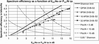
The corresponding graph is given in Fig. 15. Three curves have been added for typical values of P DC/N, only the part under the Shannon limit can be used.
Spectrum efficiency as a function of energy consumed per bit of a linearized TWTA for the Shannon limit and DVB-S2 standard demodulator curves.

As can be seen on the graph, the change in P DC/N is quite higher than the corresponding change in E DC/No for these demodulator curves (10 dB compared to 5 dB).
This criterion will be of great interest for all cases where the available energy is limited, e.g. deep space satellites, hand-held devices, and RFID devices.
As an example, for a 1 b/s spectrum efficiency we need a C/(N + I), an Eb/No of 1 dB, and an E DC/No of 4.25 dB giving a power efficiency of 47%.
For 3 b/s, this optimization will result in a power efficiency of 23% for a C/(N + I) of 10 dB. This is quite interesting in a system that is more bandwidth limited than energy limited. Keeping the same capacity, by doubling the consumed energy per bit, it is possible to divide the used bandwidth by 3.
We can see also that the most robust modulation and coding scheme consumes more energy per bit and has a lower spectrum efficiency than the next scheme; so it should not be used.
The same derivation can be applied to saturated or nominal power giving directly saturated or nominal amplifier energy per bit E nom/No and eventually for dissipated power.
XI. CONCLUSION
Starting from the well-known figures of merit such as SNIR or C/(N + I) and total degradation TD, which are equivalent to a minimum nominal power criterion, we have introduced more advanced criteria such as minimum consumed power or dissipated power.
We proposed a method to combine criteria in a multiple constraints optimization.
This was applied to measurements of a linearized TWTA in the case of SDMB project.
Finally, we combine the criteria with the Shannon theoretical limit and some practical demodulator curves to obtain optimum values for energy consumed or dissipated for each bit transmitted through a non-linear link as a function of the link noise power spectral density.
These last criteria could be used for energy-limited equipments such as in deep space satellites, hand-held devices, or RFID devices.
APPENDIX
A. MODEL OF TWTA USED
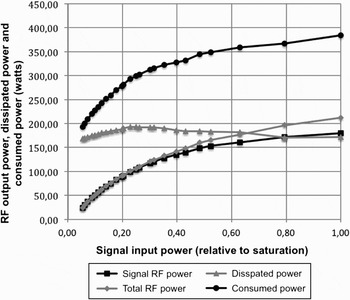
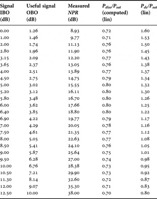
Measurements of a 240-W linearized TWTA have been used to model the performance of a 220-W linearized TWTA (see table 1 and Fig 16).
RF signal output power, total RF output power, dissipated power, and consumed power as the function of input power relative to saturation.

Measured values of 240-W linearized TWTA.

Measured NPR is of the form (C + I)/I.
Dissipated power was computed as consumed power minus total RF output power.
Total RF output power is the sum of useful signal output power and intermodulation output power.
 Jacques B. Sombrin received his engineering diplomas from Ecole Polytechnique, Paris, in 1972 and from Ecole Nationale Supérieure des Télécommunications, Paris, in 1974. He worked then in the microwaves domain. He is now assistant director for Radio Frequencies in CNES, the French Space Agency. His main research interests are simulation of non-linear behavior of transmission equipments and optimization of non-linear microwave power amplifiers used in satellites.