1 Introduction
For a Newtonian fluid, the constitutive model governing the relationship between the viscous stresses
 $\unicode[STIX]{x1D70F}_{ij}$
and the strain rates is expressed:
 $$\begin{eqnarray}\unicode[STIX]{x1D70F}_{ij}=\unicode[STIX]{x1D707}\left(\frac{\unicode[STIX]{x2202}u_{i}}{\unicode[STIX]{x2202}x_{j}}+\frac{\unicode[STIX]{x2202}u_{j}}{\unicode[STIX]{x2202}x_{i}}-\frac{2}{3}\unicode[STIX]{x0394}\unicode[STIX]{x1D6FF}_{ij}\right)+\unicode[STIX]{x1D707}_{b}\unicode[STIX]{x0394}\unicode[STIX]{x1D6FF}_{ij},\end{eqnarray}$$
where
 $u_{i}$
is the velocity vector,
 $\unicode[STIX]{x0394}=\unicode[STIX]{x2202}u_{k}/\unicode[STIX]{x2202}x_{k}$
the dilatation (rate),
 $\unicode[STIX]{x1D6FF}_{ij}$
the identity tensor,
 $\unicode[STIX]{x1D707}$
the shear viscosity and
 $\unicode[STIX]{x1D707}_{b}$
the bulk viscosity. The expression in parentheses is deviatoric, while the last term accounts for volumetric changes. Bulk viscosity, sometimes called dilatational, volumetric or second viscosity, evidently is a proportionality constant between the isotropic part of the viscous stress and dilatation rate. The corresponding viscous dissipation rate
 $\unicode[STIX]{x1D6F7}$
, including shear and dilatational contributions, can be written (Lele Reference Lele1994):
 $$\begin{eqnarray}\unicode[STIX]{x1D6F7}=\unicode[STIX]{x1D70F}_{ij}\unicode[STIX]{x1D61A}_{ij}=2\unicode[STIX]{x1D707}\unicode[STIX]{x1D61A}_{ij}^{(d)}\unicode[STIX]{x1D61A}_{ij}^{(d)}+\unicode[STIX]{x1D707}_{b}\unicode[STIX]{x1D6E5}^{2},\end{eqnarray}$$
where
 $\unicode[STIX]{x1D61A}_{ij}=(\unicode[STIX]{x2202}u_{i}/\unicode[STIX]{x2202}x_{j}+\unicode[STIX]{x2202}u_{j}/\unicode[STIX]{x2202}x_{i})/2$
is the strain rate tensor and
 $\unicode[STIX]{x1D61A}_{ij}^{(d)}=\unicode[STIX]{x1D61A}_{ij}-\unicode[STIX]{x0394}\unicode[STIX]{x1D6FF}_{ij}/3$
is its deviatoric part. Equation (1.2) indicates that the two parameters of importance to assess the importance of bulk viscosity on turbulent kinetic energy dissipation are the bulk to shear viscosity ratio,
 $\unicode[STIX]{x1D707}_{b}/\unicode[STIX]{x1D707}$
, and the ratio of the square of the volumetric to deviatoric deformation rates,
 $\unicode[STIX]{x1D6E5}^{2}/\unicode[STIX]{x1D61A}_{ij}^{(d)}\unicode[STIX]{x1D61A}_{ij}^{(d)}$
. The former is an input parameter dependent on the fluid, while the latter an output of the calculation.
As noted by Graves & Argrow (Reference Graves and Argrow1999), bulk viscosity is routinely set to zero in a variety of fluid mechanics studies by invoking Stokes’ hypothesis (Stokes Reference Stokes1851). This assumption is justified if
 $\unicode[STIX]{x1D707}_{b}=0$
or/and
 $\unicode[STIX]{x1D6E5}=0$
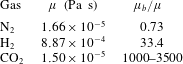
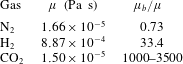
. Only dilute monatomic gases have zero bulk viscosity. For polyatomic gases, experimental measurements indicate that bulk viscosity can be substantially greater than its shear counterpart (table 1); for
 $\text{CO}_{2}$
, it can be thousands of times larger, in which case the role of dilatational losses on turbulence decay is expected to be magnified, depending on the relative importance of volumetric to deviatoric deformations. Although dilatational dissipation is often small compared to its shear counterpart in weakly compressible flows, numerous studies highlight the importance of dilatational effects in analysis and modelling of compressible turbulence (Sarkar et al.
Reference Sarkar, Erlebacher, Hussaini and Kreiss1991; Kida & Orszag Reference Kida and Orszag1992; Lele Reference Lele1994; Pirozzoli & Grasso Reference Pirozzoli and Grasso2004).
Shear viscosity and bulk to shear viscosity ratio at room temperature for different gases (Tisza Reference Tisza1942; Emanuel Reference Emanuel1990; Billet, Giovangigli & de Gassowski Reference Billet, Giovangigli and de Gassowski2008; Cramer Reference Cramer2012).
The manifestation of these volumetric effects can be illustrated by decomposing the (total) stress tensor
 $\unicode[STIX]{x1D748}$
into isotropic and deviatoric terms,
 $$\begin{eqnarray}\unicode[STIX]{x1D70E}_{ij}=-p\unicode[STIX]{x1D6FF}_{ij}+2\unicode[STIX]{x1D707}\unicode[STIX]{x1D61A}_{ij}^{(d)}+\unicode[STIX]{x1D707}_{b}\unicode[STIX]{x0394}\unicode[STIX]{x1D6FF}_{ij},\end{eqnarray}$$
where
 $p$
is the static pressure of the gas at rest under the same thermodynamic conditions (i.e. same composition, density, temperature and internal energy). The mechanical pressure,
 $\bar{p}=-\unicode[STIX]{x1D70E}_{ii}/3$
, can then be expressed:
 $$\begin{eqnarray}\bar{p}=p-\unicode[STIX]{x1D707}_{b}\unicode[STIX]{x1D6E5}.\end{eqnarray}$$
In the presence of large changes in density produced by the flow, the mechanical pressure
 $\bar{p}$
departs from the thermodynamic pressure
 $p$
corresponding to local thermodynamic equilibrium (LTE) conditions.
While mechanical pressure corresponds to the translational energy of molecules, thermodynamic pressure is a measure of the total energy and includes internal (vibrational and rotational) degrees of freedom, in addition to translational. When rapid changes in the thermodynamic state are caused by the flow, the fluid is no longer in equilibrium, thus prompting internal processes to drive the state toward equilibrium (Landau & Lifshitz Reference Landau and Lifshitz1987); in dilute polyatomic gases for instance, these processes are caused by inelastic collisions between internal degrees of freedom (Hirschfelder et al.
Reference Hirschfelder, Curtiss, Bird and Mayer1954; Vincenti & Kruger Reference Vincenti and Kruger1965; Emanuel Reference Emanuel1990). The deviation between mechanical and thermodynamic pressures is a direct consequence of a relaxation process seeking to achieve equipartition of energy. This relaxation gives rise to reduced mechanical pressure in an expanding flow (
 $\bar{p}<p$
) and increased mechanical pressure under compression (
 $\bar{p}>p$
). In other words, bulk viscosity is a description of non-equilibrium energy transfer between translational and internal (vibrational and rotational) degrees of freedom. It further follows that the rate at which the isotropic part of the stress tensor does work (per unit volume) is (Batchelor Reference Batchelor1968):
 $$\begin{eqnarray}-\bar{p}\unicode[STIX]{x1D6E5}=-p\unicode[STIX]{x1D6E5}+\unicode[STIX]{x1D707}_{b}\unicode[STIX]{x1D6E5}^{2}.\end{eqnarray}$$
The first term on the right-hand side is (reversible) work done by thermodynamic pressure. The second term, the same as in (1.2), is positive and represents mechanical energy dissipation. Equations (1.4) and (1.5) illustrate that bulk viscosity is a continuum construct attempting to describe complex relaxation phenomena occurring at the molecular level, which dissipate energy through volumetric motions.
The idea of a bulk viscosity has been questioned over the years (Vincenti & Kruger Reference Vincenti and Kruger1965; Batchelor Reference Batchelor1968; Ern & Giovangigli Reference Ern and Giovangigli1996; Meador, Miner & Townsend Reference Meador, Miner and Townsend1996; Giovangigli Reference Giovangigli1999). Its incorporation into the Navier–Stokes equations following (1.1) is valid only for small deviations from LTE (Vincenti & Kruger Reference Vincenti and Kruger1965). For gases with large bulk-to-shear viscosity ratio, the characteristic non-equilibrium time scale is of the order of microseconds (Konyukhov, Korogod & Tikhonov Reference Konyukhov, Korogod and Tikhonov1969) at room temperature, such that LTE is a valid approximation for many problems. For substantial departures from LTE, the energy transfer between modes should be addressed using more sophisticated approaches, e.g. non-equilibrium rate equations (Graves & Argrow Reference Graves and Argrow1999). Although numerical estimates can be made for bulk viscosity (Cramer Reference Cramer2012), quantitative experimental measurements are challenging (Emanuel Reference Emanuel1990). Attempts to measure bulk viscosity are often made acoustically (Landau & Lifshitz Reference Landau and Lifshitz1987; Graves & Argrow Reference Graves and Argrow1999), in which case there is a clear frequency dependence, as expected since the magnitude of
 $\unicode[STIX]{x1D707}_{b}$
depends on the relative magnitude of the characteristic time of the dilatational process (via the flow) to the relaxation time. These measurements suggest that bulk viscosity is likely to affect compressible flows with broadband motions, such as acoustics or turbulence.
The influence of bulk viscous dissipation on fluid dynamics has been investigated in the context of certain engineering applications. Aerodynamic heating during Mars entry, where the atmosphere primarily consists of carbon dioxide, provides a motivation for understanding flows in which bulk viscosity is large (Emanuel Reference Emanuel1990). Early studies (Emanuel Reference Emanuel1992; Gonzalez & Emanuel Reference Gonzalez and Emanuel1993) evaluated the effects of bulk viscosity on heat transfer in laminar Couette and hypersonic boundary layer flows. In combustion, Billet et al. (Reference Billet, Giovangigli and de Gassowski2008) numerically simulated the interaction of a planar shock with a hydrogen bubble; they found that flow features such as pressure gradients and baroclinic vorticity production depend on bulk viscosity. Fru, Janiga & Thévenin (Reference Fru, Janiga and Thévenin2011) further demonstrated using direct numerical simulation (DNS) that laminar flames exhibit little sensitivity to
 $\unicode[STIX]{x1D707}_{b}$
, but that turbulence amplifies small instantaneous discrepancies originating from bulk viscous effects, thus leading to different flow evolution and flame structure. Bahmani & Cramer (Reference Bahmani and Cramer2014) simulated a two-dimensional shock–boundary-layer interaction with varying bulk viscosity. They found that shock-induced separation is suppressed in calculations with bulk viscosity due to thickening of the incident shock and subsequent reduction of the adverse pressure gradient magnitude. At high Reynolds number, bulk viscosity gives rise to a variation of the thermodynamic pressure across the boundary layer via source terms in the energy equation (Bahmani & Cramer Reference Bahmani and Cramer2014; Cramer & Bahmani Reference Cramer and Bahmani2014). Recent years have seen the emergence of gas-kinetic schemes (GKS, Liao, Peng & Luo Reference Liao, Peng and Luo2009, Reference Liao, Peng and Luo2010; Kumar, Girimaji & Kerimo Reference Kumar, Girimaji and Kerimo2013), into which bulk viscous dissipation is generally built, to simulate compressible turbulence. In a specific study of bulk viscosity using GKS, Liao et al. (Reference Liao, Peng and Luo2009) found that dilatational dissipation is increased when bulk viscosity is included, and that skewness and flatness are modified at turbulent Mach numbers of 0.5, although the detailed mechanisms are not fully explained.
While questions remain on how to accurately represent bulk viscosity in continuum calculations of polyatomic gases, there is a need to understand the effects of bulk viscosity on flows with broadband motions. For instance, it is questionable whether, for sufficiently compressible turbulence and gases with large
 $\unicode[STIX]{x1D707}_{b}/\unicode[STIX]{x1D707}$
such as
 $\text{CO}_{2}$
, bulk viscosity can readily be neglected. The objective of this study is to quantitatively understand the mechanisms by which bulk viscosity and its associated phenomena affect the dynamics and energy transfer of compressible turbulence. Equation (1.2) indicates that turbulent kinetic energy dissipation depends on the bulk to shear viscosity ratio and the ratio of the square of the volumetric to deviatoric deformation rates; our focus solely lies in isolating the effect of the former. For this purpose, we use DNS to simulate the decay of compressible, homogeneous, isotropic turbulence for ratios of bulk-to-shear viscosity between 0–1000 and moderate compressibility (no eddy shocklets). Following the assumption made by Bahmani & Cramer (Reference Bahmani and Cramer2014), we assign a constant value to bulk viscosity, i.e. LTE conditions are assumed such that
 $\unicode[STIX]{x1D707}_{b}$
is a (frequency-independent) constant. This assumption is valid as long as LTE holds, i.e. as long as the Kolmogorov (time) scale is much larger than the internal molecular non-equilibrium time scale. Given the form of (1.1), we hypothesize that bulk viscosity will increase compressible damping; in particular, we seek to determine its effect on dilatational versus solenoidal motions. Organization-wise, we first describe the governing equations and the set-up of the problem under consideration, including the initial conditions. After investigating the evolution of mean quantities to highlight the key contributions of bulk viscosity, we focus on budgets to explain energy transfer, for which we rely on a Helmholtz decomposition of the velocity field. Next, we analyse the spectral content, and resulting probability density functions, before finally considering turbulent Mach number dependence.
2 Problem formulation
2.1 Equations of motion and numerical method
The objective of this study is to understand the mechanisms by which phenomena associated with the presence of bulk viscosity affect compressible turbulence. For this purpose, we use direct numerical simulation, in which all dynamical scales of motion are resolved. The compressible Navier–Stokes equations for a perfect gas describe the problem under consideration, written here is non-dimensional form:
 $$\begin{eqnarray}\displaystyle & \displaystyle \frac{\unicode[STIX]{x2202}\unicode[STIX]{x1D70C}}{\unicode[STIX]{x2202}t}+\frac{\unicode[STIX]{x2202}}{\unicode[STIX]{x2202}x_{j}}(\unicode[STIX]{x1D70C}u_{j})=0, & \displaystyle\end{eqnarray}$$
 $$\begin{eqnarray}\displaystyle & \displaystyle \frac{\unicode[STIX]{x2202}(\unicode[STIX]{x1D70C}u_{i})}{\unicode[STIX]{x2202}t}+\frac{\unicode[STIX]{x2202}}{\unicode[STIX]{x2202}x_{j}}(\unicode[STIX]{x1D70C}u_{i}u_{j}+p\unicode[STIX]{x1D6FF}_{ij})=\frac{1}{Re}\frac{\unicode[STIX]{x2202}\unicode[STIX]{x1D70F}_{ij}}{\unicode[STIX]{x2202}x_{j}}, & \displaystyle\end{eqnarray}$$
 $$\begin{eqnarray}\displaystyle & \displaystyle \frac{\unicode[STIX]{x2202}E}{\unicode[STIX]{x2202}t}+\frac{\unicode[STIX]{x2202}}{\unicode[STIX]{x2202}x_{j}}[u_{j}(E+p)]=\frac{\unicode[STIX]{x2202}}{\unicode[STIX]{x2202}x_{j}}(u_{i}\unicode[STIX]{x1D70F}_{ij})+\frac{1}{Re\,Pr}\frac{\unicode[STIX]{x2202}^{2}T}{\unicode[STIX]{x2202}x_{j}^{2}}, & \displaystyle\end{eqnarray}$$
where
 $\unicode[STIX]{x1D70C}$
is the density,
 $Re=\unicode[STIX]{x1D70C}_{r}u_{r}L/\unicode[STIX]{x1D707}$
the Reynolds number,
 $Pr=\unicode[STIX]{x1D707}/(\unicode[STIX]{x1D70C}\unicode[STIX]{x1D6FC})=0.7$
the Prandtl number,
 $\unicode[STIX]{x1D6FC}$
the thermal diffusivity,
 $E=p/(\unicode[STIX]{x1D6FE}-1)+\unicode[STIX]{x1D70C}u^{2}/2$
the total energy and
 $T$
the temperature. Non-dimensionalization is performed using reference velocity
 $u_{r}$
, density
 $\unicode[STIX]{x1D70C}_{r}$
and length
 $L_{r}$
. The viscosities and thermal diffusivity are assumed constant, with no temperature or frequency dependence. As described by Bahmani & Cramer (Reference Bahmani and Cramer2014) and Cramer & Bahmani (Reference Cramer and Bahmani2014), this physical model adequately describes compressible turbulence with bulk viscous dissipation as long as the system is not too far from local thermodynamic equilibrium, which we assume to hold here. Given the parameters governing our problem, LTE can be ensured by prescribing a sufficiently high pressure.
We use a high-order accurate, explicit finite-difference approach, previously leveraged for DNS of turbulent multi-material mixing (Movahed & Johnsen Reference Movahed and Johnsen2015). In the problem under consideration, the flow is sufficiently smooth (i.e. the turbulent Mach number is low enough) that no shock capturing is required. We use sixth-order explicit central differences in the split form for the convective terms. The flux of Ducros et al. (Reference Ducros, Laporte, Souleres, Guinot, Moinat and Caruelle2000) in the form of Blaisdell (Reference Blaisdell1991) is used, following the generalization of Pirozzoli (Reference Pirozzoli2010),
 $$\begin{eqnarray}\frac{\unicode[STIX]{x2202}(\unicode[STIX]{x1D70C}u\unicode[STIX]{x1D719})}{\unicode[STIX]{x2202}x}=\frac{1}{2}\left[\frac{\unicode[STIX]{x2202}(\unicode[STIX]{x1D70C}u\unicode[STIX]{x1D719})}{\unicode[STIX]{x2202}x}+\unicode[STIX]{x1D719}\frac{\unicode[STIX]{x2202}(\unicode[STIX]{x1D70C}u)}{\unicode[STIX]{x2202}x}+\unicode[STIX]{x1D70C}u\frac{\unicode[STIX]{x2202}\unicode[STIX]{x1D719}}{\unicode[STIX]{x2202}x}\right],\end{eqnarray}$$
where
 $\unicode[STIX]{x1D719}$
is
 $(1,u_{i},(E+p)/\unicode[STIX]{x1D70C})$
. Standard sixth-order central differences are used for the diffusion terms, and time marching is handled using an explicit third-order strong stability preserving Runge–Kutta scheme (Gottlieb, Shu & Tadmor Reference Gottlieb, Shu and Tadmor2001).
2.2 Problem set-up
DNS (Moin & Mahesh Reference Moin and Mahesh1998) has enabled important advances in our understanding of compressible turbulence (Sarkar Reference Sarkar1992; Huang, Coleman & Bradshaw Reference Huang, Coleman and Bradshaw1995; Vreman, Sandham & Luo Reference Vreman, Sandham and Luo1996; Pirozzoli, Grasso & Gatski Reference Pirozzoli, Grasso and Gatski2004; Larsson & Lele Reference Larsson and Lele2009). Recently, various non-equilibrium effects have been included in computational investigations (Livescu, Jaberi & Madnia Reference Livescu, Jaberi and Madnia2002; Lee, Girimaji & Kerimo Reference Lee, Girimaji and Kerimo2009; Donzis & Maqui Reference Donzis and Maqui2016). In studies of the decay of compressible, homogeneous, isotropic turbulence, the conventional approach is to initially prescribe a random, often divergence-free, velocity field with given intensity and spectrum, e.g. following Rogallo (Reference Rogallo1981). Corresponding initial pressure and density fluctuations can be computed from the velocity field (Feiereisen Reference Feiereisen1981; Ristorcelli & Blaisdell Reference Ristorcelli and Blaisdell1997) but do not substantially influence the turbulence statistics (Samtaney, Pullin & Kosovic Reference Samtaney, Pullin and Kosovic2001). Details on generating this initial field can be found in other works (Blaisdell Reference Blaisdell1991; Johnsen et al.
Reference Johnsen, Larsson, Bhagatwala, Cabot, Moin, Olson, Rawat, Shankar, Sjögreen and Yee2010). Although originally intended for incompressible turbulence, this approach has been used to simulate compressible turbulence (Lee, Lele & Moin Reference Lee, Lele and Moin1991) and, in this context, has two main disadvantages. The first is that the random field evolves to an equilibrium turbulent state over approximately two eddy-turnover times, over which the energy is redistributed across scales to achieve the expected inertial range and a state of turbulence. This process is evident in the time evolution of enstrophy, which first increases due to vortex stretching before reaching a maximum and decreasing (see for instance figure 1 in Movahed & Johnsen Reference Movahed and Johnsen2015). Thus, if bulk viscosity were to be introduced from the beginning, the study would be one of the effect of bulk viscosity on this artificial transient rather than on decaying turbulence. Our remedy is to let the initial random field evolve beyond this transient with
 $\unicode[STIX]{x1D707}_{b}=0$
, and then introduce bulk viscosity. Although the flow still needs to adjust, this process occurs within a tenth of an eddy-turnover time. An alternative would be to sample from forced turbulence (Kida & Orszag Reference Kida and Orszag1992), but such a procedure generally results in non-physical behaviour at low wavenumbers. The second disadvantage is related to our hypothesis, which we verify in this study, that bulk viscosity affects dilatational and solenoidal motions to different extents. Following the conventional approach to generate initial conditions, acoustic and entropy modes are produced because the flow is not in acoustic equilibrium, and subsequently interact with vortical modes (Kovasznay Reference Kovasznay1988). The resulting flow is only slightly dilatational due to the relatively low Mach number. With this procedure, the magnitude of the dilatational intensity cannot be controlled independently of the solenoidal intensity of the turbulence. Our remedy is to decompose the initial velocity into solenoidal and dilatational components and prescribe each one separately, to precisely control the relative dilatational vs. solenoidal turbulence intensity.
Our initial conditions are generated to (i) discriminate between solenoidal and dilatational velocity contributions, and (ii) bypass the initial transition period generally produced by conventional approaches. We first address (i). Since past studies showed that the initial pressure and density fluctuations do not significantly affect the turbulence statistics, we set these to zero. Inspired by the approach of Pirozzoli & Grasso (Reference Pirozzoli and Grasso2004) to distinguish between dilatational and solenoidal motions, we perform a Helmholtz decomposition on the square root of the density-weighted velocity (Kida & Orszag Reference Kida and Orszag1992):
 $$\begin{eqnarray}w_{i}=\sqrt{\unicode[STIX]{x1D70C}}u_{i}=w_{i}^{(d)}+w_{i}^{(s)},\end{eqnarray}$$
where the
 $d$
and
 $s$
superscripts denote dilatational and solenoidal, respectively, with
 $\unicode[STIX]{x2202}w_{k}^{(s)}/\unicode[STIX]{x2202}x_{k}=0$
and
 $\unicode[STIX]{x1D735}\times \boldsymbol{w}^{(d)}=0$
. Given this velocity decomposition, we create two (different) random fields in wavenumber space, with each spectrum proportional to
 $k^{4}\exp (-2k^{2}/k_{0}^{2})$
, where
 $k$
is the wavenumber and
 $k_{0}$
the most energetic wavenumber (Lee et al.
Reference Lee, Lele and Moin1991). Upon transformation into physical space, one field corresponds to
 $w_{i}^{(s)}$
, the other to
 $w_{i}^{(d)}$
. In physical space, the fields are scaled to achieve the desired turbulence intensity. This procedure allows us to control solenoidal and dilatational velocity components independently of each other. We evaluated different ratios of initial dilatational to solenoidal root-mean-squared velocity
 $u_{rms}$
and found that the results exhibited little sensitivity to the relative magnitude of the dilatational to solenoidal contribution for factors ranging from
 $1/2$
to
 $3/2$
; for purely solenoidal initial conditions however, they did (e.g. quantitative difference in turbulent kinetic energy versus time). For simplicity, we set the intensity of the dilatational component equal to that of the solenoidal component. To address (ii), we evolve the initial random field for three eddy-turnover times with zero bulk viscosity, at which point a state of turbulence has been achieved. We consider this state to be our time origin and introduce the desired bulk viscosity.
The problem is initialized as follows. We consider a
 $(2\unicode[STIX]{x03C0})^{3}$
cube with periodic boundary conditions;
 $k_{0}=4$
defines the initial Taylor scale
 $\unicode[STIX]{x1D706}_{0}=2/k_{0}$
. Initially 180, the Taylor-based Reynolds number
 $Re_{\unicode[STIX]{x1D706}}$
defines the initial
 $u_{rms}$
and reaches 54 after three eddy-turnover times (i.e. our time origin); the eddy-turnover time is
 $\unicode[STIX]{x1D70F}=\unicode[STIX]{x1D706}_{0}/u_{rms,0}$
. For such values of
 $Re_{\unicode[STIX]{x1D706}}$
, we recognize that the results may exhibit Reynolds number dependence; given the finite computational resources, we chose the largest initial Reynolds number that would still enable varying parameters of interest (bulk viscosity ratio). Initially 0.1, the turbulent Mach number
 $M_{t}$
is sufficiently small that no eddy shocklets are produced. Thus, shock capturing, which would introduce numerical dissipation difficult to distinguish from physical dissipation, is not required; we further remark that generally weak shocklets could be resolved on a sufficiently fine grid, but at the expense of a greater computational cost. After
 $3\unicode[STIX]{x1D70F}$
,
 $M_{t}$
reaches approximately 0.065; we consider different initial turbulent Mach numbers in § 3.5 only. The parameter of interest is the ratio of bulk to shear viscosities,
 $\unicode[STIX]{x1D707}_{b}/\unicode[STIX]{x1D707}$
, which we set to zero (Stokes’ hypothesis), 30 (corresponding to
 $\text{H}_{2}$
) and 1000 (corresponding to
 $\text{CO}_{2}$
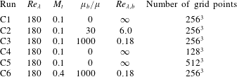
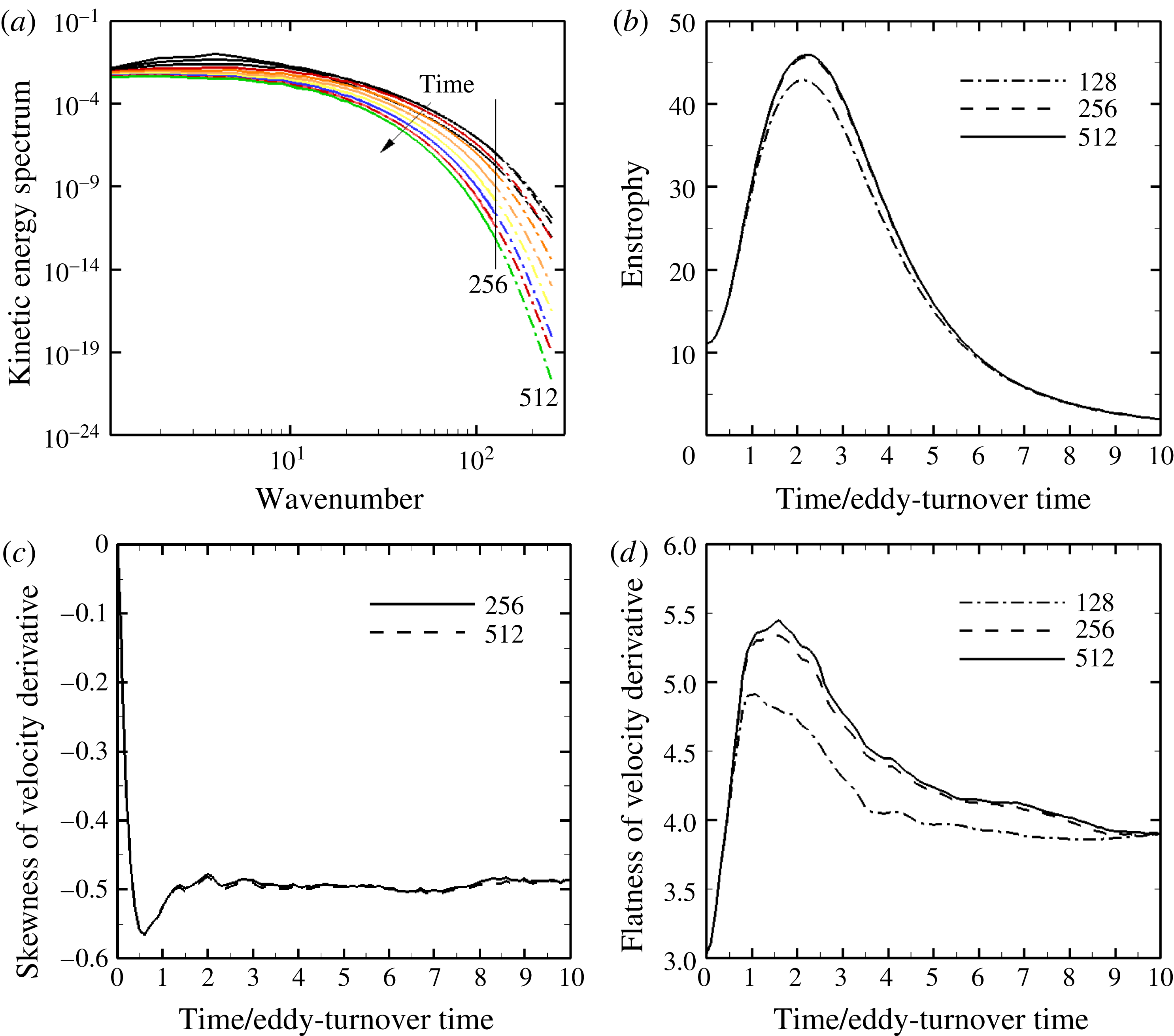
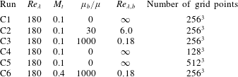
). Table 2 summarizes the flow parameters and grid resolutions of the simulations. Figure 1 demonstrates that a grid of
 $256^{3}$
is sufficiently fine. Considering the C1 and C5 runs, we observe that wavenumbers up to 128 are well resolved on a
 $256^{3}$
grid, which is slightly larger than the reciprocal of the initial Kolmogorov scale
 $\unicode[STIX]{x1D702}$
; the criterion
 $k_{max}\unicode[STIX]{x1D702}\approx 1.5$
is nearly satisfied (Yeung & Pope Reference Yeung and Pope1989). Furthermore, enstrophy, skewness and flatness of velocity derivatives are well resolved, so that we use 256 equidistant points per domain length in each direction.
Summary of the parameters chosen for the simulations.
Convergence study for simulations of the decay of compressible, homogeneous, isotropic turbulence, with zero bulk viscosity: energy spectra for the first ten eddy-turnover times (a; runs C1, C5), and time history of enstrophy (b; runs C1, C4, C5), skewness of the velocity derivative (c; runs C1, C4, C5) and flatness of the velocity derivative (d; runs C1, C4, C5).

3 Results and discussion
3.1 Time evolution of mean flow quantities
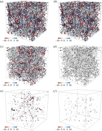
To qualitatively illustrate some of the main effects of bulk viscosity on turbulence, figure 2 shows snapshots of eddies identified by the
 $Q$
-criterion and coloured by dilatation, for
 $\unicode[STIX]{x1D707}_{b}/\unicode[STIX]{x1D707}=0$
and 1000. The two sets of simulations start with the same initial state of turbulence, as described in the previous section. Over time, the density of vortical structures – intended to represent the turbulence – decreases, in both cases. As evidenced by the colouring, the magnitude of the dilatation is greatly reduced for the high bulk viscosity case, while there is little difference in the distribution of eddies; this observation is evident particularly after two eddy-turnover times, where localized regions of high dilatation are observed in the case with zero bulk viscosity, compared to little dilatational variations for
 $\unicode[STIX]{x1D707}_{b}/\unicode[STIX]{x1D707}=1000$
. After
 $5\unicode[STIX]{x1D70F}$
, fewer eddies are visible for the high bulk viscosity case, which is indicative of increased dissipation. At that time, dilatation appears to be uniform and negligible; on the other hand, there is still some variation in dilatation for the case with zero bulk viscosity.
Snapshot of turbulent eddies extracted by the
 $Q$
-criterion and coloured by dilatation at times 0 (a,b), 2 (c,d) and 5 (e,f) for decaying turbulence with
 $\unicode[STIX]{x1D707}_{b}/\unicode[STIX]{x1D707}=0$
(a,c,e) and 1000 (b,d,f).

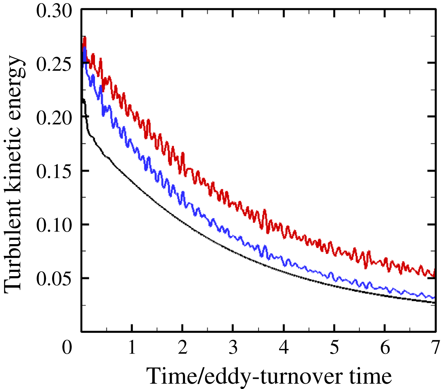
Time evolution of the mean turbulent kinetic energy for
 $\unicode[STIX]{x1D707}_{b}/\unicode[STIX]{x1D707}=0$
(red), 30 (blue) and 1000 (black).

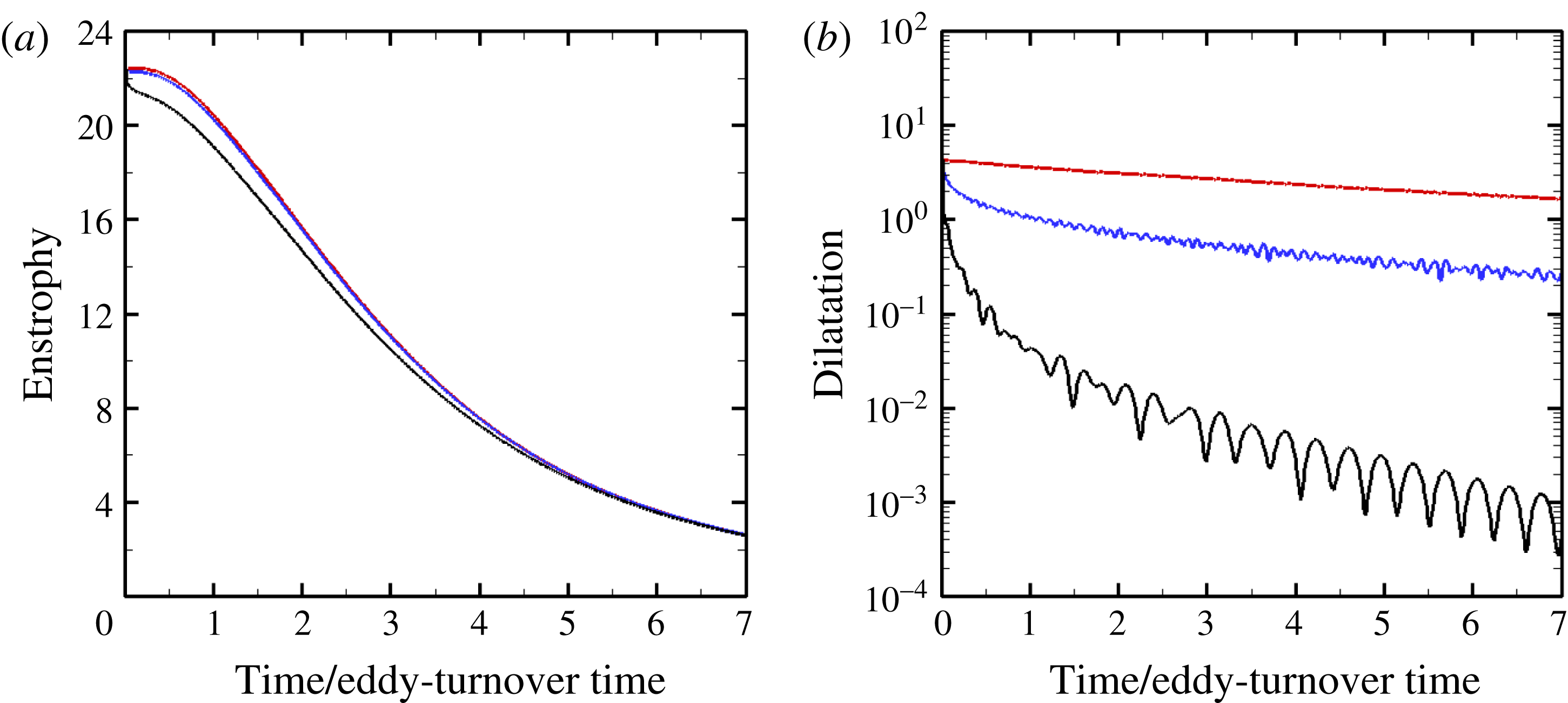
Time evolution of the mean enstrophy (a), and dilatation (b) for
 $\unicode[STIX]{x1D707}_{b}/\unicode[STIX]{x1D707}=0$
(red), 30 (blue) and 1000 (black).

To quantify these observations, we consider the time evolution of the mean turbulent kinetic energy per unit volume (TKE),
 $K=\langle \unicode[STIX]{x1D70C}u_{i}u_{i}/2\rangle$
, where the brackets denote spatial averages, in figure 3, as well as enstrophy and dilatation in figure 4. The TKE decreases with time in a mostly uniform fashion with small fluctuations due to the initially generated acoustic waves, consistent with the observations of Miura & Kida (Reference Miura and Kida1995). Bulk viscosity enhances the turbulent kinetic energy dissipation, especially early on for large
 $\unicode[STIX]{x1D707}_{b}$
; it takes approximately a tenth of an eddy-turnover time for the flow to adjust to the introduction of bulk viscosity. After approximately
 $2\unicode[STIX]{x1D70F}$
, the decay rates are comparable in all three cases, thus suggesting that the main action of bulk viscosity occur within the first couple of eddy-turnover times. Another outcome of increasing bulk viscosity is the damping of the unsteadiness due to increased compressive dissipation (discussed in § 3.3). Enstrophy decreases with time, although the relative reduction due to bulk viscosity is not as significant as for the TKE; the
 $\unicode[STIX]{x1D707}_{b}/\unicode[STIX]{x1D707}=0$
and 30 cases are almost indistinguishable on this scale. The more dramatic effects of bulk viscosity pertain to compressibility. For
 $\unicode[STIX]{x1D707}_{b}/\unicode[STIX]{x1D707}=1000$
, the dilatation decreases rapidly with increasing bulk viscosity, by two orders of magnitude in the first two eddy-turnover times. On this logarithmic scale, constant-period oscillations are evident after approximately
 $4\unicode[STIX]{x1D70F}$
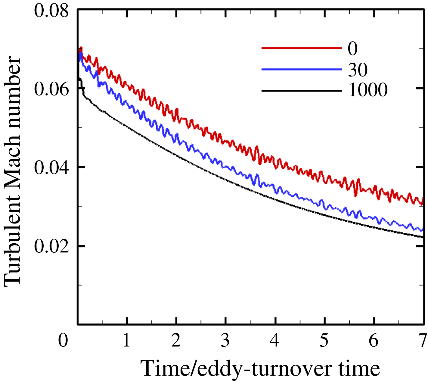
. Since the initial conditions are not in acoustic equilibrium, acoustic waves are produced at the beginning of the simulation. Viscous dissipation damps these waves from highest wavenumbers to lowest, such that the oscillations observed in the dilatation are manifestations of the fundamental frequency of the box. Over the course of the simulation, the turbulent Mach number steadily decreases (figure 5), following the same behaviour as the TKE since both depend on
 $u_{rms}$
and the mean sound speed does not change substantially. These observations suggest that after approximately two eddy-turnover times the dominant modes are vortical, rather than acoustic or entropic (Kovasznay Reference Kovasznay1988; Gatski & Bonnet Reference Gatski and Bonnet2013) for
 $\unicode[STIX]{x1D707}_{b}/\unicode[STIX]{x1D707}=1000$
. We show later that these compressibility results are due to the damping of dilatational modes by bulk viscosity.
Time evolution of the turbulent Mach number for
 $\unicode[STIX]{x1D707}_{b}/\unicode[STIX]{x1D707}=0$
(red), 30 (blue) and 1000 (black).

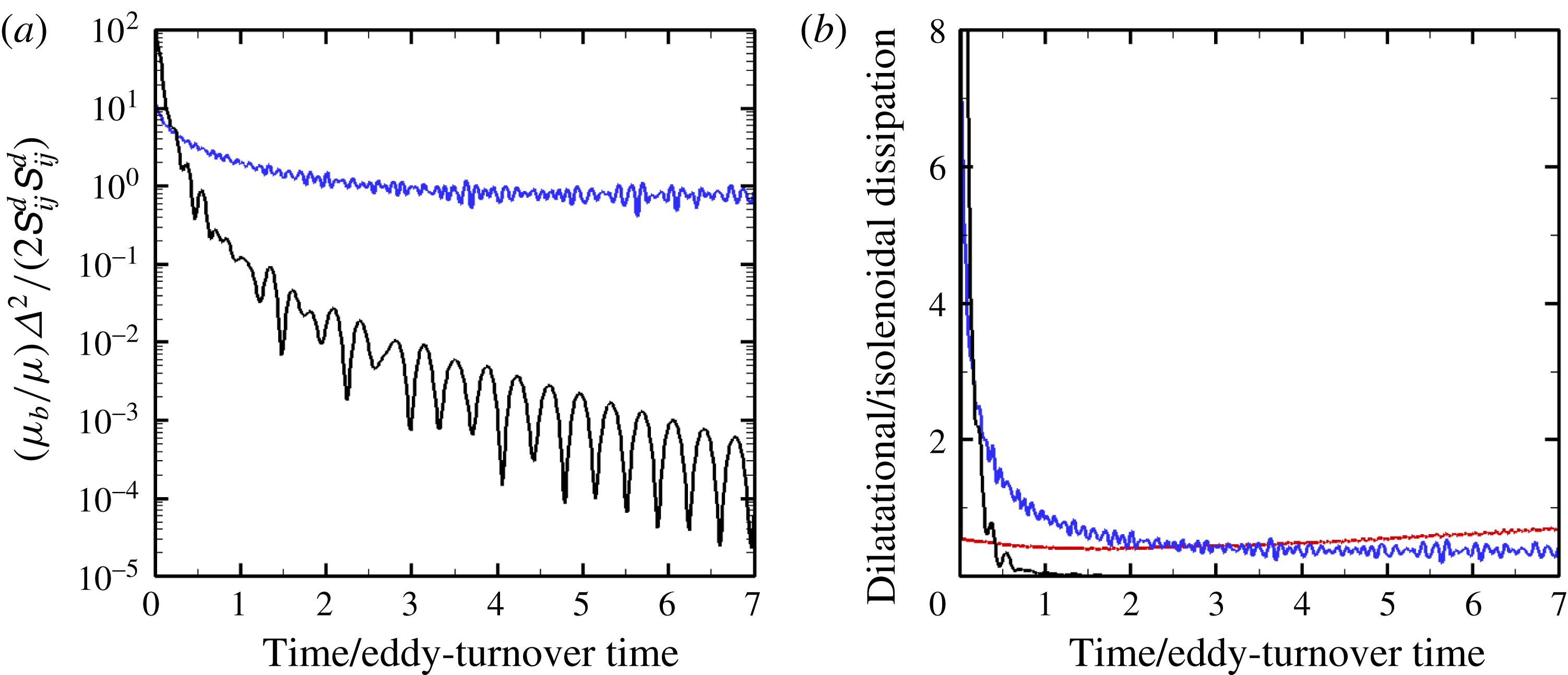
The above observations can be qualitatively understood by considering the ratios of bulk to shear viscous dissipation
 $\unicode[STIX]{x1D6F7}$
and the dilatational to solenoidal dissipation
 $\unicode[STIX]{x1D6F9}$
:
 $$\begin{eqnarray}\unicode[STIX]{x1D6F7}=\frac{\unicode[STIX]{x1D707}_{b}}{\unicode[STIX]{x1D707}}\frac{\langle \unicode[STIX]{x1D6E5}^{2}\rangle }{{\textstyle \frac{4}{3}}\langle \unicode[STIX]{x1D6E5}^{2}\rangle +\langle \unicode[STIX]{x1D714}_{k}\unicode[STIX]{x1D714}_{k}\rangle },\quad \unicode[STIX]{x1D6F9}=\frac{\displaystyle \left(\frac{4}{3}+\frac{\unicode[STIX]{x1D707}_{b}}{\unicode[STIX]{x1D707}}\right)\langle \unicode[STIX]{x1D6E5}^{2}\rangle }{\langle \unicode[STIX]{x1D714}_{k}\unicode[STIX]{x1D714}_{k}\rangle },\end{eqnarray}$$
where
 $\unicode[STIX]{x1D714}_{k}$
is the vorticity. Figure 6 shows the time evolution of these two quantities. The relative importance of bulk vs. shear viscous dissipation strongly depends on bulk viscosity. Although bulk viscous dissipation starts nearly a hundred times larger than the shear viscous dissipation for the
 $\unicode[STIX]{x1D707}_{b}/\unicode[STIX]{x1D707}=1000$
case,
 $\unicode[STIX]{x1D6F7}$
becomes less than one within
 $0.5\unicode[STIX]{x1D70F}$
, beyond which time the bulk viscous dissipation is negligible. As
 $\unicode[STIX]{x1D707}_{b}/\unicode[STIX]{x1D707}$
is reduced,
 $\unicode[STIX]{x1D6F7}$
decreases more slowly; at late times, the contribution of bulk viscous dissipation remains nearly constant, within 10 %–20 % of the shear viscous dissipation, such that bulk viscous effects are not negligible.
Time evolution of the bulk to shear viscous dissipation
 $\unicode[STIX]{x1D6F7}$
(a) and dilatational to solenoidal dissipation
 $\unicode[STIX]{x1D6F9}$
(b) for
 $\unicode[STIX]{x1D707}_{b}/\unicode[STIX]{x1D707}=0$
(red; b only), 30 (blue) and 1000 (black).

A knowledge of the origin of dissipation is important when modelling compressible turbulence (Lele Reference Lele1994). The relative importance of dilatational vs. solenoidal dissipation also strongly depends on bulk viscosity. When there is no bulk viscosity, the ratio between dilatational and solenoidal dissipation lies between 0.4 and 0.7 throughout the simulation, thus highlighting the larger solenoidal contribution. For
 $\unicode[STIX]{x1D707}_{b}/\unicode[STIX]{x1D707}=30$
, the initial compressive dissipation rate is several times larger than the solenoidal dissipation; it subsequently decreases to reach a mean value of approximately 0.3 within
 $4\unicode[STIX]{x1D70F}$
, which is not entirely negligible. For the highest bulk viscosity, the compressive dissipation rate is even larger initially, but then decreases to nearly zero within an eddy-turnover time as a result of the damping of the dilatational modes for
 $\unicode[STIX]{x1D707}_{b}/\unicode[STIX]{x1D707}=1000$
. Over time, the dilatational contribution thus continuously decreases to become nearly negligible at a finite time.
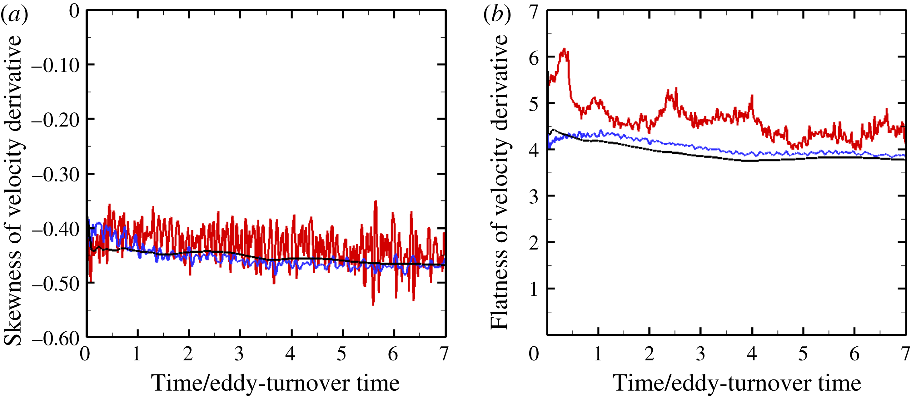
The time evolutions of the skewness and flatness of the velocity derivatives,
 $$\begin{eqnarray}\displaystyle & \displaystyle \text{Skewness}=\frac{1}{3}\left(\frac{\displaystyle \left\langle \left(\frac{\unicode[STIX]{x2202}u_{1}}{\unicode[STIX]{x2202}x_{1}}\right)^{3}\right\rangle }{\displaystyle \left\langle \left(\frac{\unicode[STIX]{x2202}u_{1}}{\unicode[STIX]{x2202}x_{1}}\right)^{2}\right\rangle ^{3/2}}+\frac{\displaystyle \left\langle \left(\frac{\unicode[STIX]{x2202}u_{2}}{\unicode[STIX]{x2202}x_{2}}\right)^{3}\right\rangle }{\displaystyle \left\langle \left(\frac{\unicode[STIX]{x2202}u_{2}}{\unicode[STIX]{x2202}x_{2}}\right)^{2}\right\rangle ^{3/2}}+\frac{\displaystyle \left\langle \left(\frac{\unicode[STIX]{x2202}u_{3}}{\unicode[STIX]{x2202}x_{3}}\right)^{3}\right\rangle }{\displaystyle \left\langle \left(\frac{\unicode[STIX]{x2202}u_{3}}{\unicode[STIX]{x2202}x_{3}}\right)^{2}\right\rangle ^{3/2}}\right), & \displaystyle\end{eqnarray}$$
 $$\begin{eqnarray}\displaystyle & \displaystyle \text{Flatness}=\frac{1}{3}\left(\frac{\displaystyle \left\langle \left(\frac{\unicode[STIX]{x2202}u_{1}}{\unicode[STIX]{x2202}x_{1}}\right)^{4}\right\rangle }{\displaystyle \left\langle \left(\frac{\unicode[STIX]{x2202}u_{1}}{\unicode[STIX]{x2202}x_{1}}\right)^{2}\right\rangle ^{2}}+\frac{\displaystyle \left\langle \left(\frac{\unicode[STIX]{x2202}u_{2}}{\unicode[STIX]{x2202}x_{2}}\right)^{4}\right\rangle }{\displaystyle \left\langle \left(\frac{\unicode[STIX]{x2202}u_{2}}{\unicode[STIX]{x2202}x_{2}}\right)^{2}\right\rangle ^{2}}+\frac{\displaystyle \left\langle \left(\frac{\unicode[STIX]{x2202}u_{3}}{\unicode[STIX]{x2202}x_{3}}\right)^{4}\right\rangle }{\displaystyle \left\langle \left(\frac{\unicode[STIX]{x2202}u_{3}}{\unicode[STIX]{x2202}x_{3}}\right)^{2}\right\rangle ^{2}}\right), & \displaystyle\end{eqnarray}$$
are shown in figure 7. The introduction of bulk viscosity has a stabilizing effect associated with smaller fluctuations in these quantities. The higher the bulk viscosity, the sooner the equilibrium expected for incompressible turbulence is reached (close to
 $-0.45$
for skewness and
 $4.0$
for flatness, Pope Reference Pope2000).
Time evolution of the skewness (a) and flatness (b) of the velocity derivatives for
 $\unicode[STIX]{x1D707}_{b}/\unicode[STIX]{x1D707}=0$
(red), 30 (blue) and 1000 (black).

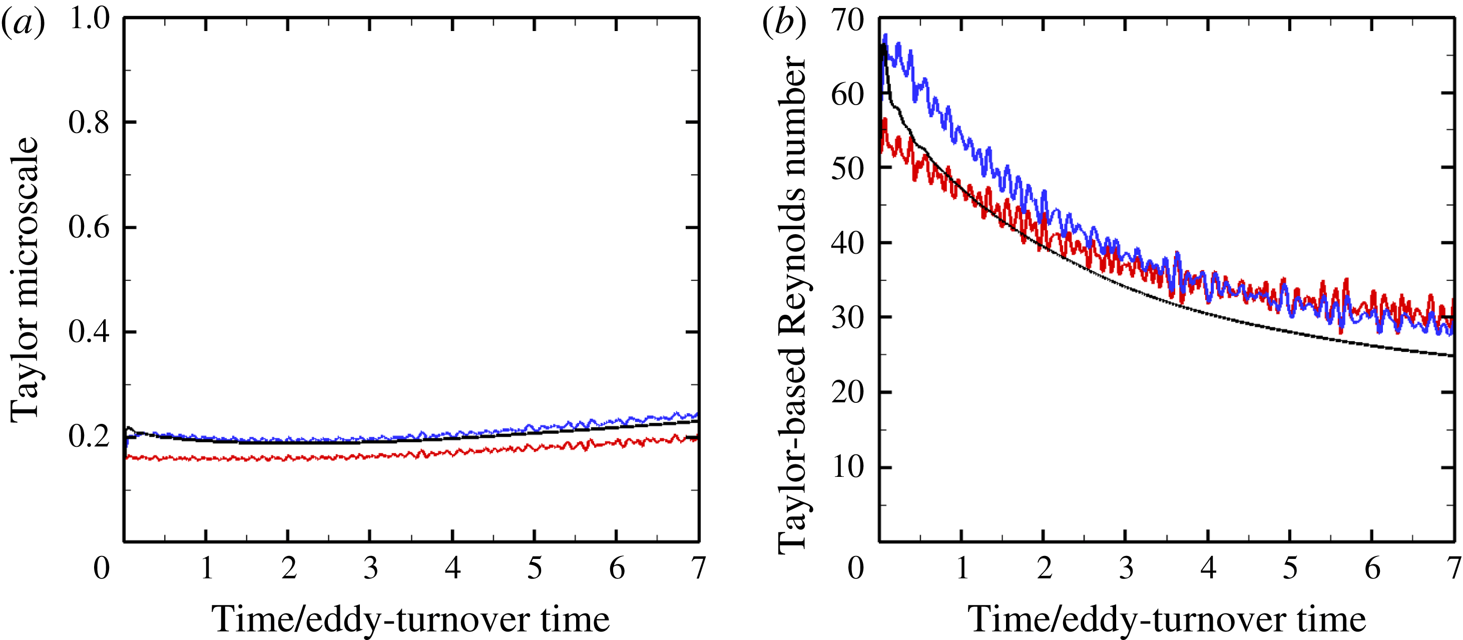
The time evolutions of the Taylor microscale and Taylor-based Reynolds number,
 $$\begin{eqnarray}\unicode[STIX]{x1D706}=\sqrt{\frac{\left\langle u_{1}^{2}\right\rangle +\left\langle u_{2}^{2}\right\rangle +\left\langle u_{3}^{2}\right\rangle }{\displaystyle \left\langle \left(\frac{\unicode[STIX]{x2202}u_{1}}{\unicode[STIX]{x2202}x_{1}}\right)^{2}\right\rangle +\left\langle \left(\frac{\unicode[STIX]{x2202}u_{2}}{\unicode[STIX]{x2202}x_{2}}\right)^{2}\right\rangle +\left\langle \left(\frac{\unicode[STIX]{x2202}u_{3}}{\unicode[STIX]{x2202}x_{3}}\right)^{2}\right\rangle }},\quad Re_{\unicode[STIX]{x1D706}}=\frac{\left\langle \unicode[STIX]{x1D70C}\right\rangle u_{rms}\unicode[STIX]{x1D706}}{\unicode[STIX]{x1D707}},\end{eqnarray}$$
are shown in figure 8. Over the course of the simulations, the Taylor scale does not change significantly. In the absence of bulk viscosity,
 $\unicode[STIX]{x1D706}$
exhibits nearly no growth for
 $2{-}3\unicode[STIX]{x1D70F}$
before slightly increasing. In the presence of bulk viscosity, the Taylor scale exhibits a rapid initial increase (by nearly 30 % within
 $0.1\unicode[STIX]{x1D70F}$
) due to dilatational dissipation (discussed in the next section). As the flow adjusts to this new state of turbulence, the Taylor scale decreases over
 $1{-}2\unicode[STIX]{x1D70F}$
before gradually increasing. Given the consistent decrease in turbulent kinetic energy (figure 3), this increase is due to a decrease in the magnitude of the fluctuating strain field as the turbulence adjusts to the new conditions prescribed by bulk viscosity. Although the growth over time depends on
 $\unicode[STIX]{x1D707}_{b}$
, the rate is similar for the different bulk viscosities after approximately
 $4\unicode[STIX]{x1D70F}$
. Interestingly, the case
 $\unicode[STIX]{x1D707}_{b}/\unicode[STIX]{x1D707}=30$
has the largest Taylor scale over the time interval under consideration, due to the weaker decrease (compared to the high
 $\unicode[STIX]{x1D707}_{b}$
case) following the introduction of bulk viscosity. The behaviour of
 $Re_{\unicode[STIX]{x1D706}}$
combines the trends observed in
 $u_{rms}$
(figure 5) and
 $\unicode[STIX]{x1D706}$
. In the absence of bulk viscosity,
 $Re_{\unicode[STIX]{x1D706}}$
continuously decreases. The introduction of bulk viscosity gives rise to an initial increase in the Reynolds number, just like for the Taylor scale, although it is mitigated by the initial decrease in
 $u_{rms}$
. Thereafter, the decrease in
 $Re_{\unicode[STIX]{x1D706}}$
for the cases with bulk viscosity is dominated by the decrease in intensity, rather than the increasing Taylor scale, with similar slopes for the
 $\unicode[STIX]{x1D707}_{b}/\unicode[STIX]{x1D707}=30$
and 1000 cases. On the other hand, the rate at which
 $Re_{\unicode[STIX]{x1D706}}$
decreases is lower in the absence of bulk viscosity, a trend consistent with the behaviour of
 $u_{rms}$
.
Time evolution of mean flow quantities for
 $\unicode[STIX]{x1D707}_{b}/\unicode[STIX]{x1D707}=0$
(red), 30 (blue) and 1000 (black). (a) Taylor microscale; (b) Taylor-based Reynolds number.

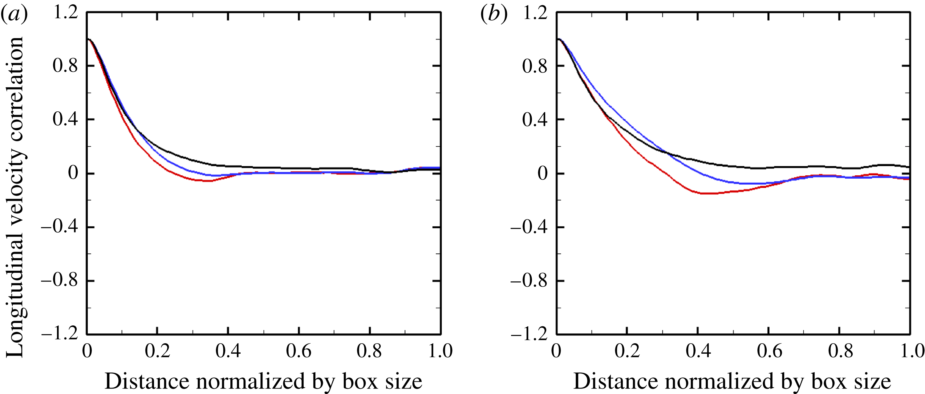
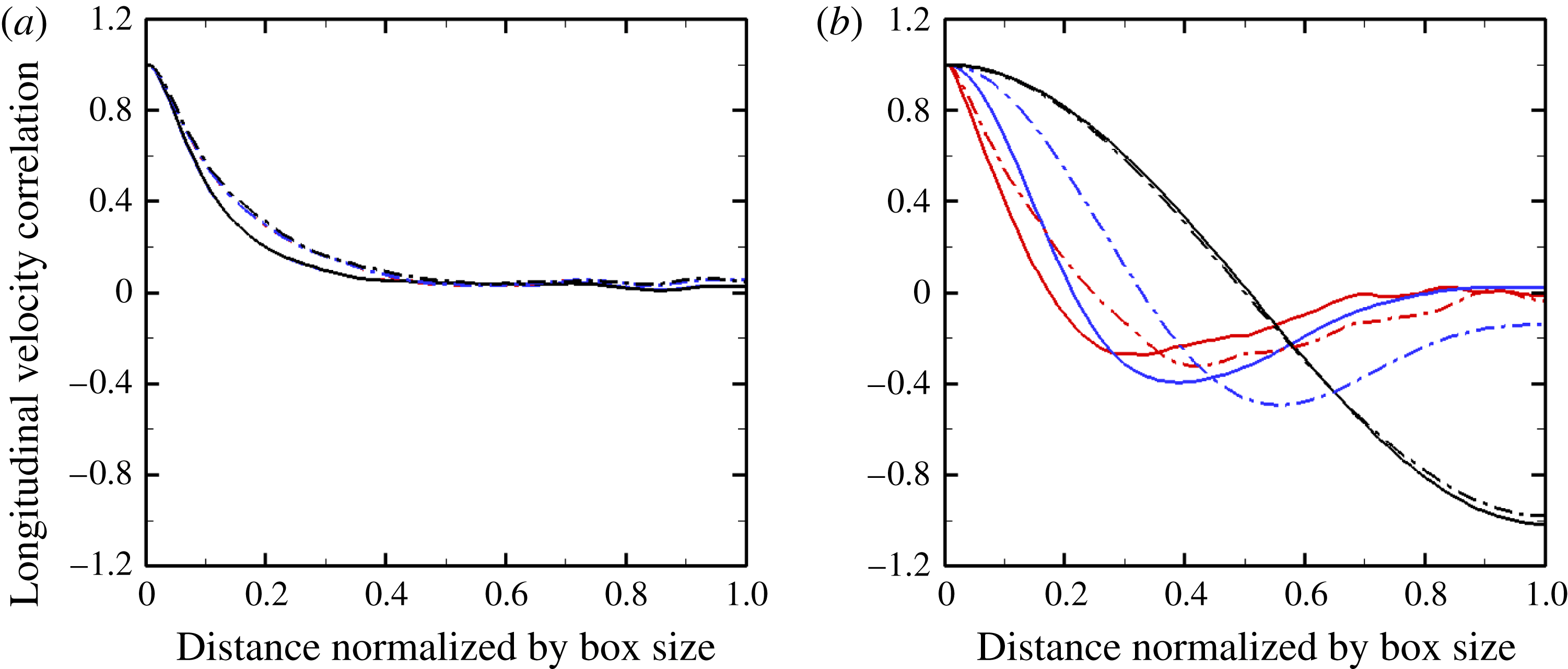
Figure 9 shows the longitudinal velocity correlation,
 $\langle u_{i}(x+r)u_{i}(x)\rangle /\langle u_{i}^{2}(x)\rangle$
(no sum implied) at
 $2\unicode[STIX]{x1D70F}$
and
 $7\unicode[STIX]{x1D70F}$
, with the
 $x$
-axis normalized by half the domain size. The simulations with bulk viscosity exhibit small differences from that with zero bulk viscosity starting from
 $x=0$
. At
 $2\unicode[STIX]{x1D70F}$
, the
 $\unicode[STIX]{x1D707}_{b}/\unicode[STIX]{x1D707}=1000$
case starts to diverge from the
 $\unicode[STIX]{x1D707}_{b}/\unicode[STIX]{x1D707}=30$
curve at a distance of approximately 0.15, thus illustrating the fact that bulk viscosity enhances the spatial correlation and implying that the range of influence of the turbulence is increased. The
 $\unicode[STIX]{x1D707}_{b}/\unicode[STIX]{x1D707}=0$
and 30 cases exhibit a minimum (negative correlation), which shifts farther in space with time. This non-intuitive behaviour of the correlation is due to the combination of solenoidal and dilatational velocity components, as explained in greater detail in the next section.
3.2 Helmholtz decomposed fields
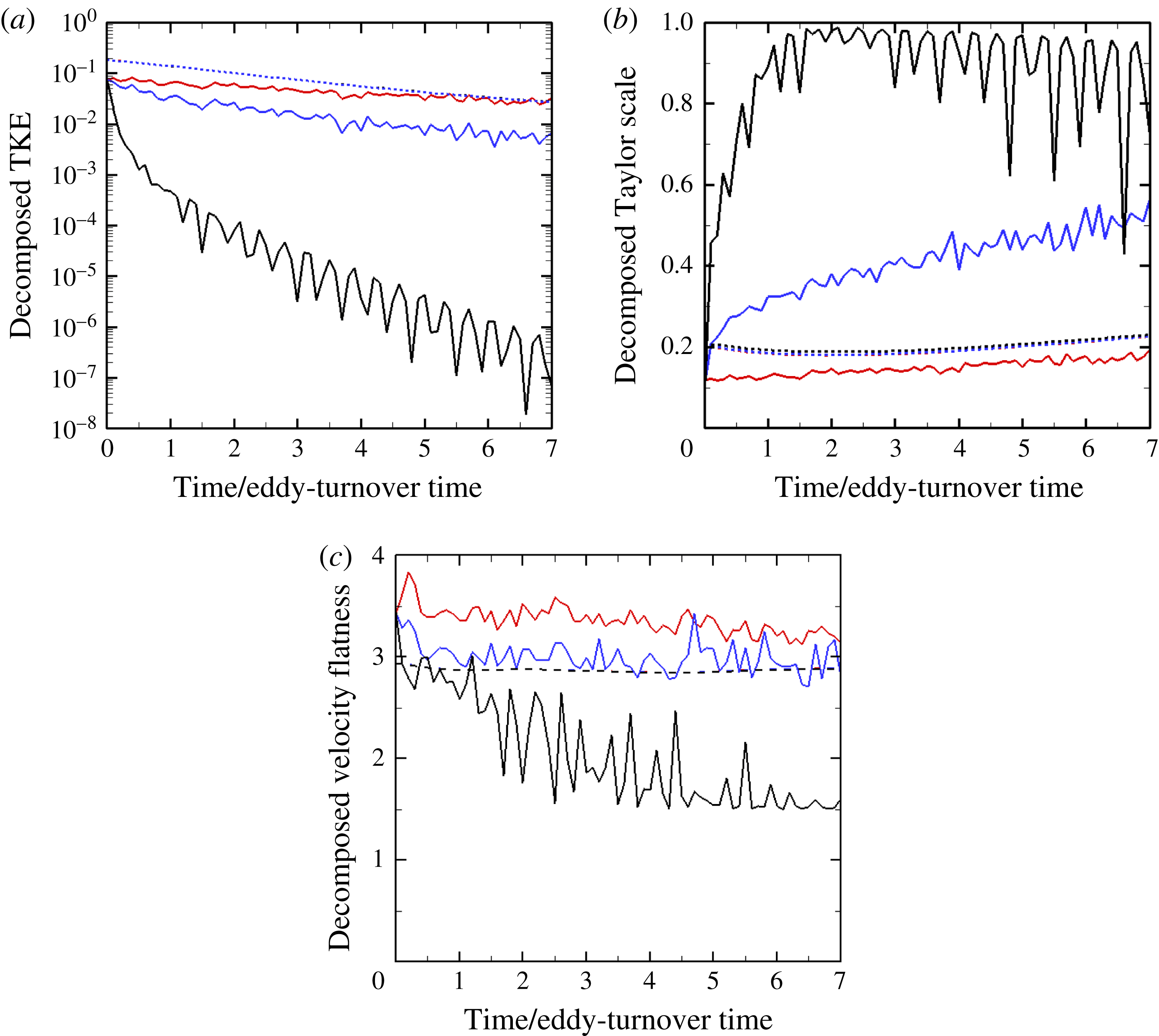
The starkly different dependence of enstrophy and dilatation on bulk viscosity suggests decomposing the flow into solenoidal and dilatational velocity components to shed light into the dynamics and energetics. Figure 10 shows the time evolution of the TKE, Taylor scale and flatness of the decomposed velocity. The TKE corresponding to the solenoidal velocity shows little dependence on the bulk viscosity (the curves are almost indistinguishable in the figure). However, that corresponding to the dilatational velocity exhibits a faster decay, particularly for the
 $\unicode[STIX]{x1D707}_{b}/\unicode[STIX]{x1D707}=1000$
case – by six decades over the seven eddy-turnover times. If there is no bulk viscosity, the dilatational TKE decays at a slower rate than the solenoidal component due to lower dissipation. This observation is consistent with the low bulk-viscosity-based Reynolds numbers in table 2: the dilatational field is expected to experience high bulk viscous dissipation at early times and to rapidly decay thereafter (discussed in the next section). Similarly, a much larger Taylor scale corresponding to the dilatational velocity is achieved, saturating within one eddy-turnover time as it reaches the box size; this observation also explains the larger longitudinal velocity correlation in figure 9. The Taylor scale corresponding to the solenoidal velocity follows the trends in figure 8(a), in which the non-monotonic behaviour with respect to
 $\unicode[STIX]{x1D707}_{b}$
is attributed to the competition between the dilatational and solenoidal modes. The flatness of the velocity corresponding to the solenoidal velocity exhibits nearly no dependence on bulk viscosity and reaches a value of three expected for incompressible turbulence. On the other hand, for the dilatational velocity, the flatness of the dilatational velocity is mostly larger than three for the
 $\unicode[STIX]{x1D707}_{b}/\unicode[STIX]{x1D707}=0$
and 30 cases. For the high bulk viscosity case, the flatness oscillates about a much lower mean value (approximately 1.5). These results further suggest that the solenoidal and dilatational components decouple, with the latter exhibiting a strong dependence on bulk viscosity.
Longitudinal velocity correlation at
 $2\unicode[STIX]{x1D70F}$
(a) and
 $7\unicode[STIX]{x1D70F}$
(b) for
 $\unicode[STIX]{x1D707}_{b}/\unicode[STIX]{x1D707}=0$
(red), 30 (blue) and 1000 (black).

Time evolution of turbulent kinetic energy (a), Taylor microscale (b) and flatness of the velocity derivatives (c) for
 $\unicode[STIX]{x1D707}_{b}/\unicode[STIX]{x1D707}=0$
(red), 30 (blue) and 1000 (black), in which the velocity has been decomposed into solenoidal (dotted) and dilatational (solid) components. Note that the curves corresponding to the solenoidal component are nearly indistinguishable at this scale.

The behaviour observed in the velocity correlations of figure 9 are readily explained by considering the decomposed fields. Figure 11 shows the decomposed velocity correlations at
 $2\unicode[STIX]{x1D70F}$
and
 $7\unicode[STIX]{x1D70F}$
. The correlation exhibits little dependence on the bulk viscosity for the solenoidal component: the correlation is amplified by 10–30 % for distances between 0.1 and 0.4. More substantial amplification is observed for the dilatational component, except for the largest
 $\unicode[STIX]{x1D707}_{b}/\unicode[STIX]{x1D707}$
case. When no bulk viscosity is present, the correlation decreases to negative values, with a minimum of approximately 0.25 after
 $2\unicode[STIX]{x1D70F}$
; the correlation then increases back to zero. At a later time, the minimum shifts farther and decreases. A qualitatively similar behaviour is observed for
 $\unicode[STIX]{x1D707}_{b}/\unicode[STIX]{x1D707}=30$
. For the largest bulk viscosity, the correlation smoothly decreases from 1.0 to
 $-1.0$
, thus indicating the presence of a standing wave whose wavelength is half the box size. This observation indicates that the acoustic waves produced by the initial conditions persist, consistent with previous studies (Kida & Orszag Reference Kida and Orszag1992).
Longitudinal velocity correlation at
 $2\unicode[STIX]{x1D70F}$
(solid) and
 $7\unicode[STIX]{x1D70F}$
(dash-dotted) for the solenoidal (a) and dilatational (b) velocity components, for
 $\unicode[STIX]{x1D707}_{b}/\unicode[STIX]{x1D707}=0$
(red), 30 (blue) and 1000 (black).

3.3 Budgets
3.3.1 Kinetic energy transport
For conciseness, only the cases with
 $\unicode[STIX]{x1D707}_{b}/\unicode[STIX]{x1D707}=0$
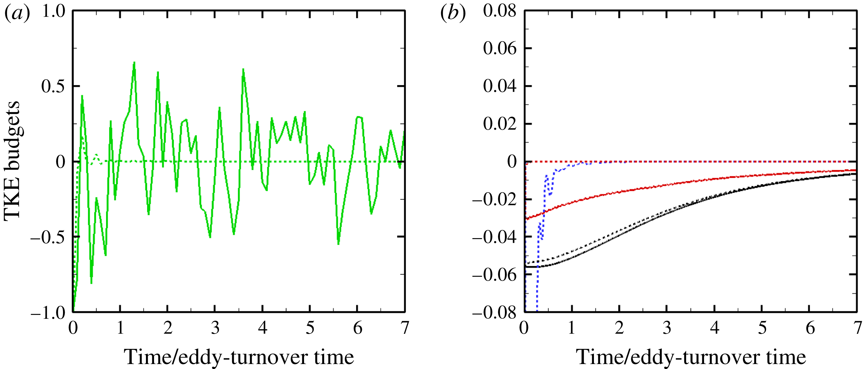
and 1000 are considered until the end of § 3.4. For compressible, homogeneous, isotropic turbulence, the transport equation for turbulent kinetic energy
 $K=\unicode[STIX]{x1D70C}u_{i}u_{i}/2$
can be written:
 $$\begin{eqnarray}\frac{\text{d}\langle K\rangle }{\text{d}t}=\langle p\unicode[STIX]{x0394}\rangle -\frac{1}{Re}\left(\langle \unicode[STIX]{x1D74E}\boldsymbol{\cdot }\unicode[STIX]{x1D74E}\rangle +\frac{4}{3}\langle \unicode[STIX]{x1D6E5}^{2}\rangle +\frac{\unicode[STIX]{x1D707}_{b}}{\unicode[STIX]{x1D707}}\langle \unicode[STIX]{x1D6E5}^{2}\rangle \right),\end{eqnarray}$$
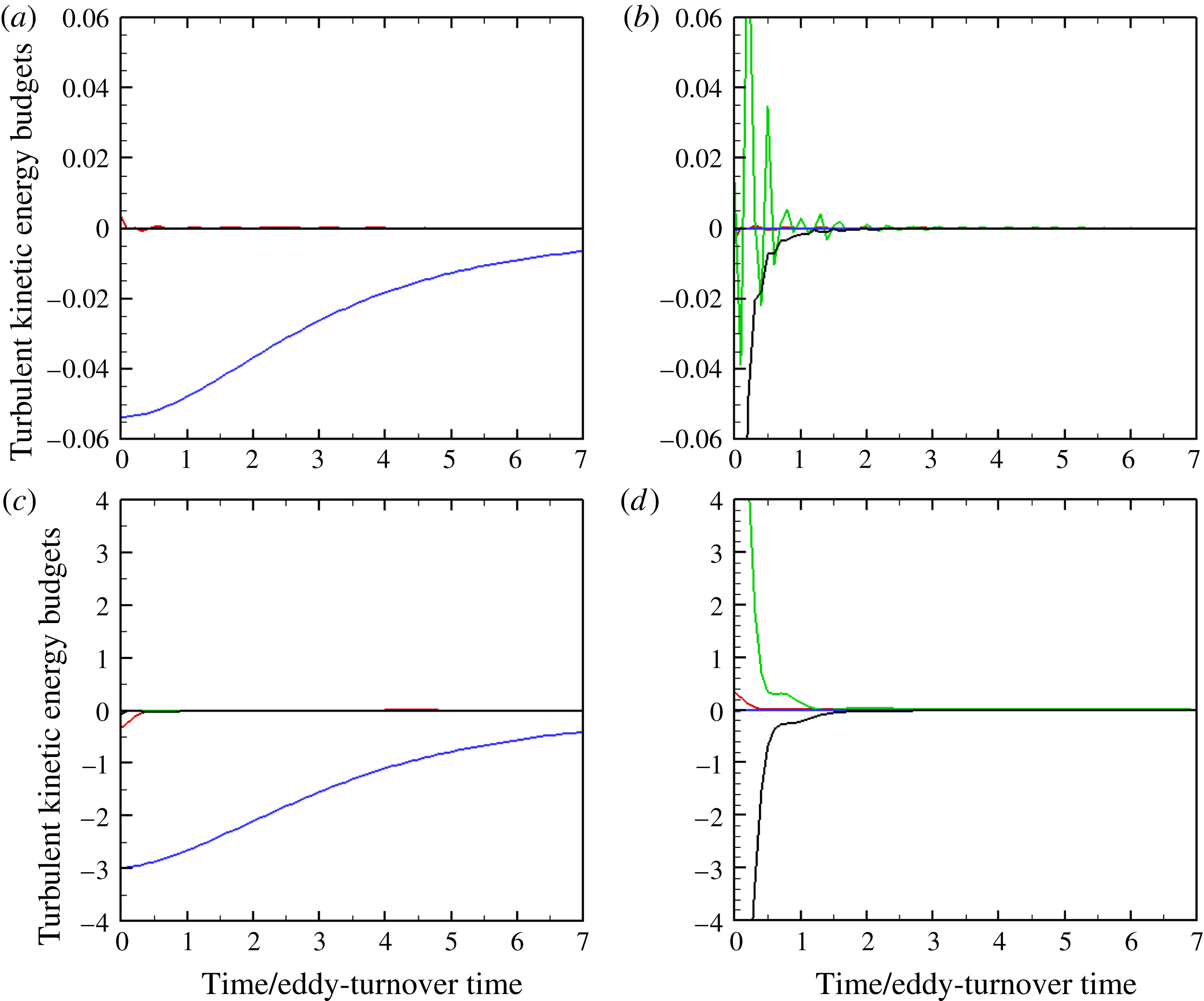
where the terms on the right-hand side are pressure–dilatation, solenoidal dissipation, compressible dissipation due to shear viscosity and compressible dissipation due to bulk viscosity; these terms are shown in figure 12, with pressure–dilatation plotted separately because its magnitude is far greater than the other terms.
Time evolution of the turbulent kinetic energy budgets for
 $\unicode[STIX]{x1D707}_{b}/\unicode[STIX]{x1D707}=0$
(solid) and 1000 (dotted). (a) Pressure–dilatation term only; (b) terms in brackets in equation (black: solenoidal dissipation; red: shear dilatational dissipation; blue: bulk dilatational dissipation).

The reversible work done by thermodynamic pressure corresponds to exchange between internal and kinetic energy. With no bulk viscosity, this quantity oscillates about zero, progressively decreasing in magnitude. In the presence of bulk viscosity, this term is reduced by 95 % within
 $0.5\unicode[STIX]{x1D70F}$
due to the considerable reduction in dilatation but remains substantial when
 $\unicode[STIX]{x1D707}_{b}=0$
. Thus, exchanges between internal and kinetic energy are prevented when
 $\unicode[STIX]{x1D707}_{b}$
is large.
Shear solenoidal dissipation starts at the same level for both values of bulk viscosity, as does dilatational dissipation. When there is no bulk viscosity, both decrease over time as the turbulence intensity decreases, with the compressible contribution approximately half that of the solenoidal. In the presence of bulk viscosity, the main dissipative contribution comes from bulk dilatational dissipation, which starts at a value of
 $-20$
(off the plot) and decreases to a negligible contribution within the first eddy-turnover time. The shear dilatational dissipation becomes negligible within
 $0.1\unicode[STIX]{x1D70F}$
; the shear solenoidal dissipation initially decreases slightly before following a behaviour close to that of the
 $\unicode[STIX]{x1D707}_{b}=0$
case. For
 $\unicode[STIX]{x1D707}_{b}/\unicode[STIX]{x1D707}=1000$
, TKE dissipation rapidly becomes dominated by solenoidal dissipation owing to the negligible contribution of the dissipative terms involving dilatation in (3.5). These results explain the substantial decrease of the decomposed TKE in figure 10.
Following Kida & Orszag (Reference Kida and Orszag1992), Helmholtz decomposition is used to develop time evolution equations for solenoidal and dilatational TKE contributions. From the continuity and momentum balance equations, the time evolution of
 $w_{i}$
, defined in (2.5), can be written:
 $$\begin{eqnarray}\frac{\unicode[STIX]{x2202}w_{i}}{\unicode[STIX]{x2202}t}=-u_{j}\frac{\unicode[STIX]{x2202}w_{i}}{\unicode[STIX]{x2202}x_{j}}-\frac{1}{2}w_{i}\unicode[STIX]{x0394}-\frac{1}{\sqrt{\unicode[STIX]{x1D70C}}}\frac{\unicode[STIX]{x2202}p}{\unicode[STIX]{x2202}x_{i}}+\frac{2}{Re\sqrt{\unicode[STIX]{x1D70C}}}\frac{\unicode[STIX]{x2202}}{\unicode[STIX]{x2202}x_{j}}\left(\unicode[STIX]{x1D61A}_{ij}-\frac{1}{3}\unicode[STIX]{x0394}\unicode[STIX]{x1D6FF}_{ij}\right)+\frac{1}{Re\sqrt{\unicode[STIX]{x1D70C}}}\frac{\unicode[STIX]{x1D707}_{b}}{\unicode[STIX]{x1D707}}\frac{\unicode[STIX]{x2202}}{\unicode[STIX]{x2202}x_{j}}(\unicode[STIX]{x0394}\unicode[STIX]{x1D6FF}_{ij}).\end{eqnarray}$$
A spatial average of the inner product of this equation with
 $w_{i}^{(s,d)}$
, where the
 $s$
and
 $d$
superscripts correspond to solenoidal and dilatational, respectively, yields the following time evolution equations for the solenoidal (
 $K^{(s)}=\unicode[STIX]{x1D70C}u_{i}^{(s)}u_{i}^{(s)}/2$
) and dilatational (
 $K^{(d)}=\unicode[STIX]{x1D70C}u_{i}^{(d)}u_{i}^{(d)}/2$
) TKE contributions:
 $$\begin{eqnarray}\displaystyle \frac{\text{d}\langle K^{(s,d)}\rangle }{\text{d}t} & = & \displaystyle \left\langle w_{i}^{(s,d)}\left(-u_{j}\frac{\unicode[STIX]{x2202}w_{i}}{\unicode[STIX]{x2202}x_{j}}-w_{i}\frac{\unicode[STIX]{x1D6E5}}{2}\right)\right\rangle -\left\langle \frac{w_{i}^{(s,d)}}{\sqrt{\unicode[STIX]{x1D70C}}}\frac{\unicode[STIX]{x2202}p}{\unicode[STIX]{x2202}x_{i}}\right\rangle \nonumber\\ \displaystyle & & \displaystyle +\,\frac{2}{Re}\left\langle \frac{w_{i}^{(s,d)}}{\sqrt{\unicode[STIX]{x1D70C}}}\frac{\unicode[STIX]{x2202}}{\unicode[STIX]{x2202}x_{j}}\left(\unicode[STIX]{x1D61A}_{ij}-\frac{\unicode[STIX]{x1D6E5}}{3}\unicode[STIX]{x1D6FF}_{ij}\right)\right\rangle +\frac{1}{Re}\left\langle \frac{w_{i}^{(s,d)}}{\sqrt{\unicode[STIX]{x1D70C}}}\frac{\unicode[STIX]{x1D707}_{b}}{\unicode[STIX]{x1D707}}\frac{\unicode[STIX]{x2202}}{\unicode[STIX]{x2202}x_{j}}(\unicode[STIX]{x0394}\unicode[STIX]{x1D6FF}_{ij})\right\rangle .\end{eqnarray}$$
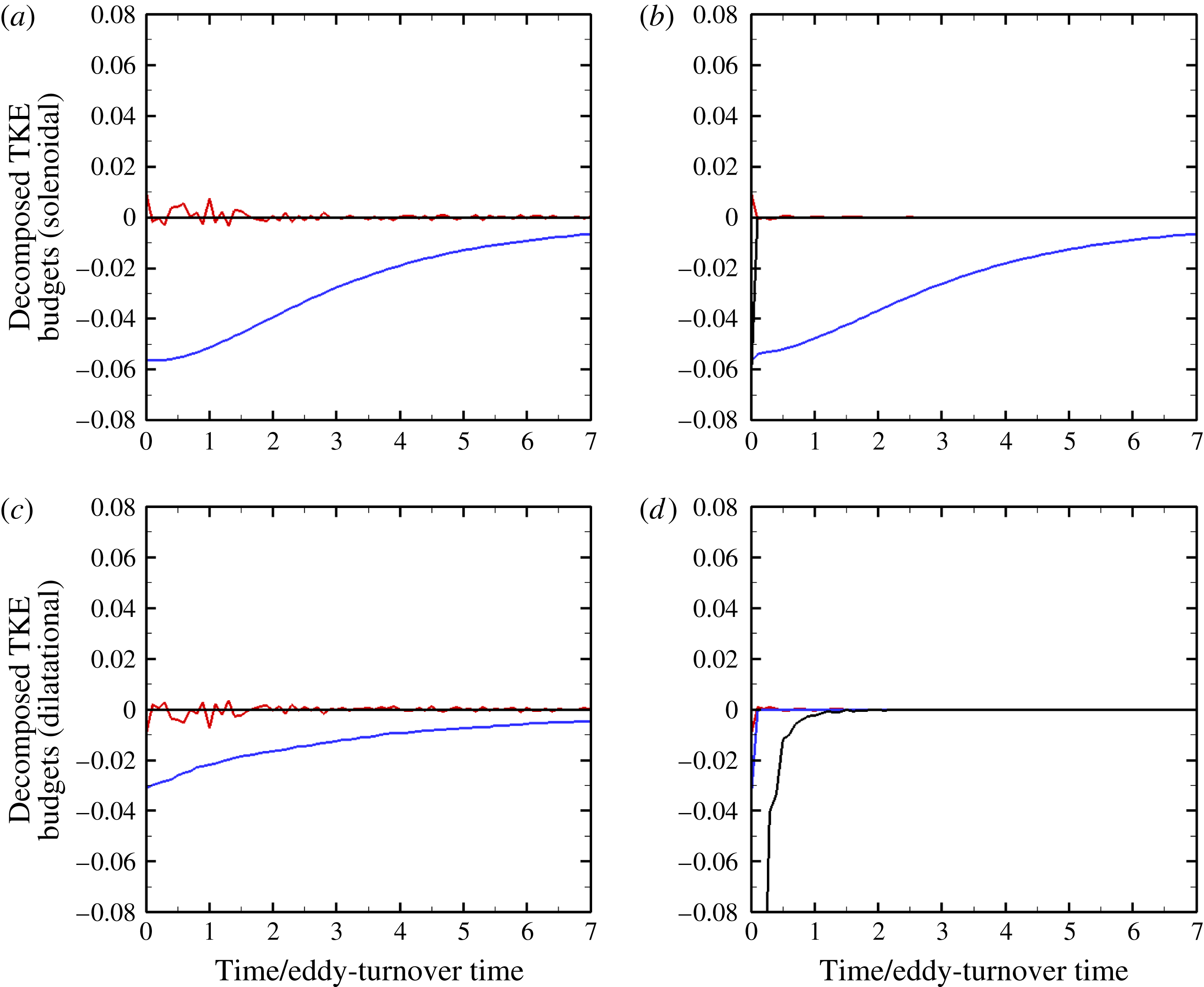
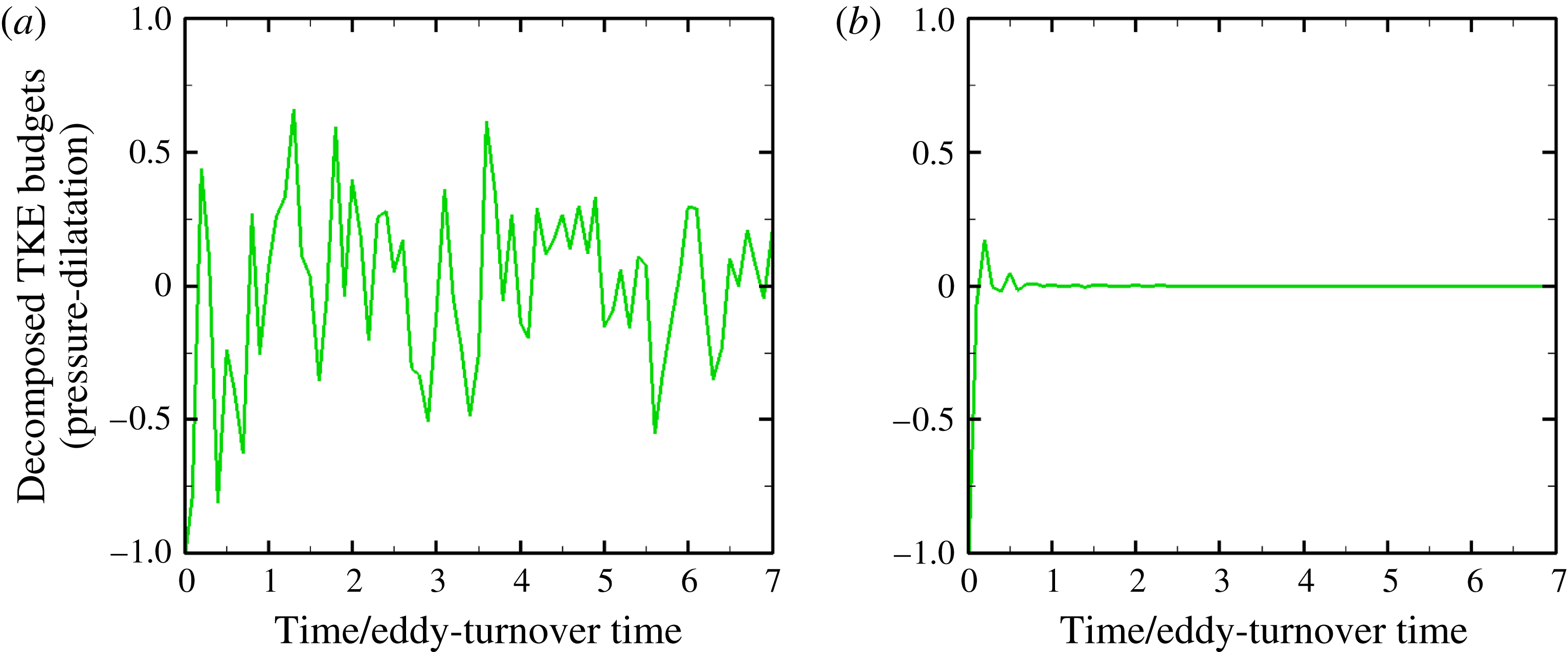
The right-hand side terms correspond to advection, component-wise pressure–dilatation, shear viscous dissipation and bulk viscous dissipation (Kida & Orszag Reference Kida and Orszag1992). Figures 13 and 14 show the contributions of each of the terms in (3.7) for both velocity components.
Time evolution of the decomposed turbulent kinetic energy budgets based on the solenoidal (a,b) and dilatational (c,d) fields for
 $\unicode[STIX]{x1D707}_{b}/\unicode[STIX]{x1D707}=0$
(a,c) and 1000 (b,d), without component-wise pressure–dilatation. Red: advection; blue: shear viscous dissipation; black: bulk viscous dissipation.

Time evolution of the component-wise pressure–dilatation for
 $\unicode[STIX]{x1D707}_{b}/\unicode[STIX]{x1D707}=0$
(a) and
 $1000$
(b).

These results clearly explain the effect of bulk viscosity on energy dissipation. The component-wise pressure–dilatation term is the same as for the full TKE; the shear and bulk dilatational damping observed in figure 12 primarily influence the dilatational kinetic energy, whereas the shear solenoidal dissipation affects the solenoidal kinetic energy. The crucial observation is that bulk viscous dissipation reduces the advection term (equal and opposite for solenoidal and dilatational) to a negligible contribution within a tenth of an eddy-turnover time. Since this term represents the only mechanism for solenoidal–dilatational exchanges, its reduction decouples solenoidal from dilatational modes. Consequently, the dissipation of the dilatational TKE due to the large bulk viscous dissipation, accompanied by a reduction in dilatation, leaves the solenoidal kinetic energy unaffected and dependent only on solenoidal dissipation – plus a minor contribution of bulk viscosity. In other words, bulk viscosity augments the effective viscous dissipation coefficient of the solenoidal TKE by a relatively small amount (see § 3.4), leaving enstrophy nearly unscathed. Given that the solenoidal and dilatational fields are uncorrelated, pseudo-sound theory (e.g. as in Ristorcelli Reference Ristorcelli1997) could be used to obtain additional insights into this problem.
A possible implication of these results is for compressible mixing layers, where compressibility has been shown to inhibit mixing (Papamoschou & Roshko Reference Papamoschou and Roshko1988). It is known that reduced turbulent production due to smaller pressure fluctuations is responsible for reduced mixing layer growth (Sarkar Reference Sarkar1995; Vreman et al. Reference Vreman, Sandham and Luo1996). Our results indicate that the solenoidal and dilatational motions are decoupled and that dilatation is greatly reduced by bulk viscous dissipation. We speculate that such a decoupling, perhaps by injecting a small amount of gas with large bulk viscosity, may be exploited to present strategies to overcome reductions in pressure fluctuations and thus improve mixing of compressible shear layers.
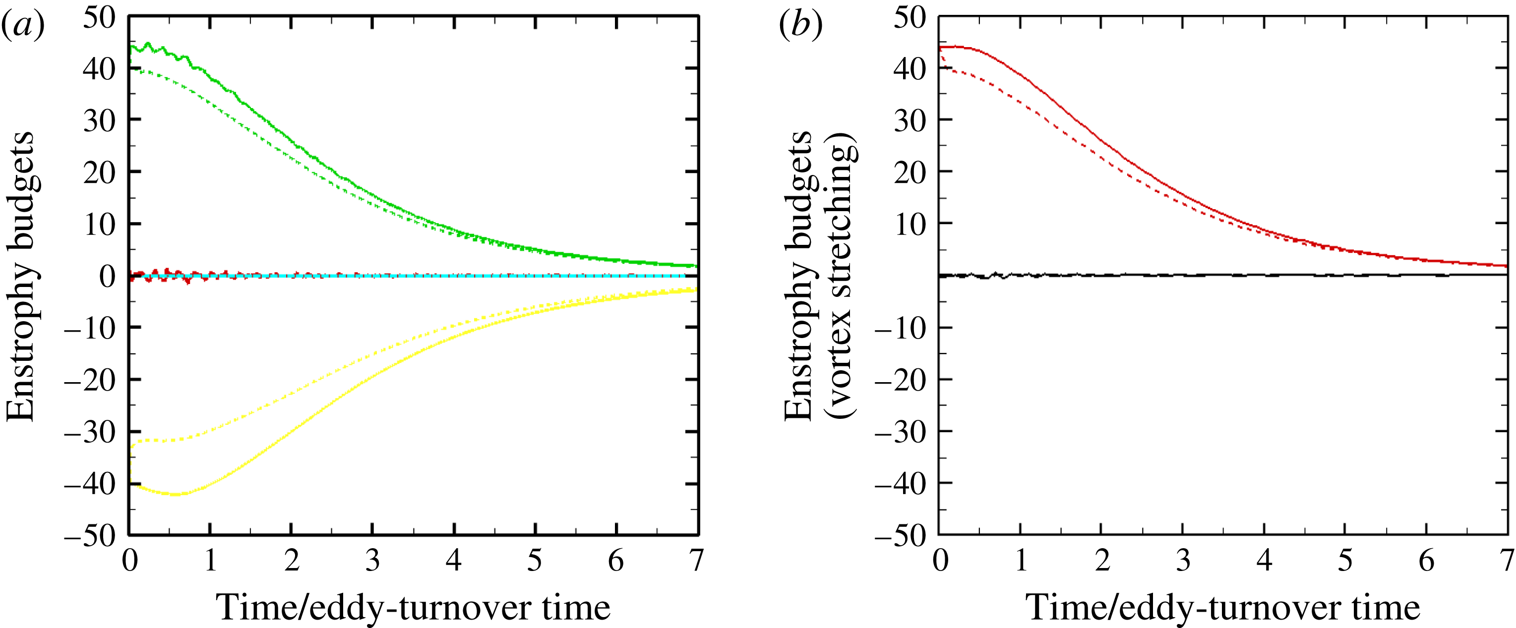
Time evolution of the enstrophy budgets for
 $\unicode[STIX]{x1D707}_{b}/\unicode[STIX]{x1D707}=0$
(solid) and 1000 (dotted). (a) Right-hand side of (3.8) (red: enstrophy dilatation; green: vortex stretching; blue: baroclinic vorticity; black shear viscous diffusion; yellow: shear-density gradient; cyan: bulk viscosity-density gradient; dashed); (b) vortex stretching term for the decomposed velocity fields (red: solenoidal; black: dilatational).

3.3.2 Enstrophy transport
The transport of enstrophy,
 $$\begin{eqnarray}\displaystyle \frac{\unicode[STIX]{x2202}\langle Q\rangle }{\unicode[STIX]{x2202}t} & = & \displaystyle \langle -Q\unicode[STIX]{x1D6E5}\rangle +\langle \unicode[STIX]{x1D74E}\boldsymbol{\cdot }\unicode[STIX]{x1D64E}\boldsymbol{\cdot }\unicode[STIX]{x1D74E}\rangle -\left\langle \frac{1}{\unicode[STIX]{x1D70C}^{2}}[\unicode[STIX]{x1D74E}\boldsymbol{\cdot }(\unicode[STIX]{x1D735}p\times \unicode[STIX]{x1D735}\unicode[STIX]{x1D70C})]\right\rangle +\frac{1}{Re}\left\langle \frac{1}{\unicode[STIX]{x1D70C}}\unicode[STIX]{x1D74E}\boldsymbol{\cdot }\unicode[STIX]{x1D6FB}^{2}\unicode[STIX]{x1D74E}\right\rangle \nonumber\\ \displaystyle & & \displaystyle -\,\frac{1}{Re}\left\langle \unicode[STIX]{x1D74E}\boldsymbol{\cdot }\left[\frac{1}{\unicode[STIX]{x1D70C}^{2}}\unicode[STIX]{x1D735}\unicode[STIX]{x1D70C}\times \left(\unicode[STIX]{x1D6FB}^{2}\boldsymbol{u}+\frac{1}{3}\unicode[STIX]{x1D735}\unicode[STIX]{x1D6E5}\right)-\frac{1}{\unicode[STIX]{x1D70C}^{2}}\frac{\unicode[STIX]{x1D707}_{b}}{\unicode[STIX]{x1D707}}\unicode[STIX]{x1D735}\unicode[STIX]{x1D70C}\times \unicode[STIX]{x1D735}\unicode[STIX]{x1D6E5}\right]\right\rangle ,\end{eqnarray}$$
where
 $Q=\unicode[STIX]{x1D74E}\boldsymbol{\cdot }\unicode[STIX]{x1D74E}/2$
, provides useful insight into the vortex dynamics. The right-hand side terms correspond to enstrophy dilatation, vortex stretching, baroclinic vorticity, shear viscous diffusion and, in the brackets, shear-density gradient and bulk viscosity-density gradients. The contributions of these terms are shown in figure 15(a), as well as the vortex stretching terms after Helmholtz decomposition only (b). The enstrophy dynamics is dominated by vortex stretching (production) and shear-density gradient (destruction). Bulk viscosity effectively reduces the magnitude of destruction by
 ${\sim}10\,\%$
, and production by
 ${\sim}20\,\%$
. Other terms are essentially negligible. Helmholtz decomposition can be used to distinguish between the solenoidal and dilatational contributions to vortex stretching. In particular, decomposing the vortex stretching term into solenoidal and dilatational components,
 $\langle \unicode[STIX]{x1D74E}\boldsymbol{\cdot }\unicode[STIX]{x1D64E}^{(s)}\boldsymbol{\cdot }\unicode[STIX]{x1D74E}\rangle +\langle \unicode[STIX]{x1D74E}\boldsymbol{\cdot }\unicode[STIX]{x1D64E}^{(d)}\boldsymbol{\cdot }\unicode[STIX]{x1D74E}\rangle$
(figure 15
b), clearly shows that the major contribution of vortex stretching comes from the solenoidal velocity component, which mirrors the total vortex stretching term in (3.8). On the other hand, the dilatational contribution to vorticity dynamics is negligible.
3.4 Spectral and probability density function analysis
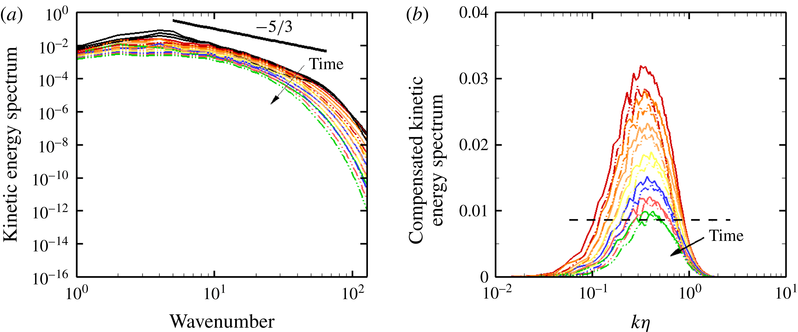
Now that the energy transfer and dissipation mechanisms are understood, we turn to spectra and probability density functions (PDFs) to evaluate the energetics across scales. The TKE spectra at the first seven eddy-turnover times are shown in figure 16. Overall, bulk viscosity damps all scales, with a more pronounced effect at the highest wavenumbers. Compensated spectra show a plateau for
 $0.3\lesssim k\unicode[STIX]{x1D702}\lesssim 0.5$
. However, the exact effect of bulk viscosity on the energy contents at different scales is difficult to ascertain beyond these observations. We note that past high-resolution simulations showed a
 $k^{-2}$
scaling of the spectrum in the inertial range for supersonic turbulence (Kritsuk et al.
Reference Kritsuk, Norman, Padoan and Wagner2007) and in the presence of large-scale shocks (Chen et al.
Reference Chen, Xia, Wang and Yang2015).
Turbulent kinetic energy spectra (a) and compensated spectra (b) at the first seven eddy-turnover times for
 $\unicode[STIX]{x1D707}_{b}/\unicode[STIX]{x1D707}=0$
(solid) and 1000 (dash-dot).

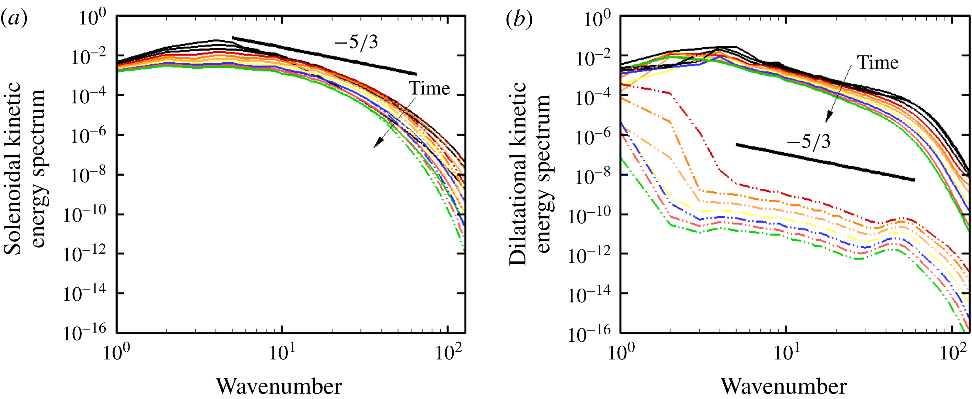
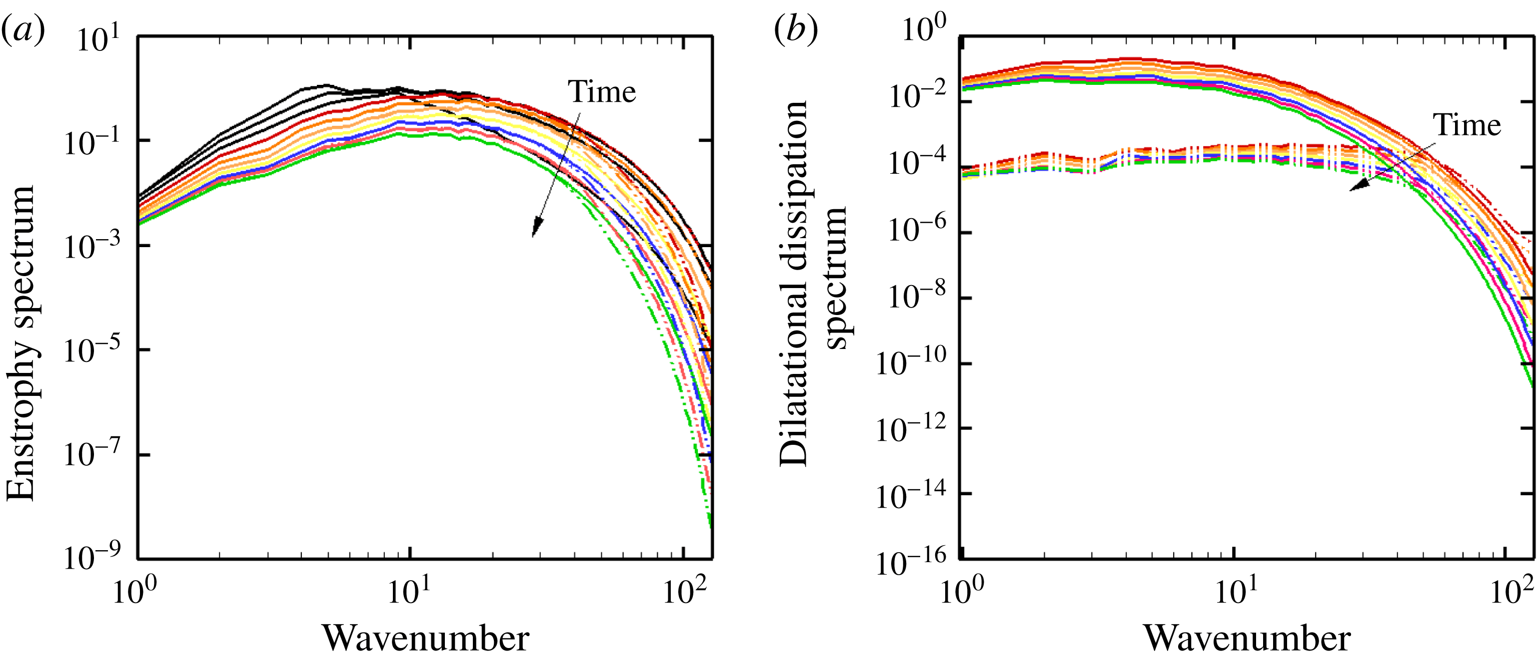
Decomposing the kinetic energy spectra into solenoidal and dilatational components clarifies the effect of bulk viscosity on the energy contents across scales. Figure 17 shows the decomposed TKE spectra, and figure 18 the enstrophy and dilatational dissipation. For the solenoidal contribution, the addition of bulk viscosity minimally increases dissipation, only at high wavenumbers (
 $k\gtrsim 32$
). In other words, bulk viscosity augments the viscous dissipation coefficient, thus increasing the dissipation range, consistent with the previous observations. This behaviour holds for both the solenoidal TKE and enstrophy spectra.
Solenoidal (a) and dilatational (b) turbulent kinetic energy spectra at the first seven eddy-turnover times for
 $\unicode[STIX]{x1D707}_{b}/\unicode[STIX]{x1D707}=0$
(solid) and 1000 (dash-dot).

Enstrophy (a) and dilatational dissipation (b) spectra at the first seven eddy-turnover times for
 $\unicode[STIX]{x1D707}_{b}/\unicode[STIX]{x1D707}=0$
(solid) and 1000 (dash-dot).

For the dilatational component, the spectra are decreased by several decades in the presence of bulk viscosity. A relatively flat dilatational dissipation spectrum is achieved, before falling off at the highest wavenumbers, indicating that dilatational dissipation affects large and intermediate scales (
 $k\lesssim 32$
), with essentially no influence on the small scales. Consequently, the largest dilatational eddy motions contain less energy than their solenoidal counterparts. In the presence of bulk viscosity, an upward turn in the dilatational energy spectrum is observed at high wavenumbers; the results suggest that the kinetic energy dissipation at small scales cannot keep up with the increased dissipation at large to intermediate scales, thus leading to what appears to be energy pile up. In addition, intermediate scales are directly damped, by several decades, initially for
 $4\lesssim k\lesssim 30$
; this range shifts left over time. The slope is closer to
 $-5/3$
than the simulations with
 $\unicode[STIX]{x1D707}_{b}=0$
. With no bulk viscosity, the spectra are comparable to those corresponding to solenoidal dissipation.
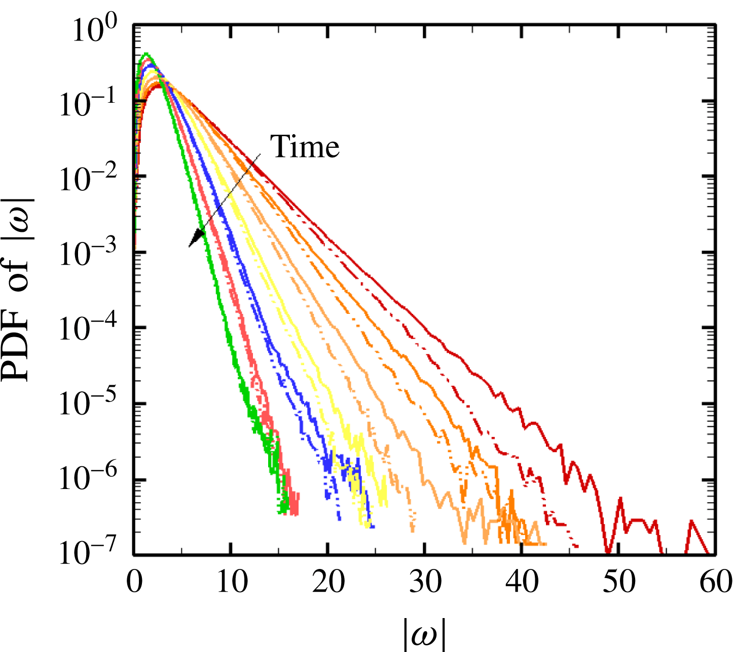
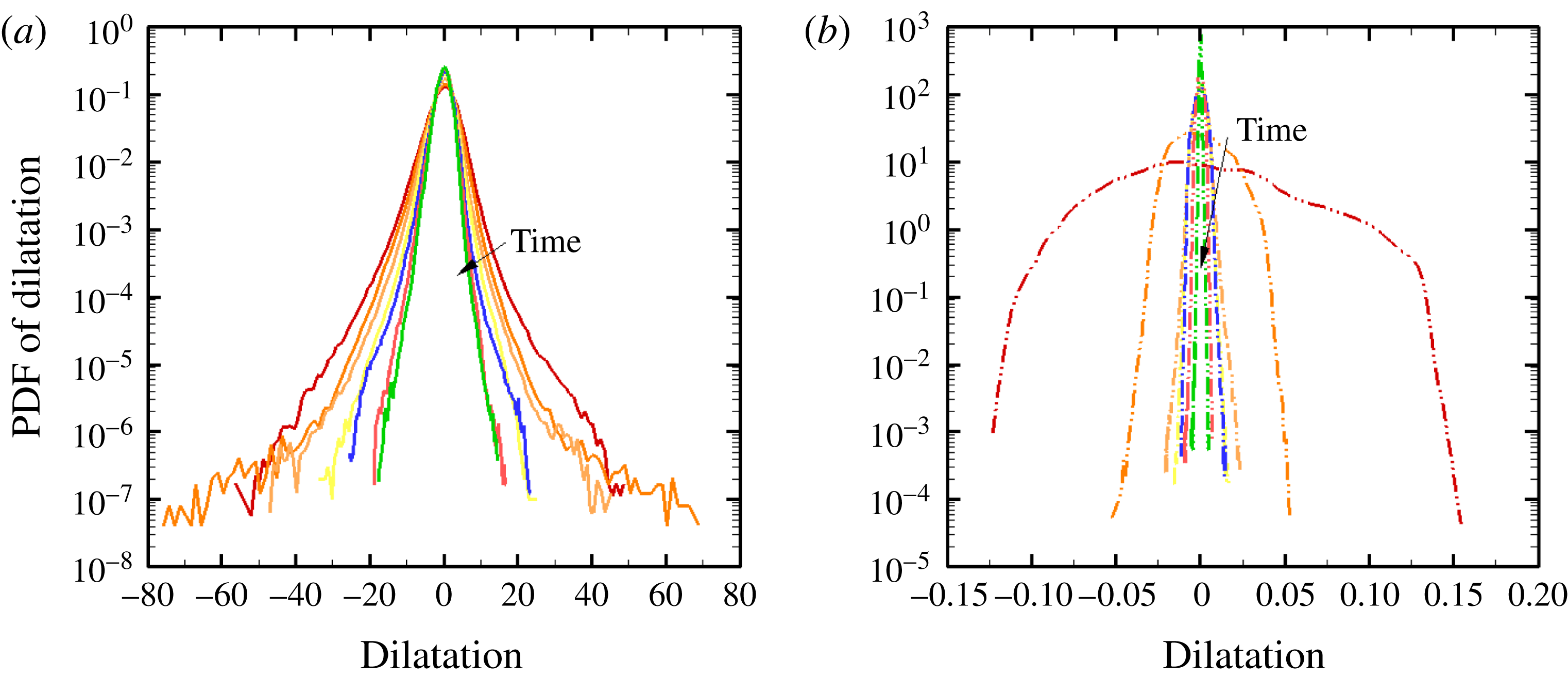
The PDF of the vorticity magnitude is shown in figure 19. As time evolves, the peak shifts to the left as a result of viscous dissipation. For large magnitudes, the PDF exhibits a power-law behaviour. The effect of bulk viscosity is evident only at large magnitudes, in which case it reduces the slope. As expected, the PDF of dilatation (figure 20) exhibits high sensitivity to bulk viscosity. Consistent with past work (Wang et al. Reference Wang, Shi, Wang, Xiao, He and Chen2012), compressions are slightly more likely to occur than expansions in compressible turbulence (with no bulk viscosity). In the presence of bulk viscosity, a relatively flat distribution is observed after approximately four eddy-turnover times although it leans to the right slightly, indicating that expansions are more likely to occur than compressions. This phenomenon may be caused by dilatational dissipation, in which higher compressions undergo greater dissipation (Chen et al. Reference Chen, Xia, Wang and Yang2015).
Time evolution of the PDF of vorticity for
 $\unicode[STIX]{x1D707}_{b}/\unicode[STIX]{x1D707}=0$
(solid) and 1000 (dash-dot).

Time evolution of the PDF of dilatation for
 $\unicode[STIX]{x1D707}_{b}/\unicode[STIX]{x1D707}=0$
(a) and 1000 (b).

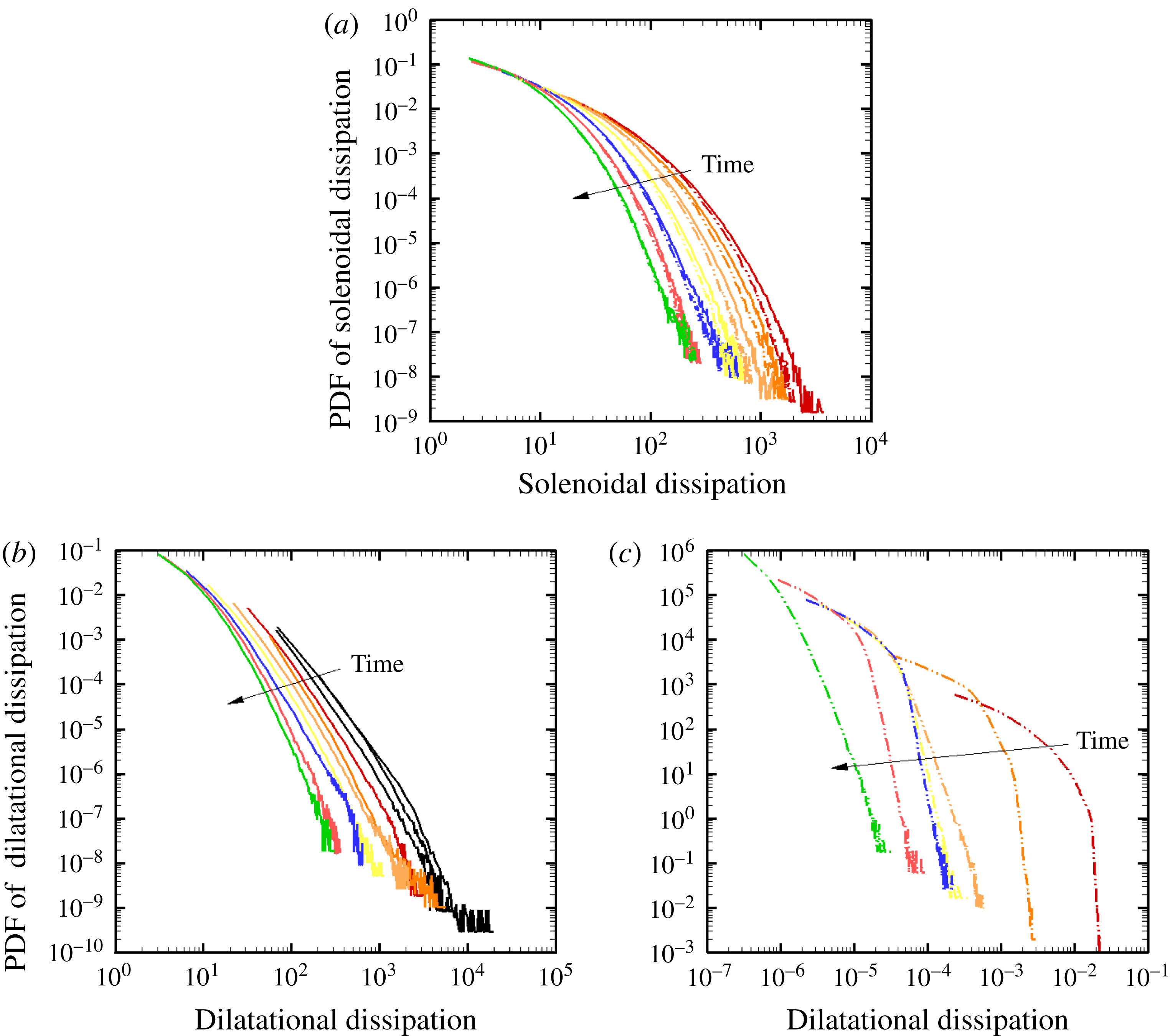
The PDFs of the Helmholtz decomposed dissipation rate are shown in figure 21 and are consistent with the above results. In all cases, the distributions shift toward the right as time evolves. As expected, bulk viscosity has little effect on the solenoidal dissipation rate; a power-law distribution is observed. On the other hand, bulk viscosity significantly affects the PDF of the dilatational dissipation rate, and reduces the slope at large magnitudes. The dilatational dissipation rate follows a power law when
 $\unicode[STIX]{x1D707}_{b}=0$
. The region of low dissipation rate is wide and drops off quickly at early times; at late times, the PDF of dilatational dissipation recovers a power-law-like shape. With bulk viscosity, the magnitudes of the dilatational PDF is several orders of magnitude smaller.
PDF of the solenoidal (a) and dilatational (b:
 $\unicode[STIX]{x1D707}_{b}/\unicode[STIX]{x1D707}=0$
; c:
 $\unicode[STIX]{x1D707}_{b}/\unicode[STIX]{x1D707}=1000$
) dissipation.

3.5 Turbulent Mach number dependence
As discussed in § 1, equation (1.2) indicates that the relative importance of bulk to shear viscous dissipation depends on the bulk to shear viscosity ratio, as well as on a measure of volumetric to deviatoric deformation rates, e.g.
 $\unicode[STIX]{x1D6E5}^{2}/\unicode[STIX]{x1D61A}_{ij}^{(d)}\unicode[STIX]{x1D61A}_{ij}^{(d)}$
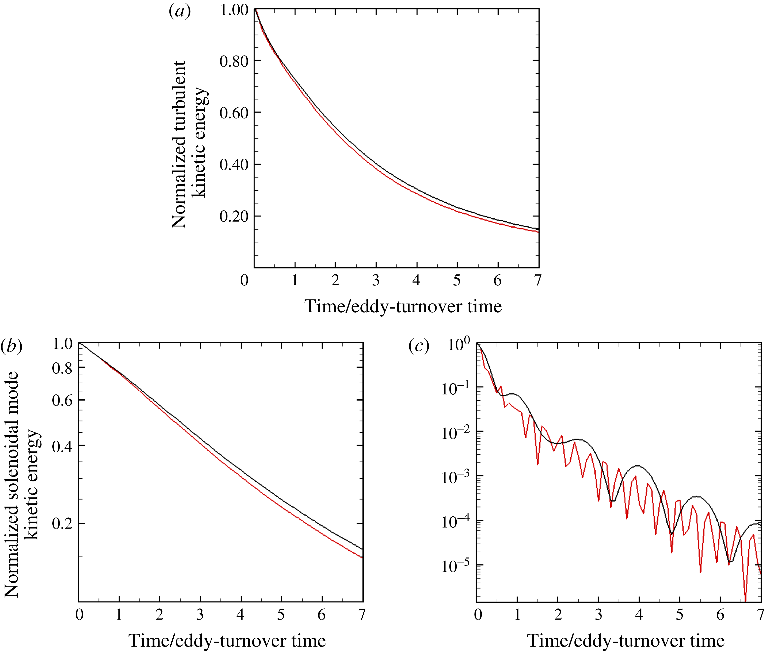
. The present study was designed to investigate the former, held constant in this study. Although a comprehensive study of the latter falls beyond the scope of this work, we discuss here how the mean compressibility of the flow, quantified by the initial turbulent Mach number, affects the dynamics. Figure 22 shows the time evolution of the normalized turbulent kinetic energy (total and decomposed) and figure 23 shows the time evolution of the turbulent kinetic energy budgets based on the solenoidal and dilatational fields, for initial turbulent Mach numbers
 $M_{t}=0.1$
and 0.4, with
 $\unicode[STIX]{x1D707}_{b}/\unicode[STIX]{x1D707}=1000$
.
Time evolution of the normalized total (a), solenoidal (b, semilog) and dilatational (c, semilog) turbulent kinetic energy (top) for initial turbulent Mach numbers
 $M_{t}=0.1$
(red) and
 $0.4$
(black), with
 $\unicode[STIX]{x1D707}_{b}/\unicode[STIX]{x1D707}=1000$
.

Time evolution of the turbulent kinetic energy budgets based on the solenoidal (a,c) and dilatational (b,d) fields for initial turbulent Mach numbers
 $M_{t}=0.1$
(a,b) and
 $0.4$
(c,d), with
 $\unicode[STIX]{x1D707}_{b}/\unicode[STIX]{x1D707}=1000$
. Red: advection; blue: shear viscous dissipation; black: bulk viscous dissipation; green: component-wise pressure–dilatation.

Minor differences are observed in the turbulent kinetic energy evolution with different initial turbulent Mach numbers. When considering the decomposed budgets, the only notable differences lie in the component-wise pressure–dilatation. The reason for this lack of difference is that the turbulent Mach numbers at the time when bulk viscosity is introduced, 0.07 for the
 $M_{t}=0.1$
case and 0.25 for the
 $M_{t}=0.4$
case, do not give rise to significant differences in the energy transfer mechanisms.
We note that the current simulations set-up renders fair comparisons between different Mach numbers difficult. As described in § 2.2, the initial random flow is evolved over three eddy-turnover times before bulk viscosity is introduced. Our approach to investigate
 $M_{t}$
dependence was to change the initial turbulence intensity to achieve the appropriate initial turbulent Mach number, while keeping the Reynolds number the same; at the time when bulk viscosity was introduced
 $Re_{\unicode[STIX]{x1D706}}\approx 55.6$
for the
 $M_{t}=0.1$
case and 52.3 for the
 $M_{t}=0.4$
case, leading to similar flow conditions. For this reason, the period of the oscillations produced by the initially generated acoustic waves and visible in the dilatational budget and component-wise pressure–dilatation is different. We further note that we sought to keep the turbulent Mach number sufficiently low such that shocklets were not generated. A comprehensive study of the combined effect of bulk viscosity and compressibility would require a different problem set-up and thus lies beyond the scope of the present work; we will pursue this direction in a future effort.
4 Conclusions
We used DNS to investigate the role of bulk viscosity on the decay of compressible, homogeneous, isotropic turbulence. We considered ratios of bulk to shear viscosities of 0, 30 and 1000 corresponding to values reported in the literature for monatomic gases,
 $\text{H}_{2}$
and
 $\text{CO}_{2}$
, respectively. This parametric study, supported by a Helmholtz decomposition of the velocity field, enabled a better understanding of the effect of bulk viscosity on compressible turbulence.
Our simulations demonstrate that bulk viscosity increases the decay rate of turbulent kinetic energy. While enstrophy exhibits little sensitivity to bulk viscosity, dilatation is reduced by over two orders of magnitude within the first two eddy-turnover times. To identify the responsible mechanisms, we performed a Helmholtz decomposition of the flow. The data demonstrated that increasing bulk viscosity significantly damps the dilatational velocity field – and thus dilatation – by increasing bulk dilatational dissipation. As a result, exchanges between dilatational and solenoidal modes are inhibited, such that solenoidal motions remain essentially unaffected by bulk viscosity. In short, bulk viscosity renders compressible turbulence incompressible by reducing energy transfer between translational and internal energy. The skewness and flatness of the velocity derivatives are also indicative that a state of essentially incompressible turbulence has been achieved.
Dilatational modes are damped by bulk viscous stresses at large to moderate scales (
 $k\lesssim 32$
); bulk dilatational dissipation leaves the small-scale dynamics essentially unchanged. As a result, the range of influence of the turbulence is enlarged. By contrast, for the solenoidal contribution, the effective viscous dissipation coefficient is increased by bulk viscosity and thus affects the small scales only. Furthermore, the probability density function indicates that compressions are more likely than expansions.
For gases such as air whose bulk viscosity is of the order of its shear viscosity, the turbulence is not expected to be significantly affected by bulk viscosity. Thus, neglecting bulk viscosity is likely to produce acceptable results. However, in problems involving compressible flows of
 $\text{CO}_{2}$
(e.g. Mars entry, certain combustion applications) and other gases with large
 $\unicode[STIX]{x1D707}_{b}/\unicode[STIX]{x1D707}$
, attention must be paid to accounting for bulk viscosity. While this work constitutes the first systematic study of the role of bulk viscosity on the decay of compressible, homogeneous, isotropic turbulence, it is restricted by the assumptions made therein. For instance, the dependence of the flow on the initial turbulent Mach number and that of
 $\unicode[STIX]{x1D707}_{b}$
on frequency were beyond the scope of this article. In particular, as the turbulent Mach number is increased, eddy shocklets may be generated (Samtaney et al.
Reference Samtaney, Pullin and Kosovic2001), giving rise to regions of increased dilatation likely to be sensitive to bulk viscous damping. We are planning follow-up studies precisely to investigate these effects.
Acknowledgements
The authors gratefully acknowledge helpful discussions with Professors V. Raman and D. Dowling. This work used the Extreme Science and Engineering Discovery Environment (XSEDE), which is supported by National Science Foundation grant no. ACI-1548562 (Towns et al. Reference Towns, Cockerill, Dahan, Foster, Gaither, Grimshaw, Hazlewood, Lathrop, Lifka and Peterson2014).