1 Introduction
The advancement of computing hardware and the advent of parallel computing algorithms have enabled unprecedented insight into complex flow physics using computational fluid dynamics (CFD). This insight is often crucial in developing a detailed understanding of multi-disciplinary interactions with complex flow environments. However, the computational cost associated with high-fidelity analysis tools has prevented their integration into broad systems-level and multi-disciplinary studies. This critical need has motivated the pursuit of tractable, accurate and robust reduced-order models (ROMs).
A commonly used ROM approach involves projecting the governing equations onto a reduced-dimensional space comprising characteristic bases (Noack & Eckelmann Reference Noack and Eckelmann1994; Noack et al. Reference Noack, Afanasiev, Morzynski, Tadmor and Thiele2003; Rowley Reference Rowley2005; Ilak et al. Reference Ilak, Bagheri, Brandt, Rowley and Henningson2010; Holmes et al. Reference Holmes, Lumley, Berkooz and Rowley2012; Kalashnikova et al. Reference Kalashnikova, van Bloemen, Arunajatesan and Barone2014). The projections can be orthogonal (e.g. Galerkin) or non-orthogonal (e.g. Petrov–Galerkin) (Noack & Eckelmann Reference Noack and Eckelmann1994; Noack et al. Reference Noack, Afanasiev, Morzynski, Tadmor and Thiele2003; Rowley Reference Rowley2005; Ilak et al. Reference Ilak, Bagheri, Brandt, Rowley and Henningson2010; Holmes et al. Reference Holmes, Lumley, Berkooz and Rowley2012; Kalashnikova et al. Reference Kalashnikova, van Bloemen, Arunajatesan and Barone2014). The accuracy of such approaches is intimately bound to the quality of the chosen bases. The data from which appropriate bases for unsteady flow fields can be extracted are typically limited to small spatial and temporal domains due to the previously mentioned computational expense of high-fidelity CFD analyses. Furthermore, such data are high-dimensional due to the spatial and temporal resolution typically required for high-fidelity analyses. Thus, identification of a compact set of dynamically important flow features that fundamentally characterise the fluid dynamics is a non-trivial exercise. Proper orthogonal decomposition (POD), or principal components analysis (PCA) (Sirovich Reference Sirovich1987; Berkooz, Holmes & Lumley Reference Berkooz, Holmes and Lumley1993; Chatterjee Reference Chatterjee2000; Lucia, Beran & Silva Reference Lucia, Beran and Silva2004; Holmes et al. Reference Holmes, Lumley, Berkooz and Rowley2012), is a widely used and explored technique aimed at meeting this need. The approach is based on identifying and ordering principal components in observed data. The POD modes are optimal in terms of capturing the energy of an observed flow response; thus, a reduced-dimensional basis of the system is identified by truncating the modes based on the energy contribution to the response (Sirovich Reference Sirovich1987; Berkooz et al. Reference Berkooz, Holmes and Lumley1993; Chatterjee Reference Chatterjee2000; Lucia et al. Reference Lucia, Beran and Silva2004; Holmes et al. Reference Holmes, Lumley, Berkooz and Rowley2012). However, there are several issues with this approach. First, the POD modes are only optimal in the sense of reconstructing the observed flow responses (Ilak & Rowley Reference Ilak and Rowley2008; Holmes et al. Reference Holmes, Lumley, Berkooz and Rowley2012; Balajewicz, Dowell & Noack Reference Balajewicz, Dowell and Noack2013). Thus, they may not generalise well for model predictions that deviate from observed conditions. From a fluid physics perspective, truncation in the first few most energetic modes is problematic due to energy exchange between large- and small-scale structures (Amsallem & Farhat Reference Amsallem and Farhat2012; Holmes et al. Reference Holmes, Lumley, Berkooz and Rowley2012; Balajewicz et al. Reference Balajewicz, Dowell and Noack2013). The large-scale structures are formed as a result of disturbances in the flow – obtaining energy from the mean flow and then subsequently breaking down into smaller scales (Pope Reference Pope2009). The small-scale structures then cause energy dissipation and result in viscosity in the fluid flow. Thus, the POD based Galerkin ROMs that use a truncated basis may overpredict the kinetic energy due to insufficient energy dissipation (Noack, Papas & Monkewitz Reference Noack, Papas and Monkewitz2005; Amsallem & Farhat Reference Amsallem and Farhat2012; Holmes et al. Reference Holmes, Lumley, Berkooz and Rowley2012; Balajewicz et al. Reference Balajewicz, Dowell and Noack2013). Moreover, the energy accumulation over a period of time may also cause the ROM to become unstable (Amsallem & Farhat Reference Amsallem and Farhat2012; Amsallem, Zahr & Farhat Reference Amsallem, Zahr and Farhat2012; Balajewicz et al. Reference Balajewicz, Dowell and Noack2013). Related to this, it is now well established that POD modes are ineffective in capturing the local dynamics (or transience) of full-order systems unless a large number of modes are used (Ilak & Rowley Reference Ilak and Rowley2008; Balajewicz et al. Reference Balajewicz, Dowell and Noack2013). This is because a set of POD modes minimises reconstruction errors over the entire time history of training data, and may not capture low-energy dynamically important transience. For these reasons, the optimality of POD is generally not a well-suited criterion for model reduction of nonlinear unsteady flows.
Techniques such as balanced truncation (Zhou, Doyle & Glover Reference Zhou, Doyle and Glover1996), balanced POD (BPOD) (Ilak et al. Reference Ilak, Bagheri, Brandt, Rowley and Henningson2010) and the eigensystem realisation algorithm (ERA) (Ma, Ahuja & Rowley Reference Ma, Ahuja and Rowley2010) have addressed some of the limitations identified earlier. However, balanced truncation is intractable for large data (for more than 10 000 degrees of freedom) (Kalashnikova et al. Reference Kalashnikova, van Bloemen, Arunajatesan and Barone2014), BPOD is only applicable to response data of linear systems as it requires adjoint system information (Ilak et al. Reference Ilak, Bagheri, Brandt, Rowley and Henningson2010; Ma et al. Reference Ma, Ahuja and Rowley2010), and modes generated by the ERA cannot be used for projection of nonlinear dynamics (Ma et al. Reference Ma, Ahuja and Rowley2010). In a recent study, a technique was developed to generate a stable Galerkin projection based ROM (Balajewicz et al. Reference Balajewicz, Dowell and Noack2013). However, this requires an iterative process that involves multiple time integrations of the ROM until an energy balance is achieved. These issues highlight the need to explore alternative basis identification techniques that not only generalise well to changing flow conditions but also accurately capture essential multi-scale features.
Olshausen & Field (Reference Olshausen and Field1996) argue that most naturally occurring phenomena are conveniently represented using non-Gaussian distributions, whereas the PCA approach is suitable when the structure of the data can be represented using Gaussian distributions. In Gaussian distributions, the linear correlation between statistical structures is the most important relation. Observations from a naturally occurring phenomenon, such as natural images, contain higher-order statistics. To this end, a technique based on sparse coding was proposed to extract the higher-order features from natural image data (Olshausen & Field Reference Olshausen and Field1996). This approach, which is also referred to as sparse dictionary learning (Kreutz-Delgado et al. Reference Kreutz-Delgado, Murray, Rao, Engan, Lee and Sejnowski2003), generates a finite dictionary of modes in which only a subset is active for a given time window. Furthermore, sparse coding describes a nonlinear system in a locally linear manner by tailoring the modes to the local behaviour of the system (Yang, Yu & Huang Reference Yang, Yu and Huang2010). Thus, compared with the POD approach, where the principal components of the observed data are identified, ordered and then truncated to a compact set, sparse coding is formulated as a procedure to identify a compact representation that approximately spans all of the observed data. The sparse coding approach has been successfully applied in a number of topics, such as in image processing (Yang et al. Reference Yang, Yu, Gong and Huang2009), audio analysis (Grosse et al. Reference Grosse, Raina, Kwong and Ng2012), neuroscience (Olshausen & Field Reference Olshausen and Field1996, Reference Olshausen and Field2004; Lee et al. Reference Lee, Battle, Raina and Ng2006) and electrical power disaggregation (Kolter, Batra & Ng Reference Kolter, Batra and Ng2010). Recently, a sparsity-promoting dynamic mode decomposition (DMD) algorithm was used to carry out efficient and accurate reconstruction of fluid-flow data (Jovanović, Schmid & Nichols Reference Jovanović, Schmid and Nichols2014). However, to the best of the authors’ knowledge, the sparse coding approach has not been examined for reduced-order modelling of dynamical systems.
The overall objective of this study is to explore the concepts of sparse coding for the purposes of identifying coherent global and local structures in unsteady flows, and the development of robust and accurate ROMs for predicting unsteady flow field behaviour. The specific objectives of the paper are to (1) develop a framework that combines concepts of sparse coding with a Galerkin based projection methodology in order to generate predictive ROMs for unsteady flow fields and (2) investigate the performance of the ROMs for incompressible flow in a two-dimensional (2-D) lid-driven cavity.
The remainder of this paper is organised as follows. The POD and sparse coding approaches are presented in § 2. Application of POD and sparse modes to model the lid-driven cavity is presented in § 3. Concluding remarks are given in § 4.
2 Method of solution
High-resolution data are computed by solving the 2-D incompressible Navier–Stokes (NS) equations using a direct numerical simulation (DNS) CFD solver. The POD approach is based on the method of snapshots developed by Sirovich (Reference Sirovich1987). Sparse modes are computed using the algorithm developed by Friedman, Hastie & Tibshirani (Reference Friedman, Hastie and Tibshirani2010). These approaches are detailed next.
2.1 Full-order model
The DNS solution to the non-dimensionalised NS equations given by (2.1) is generated using an immersed-boundary method (Mittal et al. Reference Mittal, Dong, Bozkurttas, Najjar, Vargas and von Loebbecke2008),
 $$\begin{eqnarray}\unicode[STIX]{x1D735}\boldsymbol{\cdot }\boldsymbol{u}=0,\quad \frac{\unicode[STIX]{x2202}\boldsymbol{u}}{\unicode[STIX]{x2202}t}+(\boldsymbol{u}\boldsymbol{\cdot }\unicode[STIX]{x1D735})\boldsymbol{u}=-\unicode[STIX]{x1D735}p+\frac{1}{Re}\unicode[STIX]{x1D6FB}^{2}\boldsymbol{u},\end{eqnarray}$$
where
 $\unicode[STIX]{x1D735}$
is the gradient operator,
 $t$
is the non-dimensional time,
 $Re$
is the Reynolds number,
 $p$
is the non-dimensional pressure and
 $\boldsymbol{u}$
is the non-dimensional velocity. The non-dimensionalisation is carried out as
 $$\begin{eqnarray}\boldsymbol{x}={\displaystyle \frac{\boldsymbol{x}^{\ast }}{L}},\quad \boldsymbol{u}={\displaystyle \frac{\boldsymbol{u}^{\ast }}{u_{0}}},\quad t={\displaystyle \frac{t^{\ast }}{(L/u_{0})}},\quad p={\displaystyle \frac{p^{\ast }}{\unicode[STIX]{x1D70C}{u_{0}}^{2}}},\end{eqnarray}$$
where
 $\boldsymbol{x}$
is the non-dimensional position vector,
 $L$
is the characteristic length,
 $\unicode[STIX]{x1D70C}$
is the density and
 $u_{0}$
is the characteristic velocity. The dimensional quantities are represented with superscript asterisks. The DNS code uses a second-order central-difference spatial scheme and a second-order fractional-step method for time marching. The equations are discretised on a Cartesian mesh and boundary conditions are imposed using a ghost-cell procedure (Mittal et al.
Reference Mittal, Dong, Bozkurttas, Najjar, Vargas and von Loebbecke2008).
2.2 Modal decompositions
The full-order solution is decomposed into mean,
 $\bar{\boldsymbol{U}}(\boldsymbol{x})$
, and fluctuating components,
 $\boldsymbol{q}(\boldsymbol{x},t)$
, of the velocity. The component
 $\bar{\boldsymbol{U}}(\boldsymbol{x})$
is evaluated as the time average of the velocity field. The component
 $\boldsymbol{q}(\boldsymbol{x},t)$
is approximated as a linear combination of modes:
 $$\begin{eqnarray}\boldsymbol{q}(\boldsymbol{x},t)=\tilde{\boldsymbol{u}}(\boldsymbol{x},t)\approx \mathop{\sum }_{i=1}^{N}s^{i}(t)\unicode[STIX]{x1D731}_{i}(\boldsymbol{x}),\end{eqnarray}$$
where
 $\unicode[STIX]{x1D731}_{i}$
is the
 $i\text{th}$
mode,
 $\tilde{u}$
is the fluctuating component of the velocity field,
 $N$
is the number of modes,
 $s^{i}(t)$
is the coefficient corresponding to the
 $i$
th mode at time
 $t$
and
 $x\in \unicode[STIX]{x1D6FA}$
,
 $\unicode[STIX]{x1D6FA}$
being the flow domain. The inner product between any vectors
 $\boldsymbol{f}$
and
 $\boldsymbol{g}$
in the vector space spanned by the modes is given as
 $$\begin{eqnarray}(\boldsymbol{f},\boldsymbol{g})=\int _{\unicode[STIX]{x1D6FA}}\boldsymbol{f}\boldsymbol{\cdot }\boldsymbol{g}\,\text{d}\unicode[STIX]{x1D6FA}.\end{eqnarray}$$
The inner product (2.4) is a standard energy product that conserves the energy in incompressible flows (Holmes et al. Reference Holmes, Lumley, Berkooz and Rowley2012). The computation of POD and sparse modes is discussed next.
2.2.1 Proper orthogonal decomposition
First, a snapshot matrix
 $\unicode[STIX]{x1D64C}=[\boldsymbol{q}_{1}\boldsymbol{q}_{2}\cdots \boldsymbol{q}_{k}\cdots \boldsymbol{q}_{m}]$
is constructed by stacking the flow observations
 $\boldsymbol{q}_{k}$
in its columns. Here, the observations are grid-independent, i.e. quantities at each of the grid points are multiplied by the corresponding cell volume. The procedure to extract POD modes from a snapshot matrix is extensively documented in Sirovich (Reference Sirovich1987) and Berkooz et al. (Reference Berkooz, Holmes and Lumley1993), and therefore is not repeated here. However, for comparative discussion with the sparse coding procedure, it should be noted that the POD modes fundamentally represent the solution to the following minimisation problem (Abdi & Williams Reference Abdi and Williams2010):
 $$\begin{eqnarray}\min _{\unicode[STIX]{x1D731},\unicode[STIX]{x1D64E}}\frac{1}{2}\Vert \unicode[STIX]{x1D64C}-\unicode[STIX]{x1D731}\unicode[STIX]{x1D64E}\Vert _{F}^{2},\quad \text{such that }(\unicode[STIX]{x1D731}_{i},\unicode[STIX]{x1D731}_{j})=\left\{\begin{array}{@{}ll@{}}1,\quad & i=j,\\ 0,\quad & i\neq j,\end{array}\right.\end{eqnarray}$$
where the columns of
 $\unicode[STIX]{x1D731}$
,
 $\unicode[STIX]{x1D731}_{i}$
are the POD modes,
 $\unicode[STIX]{x1D64E}$
is the coefficient matrix and
 $\Vert \cdot \Vert _{F}^{2}$
is the grid-independent square Frobenius norm of ‘
 $\cdot$
’. The objective function in (2.5) provides the error in the representation of the snapshot matrix by the modes
 $\unicode[STIX]{x1D731}$
. It should be noted that the POD modes are optimal in representing the snapshot matrix, i.e. a set of POD modes provides the smallest possible value for the objective function when compared with any other sets of the same size. Consequentially, the complete set of POD modes exactly reproduces the snapshot matrix (Holmes et al.
Reference Holmes, Lumley, Berkooz and Rowley2012). Moreover, the POD modes are orthogonal and are arranged in descending order of eigenvalues, where the first few modes represent the most energetic structures in the snapshot data (Berkooz et al.
Reference Berkooz, Holmes and Lumley1993).
2.2.2 Sparse coding
One approach to sparse coding is the solution of the following minimisation problem:
 $$\begin{eqnarray}\min _{\unicode[STIX]{x1D64E},\unicode[STIX]{x1D731}}\frac{1}{2}\Vert \unicode[STIX]{x1D64C}-\unicode[STIX]{x1D731}\unicode[STIX]{x1D64E}\Vert _{F}^{2}+\unicode[STIX]{x1D6FD}\Vert \unicode[STIX]{x1D64E}\Vert _{0},\quad \Vert \unicode[STIX]{x1D731}_{i}\Vert =1\quad \text{for all }i,\end{eqnarray}$$
where the columns of
 $\unicode[STIX]{x1D731}$
are the sparse modes,
 $\unicode[STIX]{x1D64E}$
is a matrix of activation coefficients, each column
 $\boldsymbol{s}_{k}$
of
 $\unicode[STIX]{x1D64E}$
is encouraged to be sparse by a penalty on the L0 ‘norm’ of
 $\unicode[STIX]{x1D64E}$
(the count of the non-zero elements of the matrix) and
 $\unicode[STIX]{x1D6FD}>0$
is the regularisation (or penalty) parameter, denoted here as the sparsity coefficient. It should be noted that if the penalty term is ignored, (2.6) reduces to the PCA problem (2.5) and yields the POD modes. The L0 penalty forces some of the entries in
 $\boldsymbol{s}_{k}$
to be zero, thereby resulting in a sparse coefficient matrix. The level of sparsity is controlled using
 $\unicode[STIX]{x1D6FD}$
, where increasing the value of
 $\unicode[STIX]{x1D6FD}$
increases the number of zero entries in
 $\boldsymbol{s}_{k}$
, thus producing a sparser coefficient matrix
 $\unicode[STIX]{x1D64E}$
. Yang et al. (Reference Yang, Yu, Gong and Huang2009) recommend that a value of
 $0<\unicode[STIX]{x1D6FD}<0.5$
is typically adequate for most cases.
In practice, the solution of (2.6) is challenging due to its non-convexity (Zuo et al.
Reference Zuo, Meng, Zhang, Feng and Zhang2013), both from the fact that the objective is not jointly convex in
 $\unicode[STIX]{x1D731}$
and
 $\unicode[STIX]{x1D64E}$
, and due to the non-convexity of the L0 norm. To address the latter problem, the L0 penalty in (2.6) is replaced with an L1 penalty (Zuo et al.
Reference Zuo, Meng, Zhang, Feng and Zhang2013). The optimisation problem is then given as
 $$\begin{eqnarray}\min _{\unicode[STIX]{x1D64E},\unicode[STIX]{x1D731}}\mathop{\sum }_{k=1}^{m}\left(\frac{1}{2}\left\Vert \boldsymbol{q}_{k}-\unicode[STIX]{x1D731}\boldsymbol{s}_{k}\right\Vert ^{2}+\unicode[STIX]{x1D6FD}\left\Vert \boldsymbol{s}_{k}\right\Vert _{1}\right),\quad \left\Vert \unicode[STIX]{x1D731}_{i}\right\Vert =1\quad \text{for all }i,\end{eqnarray}$$
where
 $\Vert \cdot \Vert _{1}$
is the L1 norm. Although this problem is still not jointly convex in
 $\unicode[STIX]{x1D64E}$
and
 $\unicode[STIX]{x1D731}$
, it can be approximately optimised by alternating minimisation over these two matrices, leading to convex problems in both cases. In particular, optimising (2.7) over
 $\unicode[STIX]{x1D64E}$
is known as a least absolute shrinkage and selection operator (LASSO) problem (Tibshirani Reference Tibshirani1996), and has been widely studied (Tibshirani Reference Tibshirani1996; Friedman, Hastie & Tibshirani Reference Friedman, Hastie and Tibshirani2008; Friedman et al.
Reference Friedman, Hastie and Tibshirani2010). A number of algorithms have been devised to solve (2.7). In the current study, an algorithm (Friedman et al.
Reference Friedman, Hastie and Tibshirani2010) based on the coordinate descent technique is adopted. Likewise, optimising (2.7) over
 $\unicode[STIX]{x1D731}$
is a constrained least-squares problem, and is solved by using the method of optimal directions (MOD) approach (Engan, Aase & Hakon Reference Engan, Aase and Hakon1999). The MOD approach is equivalent to post-multiplying
 $\unicode[STIX]{x1D64C}$
with the pseudo-inverse of the matrix
 $\unicode[STIX]{x1D64E}$
to obtain the updated dictionary elements. It is important to recognise that the use of the L1 penalty eliminates the condition of orthogonality of the modes; hence, the sparse modes are typically not orthogonal. Additionally, due to the induced sparsity in the representation of the snapshot matrix, the resulting sparse modes are sub-optimal, i.e. the reconstruction error has a larger value for a set of sparse modes compared with a POD set of the same size. Thus, the reconstruction error for a POD set provides a lower bound for the global optimum of (2.7).
It should be noted that the application of sparse coding in this study deviates from the traditional approach. Conventionally, sparse coding is used to compute overcomplete dictionaries when applied to image analysis and signal processing applications (Lee et al. Reference Lee, Battle, Raina and Ng2006; Yang et al. Reference Yang, Yu and Huang2010; Zuo et al. Reference Zuo, Meng, Zhang, Feng and Zhang2013). As overcomplete dictionaries contain more basis vectors than the number of snapshots, the basis vectors are not linearly independent. The overcompleteness of the dictionary is not suitable when carrying out Galerkin projection, as the linear independence of modes is required in order to build a stable Galerkin based ROM. In order to obtain linearly independent modes, fewer modes than the number of snapshots are specified in the present study. It should also be noted that the sparse modes are not ‘ordered‘ in terms of energy content, and computation of a completely new set of sparse modes is needed when building a new sparse ROM of higher or lower dimension.
The sparse modes with desired sparsity levels are generated by varying
 $\unicode[STIX]{x1D6FD}$
between 0 and 0.5. For any given value of
 $\unicode[STIX]{x1D6FD}$
, the process of computing the sparse modes is initiated with a guess for the sparse modes. The initial guess matrix for
 $\unicode[STIX]{x1D731}$
contains as many columns as the desired number of sparse modes. The modes and corresponding coefficient matrix are updated iteratively as explained earlier. The sparse coding process is stopped once the modes are converged, such that the absolute change in the value of the objective function (2.7) between two consecutive iterations is less than a convergence criterion, set here as
 $\unicode[STIX]{x1D716}=10^{-3}$
. It should be noted that due to the non-convexity of the minimisation problem in (2.7), the use of completely random initial guess vectors can yield locally optimal solutions that produce inadequate bases for accurate snapshot reconstruction or predictive modelling. However, this is readily avoided by choosing initial guess vectors that span the snapshot matrix. This is achieved in this study by setting the initial guess matrix for
 $\unicode[STIX]{x1D731}$
as a random set of snapshots from the flow solution.
Another factor that is found to affect the performance of a set of sparse modes is the sparsity of the coefficient matrix, defined as
 $$\begin{eqnarray}\text{Sparsity}=100\times \frac{\text{number of zero elements in }\unicode[STIX]{x1D64E}}{m\times N}\%.\end{eqnarray}$$
A coefficient matrix with a low sparsity is associated with modes that do not capture the local dynamics (transience) of the full-order system. Moreover, a highly sparse coefficient matrix may result in modes that provide a poor representation of the structure in the observed data. Thus, an ‘optimal’ sparsity level exists to capture both the structure and the local dynamics in the observed data. As discussed later, sparsity levels of 50–80 % are found to result in stable and reasonably accurate sparse ROMs. The process of sparse coding is summarised in Algorithm 1.

Finally, by definition, the sparse encoding process (Algorithm 1) generates a sparse coefficient matrix, where the coefficients of different modes are identically zero for different snapshots. However, the sparse coefficients do not represent the best fit to the snapshots due to the presence of the L1 penalty in (2.7). A best fit for the projection coefficients of the sparse modes is computed by solving the following multivariate linear regression problem using a least-squares estimate:
 $$\begin{eqnarray}\min _{\unicode[STIX]{x1D64E}}{\textstyle \frac{1}{2}}\Vert \unicode[STIX]{x1D64C}-\unicode[STIX]{x1D731}\unicode[STIX]{x1D64E}\Vert _{F}^{2}.\end{eqnarray}$$
The projection coefficients
 $\unicode[STIX]{x1D64E}$
computed from (2.9) result in smaller reconstruction errors compared with the sparse coefficients. These projection coefficients for the first snapshot are used as initial conditions for ROMs constructed using Galerkin projection.
2.2.3 Galerkin projection
The reduced-order solution to the unsteady fluid system is obtained by computing the time histories of the modal coefficients using a Galerkin projection framework. In Galerkin projection (Rowley Reference Rowley2005; Ilak et al.
Reference Ilak, Bagheri, Brandt, Rowley and Henningson2010; Holmes et al.
Reference Holmes, Lumley, Berkooz and Rowley2012; Kalashnikova et al.
Reference Kalashnikova, van Bloemen, Arunajatesan and Barone2014), the governing partial differential equations are projected onto the space spanned by a set of basis functions to yield a system of ordinary differential equations. The implementation of Galerkin projection involves the following steps. First, the fluctuating component of each snapshot (
 $\boldsymbol{q}_{k}$
) is expanded as a linear combination of reduced-order modes as shown in (2.3). Next, the expansion is substituted into the governing equations, (2.2). Subsequently, the residual term is minimised by constraining it to be orthogonal to the space spanned by the modes. This process results in the following set of ordinary differential equations:
 $$\begin{eqnarray}\left(\unicode[STIX]{x1D731}_{i},\frac{\unicode[STIX]{x2202}(\tilde{\boldsymbol{u}}+\bar{\boldsymbol{U}})}{\unicode[STIX]{x2202}t}+\left((\tilde{\boldsymbol{u}}+\bar{\boldsymbol{U}})\boldsymbol{\cdot }\unicode[STIX]{x1D735}\right)(\tilde{\boldsymbol{u}}+\bar{\boldsymbol{U}})\right)=\frac{1}{Re}\left(\unicode[STIX]{x1D731}_{i},\unicode[STIX]{x1D6FB}^{2}(\tilde{\boldsymbol{u}}+\bar{\boldsymbol{U}})\right),\end{eqnarray}$$
where
 $i=1,2,\ldots ,N$
and
 $\tilde{\boldsymbol{u}}$
is expressed as a linear combination of the reduced-order modes, as shown in (2.3). It should be noted that the reduced-order modes for an incompressible flow are divergence free; therefore, the inner product of the modes with the gradient of pressure vanishes for the homogeneous boundary conditions used in this study (Holmes et al.
Reference Holmes, Lumley, Berkooz and Rowley2012). Equation (2.10) yields the following set of evolution equations for the modal amplitudes
 $s^{i}(t)$
:
 $$\begin{eqnarray}\left[\begin{array}{@{}c@{}}\displaystyle \frac{\text{d}s^{1}(t)}{\text{d}t}\\ \vdots \\ \displaystyle \frac{\text{d}s^{i}(t)}{\text{d}t}\\ \vdots \\ \displaystyle \frac{\text{d}s^{N}(t)}{\text{d}t}\end{array}\right]=[d_{ij}]^{-1}\left[\begin{array}{@{}c@{}}\displaystyle c_{1}+\mathop{\sum }_{j=1}^{N}l_{1j}s^{j}(t)+\mathop{\sum }_{j=1}^{N}\mathop{\sum }_{k=1}^{N}q_{1jk}s^{j}(t)s^{k}(t)\\ \vdots \\ \displaystyle c_{i}+\mathop{\sum }_{j=1}^{N}l_{ij}s^{j}(t)+\mathop{\sum }_{j=1}^{N}\mathop{\sum }_{k=1}^{N}q_{ijk}s^{j}(t)s^{k}(t)\\ \vdots \\ \displaystyle c_{N}+\mathop{\sum }_{j=1}^{N}l_{Nj}s^{j}(t)+\mathop{\sum }_{j=1}^{N}\mathop{\sum }_{k=1}^{N}q_{Njk}s^{j}(t)s^{k}(t)\end{array}\right],\end{eqnarray}$$
where the coefficients are given as
 $$\begin{eqnarray}\displaystyle & \displaystyle c_{i}=-\left(\unicode[STIX]{x1D731}_{i},\left(\bar{\boldsymbol{U}}\boldsymbol{\cdot }\unicode[STIX]{x1D735}\right)\bar{\boldsymbol{U}}\right)+\frac{1}{Re}\left(\unicode[STIX]{x1D731}_{i},\unicode[STIX]{x1D6FB}^{2}\bar{\boldsymbol{U}}\right), & \displaystyle\end{eqnarray}$$
 $$\begin{eqnarray}\displaystyle & \displaystyle l_{ij}=-\left(\unicode[STIX]{x1D731}_{i},\left(\unicode[STIX]{x1D731}_{j}\boldsymbol{\cdot }\unicode[STIX]{x1D735}\right)\bar{\boldsymbol{U}}\right)-\left(\unicode[STIX]{x1D731}_{i},\left(\bar{\boldsymbol{U}}\boldsymbol{\cdot }\unicode[STIX]{x1D735}\right)\unicode[STIX]{x1D731}_{j}\right)+\frac{1}{Re}\left(\unicode[STIX]{x1D731}_{i},\unicode[STIX]{x1D6FB}^{2}\unicode[STIX]{x1D731}_{j}\right), & \displaystyle\end{eqnarray}$$
 $$\begin{eqnarray}\displaystyle & \displaystyle q_{ijk}=-\left(\unicode[STIX]{x1D731}_{i},\left(\unicode[STIX]{x1D731}_{j}\boldsymbol{\cdot }\unicode[STIX]{x1D735}\right)\unicode[STIX]{x1D731}_{k}\right), & \displaystyle\end{eqnarray}$$
 $$\begin{eqnarray}\displaystyle & \displaystyle d_{ij}=\left(\unicode[STIX]{x1D731}_{i},\unicode[STIX]{x1D731}_{j}\right). & \displaystyle\end{eqnarray}$$
The system of ordinary differential equations is then time marched using the fourth-order Runge–Kutta scheme to obtain the evolution of the modal coefficients, referred to from hereon as prediction coefficients.
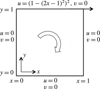
The two-dimensional lid-driven cavity configuration.

3 Application to modelling of a lid-driven cavity
The POD and sparse coding approaches are applied to model the 2-D incompressible flow in a lid-driven cavity, which is schematically depicted in figure 1. The unsteady response of a fluid enclosed in a cavity is actuated using a moving surface (lid). This configuration has been used in several studies (Leblond, Allery & Inard Reference Leblond, Allery and Inard2011; Terragni, Valero & Vega Reference Terragni, Valero and Vega2011; Balajewicz et al.
Reference Balajewicz, Dowell and Noack2013) for benchmarking purposes. The cavity considered in this study is a 2-D square enclosed region, with three rigid stationary walls and one rigid lid translating in the
 $x$
direction with constant velocity. The lid velocity is prescribed as
 $(1-(2x-1)^{2})^{2}$
, where
 $x$
varies from 0 to 1. The DNS solutions are obtained using a
 $512\times 512$
uniform grid at
 $Re$
ranging from 15 000 to 35 000, where the
 $Re$
is computed based on the maximum lid velocity. Following the case considered by Balajewicz et al. (Reference Balajewicz, Dowell and Noack2013), the modal decompositions are computed from
 $Re=30\,000$
flow data, and most of the analysis is presented for this case. The remaining flow data sets are used to study the performance of the constructed ROMs for off-design flow conditions.
The constructed ROMs are assessed in terms of the root mean square (RMS) of the flow field, and the power spectral densities of the probe velocity data, auto- and two-point covariances, and cross-power spectral densities are used to quantify comparisons between DNS, and POD and sparse ROMs. These second-order statistics are considered due to the chaotic nature of turbulent flow fields, which makes point-wise comparison an unreliable metric for assessing accuracy.
3.1 Choice of snapshot matrix
A total of 50 000 uniformly sampled observations are collected from
 $Re=30\,000$
flow over 500 units of non-dimensional time once the flow had reached a statistically stationary state. A subset of snapshots from the large set of observations is used to construct a snapshot matrix. An ‘optimal’ snapshot matrix should capture most of the important flow features while keeping the number of snapshots to a minimum. Convergence in the mean flow and instantaneous turbulent kinetic energy (
 ${\mathcal{K}}$
) quantities is used as a criterion for choosing the optimal snapshot matrix, where
 $$\begin{eqnarray}{\mathcal{K}}(t)=0.5\left(\tilde{\boldsymbol{u}}(\boldsymbol{t}),\tilde{\boldsymbol{u}}(\boldsymbol{t})\right).\end{eqnarray}$$
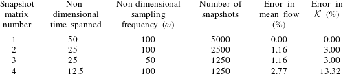
Four snapshot matrices constructed using different sampling frequencies (
 $\unicode[STIX]{x1D714}$
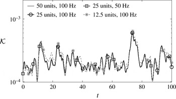
) and spanning different periods of time are considered, as summarised in table 1. The snapshot matrix numbered 1 with a sampling frequency of 100 and a time span of 50 units is used as the benchmark case, against which the rest of the three snapshot matrices are compared. Normalised L2 percentage errors in the estimated mean flow field for matrices 2, 3 and 4 are also provided in table 1. The errors in mean flow for matrices 2 and 3 are less than half of that for matrix 4. Furthermore, instantaneous
 ${\mathcal{K}}$
values are computed over 100 units of time using the mean flows obtained from each of the matrices, as shown in figure 2. The normalised L2 errors in the estimates of
 ${\mathcal{K}}$
obtained from the matrices numbered 2 and 3 are only 3 %, whereas for matrix 4 the error is as high as 13.32 %. This convergence study indicates that the first- and second-order statistics, i.e. mean flow and instantaneous
 ${\mathcal{K}}$
respectively, are converged for matrices 2 and 3. Moreover, matrix 3 contains 1250 snapshots, compared with 2500 snapshots in matrix 2. Therefore, the snapshot matrix numbered 3 with a sampling rate of 50 units and a time span of 25 units is used to construct the ROMs.
The turbulent kinetic energy (
 ${\mathcal{K}}$
) of the flow predicted by DNS over the first 100 time units, computed using the mean flow obtained from different snapshot matrices.

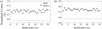
Errors in the representation of the snapshot matrix using the converged solutions for (a) 20-mode and (b) 50-mode sets. Errors for sparse modes for 30 different initial guesses are compared against POD sets of size 20 and 50.

Normalised L2 errors in estimated mean flows obtained from four different snapshot matrices, and estimated instantaneous
 ${\mathcal{K}}$
over 100 time units.

3.2 Dimensionality reduction using POD and sparse modes
The ability of the POD and sparse coding approach to carry out effective dimensionality reduction is assessed next. For this purpose, the snapshot matrix is approximated using different sets of POD and sparse modes. The normalised L2 error in the root mean square (RMS) values of the approximated fluctuating flow velocity vector is used as the performance metric. The RMS values are computed over time, at each of the grid points, for DNS and different sets of POD and sparse modes.
Mean and standard deviations of the normalised L2 errors in the representation of the RMS of the fluctuating velocity vector by 20- and 50-mode sets of sparse modes. The 20- and 50-mode POD errors are provided for reference.

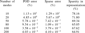
Normalised L2 errors in the representation of the RMS of the fluctuating velocity vector by POD and sparse modes, and sparsity in the representation of the snapshot matrix by sparse modes.

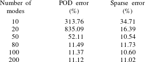
The normalised L2 error in the prediction of the RMS of the fluctuating velocity vector by several POD and sparse ROMs.

First, the sensitivity of a converged sparse coding solution to change in the initial guess for the sparse modes is studied. A set of 30 different initial guesses is used for computing 20 and 50 sparse modes. As discussed earlier, the initial guesses are obtained from randomly sampling the snapshot matrix. The RMS flow field errors in the representation of the snapshot matrix using the converged solutions for 20- and 50-sparse-mode sets are compared against those of POD sets in figure 3. The mean and standard deviation values for errors, and the difference between POD and mean sparse errors are listed in table 2. As discussed earlier, due to the optimality of POD modes in reconstructing the snapshot matrix, the POD error provides the lower bound of the global optimum of (2.7) when using the same sized sparse set. The differences between errors in the representation of the snapshot matrix using sparse modes with different initial guesses and the same number of POD modes are small. Moreover, the standard deviations in the sparse errors are significantly smaller than the mean sparse errors for both cases.
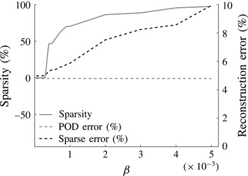
Sparsity and normalised L2 error in the representation of the snapshot matrix using sparse modes. The snapshot matrix consists of 1250 snapshots, and 20 sparse modes are computed. The 20-mode POD error is provided for reference.

The
 $u$
and
 $v$
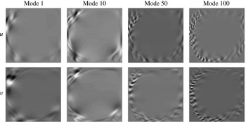
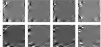
components of the POD modes numbered 1, 10, 50 and 100 of the lid-driven cavity.

Next, the normalised L2 errors in the representation of the RMS flow field by different sets of POD modes and selected sets of sparse modes of sizes 10, 20, 50, 80, 100 and 200 are compared in table 3. Again, the differences between the errors in representation using POD and sparse sets are small, with less than 1.6 % maximum difference. Additionally, the sparsity levels in the coefficient matrix output from the sparse coding process, corresponding to the different sets of sparse modes, are listed in table 3. By design, the sparsity levels lie in the range of 50–80 %.
As discussed, the sparse modes with the desired level of sparsity in the representation of the snapshot matrix are computed by varying the sparsity parameter,
 $\unicode[STIX]{x1D6FD}$
. The relationship between the
 $\unicode[STIX]{x1D6FD}$
value, the sparsity in the representation and the normalised L2 error in the reconstruction of the snapshot matrix is shown in figure 4. Here, a total of 20 sparse modes are computed, with a fixed initial guess matrix, for
 $\unicode[STIX]{x1D6FD}$
varying from
 $5\times 10^{-5}$
to
 $5\times 10^{-3}$
. The resulting sparsity increases monotonically from 0 % up to 97 %. Correspondingly, the reconstruction error increases from 4.9 % up to 10 %. It should be noted that values of
 $\unicode[STIX]{x1D6FD}$
greater than
 $5\times 10^{-3}$
failed to produce 20 sparse modes.
The
 $u$
and
 $v$
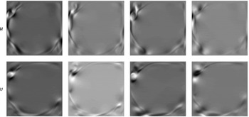
components of four of the sparse modes of the lid-driven cavity.

The
 $u$
and
 $v$
components of four different snapshots of the lid-driven cavity.

3.3 Comparison between POD and sparse modes
Comparison between POD modes, sparse modes and the original snapshots is provided next. The velocity components of the POD modes numbered 1, 10, 50 and 100, and four modes taken arbitrarily from a set of 100 sparse modes are shown in figures 5 and 6 respectively. For reference, the velocity components from the full-order solution are displayed in figure 7. The POD approach produces a set of orthogonal modes that are ordered from highest to lowest energy. Accordingly, the spatial variance of the POD modes increases with increasing mode number, where the lower-order modes capture the high-energy structures. In contrast, all of the sparse modes have mixed structures that resemble those in the flow field snapshots.
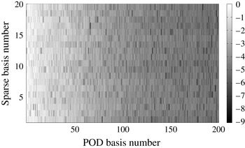
Transformation matrix between the 20 sparse modes and 200 POD modes.

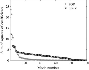
Estimated energy content in the first 100 POD modes and the sparse modes of a 100-mode model of the lid-driven cavity, expressed in terms of the sum of squares of projection coefficients evaluated over 25 time units. The estimated energy content in sparse modes is rearranged in terms of decreasing sums of squares of coefficients.

The ability of a set of sparse modes to account for the multi-scale features is studied by computing the transformation matrix between 20 sparse modes and 200 POD modes. Figure 8 shows the
 $\text{log}_{10}$
of the absolute value of the transformation matrix. A relatively large value of an element of the transformation matrix represents a higher degree of correlation between a corresponding POD mode and a sparse mode. For example, a value of 0 in figure 8 represents 100% correlation between the corresponding pair of POD and sparse modes; a value of
 $-\infty$
represents zero correlation. None of the entries are smaller than
 $-9$
. Thus, the set of 20 sparse modes contains combinations of all 200 POD modes. Consequentially, a set of sparse modes contains a broad spectrum of the large-energy and small-energy information.
The energy content in the modes is estimated as the sum of the squares of the projection coefficients corresponding to the snapshot matrix, as shown in figure 9. It should be noted that since the sparse modes are not orthogonal, the sums of squares of coefficients may overpredict the energy. Thus, this is not a precise quantitative comparison. However, it highlights the relative distribution of energy between the different sparse modes. It is observed that the energy content in the POD modes decreases rapidly with increase in mode number, with the first 17 modes accounting for approximately 90 % of the total energy. In comparison, the estimated energy distribution in the sparse modes is more uniform, or levelled.
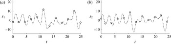
The time history of POD projection coefficients corresponding to the 100-mode POD set of the lid-driven cavity; coefficients of (a) POD mode 1 and (b) POD mode 2.

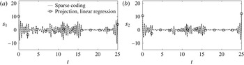
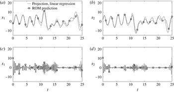
The time history of sparse projection coefficients and sparse coefficients output from the sparse coding process corresponding to the 100-mode sparse sets of the lid-driven cavity; coefficients corresponding to (a), (b) two of the sparse modes.

The RMS of the (a)
 $u$
and (b)
 $v$
velocity components of flow within the lid-driven cavity as predicted by DNS.

The RMS of the
 $u$
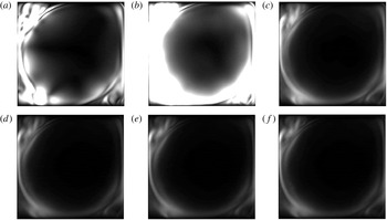
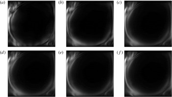
velocity component of flow within the lid-driven cavity as predicted by (a) 10-mode, (b) 20-mode, (c) 50-mode, (d) 80-mode, (e) 100-mode and (f) 200-mode POD ROMs.

The RMS of the
 $v$
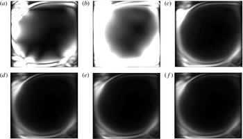
velocity component of flow within the lid-driven cavity as predicted by (a) 10-mode, (b) 20-mode, (c) 50-mode, (d) 80-mode, (e) 100-mode and (f) 200-mode POD ROMs.

The RMS of the
 $u$
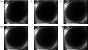
velocity component of flow within the lid-driven cavity as predicted by (a) 10-mode, (b) 20-mode, (c) 50-mode, (d) 80-mode, (e) 100-mode and (f) 200-mode sparse ROMs.

The RMS of the
 $v$
velocity component of flow within the lid-driven cavity as predicted by (a) 10-mode, (b) 20-mode, (c) 50-mode, (d) 80-mode, (e) 100-mode and (f) 200-mode sparse ROMs.

The time history of the instantaneous
 ${\mathcal{K}}$
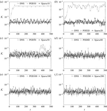
of the lid-driven cavity as predicted by DNS, and the computed POD and sparse ROMs constructed using (a) 10 modes, (b) 20 modes, (c) 50 modes, (d) 80 modes, (e) 100 modes and (f) 200 modes. The snapshot matrix used to compute the modes spans the first 25 time units, and ROMs are integrated for 500 time units.

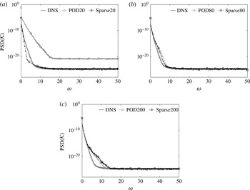
The PSD of the turbulent kinetic energy of the lid-driven cavity as predicted by DNS, and the (a) 20-mode, (b) 80-mode and (c) 200-mode POD and sparse ROMs.

The time history of projection and prediction coefficients corresponding to the 100-mode POD and 100-mode sparse sets of the lid-driven cavity; coefficients of (a) POD mode 1, (b) POD mode 2 and (c), (d) two of the sparse modes.

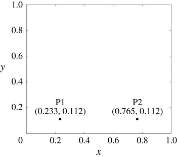
The two probe locations in the computational domain over which the local dynamics of the predicted and DNS flows are computed.

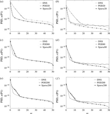
The PSDs of the
 $u$
and
 $v$
velocity components at probe P1, as predicted by DNS, POD ROMs and sparse ROMs; (a) PSD of
 $u$
by 20-mode models, (b) PSD of
 $v$
by 20-mode models, (c) PSD of
 $u$
by 80-mode models, (d) PSD of
 $v$
by 80-mode models, (e) PSD of
 $u$
by 200-mode models and (f) PSD of
 $v$
by 200-mode models.

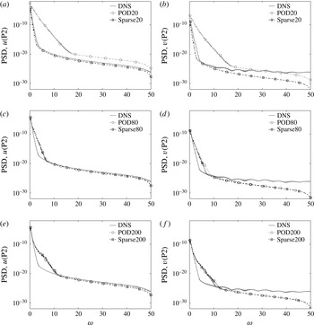
The PSDs of the
 $u$
and
 $v$
velocity components at probe P2, as predicted by DNS, POD ROMs and sparse ROMs; (a) PSD of
 $u$
by 20-mode models, (b) PSD of
 $v$
by 20-mode models, (c) PSD of
 $u$
by 80-mode models, (d) PSD of
 $v$
by 80-mode models, (e) PSD of
 $u$
by 200-mode models and (f) PSD of
 $v$
by 200-mode models.

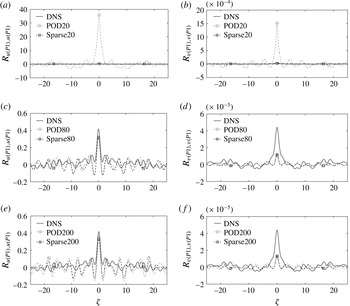
Autocovariances of the
 $u$
and
 $v$
velocity components at probe P1, as predicted by DNS, POD ROMs and sparse ROMs: (a)
 $R_{u(\text{P}1),u(\text{P}1)}$
by 20-mode models, (b)
 $R_{v(\text{P}1),v(\text{P}1)}$
by 20-mode models, (c)
 $R_{u(\text{P}1),u(\text{P}1)}$
by 80-mode models, (d)
 $R_{v(\text{P}1),v(\text{P}1)}$
by 80-mode models, (e)
 $R_{u(\text{P}1),u(\text{P}1)}$
by 200-mode models and (f)
 $R_{v(\text{P}1),v(\text{P}1)}$
by 200-mode models.

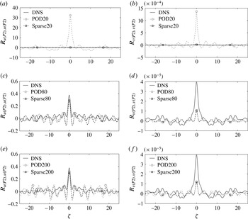
Autocovariances of the
 $u$
and
 $v$
velocity components at probe P2, as predicted by DNS, POD ROMs and sparse ROMs: (a)
 $R_{u(\text{P}2),u(\text{P}2)}$
by 20-mode models, (b)
 $R_{v(\text{P}2),v(\text{P}2)}$
by 20-mode models, (c)
 $R_{u(\text{P}2),u(\text{P}2)}$
by 80-mode models, (d)
 $R_{v(\text{P}2),v(\text{P}2)}$
by 80-mode models, (e)
 $R_{u(\text{P}2),u(\text{P}2)}$
by 200-mode models and (f)
 $R_{v(\text{P}2),v(\text{P}2)}$
by 200-mode models.

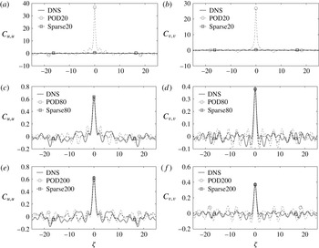
The unbiased autocovariances of the
 $u$
and
 $v$
velocity components, as predicted by DNS, POD ROMs and sparse ROMs: (a)
 $C_{u,u}$
by 20-mode models, (b)
 $C_{v,v}$
by 20-mode models, (c)
 $C_{u,u}$
by 80-mode models, (d)
 $C_{v,v}$
by 80-mode models, (e)
 $C_{u,u}$
by 200-mode models and (f)
 $C_{v,v}$
by 200-mode models.

The time varying projection coefficients of the POD modes for first 25 units of the time history are shown in figure 10. The coefficients obtained as output from the sparse coding process (Algorithm 1) are compared with projection coefficients computed using (2.9) for sparse modes in figure 11. Projections of the modes onto the snapshots using (2.9) indicate negligible activity in the time spans where the encoding of the modes to the snapshots yields zero activity. Thus, while the projection of snapshots onto the sparse modes does not yield exactly zero coefficients, the characteristically intermittent behaviour of the modal activity represents a fundamental difference with POD modes.
3.4 Predicted RMS velocity fields
The flow predictions obtained from the ROMs are compared with the full-order solutions for 500 time units. The RMS values of the flow velocities
 $u$
and
 $v$
over time, as computed using DNS, are shown in figure 12. The RMS values corresponding to the 10-, 20-, 50-, 80-, 100- and 200-mode POD and sparse ROMs are shown in figures 13–16. It should be noticed that the colour-bars used in the predicted RMS velocity flow field figures are consistent with those of DNS. The normalised L2 errors in the RMS of the fluctuating velocity vector computed over time, as predicted by POD and sparse ROMs, are listed in table 4. It is observed that the errors in predicting the RMS velocities are much smaller for the 10- to 50-mode sparse models compared with the corresponding POD models. The 10-mode sparse ROM predicts RMS flow velocities with approximately 35 % error, which is smaller than the error in prediction by the 50-mode POD model of over 50 %. Moreover, the errors converge to approximately 10–12 % for sparse models with 50 or more modes, whereas as many as 80 POD modes are required to achieve this convergence.
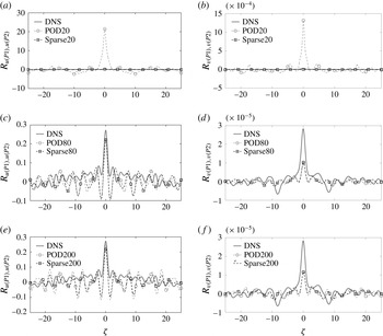
Two-point covariances of the
 $u$
and
 $v$
velocity components between probes P1 and P2, as predicted by DNS, POD ROMs and sparse ROMs: (a)
 $R_{u(\text{P}1),u(\text{P}2)}$
by 20-mode models, (b)
 $R_{v(\text{P}1),v(\text{P}2)}$
by 20-mode models, (c)
 $R_{u(\text{P}1),u(\text{P}2)}$
by 80-mode models, (d)
 $R_{v(\text{P}1),v(\text{P}2)}$
by 80-mode models, (e)
 $R_{u(\text{P}1),u(\text{P}2)}$
by 200-mode models and (f)
 $R_{v(\text{P}1),v(\text{P}2)}$
by 200-mode models.

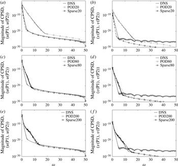
Magnitudes of the CPSDs between probes P1 and P2, as predicted by DNS, POD ROMs and sparse ROMs: CPSD of (a)
 $(u(\text{P}1),u(\text{P}2))$
by 20-mode models, (b)
 $(v(\text{P}1),v(\text{P}2))$
by 20-mode models, (c)
 $(u(\text{P}1),u(\text{P}2))$
by 80-mode models, (d)
 $(v(\text{P}1),v(\text{P}2))$
by 80-mode models, (e)
 $(u(\text{P}1),u(\text{P}2))$
by 200-mode models and (f)
 $(v(\text{P}1),v(\text{P}2))$
by 200-mode models.

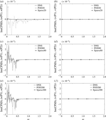
Imaginary parts of the CPSDs between probes P1 and P2, as predicted by DNS, POD ROMs and sparse ROMs: CPSD of (a)
 $(u(\text{P}1),u(\text{P}2))$
by 20-mode models, (b)
 $(v(\text{P}1),v(\text{P}2))$
by 20-mode models, (c)
 $(u(\text{P}1),u(\text{P}2))$
by 80-mode models, (d)
 $(v(\text{P}1),v(\text{P}2))$
by 80-mode models, (e)
 $(u(\text{P}1),u(\text{P}2))$
by 200-mode models and (f)
 $(v(\text{P}1),v(\text{P}2))$
by 200-mode models.

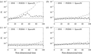
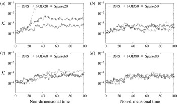
The time history of the instantaneous
 ${\mathcal{K}}$
of the lid-driven cavity at
 $Re$
15 000 as predicted by DNS, and the computed POD and sparse ROMs constructed using (a) 20 modes, (b) 50 modes, (c) 60 modes and (d) 80 modes. The POD and sparse modes are retained from the
 $Re=30\,000$
study.

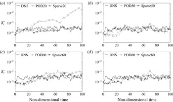
The time history of the instantaneous
 ${\mathcal{K}}$
of the lid-driven cavity at
 $Re$
29 000 as predicted by DNS, and the computed POD and sparse ROMs constructed using (a) 20 modes, (b) 50 modes, (c) 60 modes and (d) 80 modes. The POD and sparse modes are retained from the
 $Re=30\,000$
study.

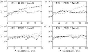
The time history of the instantaneous
 ${\mathcal{K}}$
of the lid-driven cavity at
 $Re=31\,000$
as predicted by DNS, and the computed POD and sparse ROMs constructed using (a) 20 modes, (b) 50 modes, (c) 60 modes and (d) 80 modes. The POD and sparse modes are retained from the
 $Re=30\,000$
study.

The time history of the instantaneous
 ${\mathcal{K}}$
of the lid-driven cavity at
 $Re=35\,000$
as predicted by DNS, and the computed POD and sparse ROMs constructed using (a) 20 modes, (b) 50 modes, (c) 60 modes and (d) 80 modes. The POD and sparse modes are retained from the
 $Re=30\,000$
study.

3.5 Predicted instantaneous turbulent kinetic energy
The instantaneous turbulent kinetic energy
 ${\mathcal{K}}$
predicted by ROMs is shown in figure 17. The sparse ROMs generally capture the energy levels with greater accuracy compared with the POD ROMs for the same number of modes used. When averaging over the first 500 time units, the 10- and 20-mode POD models overpredict the energy by two orders of magnitude, compared with 1.3 for the 10-mode sparse model. Similarly to the observations made for the RMS velocities, as many as 80 POD modes are required to capture the
 ${\mathcal{K}}$
levels with accuracy, whereas all of the sparse models capture the
 ${\mathcal{K}}$
levels with at least reasonable accuracy. These results are consistent with previous findings (Noack et al.
Reference Noack, Papas and Monkewitz2005; Amsallem & Farhat Reference Amsallem and Farhat2012; Holmes et al.
Reference Holmes, Lumley, Berkooz and Rowley2012; Balajewicz et al.
Reference Balajewicz, Dowell and Noack2013) that ignoring small-scale low-energy information in a truncated POD set may result in overprediction of the turbulent kinetic energy, and therefore result in an inaccurate flow prediction.
Next, the power spectral densities (PSDs) of the instantaneous turbulent kinetic energy predicted by 20-, 80- and 200-mode POD and sparse ROMs are shown in figure 18. Bendat & Piersol (Reference Bendat and Piersol2010) recommend using long time histories with integral powers of two instances for accurate PSD estimations. Therefore, the PSDs are computed over
 $2^{15}$
data points corresponding to the last 327.68 time units using Welch’s method (Welch Reference Welch1967). Furthermore, a Hanning window is used to minimise truncation errors. Consistent with the previous set of results, the 20-mode POD model significantly overpredicts the energy values over the entire range of frequencies, whereas 20-mode sparse and higher-order ROMs provide a good overall prediction.
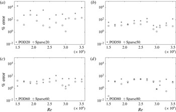
Errors in average
 ${\mathcal{K}}$
levels for POD and sparse ROMs over
 $Re$
values ranging from 15 000 to 35 000 when using (a) 20 modes, (b) 50 modes, (c) 60 modes and (d) 80 modes. The POD and sparse modes are retained from the
 $Re=30\,000$
study.

3.6 Comparison between projection and prediction coefficients
Next, the projection and prediction coefficients for the 100-mode POD and sparse models are compared in figure 19. There is good agreement between the projection and prediction coefficients for both POD and sparse ROMs over the first 10 time units, past which the prediction coefficients deviate from the projection coefficients in terms of both phase and magnitude. As noted previously, this behaviour is expected for ROMs representing chaotic full-order systems.
3.7 Predicted local flow dynamics
Next, the accuracy of POD and sparse ROMs in capturing the local dynamics of the flow within the lid-driven cavity is studied. For this purpose, the velocity data are considered at two probe locations denoted by P1 and P2, as shown in figure 20. Again, the probe data are saved for the last 327.68 time units, which correspond to
 $2^{15}$
data points.
First, the PSDs of the
 $u$
and
 $v$
velocity components computed for the two probes are shown in figures 21 and 22. The PSDs are computed following the procedure discussed in § 3.5. The 20-mode POD model overpredicts the PSD of both the
 $u$
and
 $v$
components over the first 20 units of frequency for both the probe locations, whereas the 20-mode sparse, and 80-mode and 200-mode POD and sparse models provide accurate predictions for the PSDs. It should be noticed that the PSDs are plotted in logarithmic scale, and over 99 % of the power is contained in the first three units of frequency.
Next, the autocovariances of the predicted velocities are computed for the two probe locations. The autocovariance of a random signal
 $z1(t)$
is given as (Bendat & Piersol Reference Bendat and Piersol2010)
 $$\begin{eqnarray}R_{z1,z1}(\unicode[STIX]{x1D701})=\left\langle \left(z1(t)-\unicode[STIX]{x1D707}_{z1}\right),\left(z1(t+\unicode[STIX]{x1D701})-\unicode[STIX]{x1D707}_{z1}\right)\right\rangle _{t},\end{eqnarray}$$
where
 $R_{z1,z1}$
is the autocovariance of a random signal
 $z1(t)$
,
 $\unicode[STIX]{x1D707}_{z1}$
is the mean of
 $z1(t)$
,
 $\unicode[STIX]{x1D701}$
is the non-dimensional time lag and
 $\left\langle .\right\rangle _{t}$
is the convolution operation over variable
 $t$
. The autocovariance is maximum at time lag
 $\unicode[STIX]{x1D701}=0$
, i.e. when the signal is convoluted with itself without any time lag. Moreover, the autocovariance of a random signal will sharply drop to zero as
 $|\unicode[STIX]{x1D701}|$
is increased from zero, whereas, for a constant signal, the autocovariance will acquire a constant value for all values of
 $\unicode[STIX]{x1D701}$
. Thus, the autocovariance provides a good measure of the dynamics at any given point in the flow field. The autocovariances of the
 $u$
and
 $v$
velocities at the two probe locations are provided in figures 23 and 24. The 20-mode POD model overpredicts the peak value of the autocovariance for
 $u$
by two orders of magnitude and the autocovariance for
 $v$
by an order of magnitude, whereas the 20-mode sparse, and 80-mode and 200-mode POD and sparse models capture the peak value, width of the peak and overall magnitude of the autocovariance with reasonable accuracy. Interestingly, the 20-mode sparse, and 80-mode and 200-mode POD and sparse ROMs predict the autocovariances of the
 $u$
component with better accuracy than the autocovariances of the
 $v$
component. However, it should be noticed that the magnitudes of the autocovariances of the
 $v$
component are four orders of magnitude smaller than those of the
 $u$
component. Thus, these ROMs are able to capture the overall dynamics of the flow, which corresponds to the
 $u$
component for the considered probes, with good accuracy.
The autocovariances of the flow field using an integral measure without a location bias are also considered using the following equation:
 $$\begin{eqnarray}C(\unicode[STIX]{x1D701})=\int _{\unicode[STIX]{x1D6FA}}\overline{\tilde{\boldsymbol{u}}(\boldsymbol{x},t)\boldsymbol{\cdot }\tilde{\boldsymbol{u}}(\boldsymbol{x},t-\unicode[STIX]{x1D701})}\,\text{d}x.\end{eqnarray}$$
The bias in the autocovariance (3.2) is removed by integrating the autocovariances for each of the grid points over the entire computational domain. Results for 20-, 80- and 200-mode POD and sparse ROMs are provided in figure 25. Similarly to the observations made in the previous set of results, all of the sparse and higher-order POD models provide reasonably accurate predictions for the unbiased autocovariances. However, the 20-mode POD model overpredicts the unbiased autocovariances by two orders of magnitude.
In order to further assess the capabilities of the ROMs in capturing the local dynamics, the relationships between the flow quantities at two probe locations are studied. Two-point covariances and cross-power spectral densities (CPSDs) are used for this purpose. The two-point covariance between two random signals
 $z1$
and
 $z2$
, recorded at two different probe locations, is given by (Bendat & Piersol Reference Bendat and Piersol2010)
 $$\begin{eqnarray}R_{z1,z2}(\unicode[STIX]{x1D701})=\left\langle \left(z1(t)-\unicode[STIX]{x1D707}_{z1}\right),\left(z2(t+\unicode[STIX]{x1D701})-\unicode[STIX]{x1D707}_{z2}\right)\right\rangle _{t},\end{eqnarray}$$
where
 $R_{z1,z2}$
is the two-point covariance of random signals
 $z1(t)$
and
 $z2(t)$
, and
 $\unicode[STIX]{x1D707}_{z2}$
is the mean of
 $z2(t)$
. Two-point covariance provides an estimate of the relationship between velocity signals at two probe locations. The two-point covariances between the flow quantities at two probe locations,
 $R_{u(\text{P}1),u(\text{P}2)}$
and
 $R_{v(\text{P}1),v(\text{P}2)}$
, are shown in figure 26. All of the ROMs capture the location of the peak at
 $\unicode[STIX]{x1D701}$
= 0.03 time units. However, the 20-mode POD ROM significantly overpredicts the magnitudes of the two-point covariances. Similarly to the previous observations, the 20-mode sparse, and the higher-order POD and sparse ROMs provide reasonably accurate predictions for the two-point correlations.
Next, CPSDs between the flow quantities at two probe locations are presented in figures 27 (magnitudes) and 28 (imaginary parts). The CPSD provides an estimate of the correlation between two signals in the frequency domain. The CPSDs are computed using the ‘cpsd’ function of MATLAB, which uses Welch’s method (Welch Reference Welch1967). The time domain signals are divided into seven bins with 50 % overlap between them. Additionally, a Hanning window is used to minimise truncation errors. The 20-mode sparse, and 80-mode and 200-mode ROMs capture the CPSDs over the first three frequency units accurately, whereas the 20-mode POD model overpredicts the CPSDs over the same frequency range. Moreover, the 20-mode sparse model and the higher-order ROMs capture the magnitude of the imaginary components of CPSDs with reasonable accuracy. The 20-mode POD model provides a poor prediction for the imaginary components.
3.8 Robustness of POD and sparse ROMs
The robustness of POD and sparse ROMs is assessed by computing DNS and ROM solutions with varying
 $Re$
, which for the lid-driven cavity problem here represents a change in lid velocity. However, it should be noted that the ROMs are constructed using modes extracted from a singular
 $Re$
case (30 000). The solutions are compared over 100 time units past a statistically stationary condition. The mean flows used in ROM construction are computed separately from each of the DNS simulations. The initial conditions for each of the ROMs are computed by projecting the first snapshot of the corresponding dataset onto the sets of POD and sparse modes. Representative comparisons for predicted
 ${\mathcal{K}}$
are shown in figures 29–32. The errors in time averaged
 ${\mathcal{K}}$
values for different ROMs over the range of
 $Re$
values are shown in figure 33. The 20- and 50-mode sparse models perform better than the corresponding 20- and 50-mode POD models for all of the
 $Re$
values studied. Moreover, the 20-mode POD ROM for
 $Re=31\,000$
is unstable (figure 31
a), while none of the sparse ROMs indicate any stability issues. These results suggest that sparse modes produce ROMs that are at least as robust as those generated using POD.
3.9 Computational expense
The computational costs associated with the POD and sparse ROMs computed for
 $Re=30\,000$
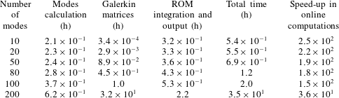
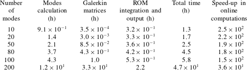
are listed in tables 5 and 6 respectively. The simulations are performed on an Intel(R) Xeon(R) E5-2620 v2 @ 2.10 GHz processor. The computation of the sparse modes is one order of magnitude more expensive than generating the POD modes. The costs to generate the Galerkin matrices and to carry out the ROM integration for POD and sparse ROMs are comparable. However, the cost of generating the Galerkin matrices is proportional to the cube of the number of modes used. This results in a high computational cost of generating a ROM when a large number of modes are used. Therefore, it is desirable to minimise the number of modes used in ROM construction, while maintaining reasonable accuracy in predictions.
Computational costs associated with several POD ROMs developed for the lid-driven cavity at
 $Re=30\,000$
. It should be noted that the modes are computed using a snapshot matrix spanning the first 25 time units, whereas the ROMs are integrated for 500 time units.

Computational costs associated with several sparse ROMs developed for the lid-driven cavity at
 $Re=30\,000$
. It should be noted that the modes are computed using a snapshot matrix spanning the first 25 time units, whereas the ROMs are integrated for 500 time units.

The speed-ups obtained in carrying out online computations are also listed in tables 5 and 6. The speed-up values are obtained by dividing the cost of CFD by the combined cost of ROM integration and output operations, where the cost for generating the 500 units of DNS data at
 $Re=30\,000$
is approximately 79.25 h. It should be noticed that the most expensive 200-mode ROMs provide a speed-up of 36. However, reasonably accurate flow predictions are obtained from 20-mode sparse ROMs with online speed-up of 250 times, whereas, when using POD modes, up to 80 modes are required to form an accurate ROM. This corresponds to an online speed-up of 180.
The sums of computational costs for several POD and sparse ROMs developed for the off-design conditions are listed in tables 7 and 8. The sum of computational costs is obtained by adding up the costs associated with ROMs developed using a fixed set of modes, over the complete range of
 $Re=15\,000$
–35 000. As the modes used for computing ROMs in the off-design conditions are retained from the
 $Re=30\,000$
case, the cost of computing modes is avoided. Moreover, the total cost of computing the high-fidelity solutions over 150 time units in all of the off-design conditions is 250.5 h, which is two orders of magnitude greater than the total ROM costs.
Sums of computational costs associated with several POD ROMs developed for the lid-driven cavity in the off-design conditions. The costs are summed over 11
 $Re$
values ranging from 15 000 to 35 000. The total cost of computing the high-fidelity solutions over 150 time units in all of the off-design conditions is 250.5 h.

Sums of computational costs associated with several sparse ROMs developed for the lid-driven cavity in the off-design conditions. The costs are summed over 11
 $Re$
values ranging from 15 000 to 35 000. The total cost of computing the high-fidelity solutions over 150 time units in all of the off-design conditions is 250.5 h.

4 Conclusions
The generation of sparse and POD modes is described with an example of a DNS database of a flow inside a 2-D lid-driven cavity. The computed POD and sparse modes are compared in terms of the energy content in the modes, the time history of the projection coefficients and the spatial structure of the
 $u$
and
 $v$
components of the modes. Several Galerkin projection based ROMs are developed. The performance of the POD and sparse ROMs is compared in terms of the evolution of the turbulent kinetic energy, the RMS of the velocities over the computational domain, the local dynamics of the predicted flow, the robustness and accuracy for varying Reynolds number, and computational expense. The results of these studies allow one to reach several useful conclusions, as follows.
-
(1) Sparse modes are inherently multi-scale, providing an a priori means to systematically incorporate both large-energy and small-energy fluid features.
-
(2) Sparse modes exhibit intermittent periods of inactivity, with only a subset of the entire set active at any instant. This property may result in modes that are more tailored to the temporally local dynamics (transience) of the system. On the contrary, the POD process yields a set of modes active at all times.
-
(3) The lower-order sparse-Galerkin ROMs significantly outperform comparable POD-Galerkin ROMs. An ROM constructed with only 20 sparse modes is found to be adequate in capturing the instantaneous turbulent kinetic energy, the RMS of velocities and the spatially local dynamics of the flow within the lid-driven cavity, whereas as many as 80 POD modes are required to obtain reasonably accurate flow predictions.
-
(4) The sparse-Galerkin ROMs are found to yield comparable robustness to POD-Galerkin ROMs for varying Reynolds number.
-
(5) The computational cost of computing sparse modes is an order of magnitude higher than the cost of computing the same number of POD modes. This increased cost is mitigated somewhat by the ability of the sparse ROMs to yield a sufficiently accurate prediction model with significantly fewer modes. Furthermore, the cost of the most expensive sparse-Galerkin models remains significantly smaller than that of solving the full-order model.
Acknowledgements
The authors gratefully acknowledge the support of ONR grant N00014-14-1-0018, under the direction of Dr J. Milgram, an HPCMPO Frontier PETTT Project Grant, under the direction of D. Bartoe, and an allocation of computing time from the Ohio Supercomputer Center. The authors thank Dr L. Agostini, Mr K. Goparaju, Mr S. Unnikrishnan and Dr D. Gaitonde, Mechanical & Aerospace Engineering, The Ohio State University for providing technical guidance in the study of local flow dynamics.