1. Introduction
The dynamics of pores in cell membranes is an important long-standing problem in the study of biological processes. When a pore forms, the cellular membrane is no longer intact and once-impermeant molecules are able to freely pass between the intra- and extracellular solution. Membrane poration of cells is experimentally replicated in giant liposomes, more or less spherical membranes tens of microns in diameter, where the formation of a pore and its growth and shrinkage can be followed in a controllable manner. The membrane of a liposome or a cell acts like a two-dimensional fluid and the interfacial forces of the membrane surface drive the changes in pore size. In this setting, inertial forces are negligible since the length scales of the flow patterns are very small and the time scales are moderate. But since both the membrane and ambient fluid are viscous and both must move, the growth or shrinkage of the pore is opposed by viscous dissipation. The viscous interaction between the ambient fluid and the movement of the membrane surface is thus central to pore dynamics.
In their classic paper, Brochard-Wyart, de Gennes & Sandre (Reference Brochard-Wyart, de Gennes and Sandre2000) derived the equation for the dynamics of a pore in a liposome,
 $$\begin{eqnarray}(C{\it\eta}_{a}{\it\varrho}+{\it\eta}_{m}){\it\varrho}^{\prime }=-{\it\gamma}+{\it\sigma}{\it\varrho},\end{eqnarray}$$
where
 ${\it\varrho}$
is the radius of the pore,
 ${\it\varrho}^{\prime }$
is the pore velocity,
 ${\it\eta}_{a}$
and
 ${\it\eta}_{m}$
are the solvent and membrane viscosities respectively,
 ${\it\gamma}$
is the edge tension and
 ${\it\sigma}$
is the membrane tension. The first term on the left-hand side arises from a scaling argument for solvent dissipation, and as such, has an undetermined coefficient
 $C$
. An assumption used in Brochard-Wyart et al. (Reference Brochard-Wyart, de Gennes and Sandre2000) is that the membrane viscosity dominates, effectively setting
 $C=0$
. With this assumption, fitting to their data yielded a value of membrane viscosity (
 ${\it\eta}_{m}$
, with dimensions of viscosity
 $\times$
length) that is approximately a hundred times greater than the actual membrane viscosity. The approximate value of membrane viscosity must be adjusted to predict the scaling of pore kinetics with solvent viscosity (
 ${\it\eta}_{a}$
), suggesting that
 $C$
cannot be zero, since both forms of viscosity should be set by their experimental value. Consequently, an accurate picture of pore dynamics involves determining this unknown coefficient.
The lifetime of a pore in a liposome generally includes three stages. First, the pore opens quickly and the membrane tension, which is the force responsible for pore enlargement, is relaxed. During this stage, some of the intracellular solution may leak out into the surrounding fluid. The second and third stages both include the closing of the pore, the former being a slow linear closure stage, and the latter a rapid closure stage. During the linear closure stage, the membrane tension builds in such a way that the opposing tensions of the pore are effectively in balance. Based on this force balance, Portet & Dimova (Reference Portet and Dimova2010) derived a formula for the dynamics of linear pore closure, and using their formula, devised a method for experimentally measuring the edge tension parameter. As observed from their data, the overall spherical shape of the membrane is conserved, and in the latter two stages, the size of the liposome is nearly constant relative to the size of the pore.
Fitting to experimental data from the final stage, the rapid pore closure stage, Ryham, Berezovik & Cohen (Reference Ryham, Berezovik and Cohen2011) determined an empirical value for the coefficient
 $C$
. They showed that lipid flow is kinetically limited by both membrane and aqueous viscosity, but for giant liposomes, solvent viscosity generally dominates over the effects of membrane viscosity. This study of pore dynamics led to the calculation of the coefficient of friction for the retraction of an infinite two-dimensional sheet with a hole, i.e. a planar bilayer with a pore surrounded by a viscous fluid. A solution to this general problem was given in Cohen & Ryham (Reference Cohen and Ryham2014). Using the solution for the two-dimensional sheet as a base, the streaming flow for a sphere was calculated perturbatively, in the regime where the radius of the pore is much smaller than the radius of the sphere.
In the present paper, we calculate an exact, closed-form streaming flow for the sphere with a pore that changes radius. The proposed solution uses a novel boundary value problem formulation for the complementary integral method (Ranger Reference Ranger1973) to develop the detailed flow field. To our knowledge, this closed form solution has not previously been reported in the literature. Following the energetic approach of Cohen & Ryham (Reference Cohen and Ryham2014), we employ the Rayleigh dissipation function (Happel & Brenner Reference Happel and Brenner1965), and use the closed-form stream function to obtain an analytical value for the coefficient
 $C$
. The result of this calculation gives realistic and excellent agreement with experimental data.
The drag coefficient depends on the shape of the bounding surface. The flow field around this shape is not known a priori and must be calculated. That is why in § 2 we formulate the precise problem to be discussed: a sphere with a pore embedded in a viscous fluid, where we calculate in closed form the stream function for a given rim velocity. In § 3 we introduce the interfacial mechanics. There we equate the energy gained per unit time with the dissipation terms as evaluated by the results from § 2. The drag coefficient
 $C$
is the shape parameter for solvent dissipation in this equation. Finally, in § 4, we examine two simplified limits: a planar membrane with a small hole and a contracting disk. In this final section we obtain results that significantly improve upon prior calculations, going beyond the classic models of pore dynamics in a number of ways. A modification of the boundary-value problem studied in this paper yields a calculation for the leak-out through a pore in a liposome. Also, the mathematically exact details supply the flow and pressure fields needed to devise numerically accurate simulations of pore dynamics in freely deformable vesicles.
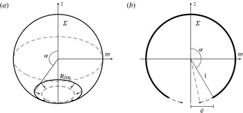
(a) Shows the spherical surface
 ${\it\Sigma}=\{r=1,0\leqslant {\it\theta}<{\it\alpha}\}$
with a pore three-dimensionally. The arrows illustrate the motion of the circular rim, which compresses or stretches surface area uniformly. (b) Depicts the two-dimensional cross-section of
 ${\it\Sigma}$
. The radius of the sphere is constant. The pore shrinks (grows) with increasing (decreasing)
 ${\it\alpha}$
: the arrows show the trajectory of the pore rim.

2. Problem formulation
We consider a sphere with a pore
 ${\it\Sigma}=\{r=1,0\leqslant {\it\theta}\leqslant {\it\alpha}\},$
embedded in a viscous fluid. The pore, the open part of the sphere
 $\{r=1,{\it\alpha}<{\it\theta}\leqslant {\rm\pi}\}$
, connects the interior and exterior fluid regions (figure 1
a);
 $(r,{\it\theta},{\it\phi})$
are spherical coordinates. In this paper we focus on changes in
 ${\it\alpha}$
governing the size of the pore and disregard the effect of leak-out (figure 1
b). Since we are considering a sphere of fixed size, we have for the radial boundary velocity
 $$\begin{eqnarray}u_{r}(1,{\it\theta})=0\quad 0\leqslant {\it\theta}\leqslant {\it\alpha}.\end{eqnarray}$$
Experimental visualization of pore expansion and closure shows no rim formation, which suggests that the surface area compresses or stretches uniformly (Sandre, Moreaux & Brochard-Wyart Reference Sandre, Moreaux and Brochard-Wyart1999; Brochard-Wyart et al. Reference Brochard-Wyart, de Gennes and Sandre2000; Karatekin et al. Reference Karatekin, Sandre, Guitouni, Borghi, Puech and Brochard-Wyart2003). Assuming this implies that the surface divergence is independent of position, and we have an equation for the tangential boundary velocity:
 $$\begin{eqnarray}\frac{\partial u_{{\it\theta}}}{\partial {\it\theta}}+\cot {\it\theta}u_{{\it\theta}}=c,\quad u_{{\it\theta}}|_{{\it\theta}=0}=0,\end{eqnarray}$$
where
 $c$
is the relative change in surface area. Integrating this equation, we obtain
 $$\begin{eqnarray}u_{{\it\theta}}(1,{\it\theta})=c\frac{1-\cos {\it\theta}}{\sin {\it\theta}},\quad 0\leqslant {\it\theta}\leqslant {\it\alpha}.\end{eqnarray}$$
Note that
 $u_{{\it\theta}}(1,0)=0$
and that
 $u_{{\it\theta}}(1,{\it\alpha})=c\tan ({\it\alpha}/2)$
. Thus
 $c=U\cot ({\it\alpha}/2)$
where
 $U$
is the tangential velocity of the pore rim. At this stage the flow is dimensionless and we pick
 $c={\rm\pi}$
for convenience. At the end of this section, we will rescale (2.3) to dimensional units.
We determine the bulk flow from the stream function formulation (Happel & Brenner Reference Happel and Brenner1965)
 $$\begin{eqnarray}u_{r}=-\frac{1}{r^{2}\sin {\it\theta}}\frac{\partial {\it\psi}}{\partial {\it\theta}},\quad u_{{\it\theta}}=\frac{1}{r\sin {\it\theta}}\frac{\partial {\it\psi}}{\partial r},\quad u_{{\it\phi}}=0.\end{eqnarray}$$
The Reynolds number for pore dynamics is small (of the order of
 $10^{-5}$
, see legend of figure 3), and so the stream function is a solution to the quasi-static Stokes system
 $$\begin{eqnarray}E^{4}{\it\psi}=0,\quad E^{2}=\frac{\partial ^{2}}{\partial r^{2}}+\frac{\sin {\it\theta}}{r^{2}}\frac{\partial }{\partial {\it\theta}}\left(\frac{1}{\sin {\it\theta}}\frac{\partial }{\partial {\it\theta}}\right),\end{eqnarray}$$
 $$\begin{eqnarray}{\it\psi}(1,{\it\theta})=0,\quad \frac{\partial {\it\psi}}{\partial r}(1,{\it\theta})={\rm\pi}(1-\cos {\it\theta})\quad 0\leqslant {\it\theta}\leqslant {\it\alpha},\end{eqnarray}$$
 $$\begin{eqnarray}{\it\psi}(r,0)={\it\psi}(r,{\rm\pi})=0,\quad 0\leqslant r<\infty ,\end{eqnarray}$$
 $$\begin{eqnarray}{\it\psi}(r,{\it\theta})=O(r),\quad r\rightarrow \infty .\end{eqnarray}$$
The boundary conditions (2.5c,d
) come from (2.1), (2.3) and (2.4) at
 $r=1$
. We look for a solution of the special form
 $$\begin{eqnarray}{\it\psi}={\textstyle \frac{1}{2}}(r^{2}-1)V,\quad E^{2}V=0,\quad V(1,{\it\theta})={\rm\pi}(1-\cos {\it\theta}),\quad 0\leqslant {\it\theta}\leqslant {\it\alpha}.\end{eqnarray}$$
The form of the solution
 ${\it\psi}$
in (2.6) follows (Dorrepaal, O’neill & Ranger Reference Dorrepaal, O’neill and Ranger1976) and is motivated by generalized axisymmetric potential theory (Weinstein Reference Weinstein1955; Payne & Pell Reference Payne and Pell1960). It can be checked by direct substitution that
 $r^{2}V$
is a solution of (2.5a
); by construction
 $V$
is also a solution. The factor
 $(r^{2}-1)/2$
enforces the Dirichlet (essential) boundary condition for
 ${\it\psi}$
in (2.5c
). The boundary condition for
 $V$
in (2.6) enforces the Neumann boundary condition for
 ${\it\psi}$
in (2.5d
).
Since
 $V$
will be determined piecewise and must be smooth away from
 ${\it\Sigma}$
, we require continuity of its normal derivative on the open portion of the sphere;
 $$\begin{eqnarray}\lim _{r\uparrow 1}\frac{\partial V}{\partial r}(r,{\it\theta})=\lim _{r\downarrow 1}\frac{\partial V}{\partial r}(r,{\it\theta}),\quad {\it\alpha}<{\it\theta}\leqslant {\rm\pi}.\end{eqnarray}$$
The function
 $V$
is irrotational and has the integral representation (Ranger Reference Ranger1973)
 $$\begin{eqnarray}\displaystyle V(r,{\it\theta}) & = & \displaystyle r^{1/2}\int _{0}^{{\it\theta}}\frac{v(r,{\it\lambda})\sin {\it\lambda}}{(\cos {\it\lambda}-\cos {\it\theta})^{1/2}}\,\text{d}{\it\lambda}=-r^{1/2}\int _{{\it\theta}}^{{\rm\pi}}\frac{w(r,{\it\lambda})\sin {\it\lambda}}{(\cos {\it\lambda}-\cos {\it\theta})^{1/2}}\,\text{d}{\it\lambda}\end{eqnarray}$$
 $$\begin{eqnarray}\displaystyle & = & \displaystyle \mathop{\sum }_{n=1}^{\infty }A_{n}r^{n+1}[P_{n-1}(\cos {\it\theta})-P_{n+1}(\cos {\it\theta})],\quad r\leqslant 1,\end{eqnarray}$$
 $$\begin{eqnarray}\displaystyle V(r,{\it\theta}) & = & \displaystyle rV(r^{-1},{\it\theta}),\quad r>1.\end{eqnarray}$$
Here,
 $P_{n}$
are Legendre polynomials of degree
 $n$
and
 $(v,w)$
are conjugate, two-dimensional harmonics:
 $$\begin{eqnarray}w(r,{\it\lambda})+\text{i}v(r,{\it\lambda})=\frac{2^{3/2}}{{\rm\pi}}\mathop{\sum }_{n=1}^{\infty }A_{n}(r\text{e}^{\text{i}{\it\lambda}})^{n+1/2}.\end{eqnarray}$$
The axial condition (2.5e
) follows from the identities
 $P_{n}(1)=1$
and
 $P_{n}(-1)=(-1)^{n}$
. From (2.6) and (2.9),
 ${\it\psi}(r,{\it\theta})\sim (3/4)A_{1}r\sin ^{2}{\it\theta}$
as
 $r\rightarrow \infty$
, yielding (2.5f
). Thus the velocities satisfy the far-field condition
 $$\begin{eqnarray}\lim _{r\rightarrow \infty }u(r,{\it\theta})=0.\end{eqnarray}$$
Consequently, the centre of the sphere is stationary relative to the far field.
To determine the values of
 $v(1,{\it\lambda})$
in the range
 $0\leqslant {\it\lambda}\leqslant {\rm\pi}$
, we set
 $r=1$
in (2.8) and compare the result with (2.6c
):
 $$\begin{eqnarray}{\rm\pi}(1-\cos {\it\theta})=\int _{0}^{{\it\theta}}\frac{v(1,{\it\lambda})\sin {\it\lambda}}{(\cos {\it\lambda}-\cos {\it\theta})^{1/2}}\,\text{d}{\it\lambda},\quad 0\leqslant {\it\theta}\leqslant {\it\alpha}.\end{eqnarray}$$
This Abel-type integral equation has the solution
 $$\begin{eqnarray}v(1,{\it\lambda})=2^{3/2}\sin \frac{{\it\lambda}}{2},\quad 0\leqslant {\it\lambda}\leqslant {\it\alpha}.\end{eqnarray}$$
From (2.7), the second equation in (2.8), and (2.10), it follows that
 $(\partial w/\partial r)(1,{\it\lambda})=0$
for
 ${\it\alpha}<{\it\lambda}\leqslant {\rm\pi}$
. From (2.11), we obtain that
 $v(1,{\it\lambda})$
is constant for
 ${\it\alpha}<{\it\lambda}\leqslant {\rm\pi}$
. Setting
 $r=1$
and
 ${\it\theta}={\rm\pi}$
in (2.8) and using (2.5e
) and (2.14) yields the value of this constant:
 $$\begin{eqnarray}\sqrt{2}v(1,{\it\lambda})=2B=(\sin {\it\alpha}-{\it\alpha})\sec \frac{{\it\alpha}}{2},\quad {\it\alpha}<{\it\lambda}\leqslant {\rm\pi}.\end{eqnarray}$$
We derive the coefficients
 $A_{n}$
from the Fourier representation of
 $v(1,{\it\lambda})$
. Setting
 $r=1$
in (2.11), taking the imaginary part and using (2.14) and (2.15) gives
 $$\begin{eqnarray}A_{n}=-\frac{\sin (n+1){\it\alpha}}{n+1}+B\frac{\cos (n+{\textstyle \frac{1}{2}}){\it\alpha}}{n+{\textstyle \frac{1}{2}}}+\frac{\sin n{\it\alpha}}{n}.\end{eqnarray}$$
These Fourier components appear in generating functions for the Legendre polynomials:
 $$\begin{eqnarray}\displaystyle & \displaystyle G({\it\zeta},x;k)=\mathop{\sum }_{n=1}^{\infty }\frac{{\it\zeta}^{n-k+2}}{n-k+2}[P_{n-1}(x)-P_{n+1}(x)]=\int _{0}^{{\it\zeta}}\frac{g({\it\xi},x)}{{\it\xi}^{k}}\,\text{d}{\it\xi}, & \displaystyle\end{eqnarray}$$
 $$\begin{eqnarray}\displaystyle & \displaystyle g({\it\zeta},x)=1+x{\it\zeta}+s^{-1}({\it\zeta}^{2}-1),\quad s=\sqrt{1-2x{\it\zeta}+{\it\zeta}^{2}}. & \displaystyle\end{eqnarray}$$
The path integral in (2.17) follows the straight line segment from 0 to
 ${\it\zeta}$
. We identify the real and imaginary parts of
 $G({\it\zeta},x;k)$
with the series resulting from the substitution of (2.16) into (2.9). The identification gives
 $$\begin{eqnarray}V(r,{\it\theta})=\text{Im}[rG({\it\zeta},x;2)-G({\it\zeta},x;1)+\text{i}Br^{1/2}G({\it\zeta},x;{\textstyle \frac{3}{2}})],\end{eqnarray}$$
where
 ${\it\zeta}=r\text{e}^{\text{i}{\it\alpha}}$
and
 $x=\cos {\it\theta}$
. To find an expression for
 $V(r,{\it\theta})$
in terms of elementary functions, we note that the functions
 $G({\it\zeta},x;k)$
admit exact integrals for
 $k=1$
,
 $k=3/2$
, and
 $k=2$
:
 $$\begin{eqnarray}\displaystyle G({\it\zeta},x;1) & = & \displaystyle x{\it\zeta}+s+x\log ({\it\zeta}-x+s)+\log (1-x{\it\zeta}+s)\nonumber\\ \displaystyle & & \displaystyle -\,1-x\log (1-x)-\log 2,\end{eqnarray}$$
 $$\begin{eqnarray}G({\it\zeta},x;{\textstyle \frac{3}{2}})=2{\it\zeta}^{-1/2}(s+{\it\zeta}x-1),\end{eqnarray}$$
 $$\begin{eqnarray}\displaystyle G({\it\zeta},x;2) & = & \displaystyle (s-1){\it\zeta}^{-1}+\log ({\it\zeta}-x+s)+x\log (1-{\it\zeta}x+s)\nonumber\\ \displaystyle & & \displaystyle +\,x-\log (1-x)-x\log 2.\end{eqnarray}$$
These yield
 $$\begin{eqnarray}\displaystyle V(r,{\it\theta}) & = & \displaystyle \text{Im}[\text{e}^{-\text{i}{\it\alpha}}(s-1)+(r-\cos {\it\theta})\log (r\text{e}^{\text{i}{\it\alpha}}-\cos {\it\theta}+s)\nonumber\\ \displaystyle & & \displaystyle +\,(r\cos {\it\theta}-1)\log (1-r\text{e}^{\text{i}{\it\alpha}}\cos {\it\theta}+s)-r\text{e}^{\text{i}{\it\alpha}}\cos {\it\theta}-s\nonumber\\ \displaystyle & & \displaystyle +\,\text{i}2B\text{e}^{-\text{i}{\it\alpha}/2}(s+r\text{e}^{\text{i}{\it\alpha}}\cos {\it\theta}-1)],\quad s=\sqrt{1-2r\text{e}^{\text{i}{\it\alpha}}\cos {\it\theta}+r^{2}\text{e}^{2\text{i}{\it\alpha}}}.\end{eqnarray}$$
Equation (2.23) defines
 $V(r,{\it\theta})$
for
 $r\leqslant 1$
,
 $0\leqslant {\it\theta}\leqslant 2{\rm\pi}$
. The inversion formula (2.10) gives the values of
 $V(r,{\it\theta})$
for
 $r>1$
. The mixed partial derivatives
 $(\partial ^{k+l}V)/(\partial r^{k}\partial {\it\theta}^{l})$
are continuous at
 $r=1$
for
 ${\it\alpha}<{\it\theta}\leqslant {\rm\pi}$
, and for all orders
 $0\leqslant l+k\leqslant 3$
. This continuity guarantees that
 ${\it\psi}(r,{\it\theta})$
given by (2.6) is smooth on the open portion of the sphere. We have numerically verified that (2.23) is a solution to the Stokes operator boundary-value problem (2.6), and that it satisfies the continuity condition (2.7) on the open portion of the sphere.
Thus the function
 $$\begin{eqnarray}{\it\psi}(r,{\it\theta})={\textstyle \frac{1}{2}}(r^{2}-1)V(r,{\it\theta})\end{eqnarray}$$
is an exact, closed-form solution of the boundary-value problem (2.5a
–
f
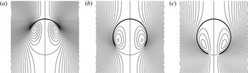
). Figure 2 depicts the streamlines of (2.24) for several values of
 ${\it\alpha}$
. For this flow, the pressure scales like
 $h^{-1/2}$
in the distance
 $h$
to the pore rim (see (A 12) in the appendix A).
The thick curves show the cross-section of
 ${\it\Sigma}$
for the angles
 ${\it\alpha}={\rm\pi}/3$
,
 $2{\rm\pi}/3$
, and
 $9{\rm\pi}/10$
(a–c). The thin curves are the flow lines calculated from (2.24). A stream surface separates the flow inside the sphere, a stagnation point lies at the base of the sphere and a stagnation ring forms inside the hole rim.

The novelty in our formulation is that the shape of the surface
 ${\it\Sigma}$
is changing, while the far field is stationary (2.12). This shows that the velocity representations devised by Ranger (Reference Ranger1973) and Dorrepaal et al. (Reference Dorrepaal, O’neill and Ranger1976) for the fixed spherical cap surface can be adapted to problems where the surface is deforming.
The preceding derivations were dimensionless. To give the problem physical dimensions, let
 $U$
be the rim velocity and
 $R$
be the radius of
 ${\it\Sigma}_{R}=\{r=R,0\leqslant {\it\theta}\leqslant {\it\alpha}\}$
. The kinematic conditions
 $$\begin{eqnarray}R{\it\alpha}^{\prime }=U=u_{{\it\theta}}(R,{\it\alpha})\end{eqnarray}$$
ensure the continuity between the fluid and rim velocity. Here
 ${\it\alpha}^{\prime }$
is the time derivative of
 ${\it\alpha}$
. Under the transformations
 $r\rightarrow r/R$
and
 $u\mapsto Uu$
, the stream function scales proportionally to
 $UR^{2}$
. From (2.4), (2.5d
) and the kinematic conditions, the proportionality constant is
 ${\rm\pi}^{-1}\cot ({\it\alpha}/2)$
. This corresponds to setting
 $c=U\cot ({\it\alpha}/2)$
in (2.3). These transformations yield the dimensional streaming flow
 $$\begin{eqnarray}{\it\Psi}(r,{\it\theta})=\frac{1}{{\rm\pi}}\cot \frac{{\it\alpha}}{2}UR^{2}{\it\psi}\left(\frac{r}{R},{\it\theta}\right).\end{eqnarray}$$
3. Aqueous drag coefficient and dissipation function
The surface
 ${\it\Sigma}_{R}$
introduced at the end of the previous section models a spherical liposome with a single pore. The radius of the liposome is
 $R$
and the radius of the pore is
 ${\it\varrho}=R\sin {\it\alpha}$
. In the classic theory of lipid pore dynamics, pore velocity
 ${\it\varrho}^{\prime }$
obeys (Brochard-Wyart et al.
Reference Brochard-Wyart, de Gennes and Sandre2000)
 $$\begin{eqnarray}(C{\it\eta}_{a}{\it\varrho}+{\it\eta}_{m}){\it\varrho}^{\prime }=-{\it\gamma}+{\it\sigma}{\it\varrho}.\end{eqnarray}$$
The membrane tension
 ${\it\sigma}$
favours pore growth while the edge tension
 ${\it\gamma}$
favours pore closure. On the left are the membrane surface viscosity
 ${\it\eta}_{m}$
and the solvent (aqueous) dissipation which scales with
 ${\it\varrho}$
and solvent viscosity
 ${\it\eta}_{a}$
. But as pointed out by Brochard-Wyart et al. (Reference Brochard-Wyart, de Gennes and Sandre2000), the scaling coefficient
 $C$
is unknown.
The surface area of
 ${\it\Sigma}_{R}$
is the apparent, microscopically observed area of the liposome. For liposomes that are microns in diameter, there exist sub-microscopic undulations (sometimes referred to as foldings or wrinkles) along the membrane of the liposome which are not represented by the smooth spherical surface. Increasing the apparent liposome area suppresses these undulations, and gives a membrane tension
 ${\it\sigma}$
with two-dimensional modulus
 $\mathscr{E}$
(Brochard, Gennes & Pfeuty Reference Brochard, Gennes and De Pfeuty1976; Brochard-Wyart et al.
Reference Brochard-Wyart, de Gennes and Sandre2000):
 $$\begin{eqnarray}4{\rm\pi}R_{0}^{2}{\it\sigma}=\mathscr{E}(4{\rm\pi}(R^{2}-R_{0}^{2})-{\rm\pi}{\it\varrho}^{2}).\end{eqnarray}$$
Here,
 $R_{0}$
is the radius of the unstretched liposome prior to pore formation. In (3.2), the area of the porated liposome is approximated by subtracting the area of a circular disk from the area of the sphere. The Laplace pressure
 $2{\it\sigma}/R$
and leak-out control liposome volume (Sampson Reference Sampson1891):
 $$\begin{eqnarray}4{\rm\pi}R^{2}R^{\prime }=-\frac{2{\it\sigma}}{3{\it\eta}_{a}R}{\it\varrho}^{3},\end{eqnarray}$$
with
 $R^{\prime }$
the time rate of change of
 $R$
. Multiplying (3.1) by
 $2{\rm\pi}$
and integrating with respect to
 ${\it\varrho},$
shows that the mechanical energy
 $W$
of the liposome is
 $$\begin{eqnarray}W={\it\gamma}2{\rm\pi}{\it\varrho}+\frac{\mathscr{E}}{2}\frac{(4{\rm\pi}(R^{2}-R_{0}^{2})-{\rm\pi}{\it\varrho}^{2})^{2}}{4{\rm\pi}R_{0}^{2}}.\end{eqnarray}$$
The membrane bending rigidity
 $K_{B}$
enters through the two-dimensional modulus
 $\mathscr{E}$
and the edge tension
 ${\it\gamma}$
(Biria, Maleki & Fried Reference Biria, Maleki and Fried2013).
In the model (3.1)–(3.3), the radius
 $R$
of the liposome is not assumed constant, as illustrated by (3.3). However, both numerical integration of (3.1)–(3.3) and experimental measurements show that
 $R$
quickly enters an effectively steady state where
 $|R^{\prime }|\ll |U|=R|{\it\alpha}^{\prime }|$
, after the pore reaches its maximum radius (Brochard-Wyart et al.
Reference Brochard-Wyart, de Gennes and Sandre2000; Karatekin et al.
Reference Karatekin, Sandre, Guitouni, Borghi, Puech and Brochard-Wyart2003; Portet & Dimova Reference Portet and Dimova2010). Thus we can calculate the value of the coefficient
 $C$
using the problem formulation (2.5a
–
f
), which assumes that
 $R$
is constant and that changes in pore radius come from changes in
 ${\it\alpha}$
. We have for the total dissipation
 ${\it\Delta}_{\mathit{total}}={\it\Delta}_{a}+{\it\Delta}_{m}$
, where
 $$\begin{eqnarray}\displaystyle & \displaystyle {\it\Delta}_{a}=\int _{\mathbb{R}^{3}}\frac{{\it\eta}_{a}}{2}|\boldsymbol{{\rm\nabla}}u+\boldsymbol{{\rm\nabla}}u^{t}|^{2}\,\text{d}x=8{\it\eta}_{a}\cot ^{2}\frac{{\it\alpha}}{2}R\left({\it\alpha}-\sin {\it\alpha}+{\it\alpha}^{2}\tan \frac{{\it\alpha}}{2}\right)U^{2}, & \displaystyle\end{eqnarray}$$
 $$\begin{eqnarray}\displaystyle & \displaystyle {\it\Delta}_{m}=2{\rm\pi}{\it\eta}_{m}U^{2}. & \displaystyle\end{eqnarray}$$
The calculations for the rate of mechanical energy dissipation in the solvent
 ${\it\Delta}_{a}$
(aqueous dissipation, see Happel & Brenner Reference Happel and Brenner1965, (2–2.4)) is found in the appendix A.1. The equation for membrane dissipation
 ${\it\Delta}_{m}$
was derived in Debrégeas, Martin & Brochard-Wyart (Reference Debrégeas, Martin and Brochard-Wyart1995) and approximates membrane dissipation for a liposome by that of a planar film (
 ${\it\alpha}\sim {\rm\pi}$
). It assumes the same surface divergence condition (2.2) used in our problem formulation (Brochard-Wyart et al.
Reference Brochard-Wyart, de Gennes and Sandre2000). The Maximum Dissipation Principle of Onsager and Rayleigh gives the balance of dissipative and conservative forces (Strutt Reference Strutt1871; Onsager Reference Onsager1931a
,Reference Onsager
b
),
 $$\begin{eqnarray}\frac{1}{2}\frac{\partial {\it\Delta}_{\mathit{total}}}{\partial U}=-\frac{1}{R}\frac{\partial W}{\partial {\it\alpha}}.\end{eqnarray}$$
The factor
 $1/2$
is consistent with the quadratic dependence in
 $U$
. The factor
 $1/R$
normalizes the variation in
 ${\it\alpha}$
(position) on the right with the variation in
 $U=R{\it\alpha}^{\prime }$
(velocity, see (2.25)) on the left. Substituting (3.4)–(3.6) in for (3.7) yields
 $$\begin{eqnarray}\displaystyle \left[\frac{4}{{\rm\pi}}{\it\eta}_{a}\cot ^{2}\frac{{\it\alpha}}{2}R\left({\it\alpha}-\sin {\it\alpha}+{\it\alpha}^{2}\tan \frac{{\it\alpha}}{2}\right)+{\it\eta}_{m}\right]U & = & \displaystyle (-{\it\gamma}+{\it\sigma}{\it\varrho})\cos {\it\alpha}\nonumber\\ \displaystyle & = & \displaystyle (C{\it\varrho}{\it\eta}_{a}+{\it\eta}_{m}){\it\varrho}^{\prime }\cos {\it\alpha}.\end{eqnarray}$$
The second equation is a restatement of (3.1). Using
 ${\it\alpha}\sim {\rm\pi}$
,
 $\cos {\it\alpha}\sim -1$
,
 ${\it\varrho}=R\sin {\it\alpha}$
and
 $U\sim -{\it\varrho}^{\prime }$
, we can eliminate terms to solve for
 $C$
. This yields
 $$\begin{eqnarray}C=\frac{4}{{\rm\pi}}\csc {\it\alpha}\cot ^{2}\frac{{\it\alpha}}{2}\left({\it\alpha}-\sin {\it\alpha}+{\it\alpha}^{2}\tan \frac{{\it\alpha}}{2}\right).\end{eqnarray}$$
From (3.5), the drag coefficient
 $C$
is defined by the relation
 $$\begin{eqnarray}2{\rm\pi}C{\it\varrho}{\it\eta}_{a}U^{2}={\it\Delta}_{a}.\end{eqnarray}$$
We compare the result in (3.9) to inexact values for the coefficient derived in earlier work. Ryham et al. (Reference Ryham, Berezovik and Cohen2011) have estimated a value
 $C\approx 8$
by curve fitting to the rapid pore closure stage in experimentally measured time courses. Setting
 ${\it\alpha}={\rm\pi}$
for the pore closure limit in (3.9) gives
 $C=2{\rm\pi}\approx 6.3$
. Thus the analytically and empirically derived values of
 $C$
are in accord. There is some experimental uncertainty in the multiple data sets used for the fitting (see Portet & Dimova Reference Portet and Dimova2010, figure 2). The numerically integrated solution curves of (3.1)–(3.3), using either the curve fit value of
 $C$
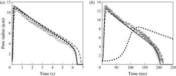
or the value derived from first principles, agree with the experimental record remarkably well (figure 3
a,b, solid and dashed curves). Importantly, the model replicates the pattern of pore dynamics using only non-adjustable physical parameters that are set by their experimental values.
Pore evolution is slowed by increasing solvent viscosity
 ${\it\eta}_{a}$
. The gray
 $\times$
are the experimental record; in (a) for (Karatekin et al.
Reference Karatekin, Sandre, Guitouni, Borghi, Puech and Brochard-Wyart2003, figure 4,
 $R_{0}=19.7~{\rm\mu}\text{m}$
,
 ${\it\gamma}=10$
pN,
 $\mathit{Re}=4.2\times 10^{-7}$
); in (b) for (Portet & Dimova Reference Portet and Dimova2010, figure 2,
 $R_{0}=20.7~{\rm\mu}\text{m}$
,
 ${\it\gamma}=14$
pN,
 $\mathit{Re}=2.0\times 10^{-5}$
). In both panels,
 $\mathscr{E}=0.046~\text{kT nm}^{-2}$
(Karatekin et al.
Reference Karatekin, Sandre, Guitouni, Borghi, Puech and Brochard-Wyart2003). Assuming
 $C=0$
(dotted curves), the numerical solution of (3.1)–(3.3) fits the experimental data in (a) provided
 ${\it\eta}_{m}=3.4\times 10^{-7}~\text{Pa}~\text{s}~\text{m}$
. But the dotted curve no longer replicates the data after setting
 ${\it\eta}_{a}$
to its value for (b). When
 $C$
is given by (3.9) and
 ${\it\eta}_{m}$
is set to the realistic value
 $3\times 10^{-9}~\text{Pa}~\text{s}~\text{m}$
, the solid curves fit the experimental data in both (a) and (b). Using the empirical value
 $C=8$
(a,b, dashed curves) yields a similar, albeit somewhat slower, time course than using the analytical value (3.9) (a,b, solid curves).

It is possible to modify the value of
 ${\it\eta}_{m}$
so that (3.1)–(3.3) fits the experimental data when ignoring the solvent dissipation. For example if
 ${\it\eta}_{a}=32~\text{mPa}~\text{s}$
, this is accomplished by setting
 $C=0$
and
 ${\it\eta}_{m}=3.4\times 10^{-7}~\text{Pa}~\text{s}~\text{m}$
(figure 3
a, dotted curve). This value of
 ${\it\eta}_{m}$
is approximately one hundred times greater than realistic membrane viscosity
 ${\it\eta}_{m}=3\times 10^{-9}~\text{Pa}~\text{s}~\text{m}$
(Dimova et al.
Reference Dimova, Aranda, Bezlyepkina, Nikolov, Riske and Lipowsky2006; Honerkamp-Smith et al.
Reference Honerkamp-Smith, Woodhouse, Kantsler and Goldstein2013; Hormel et al.
Reference Hormel, Kurihara, Brennan, Wozniak and Parthasarathy2014). Pore kinetics roughly scales with solvent viscosity
 ${\it\eta}_{a}$
, but the model (3.1)–(3.3) does not exhibit this scaling when
 $C=0$
and
 ${\it\eta}_{m}=3.4\times 10^{-7}~\text{Pa}~\text{s}~\text{m}$
(figure 3
b, dotted curve). Fitting to the experimental record for
 ${\it\eta}_{a}=1.13~\text{mPa}~\text{s}$
requires that
 ${\it\eta}_{m}$
becomes an adjustable parameter. In contrast, the term
 $C{\it\eta}_{a}{\it\varrho}$
in (3.1) obviously scales with
 ${\it\eta}_{a}$
. To illustrate that it also supplies the dissipation necessary to slow pore velocity, consider the ratio of the dissipation terms in (3.1):
 $$\begin{eqnarray}\frac{C{\it\varrho}{\it\eta}_{a}}{{\it\eta}_{m}}=\frac{C}{2}\frac{{\it\varrho}}{L_{SD}}=\frac{C\sin {\it\alpha}}{2}\frac{R}{L_{SD}}.\end{eqnarray}$$
Here
 $L_{SD}={\it\eta}_{m}/2{\it\eta}_{a}$
is the Saffman–Delbrück length (Saffman & Delbrück Reference Saffman and Delbrück1975; Brown Reference Brown2011). Assuming
 ${\it\eta}_{m}=3\times 10^{-9}~\text{Pa}~\text{s}~\text{m}$
and the viscosity of water
 ${\it\eta}_{a}=1~\text{mPa}~\text{s}$
gives
 $L_{SD}=1.5~{\rm\mu}\text{m}$
. For a characteristic liposome radius
 $R\approx 20~{\rm\mu}\text{m}$
, a pore radius
 ${\it\varrho}$
in the range 1–
 $12~{\rm\mu}\text{m}$
gives
 $2.5<{\it\alpha}<3.1$
. Using these values and (3.9), the ratio of solvent to membrane dissipation thus ranges between 2 and 20.
Equation (2.3) assumes that the velocities of the inner and outer monolayer leaflets of the membrane bilayer are the same, and consequently, intermonolayer friction is zero. Accounting for unequal change in area of the two monolayers gives a slip velocity
 ${\sim}UR^{-1}d\sin {\it\alpha}$
with the bilayer thickness
 $d$
. The intermonolayer friction resulting from this slip velocity alters the form of the membrane dissipation function
 ${\it\Delta}_{m}$
(den Otter & Shkulipa Reference den Otter and Shkulipa2007). But for liposomes microns in diameter,
 $R^{-1}d=O(10^{-3})$
and slip velocity and intermonolayer friction are negligible.
We calculated (3.9) in the regime where change in the liposome radius
 $R^{\prime }$
is small compared to the rim velocity
 $U=R{\it\alpha}^{\prime }$
. However, one may be interested in a case where
 $R^{\prime }$
and
 $U$
are comparable and
 ${\it\varrho}\sim 0$
, as occurs in the rapid pore expansion stage. In this regime, leak-out acts perpendicularly to the rim velocity (Happel & Brenner Reference Happel and Brenner1965). The rate of work done on the pore by leak-out is negligible and the rate of work done on the liposome by change in
 ${\it\alpha}$
is balanced by the lateral dissipations
 ${\it\Delta}_{a}+{\it\Delta}_{m}$
, i.e. (3.7). Thus the value for
 $C\sim 2{\rm\pi}$
in (3.9) holds in the rapid pore expansion regime as well.
Further improvements can be made to the model (3.1)–(3.3). Martínez-Balbuena, Hernández-Zapata & Santamaría-Holek (Reference Martínez-Balbuena, Hernández-Zapata and Santamaría-Holek2015) have derived a self-consistent system of equations governing the kinetics of transient pores in spherical vesicles using Onsager’s irreversible thermodynamics. But there, the dissipation function is inexact. Also, leak-out is approximated by flow through a hole in plane wall, ignoring the finite diameter and curvature of the liposome, as is the case in (3.3). Thus a complete description also requires the leak-out velocity field. Leak-out velocity satisfies a normal boundary condition, complementary to the tangential condition (2.5c,d ) used in this paper. By making an appropriate selection for the form of the stream function, an integral representation similar to (2.8) yields an exact solution for the leak-out boundary-value problem as well.
In electroporation studies, a short DC pulse significantly distorts the sphericity of the liposome. Over a short time scale, the vesicle becomes prolate or oblate ellipsoidal, or sphero-cylindrical (Riske & Dimova Reference Riske and Dimova2005; Dimova et al. Reference Dimova, Bezlyepkina, Jordö, Knorr, Riske, Staykova, Vlahovska, Yamamoto, Yang and Lipowsky2009; Salipante & Vlahovska Reference Salipante and Vlahovska2014). But pore closure occurs on a slow time scale while the liposome is nearly spherical. Thus our formulation (2.5a – f ) is applicable to electroporation on the long time scale but possibly not on the short time scale.
In appendix A.2, we show that the pressure is singular in the vicinity of the pore rim. Qualitatively, this is in agreement with the solutions of Dorrepaal et al. (Reference Dorrepaal, O’neill and Ranger1976), Cohen & Ryham (Reference Cohen and Ryham2014) and is a consequence of the assumption that the rim of the pore have zero thickness. This shows that any numerical scheme that aims to model a porated membrane by a zero thickness surface must either use mesh refinement or construct suitable local solutions to diminish the effect of pressure and stress discontinuities in the vicinity of the pore rim (Ames Reference Ames1992; Cai & Kim Reference Cai and Kim2001). Being an exact solution to the Stokes operator equation, the function (2.23) has the advantage that it supplies such a local solution and has application in the design of numerical schemes with guaranteed accuracy.
Numerical studies using the diffusive interface approach have simulated a freely deformable vesicle of finite thickness with a pore (Wang & Du Reference Wang and Du2008; Ryham, Cohen & Eisenberg Reference Ryham, Cohen and Eisenberg2012). The level set method (Salac & Miksis Reference Salac and Miksis2011) and boundary integral method (Veerapaneni et al. Reference Veerapaneni, Rahimian, Biros and Zorin2011a ,Reference Veerapaneni, Young, Vlahovska and Bławzdziewicz b ) are numerical approaches used to simulate the flow field for large deformations of intact, area-incompressible vesicles, but we are not aware of any studies that used level sets or the boundary integral method to track a vesicle with a pore.
4. Simplified limits
The closed form stream function (2.26) defines a family of flow fields for the two parameters
 $0<{\it\alpha}<{\rm\pi}$
and
 $0<R<\infty$
. As a corollary, taking limits in
 ${\it\alpha}$
and
 $R$
yields exact flows for two additional shapes; a planar membrane with a hole and a flat circular disk. Under an applied tension, the planar membrane moves radially outward, widening the hole and decreasing surface energy. A consequence of the assumption of uniform stretching and compression in the membrane surface (2.2), is that the two-dimensional divergence of the surface velocity is zero; the planar membrane is area incompressible. For this motion, we consider the cases where the dissipative forces are dominated by viscous losses in the ambient fluid. For the disk shape, surface tension drives the contraction of the circular rim. In this case, the disk is area compressible but its thickness is uniform.
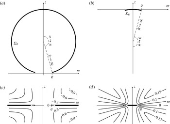
(a,c) Illustrate how
 $R$
and
 ${\it\alpha}$
are varied in the simplified limits. As
 $R$
becomes large and
 ${\it\alpha}$
approaches
 ${\rm\pi}$
,
 ${\it\Sigma}_{R}$
(a) converges to the flat membrane with a pore (c). Conversely, as
 $R$
is taken large and
 ${\it\alpha}$
approaches 0,
 ${\it\Sigma}_{R}$
(b) converges to the disk (d). (c,d) Show the surface motion under an applied tension
 ${\it\sigma}_{0}$
and the flow lines of the bulk fluid;
 $|U|$
is normalized to 1. The thick black curves depict: in (c) the membrane with a widening pore; and in (d) the disk with a contracting rim. The white arrows show the direction of rim velocity.

4.1. Planar membrane with a pore: a large sphere with a small hole
Suppose that
 $R$
and
 ${\it\alpha}$
are varied so that the diameter of the surface
 ${\it\Sigma}_{R}$
is made large and the radius of the pore
 ${\it\varrho}$
is fixed in this limit. Curvature vanishes as
 $R\rightarrow \infty$
(figure 4
a), and the shape of
 ${\it\Sigma}_{R}$
converges to that of a planar membrane with a circular hole;
 $\{{\it\varpi}>{\it\varrho},z=0\}$
(figure 4
c). Here we use cylindrical coordinates
 $({\it\varpi},z,{\it\phi})$
and oblate spheroidal coordinates
 $(p,q,{\it\phi})$
 $$\begin{eqnarray}z={\it\varrho}pq,\quad {\it\varpi}={\it\varrho}\sqrt{1-p^{2}}\sqrt{1+q^{2}},\quad 0<p<1,-\infty <q<\infty\end{eqnarray}$$
to do the calculations. We place the sphere so that the bottom pole coincides with the origin of the coordinate system
 $({\it\varpi},z,{\it\phi})=(r\sin {\it\theta},r\cos {\it\theta}+R,{\it\phi})$
(figure 4
a). That is, we take
 $z,q>0$
. For the fixed pore radius
 ${\it\varrho}=R\sin {\it\alpha}$
, we select the small, dimensionless parameter
 ${\it\epsilon}={\it\varrho}R^{-1}$
. Expanding (2.26) in a Taylor series about
 ${\it\epsilon}=0$
, we find that
 ${\it\Psi}({\it\varpi},z)={\it\psi}_{0}(p,q)+{\it\epsilon}{\it\psi}_{1}(p,q)+O({\it\epsilon}^{2})$
where
 $$\begin{eqnarray}\displaystyle & \displaystyle {\it\psi}_{0}(p,q)=U{\it\varrho}^{2}qp(p-1), & \displaystyle\end{eqnarray}$$
 $$\begin{eqnarray}\displaystyle & \displaystyle {\it\psi}_{1}(p,q)=\frac{1}{2}U{\it\varrho}^{2}\left((p-1)^{2}q^{2}+(p-1)(p^{2}-1)+\frac{pq^{2}(p^{2}-1)}{p^{2}+q^{2}}\right). & \displaystyle\end{eqnarray}$$
These terms satisfy
 $$\begin{eqnarray}\left.\begin{array}{@{}c@{}}E^{4}{\it\psi}_{0}=0,\\ {\it\psi}_{0}(0,q)=0,\\ \displaystyle \frac{\partial {\it\psi}_{0}}{\partial p}(0,q)=-U{\it\varrho}^{2}q,\\ {\it\psi}_{0}(1,q)=0,\end{array}\right\}\quad \left.\begin{array}{@{}c@{}}E^{4}{\it\psi}_{1}=0,\\ {\it\psi}_{1}(0,q)={\textstyle \frac{1}{2}}U{\it\varrho}^{2}(q^{2}+1),\\ \displaystyle \frac{\partial {\it\psi}_{1}}{\partial p}(0,q)=-U{\it\varrho}^{2}(q^{2}+1),\\ {\it\psi}_{1}(1,q)=0,\end{array}\right\}\end{eqnarray}$$
where
 $-\infty <q<\infty$
. Taking an appropriate limit of (2.26) in
 $R$
and
 ${\it\alpha}$
has led to additional solutions to Stokes equations. In order to characterize the flow fields for (4.2) and (4.3), we interpret the boundary values of (4.4). The boundary conditions for
 $p=1$
and
 $-\infty <q<\infty$
ensure that the stream function vanishes on the
 $z$
-axis, consistent with (2.5e
). The values
 $p=0$
and
 $-\infty <q<\infty$
parametrize the planar membrane with a pore of radius
 ${\it\varrho}$
. The second and third equations for
 ${\it\psi}_{0}$
in (4.4a
) give the membrane velocity
 $$\begin{eqnarray}u_{z}({\it\varpi},0)=0,\quad u_{{\it\varpi}}({\it\varpi},0)={\it\varrho}^{\prime }\frac{{\it\varrho}}{{\it\varpi}},\quad {\it\varrho}<{\it\varpi}<\infty ,\end{eqnarray}$$
where
 ${\it\varrho}^{\prime }=U$
is the velocity of the pore rim. Therefore, (4.2) describes the motion of an ambient fluid driven by a membrane with the expansion profile (4.5). Figure 4(c) depicts the flow lines for this expansion.
A consequence of the assumption used to derive (2.3) is that the surface divergence of (4.5) is zero. It models the case when the area collected by the growing pore is homogeneously spread throughout the remaining membrane. The boundary condition (2.3) thus generalizes the radial flow condition used to derive
 ${\it\Delta}_{m}$
(3.6) to the case of a sphere. The velocity profile (4.5) is observed in the bursting of free-standing viscous films under an applied tension
 ${\it\sigma}_{0}$
(Debrégeas et al.
Reference Debrégeas, Martin and Brochard-Wyart1995; Brenner & Gueyffier Reference Brenner and Gueyffier1999). Pore growth in free-standing films is limited by viscous dissipation in the film since the ambient viscosity is effectively zero (
 ${\it\varrho}{\it\eta}_{a}\ll {\it\eta}_{m}$
). These pores grow exponentially with rim velocity
 ${\it\varrho}^{\prime }={\it\sigma}_{0}{\it\varrho}/{\it\eta}_{m}$
(Debrégeas et al.
Reference Debrégeas, Martin and Brochard-Wyart1995). One application of (4.2) is that it predicts the expansion velocity when pore growth is limited by dissipation in the bulk fluid. To illustrate, consider a planar bilayer on a frame (Tien Reference Tien1974) with membrane tension
 ${\it\sigma}_{0}$
. Once the pore is large enough so that
 ${\it\gamma}\ll {\it\varrho}{\it\sigma}_{0}$
and
 ${\it\eta}_{m}\ll {\it\varrho}{\it\eta}_{a}$
, velocity is linear and satisfies
 $$\begin{eqnarray}C_{\mathit{pb}}{\it\varrho}^{\prime }=\frac{{\it\sigma}_{0}}{{\it\eta}_{a}},\quad C_{\mathit{pb}}=2{\rm\pi}.\end{eqnarray}$$
The aqueous drag coefficient
 $C_{\mathit{pb}}$
is the value of (3.9) at
 ${\it\alpha}={\rm\pi}$
. In Debrégeas et al. (Reference Debrégeas, Martin and Brochard-Wyart1995), the drag coefficient is identically 1 and characterizes internal friction of the membrane (figure 4, thick curves). Here, the drag coefficient
 $C_{\mathit{pb}}$
characterizes the internal friction of the entire solvent flow field (figure 4, flow lines).
Recently, experimentalists have measured bursting of films in viscous environments, but where motion is localized along the edge of the opening hole (Reyssat & Quéré Reference Reyssat and Quéré2006); or for a rimless film bursting parallel to the walls of a Helle-Shaw cell (Eri & Okumura Reference Eri and Okumura2010). Al-Housseiny & Stone (Reference Al-Housseiny and Stone2012) have also analysed the boundary-layer flow for a stretching sheet in laminar flow.
4.2. Contracting disk: a spherical cap with small curvature
Now we vary
 $R$
and
 ${\it\alpha}$
so that the diameter of the surface
 ${\it\Sigma}_{R}$
is fixed and
 ${\it\alpha}$
goes to zero. This produces a cap with vanishing curvature (figure 4
b). The limiting shape is a disk
 $\{{\it\varpi}<{\it\varrho},z=0\}$
(figure 4
d). To analyse this limit, we place the coordinate system
 $({\it\varpi},z,{\it\phi})=(r\sin {\it\theta},r\cos {\it\theta}-R,{\it\phi})$
at the top of the sphere, fix
 $R\sin {\it\alpha}={\it\varrho}$
and send
 $R\rightarrow \infty$
,
 ${\it\alpha}\rightarrow 0$
. Expanding (2.26) in a Taylor series for
 ${\it\epsilon}={\it\varrho}/R$
(now with
 $z,q<0$
), we find that
 ${\it\Psi}({\it\varpi},z)={\it\psi}_{0}(p,q)+O({\it\epsilon})$
where
 $$\begin{eqnarray}{\it\psi}_{0}=\frac{2}{{\rm\pi}}U{\it\varrho}^{2}pq(1-p^{2})((1+q^{2})\arg (|q|+i)-|q|).\end{eqnarray}$$
It satisfies
 $$\begin{eqnarray}\left.\begin{array}{@{}c@{}}E^{4}{\it\psi}_{0}=0,\\ {\it\psi}_{0}(p,0)=0,\\ \displaystyle \frac{\partial {\it\psi}_{0}}{\partial p}(p,0)=U{\it\varrho}^{2}p(1-p^{2}),\\ {\it\psi}_{0}(1,q)=0,\end{array}\right\}\end{eqnarray}$$
where
 $0<p<1$
and
 $-\infty <q<\infty$
. The function
 ${\it\psi}_{0}$
in (4.7) is a separable solution, but the form is less obvious than (4.2). Here the values
 $0<p<1$
and
 $q=0$
parametrize the disk with radius
 ${\it\varrho}$
. The second and third equations in (4.8) give a radial velocity that is linear in the distance to the centre of the disk:
 $$\begin{eqnarray}u_{z}({\it\varpi},0)=0,\quad u_{{\it\varpi}}({\it\varpi},0)=-{\it\varrho}^{\prime }\frac{{\it\varpi}}{{\it\varrho}},\quad 0\leqslant {\it\varpi}<{\it\varrho}.\end{eqnarray}$$
This disk is compressible (with surface divergence
 $-2{\it\varrho}^{\prime }/{\it\varrho}$
), but its thickness, if initially uniform, remains uniform. The rim velocity under an applied tension
 ${\it\sigma}_{0}$
satisfies
 $$\begin{eqnarray}C_{d}{\it\varrho}^{\prime }=-\frac{{\it\sigma}_{0}}{{\it\eta}_{a}},\quad C_{d}=\frac{32}{3{\rm\pi}},\end{eqnarray}$$
where we use
 $C=(32/3{\rm\pi})+(8/15{\rm\pi}){\it\alpha}^{2}+O({\it\alpha}^{4})$
. Moore, Saffman & Maxworthy (Reference Moore, Saffman and Maxworthy1969), Tanzosh & Stone (Reference Tanzosh and Stone1995), Davis & Stone (Reference Davis and Stone1998), and others have studied bulk fluid motion for translating, oscillating and rotating disks; (4.7) gives the bulk fluid motion generated by a contracting disk (figure 4
d). Disk entrapment and contraction dynamics has been studied experimentally and numerically by Homma, Oka & Koga (Reference Homma, Oka and Koga2011), Thoraval & Thoroddsen (Reference Thoraval and Thoroddsen2013).
Assuming
 ${\it\varrho}^{\prime }(t)$
is constant, both (4.2) and (4.7) are self-similar solutions for the unsteady Stokes equation, because
 $E^{2}{\it\psi}_{0}$
is independent of
 $t$
.
We derived (4.2)–(4.4) by making a Taylor expansion of the exact solution (2.26). Alternatively, a perturbation expansion can be applied directly to the original system (2.5a
–
f
). Matching coefficients of
 ${\it\epsilon}$
yields a system of equations which is identical to (4.2)–(4.4) (see Cohen & Ryham Reference Cohen and Ryham2014, § IV). This shows that the local boundary values for the stream function are stable under asymptotic perturbation of the domain. While the zeroth-order terms are identical, the first-order term
 ${\it\psi}_{1}$
given in (4.3) differs from the term
 ${\it\psi}^{1}$
derived by perturbation expansion (Cohen & Ryham Reference Cohen and Ryham2014, (22) and (40)). As a consequence, the velocities predicted by the exact and perturbative solutions are locally the same, but the first-order pressure and stress fields differ. The difference can be understood from the fact that in the perturbation method, one does not have the far-field boundary values for the higher-order terms in
 ${\it\epsilon}$
. In incompressible fluid flow, the pressure will change with changes in the far field, even if the local velocities are the same. Since internal pressure of a liposome is obviously consequential to membrane poration (Riske & Dimova Reference Riske and Dimova2005; Dimova et al.
Reference Dimova, Bezlyepkina, Jordö, Knorr, Riske, Staykova, Vlahovska, Yamamoto, Yang and Lipowsky2009; Salipante & Vlahovska Reference Salipante and Vlahovska2014), it is important to determine the entire flow field, not just the local flow field, as accurately as possible.
While the expansion technique is useful in many applications, it gives no sense on the size of errors (Van Dyke Reference Van Dyke1975). This makes it difficult to know whether a discrepancy (or agreement for that matter) between a perturbative calculation and experiment is caused by an unknown remainder term, the modelling assumptions or in principle both. Obtaining an exact solution is preferred since eliminating the perturbative expansion eliminates one source of uncertainty.
Acknowledgements
We thank F. S. Cohen and P. M. Vlahovska for reading an earlier draft of the manuscript, and the anonymous referees for suggesting improvements to our presentation. R.J.R. acknowledges the support of a Fordham University Faculty Fellowship and the hospitality of the Department of Molecular Biophysics and Physiology at Rush University and the Department of Engineering Sciences and Applied Mathematics at Northwestern University.
Appendix A
A.1. Calculation of the solvent dissipation function
 ${\it\Delta}_{a}$

Equation (3.5) will follow from the change of variables used to derive (2.26). We have
 $$\begin{eqnarray}\displaystyle {\it\Delta}_{a} & = & \displaystyle \int _{\mathbb{R}^{3}}\frac{{\it\eta}_{a}}{2}|\boldsymbol{{\rm\nabla}}u+\boldsymbol{{\rm\nabla}}u^{t}|^{2}\,\text{d}x=\int _{{\it\Sigma}_{R}}-\frac{{\it\eta}_{a}}{{\it\varpi}^{2}}\left[E^{2}{\it\Psi}\frac{\partial {\it\Psi}}{\partial r}\right]_{\pm }(R,{\it\theta})\,\text{d}S\nonumber\\ \displaystyle & = & \displaystyle -2{\rm\pi}{\it\eta}_{a}\left(\frac{1}{{\rm\pi}}\cot \frac{{\it\alpha}}{2}\right)^{2}U^{2}R\int _{0}^{{\it\alpha}}\frac{1}{\sin {\it\theta}}\left[E^{2}{\it\psi}\frac{\partial {\it\psi}}{\partial r}\right]_{\pm }(1,{\it\theta})\,\text{d}{\it\theta}.\end{eqnarray}$$
To arrive at (A 1), we consider separately the formulas for streaming dissipation in the two closed regions
 $\{r<R\}$
and
 $\{r>R\}$
(see Happel & Brenner Reference Happel and Brenner1965, (2–2.4) and (4–14.10)). Summing these two formulas yields overlapping surface integrals with oppositely oriented unit normals for
 $\{r=R\}$
. On the open portion of the sphere, the integrands are continuous and sum to zero. On
 ${\it\Sigma}_{R}$
, the integrands are discontinuous and their addition yields the second integral in (A 1). The prefactor
 $((1/{\rm\pi})\cot ({\it\alpha}/2))^{2}U^{2}$
is the square of the scaling constant from (2.26). The
 $R$
factor comes from the change of variables
 $r\mapsto r/R$
. The notation
 $[f]_{\pm }(a,{\it\theta})=\lim _{r\downarrow a}f(r,{\it\theta})-\lim _{r\uparrow a}f(r,{\it\theta})$
denotes the jump discontinuity.
The term
 $(\partial {\it\psi}/\partial r)(1,{\it\theta})=V(1,{\it\theta})$
in (A 1) is continuous and satisfies (2.5d
). In contrast,
 $E^{2}{\it\psi}=V+2r(\partial V/\partial r)$
is discontinuous at
 $r=1$
and so
 $[\partial V/\partial r]_{\pm }$
must be determined. We have the following identities, valid for
 $r=1$
and
 $0\leqslant {\it\theta}\leqslant 2{\rm\pi}$
:
 $$\begin{eqnarray}\displaystyle & \displaystyle s=\sqrt{1-2\text{e}^{\text{i}{\it\alpha}}\cos {\it\theta}+\text{e}^{2\text{i}{\it\alpha}}}=-\text{i}{\it\nu}\text{e}^{\text{i}{\it\alpha}/2},\quad {\it\nu}=\sqrt{2(\cos {\it\theta}-\cos {\it\alpha})}, & \displaystyle\end{eqnarray}$$
 $$\begin{eqnarray}\displaystyle & \displaystyle \frac{1-\text{e}^{\text{i}{\it\alpha}}\cos {\it\theta}+s}{\text{e}^{\text{i}{\it\alpha}}-\cos {\it\theta}+s}={\it\kappa}\text{e}^{\text{i}{\it\alpha}},\quad {\it\kappa}=\frac{{\it\nu}+2\sin {\displaystyle \frac{{\it\alpha}}{2}}}{{\it\nu}-2\sin {\displaystyle \frac{{\it\alpha}}{2}}}\quad ({\it\theta}\neq 0), & \displaystyle\end{eqnarray}$$
 $$\begin{eqnarray}\displaystyle & \displaystyle 1-\text{e}^{\text{i}{\it\alpha}}\cos {\it\theta}+s={\it\lambda}\text{e}^{\text{i}{\it\alpha}}\left({\it\nu}+2\text{i}\cos \frac{{\it\alpha}}{2}\right),\quad {\it\lambda}=\frac{1}{2}{\it\kappa}\left(2\sin \frac{{\it\alpha}}{2}-{\it\nu}\right). & \displaystyle\end{eqnarray}$$
 $r=1$
, we find that
 $$\begin{eqnarray}V(1,{\it\theta})=\left\{\begin{array}{@{}ll@{}}{\rm\pi}(1-\cos {\it\theta}), & 0\leqslant {\it\theta}\leqslant {\it\alpha},\\ \displaystyle (\cos ({\it\theta})-1)\left[2\tan ^{-1}\left(\frac{|{\it\nu}|}{2\sin {\displaystyle \frac{{\it\alpha}}{2}}}\right)-{\rm\pi}\right]-|{\it\nu}|{\it\alpha}\sec \frac{{\it\alpha}}{2}, & {\it\alpha}<{\it\theta}\leqslant {\rm\pi}.\end{array}\right.\end{eqnarray}$$
Thus
 $V(r,{\it\theta})$
obtains its boundary values (for
 $r=1,0\leqslant {\it\theta}\leqslant {\it\alpha}$
) continuously. The piecewise function (A 5) is continuous in
 ${\it\theta}$
. But for
 ${\it\alpha}<{\it\theta}\leqslant {\rm\pi}$
,
 $|{\it\nu}|=\sqrt{2(\cos {\it\alpha}-\cos {\it\theta})}$
and
 $V(1,{\it\theta})$
behaves like the square root in
 ${\it\theta}-{\it\alpha}$
. In appendix A.2, we will use the values of
 $V(1,{\it\theta})$
for
 ${\it\alpha}<{\it\theta}\leqslant {\rm\pi}$
to calculate the pressure on the open part of the sphere. Differentiating (2.19) with respect to
 $r$
and using (A 2)–(A 4), we find that
 $$\begin{eqnarray}\left.\begin{array}{@{}c@{}}\begin{array}{@{}rcl@{}}\displaystyle \frac{\partial V}{\partial r_{-}}(1,{\it\theta})\ & =\ & -{\it\nu}\cos \displaystyle \frac{{\it\alpha}}{2}-{\rm\pi}\cos {\it\theta}+2\sin \displaystyle \frac{{\it\alpha}}{2}(\sin {\it\alpha}+{\it\alpha}){\it\nu}^{-1}\\ \ & \ & +\,(\cos {\it\theta}+1)\arg \left({\it\nu}+2\text{i}\cos \displaystyle \frac{{\it\alpha}}{2}\right),\quad 0\leqslant {\it\theta}<{\it\alpha},\end{array}\\ \displaystyle \frac{\partial V}{\partial r_{+}}(1,{\it\theta})=V(1,{\it\theta})-\frac{\partial V}{\partial r_{-}}(1,{\it\theta}),\quad 0\leqslant {\it\theta}\leqslant {\rm\pi}.\end{array}\right\}\end{eqnarray}$$
The last equation follows from (2.10); it gives
 $$\begin{eqnarray}[E^{2}{\it\psi}]_{\pm }(1,{\it\theta})=2\left[\frac{\partial V}{\partial r}\right]_{\pm }(1,{\it\theta})=2V(1,{\it\theta})-4\frac{\partial V}{\partial r_{-}}(1,{\it\theta}).\end{eqnarray}$$
Substituting (2.5d ), (A 6) and (A 7) in for (A 1), we obtain a set of five integrals:
 $$\begin{eqnarray}\displaystyle {\it\Delta} & = & \displaystyle 8{\rm\pi}^{2}\int _{0}^{{\it\alpha}}\frac{1-\cos {\it\theta}}{\sin {\it\theta}}\frac{\partial V}{\partial r_{-}}(1,{\it\theta})\,\text{d}{\it\theta}-4{\rm\pi}^{3}\int _{0}^{{\it\alpha}}\frac{(1-\cos {\it\theta})^{2}}{\sin {\it\theta}}\,\text{d}{\it\theta}\nonumber\\ \displaystyle & = & \displaystyle 8{\rm\pi}^{2}\int _{0}^{{\it\alpha}}-\frac{1-\cos {\it\theta}}{\sin {\it\theta}}\left[{\it\nu}\cos \frac{{\it\alpha}}{2}+{\rm\pi}\cos {\it\theta}-2\sin \frac{{\it\alpha}}{2}(\sin {\it\alpha}+{\it\alpha}){\it\nu}^{-1}\right]\nonumber\\ \displaystyle & & \displaystyle +\,\frac{1-\cos {\it\theta}}{\sin {\it\theta}}(1+\cos {\it\theta})\arg \left({\it\nu}+2\text{i}\cos \frac{{\it\alpha}}{2}\right)-\frac{(1-\cos {\it\theta})^{2}}{2\sin {\it\theta}}\,\text{d}{\it\theta}.\end{eqnarray}$$
Performing the integrations reveals that
 $$\begin{eqnarray}{\it\Delta}=8{\rm\pi}^{2}\left({\it\alpha}-\sin {\it\alpha}+{\it\alpha}^{2}\tan \frac{{\it\alpha}}{2}\right).\end{eqnarray}$$
Substituting this expression for
 ${\it\Delta}$
into the identity
 ${\it\Delta}_{a}={\it\eta}_{a}((1/{\rm\pi})\cot ({\it\alpha}/2))^{2}U^{2}R{\it\Delta}$
gives (3.5). We remark that the formula of Payne & Pell (Reference Payne and Pell1960) cannot be used to calculate
 ${\it\Delta}_{a}$
since their formula applies to translational (rigid) motion.
A.2. Pressure in the vicinity of the pore
In spherical coordinates, the pressure
 $P$
satisfies (see Happel & Brenner Reference Happel and Brenner1965, (4–15.3) and (A-15.{1–6}))
 $$\begin{eqnarray}\frac{\partial P}{\partial r}=-\frac{{\it\eta}_{a}}{r^{2}\sin {\it\theta}}\frac{\partial }{\partial {\it\theta}}E^{2}{\it\Psi},\quad \frac{\partial P}{\partial {\it\theta}}=\frac{{\it\eta}_{a}}{\sin {\it\theta}}\frac{\partial }{\partial r}E^{2}{\it\Psi}.\end{eqnarray}$$
Using (2.26) with
 $\hat{r}=r/R$
, the fact that
 $E^{2}{\it\Psi}=(1/{\rm\pi})\cot ({\it\alpha}/2)U(V+2\hat{r}(\partial V/\partial \hat{r}))(\hat{r},{\it\theta})$
,
 $E^{2}V(\hat{r},{\it\theta})=0$
and the continuity condition
 $V=2(\partial V/\partial \hat{r})$
on the open part of the sphere (2.7), (2.10), we integrate (A 10b
) in
 ${\it\theta}$
to find
 $$\begin{eqnarray}P(R,{\it\theta})=P_{0}-\frac{{\it\eta}_{a}U}{{\rm\pi}R}\cot \frac{{\it\alpha}}{2}\left[\int _{{\it\theta}}^{{\rm\pi}}\frac{3}{2\sin {\it\theta}}V(1,{\it\lambda})\,\text{d}{\it\lambda}+\frac{2}{\sin {\it\theta}}\frac{\partial V}{\partial {\it\theta}}(1,{\it\theta})\right],\end{eqnarray}$$
for
 ${\it\alpha}<{\it\theta}\leqslant {\rm\pi}$
with the reference pressure
 $P_{0}=P(R,{\rm\pi})$
. By symmetry,
 $(\partial V/\partial {\it\theta})(1,{\rm\pi})=0$
. The integral term in (A 11) is convergent because
 $V(1,{\rm\pi})=0$
(see (2.9)); the integral is bounded independently of
 ${\it\theta}$
because
 $V(1,{\it\lambda})$
is continuous in
 ${\it\lambda}$
(see (A 5)). However, for
 ${\it\alpha}<{\it\theta}\leqslant {\rm\pi}$
, the last term
 $(\partial V/\partial {\it\theta})(1,{\it\theta})$
has a square-root singularity as
 ${\it\theta}\downarrow {\it\alpha}$
. To leading order,
 $$\begin{eqnarray}P(1,{\it\theta})\sim \frac{{\it\eta}_{a}U}{R}\frac{K}{\sqrt{\cos {\it\alpha}-\cos {\it\theta}}}\rightarrow \infty ,\quad {\it\theta}\downarrow {\it\alpha}\end{eqnarray}$$
for the positive constant
 $K=\sqrt{2}{\rm\pi}^{-1}(\sin {\it\alpha}+{\it\alpha})\csc ({\it\alpha}/2)$
. The vorticity and the strain rate tensor involve a similar square-root singularity at the pore rim.