





1. Introduction
Moving shock waves often form in industrial processes by accident or by design in cases that involve, for example, changes in combustion regimes, runaway chemical reactions or the release of high-pressure gas or combustion products (Golub et al. Reference Golub, Baklanov, Bazhenova, Bragin, Golovastov, Ivanov and Volodin2007; Duan et al. Reference Duan, Xiao, Gao, Shen, Wang and Sun2015; Cheng et al. Reference Cheng, Ji, Zhong, Long and Gao2019; Gong et al. Reference Gong, Jin, Mo, Zheng, Yao and Zhang2023). These could propagate in pipes and through various systems, causing impulsive loading that can damage valves and measuring devices. Eventually, the shock might discharge the system, propagate in open space and become a hazard to personnel in close range or cause noise disturbances at longer ranges. Hence, industrial facilities often install automatic pressure valves, passive buffers and mufflers to mitigate these risks (Jenni et al. Reference Jenni, Altorfer, Düzel, Ganz, Denzler, Tillenkamp, Zahnd and Brenner2024; Cană et al. Reference Cană, Ripeanu, Diniţă, Tănase, Portoacă and Pătîrnac2025). Transient shock-wave propagation also occurs in high-speed propulsion systems, primarily during the start-up processes of supersonic engine intakes, scramjet engines and rockets (Arad Reference Arad2024). These, typically strong shock waves, interact with the complex internal geometry of the engine, causing non-uniform loading and vibration, which might lead to immediate catastrophic damage or shorten the lifetime of the components due to localised straining. Accidental or intentional explosions can occur in underground tunnels, including the entrances to shelters, long transportation tunnels and mines (Wang et al. Reference Wang, Zhang, Wang, Li, Zhang and Zhou2021; Lin et al. Reference Lin, Hou, Derlatka, Gao, Kang and Dong2022; Gan & Remennikov Reference Gan and Remennikov2024). In addition, understanding shock propagation in non-uniform conduits is important for modelling and predicting natural processes, for example, the dynamics of explosive volcanic eruptions, in which gas jets pass through constricted vents and craters (Ogden Reference Ogden2011; Medici et al. Reference Medici, Allen and Waite2014). In these cases, internal explosions will lead to the propagation of strong shock waves in the tunnel, which typically has a non-uniform internal geometry, including structural reinforcements, transitions between sections of different cross-sectional areas, vents, splits and turns.
As a shock wave propagates in a conduit and encounters a local obstruction or constriction, it interacts with the geometry, triggering a complex, transient series of events. These include multiple shock–wall, shock–shock and shock–flow interactions. The exact morphology and subsequent evolution of these reflections, as well as the developing flow field, depend heavily on the specific obstruction geometry. The interaction of the shock wave with the obstruction initiates a transient start-up process in which the impulsively formed flow behind the incident shock wave conforms to the contour of the constriction, and the shock-wave reflections subside, reaching a steady state. Depending on the blockage ratio and the specific geometry of the narrow region, a strong shock is reflected back upstream and propagates against the incoming flow. Since a portion of the energy has been invested in the formation of the reflected shock wave, the incident shock that propagates downstream of the constriction will be weaker. As one might expect, smoother, more gradually contoured geometries create weaker reflected shock waves upstream and stronger transmitted shock downstream, and vice versa (Sloan & Nettleton Reference Sloan and Nettleton1975; Igra et al. Reference Igra, Wu, Falcovitz, Meguro, Takayama and Heilig2001; Gaetani et al. Reference Gaetani, Guardone and Persico2008; Berger et al. Reference Berger, Sadot and Ben-Dor2010).
Numerous studies have examined the interaction between shock waves and localised geometries, including abrupt changes in area, porous barriers and internal constrictions. Earlier works such as those by Monroe (Reference Monroe1959) and Dadone & Pandolfi (Reference Dadone and Pandolfi1971) examined the reflection and transmission of shock waves through orifice plates embedded in ducts, establishing early models for estimating transmitted shock strength and the onset of choking. Later efforts advanced these ideas by exploring more complicated geometries. Berger et al. (Reference Berger, Sadot and Ben-Dor2010, Reference Berger, Ben-Dor and Sadot2015) conducted systematic experimental studies of both single and multiple constrictions in a shock tube, showing that the constriction shape, blockage ratio and configuration influence the attenuation of shock loads and the resulting wave patterns. These results emphasised that, at blockage ratios of approximately 0.375, 0.5 and 0.625, geometry-induced flow features such as vortex generation and shock trapping significantly affect the pressures measured on downstream surfaces. These experimental observations have been supported by numerical studies, such as those by Rajasekar et al. (Reference Rajasekar, Yaga and Kim2023), who modelled the interaction of blast waves with barriers of varying shapes and spacings, and by Isaac et al. (Reference Isaac, Alshammari, Pickering, Clarke and Rigby2023), who summarised the effects of various types of constrictions on blast-wave loadings in urban scenarios. The propagation of a shock wave in a conduit of varying geometry and its influence on the shock has been explored through both theory and experiments for both sharp area change (Gottlieb & Igra Reference Gottlieb and Igra1983; Gichon et al. Reference Gichon, Jose, Chandravamsi, Evron and Ram2024; Kickliter et al. Reference Kickliter, Acharya and Lieuwen2025) and with varying geometries (Bird Reference Bird1959; Igra et al. 1994, 1998; Weiss et al. Reference Weiss, Grzona and Olivier2010; Dowse & Skews Reference Dowse and Skews2014; Hermet et al. Reference Hermet, Gressier and Binder2021). These studies showed that smoother contractions led to more gradual shock adaptation and reduced reflection intensity compared with sharp, step-wise area changes, which generated stronger reflected shocks and more pronounced flow separation near the contraction. These studies highlighted that the geometry of the area reduction, not just the contraction ratio, plays a crucial role in determining the strength of downstream transmitted shocks and the onset of complex flow features, such as boundary-layer detachment and vortex generation. These findings underscore the importance of considering both the curvature and the smoothness of the constriction when modelling shock–geometry interactions, as they directly affect the effectiveness of energy transmission through confined flows. In addition, they showed that a long smooth contraction significantly reduced the amplitude and duration of downstream pressure fluctuations by promoting more gradual flow adaptation.
Few studies have directly examined the effects of local constriction of the cross-section where the area contraction is followed by expansion to the same cross-section. Some information can be extracted from studies on the effects of shock interaction with porous and perforated barriers, which have been widely studied as a means to attenuate shock waves by modulating the transmitted flow through arrays of small openings. Britan et al. (Reference Britan, Igra, Ben-Dor and Shapiro2006) modelled shock interaction with orifice plates and demonstrated that the plate thickness, porosity and internal geometry of the holes significantly influence the transmitted shock strength and the generation of secondary wave structures. Ram et al. (Reference Ram, Ben-Dor and Sadot2018) showed that multiple perforated plates can create resonant cavities where shock reflections and reverberations are governed not only by porosity but also by the spacing between plates and the type of gas. Seeraj & Skews (Reference Seeraj and Skews2009) and V. et al. (Reference V., Majji, Vootla, Ram and Chandrala2024, Reference V., Majji, Anil, Ram and Chandrala2025) further found that directional porosity, achieved through staggered, angled holes, enhances impulse mitigation by dispersing the transmitted front into multiple weaker waves. While these studies focus on extended porous barriers, the physical principles underlying attenuation, namely, rapid area changes, flow choking and shock diffraction through confined openings, are closely related to those present in a localised geometric constriction. Recent experimental studies (Langdon et al. Reference Langdon, Nurick and Du Plessis2011; Schunck & Eckenfels Reference Schunck and Eckenfels2021) and numerical simulations (Kumar et al. Reference Kumar, Reddy, Sai and Kumar2017) also highlight the analogy that when a shock interacts with a porous medium, each pore behaves as a localised nozzle or contraction. The resulting flow features, such as shock focusing, vortex shedding and boundary-layer separation within the pore, mirror the interactions observed when a shock passes through a short constriction in a duct. In all cases, the blockage ratio, length scale and internal curvature of the flow path play critical roles in determining the ratio between transmitted and reflected shock strength and in governing the downstream impulsive flow field. Thus, although porous barriers and duct contractions differ in global geometry, their underlying physics is fundamentally similar, making studies of one highly relevant to understanding the other.
Taken together, existing studies provide a solid foundation for understanding how the blockage ratio and contraction shape influence the multiscale shock–wall, shock–shock and shock–flow interactions that arise when a moving shock propagates through a constriction section of a straight conduit. These works have established key trends in reflected and transmitted shock strengths and have clarified the role of abrupt versus gradual area changes in shaping the global wave dynamics. The qualitative tendencies are, by now, well established: stronger blockage produces a stronger reflected and a weaker transmitted shock, and smoother, longer contractions weaken the upstream reflection. Nevertheless, several aspects of the problem remain only partially resolved, motivating the present study. In particular, most available investigations explore a restricted subset of geometric parameters, typically varying either the blockage ratio, the contraction length or an overall area change while holding other degrees of freedom fixed. As a result, the coupled influence of these parameters on the redistribution of energy between reflected and transmitted waves, as well as on the structure of the impulsively generated downstream flow, has not been systematically characterised. A unified view of how blockage and length act together to shape the transient shock system is therefore still lacking. Moreover, prior work has largely focused on canonical geometries such as sharp orifices, steps or single, idealised nozzle contours. While these configurations have yielded valuable physical insight, they do not span the broader class of smoothly contoured constrictions in which curvature and surface smoothness can significantly alter the transient build-up of the reflected shock system, the approach to choking, and the emergence of jetting and secondary shock structures. Finally, the start-up process itself, defined as the short-time, highly unsteady adjustment from the passage of an incident planar shock to a quasi-established flow configuration, has received comparatively limited attention. Open questions remain regarding the temporal sequence, sensitivity and geometric dependence of key flow features, including separation regions, shear-layer formation and the establishment of standing shocks within the throat. Addressing these gaps requires experiments and analysis that resolve both the geometric parameter space and the early-time transient dynamics, which is the focus of the present study.
In this study, we address this gap by systematically varying both the blockage ratio and the axial length of a smooth, localised constriction and comparing it with an abrupt-step constriction. We resolve the shock-wave interaction with the constriction and the subsequent start-up dynamics using high-order implicit large-eddy simulation (LES), which are validated against time-resolved schlieren and wall-pressure measurements. We (i) quantify how the coupled
 $h/H,\,L/H$
parameters control the rate at which the reflected system develops and the ultimate balance between reflected and transmitted shocks; (ii) identify geometry-dependent pathways for secondary structure formation of standing shocks, expansion fans, shear-layer separation and jetting in the throat and their signatures in pressure histories; (iii) propose reduced-order models for predicting the late-time transmitted and reflected shock-wave strengths; and (iv) develop a reflection-corrected geometrical shock-dynamics framework that predicts the transmitted shock strength.
2. Problem description
Schematic figure of the problem; (a) represents the initial condition for a rectangular constriction and (b) represents the later state. (c,d) Represent the same for a sinusoidal constriction. Here,
 $H$
is the conduit height,
 $h$
is the constriction height,
 $L$
is the constriction length,
 $p$
is pressure,
 $T$
is temperature,
 $\rho$
is density and
 $u$
is particle velocity.

Figure 1 illustrates the configurations investigated in this study. In the first configuration, the shock wave interacts with an abrupt, rectangular, localised constriction of the conduit, as shown in figures 1(a) and 1(b). The second configuration considers a smooth, localised constriction, enabling a direct comparison between sharp and gradually contoured sinusoidal geometries, as in figures 1(c) and 1(d). The geometries are two-dimensional, featuring a symmetric converging–diverging section with a uniform conduit height,
 $H$
, on either side of the constriction. Both geometries permit variation in blockage ratio and length. The rectangular obstacle introduces sharp leading and trailing edges, whereas the sinusoidal contour imposes gradual curvature changes that influence boundary-layer separation. The use of these two configurations allows us to systematically examine how the constriction height,
 $h$
, and length,
 $L$
, govern the strength and structure of both the reflected and transmitted shock waves, as well as the evolution of the impulsively driven flow field within the constriction. Both geometries are fully defined by these two parameters, thereby limiting geometric variability while still enabling independent control of the blockage ratio,
 $\textrm{BR} = 2h/H$
, and the normalised length,
 $\tilde {L} = L/H$
. For clarity, all normalised quantities are denoted by
 $\tilde {\boldsymbol{\cdot }}$
; unless otherwise specified, lengths are normalised by the conduit height
 $H$
and pressures by the ambient pressure
 $P_0$
.
In the studied scenario, a normal shock wave with a moderate incident Mach number,
 $M_I$
, of
 $1.4$
and
 $1.8$
propagates through initially quiescent atmospheric air (marked as state 0) and produces an abrupt jump in pressure, density, temperature and velocity, to state 1 immediately behind the incident shock. Upon reaching the localised constriction, the shock wave interacts with the geometry and splits into a reflected shock that propagates upstream with a Mach number
 $M_R$
, and a transmitted shock that continues downstream with a Mach number
 $M_T$
. The reflected shock further compresses the flow behind the incident shock, generating state 2. Downstream of the constriction, the transmitted shock expands and, after some distance, resumes a normal, uniform propagation that is weaker than the incident shock due to energy partitioning and geometric effects, forming state 3.
The sinusoidal contour of the constriction used in this study is
 \begin{align} f(x)=\frac {h}{2}\left (1+\sin \left (\frac {2\pi x}{L}-\frac {\pi }{2}\right )\right ) \quad \text{for}\quad 0\leqslant x\leqslant L. \end{align}
This geometry has been chosen since it provides a smooth transition from the straight conduit into the constriction. Hence, this geometry isolates the geometric effects on shock propagation through the constriction without introducing the complexity of a sharp discontinuity along the shock path. The smooth transition prevents spurious reflections that do not arise from the constriction itself and would otherwise obscure the results. While the rectangular geometry always provides a straight-angle wall section facing the incident shock, the maximum slope of the sinusoidal geometry varies with different blockage and length ratios. It can be calculated by taking the derivative of the profile at
 $L/4$
, resulting in a maximum slope of
 $\pi h/L$
, and maximum angle
 $\theta _{\textit{max}} = \tan ^{-1}\! (\pi h/L )$
.
All of the cases examined in this study used a square tunnel with
 $H$
= 40 mm. The test matrix for the geometries examined in this study is summarised in table 1, which lists the blockage ratio,
 $h/L$
, and the maximum surface-slope angle at
 $L/4$
. The minimum blockage ratio used in this study is 0.35, corresponding to
 $\tilde {h}=0.175$
(
 $h=7\text{mm}$
), which is above the minimum blockage required to achieve choked flow in the constriction. This has been calculated for the sinusoidal geometry, assuming isentropic flow in the upstream section of the contraction at late times. Appendix B presents the calculation showing that, under these assumptions, the flow becomes choked when
 $\tilde {h}$
= 0.15 (
 $h\sim$
= 6 mm), and a numerical simulation of the local Mach number along the centreline of the constriction at different times after shock-wave impingement, validating that for
 $\tilde {h}$
= 0.125 (
 $h$
= 5 mm) the flow is not choked, but for
 $\tilde {h}$
= 0.15, it is.
Geometric parameters of the constriction section for the three constriction lengths considered.

Table 1. Long description
A table comparing geometric parameters for different constriction lengths. The table has 4 rows and 10 columns. Column headers are h-tilde, BR, L-tilde = 0.25 h/L, theta_max (degrees), L-tilde = 1 h/L, theta_max (degrees), L-tilde = 2 h/L, theta_max (degrees). Row 1: h-tilde 0.175, BR 0.35, h/L 0.70, theta_max 65.5, h/L 0.175, theta_max 28.8, h/L 0.0875, theta_max 15.4. Row 2: h-tilde 0.25, BR 0.50, h/L 1.00, theta_max 72.0, h/L 0.25, theta_max 38.0, h/L 0.125, theta_max 21.4. Row 3: h-tilde 0.30, BR 0.60, h/L 1.20, theta_max 75.0, h/L 0.30, theta_max 43.0, h/L 0.15, theta_max 25.0. Row 4: h-tilde 0.375, BR 0.75, h/L 1.50, theta_max 78.0, h/L 0.375, theta_max 49.7, h/L 0.1875, theta_max 30.5.
Rectangular models with similar geometric features were also considered; however, for all such cases the interaction angle was fixed at
 $90^\circ$
on both sides.
All quantities are normalised by the conduit height
 $H = 40$
mm.
When a shock wave encounters a localised constriction, it induces a complex sequence of wave interactions and unsteady flow phenomena, including shock reflection at the entrance to the constriction, shock focusing or standing shock formation within the throat and trailing expansion waves. The precise nature and intensity of these features depend not only on the incoming shock Mach number but also on the shape and extent of the constriction. While short constrictions act as abrupt obstructions, promoting strong initial reflections and jet-like flow downstream, longer transitions allow the flow to adapt more gradually, producing weaker reflections but generating complex shock structures inside the narrowed region. The blockage ratio strongly influences the strength of the upstream reflection and of the transmitted shock.
To isolate the effects of length and blockage ratio, we perform a series of controlled numerical simulations using a high-order compressible Navier–Stokes solver with LES modelling (Chandravamsi et al. Reference Chandravamsi, Chamarthi, Hoffmann and Frankel2023; Chandravamsi & Frankel Reference Chandravamsi and Frankel2024). The simulated flow field is validated against experimental observations using time-resolved schlieren imaging from the shock-tube facility. Our goal is to develop a mechanistic understanding of how geometry governs the partitioning of wave energy between reflected and transmitted fronts and to lay the groundwork for a predictive framework linking shock properties and conduit design to wave attenuation and downstream loading.
The analysis presented in the next sections is structured to first resolve the short-time start-up processes that occur immediately after the impingement of the incident shock on the constriction, and then examine how this transient dynamics relates to the stabilised reflected and transmitted shock waves propagation at later times. We begin by investigating the transient response within and near the constriction using time-resolved flow visualisations and centreline pressure distributions, allowing us to identify the reflection mechanisms, wave interactions and internal flow adjustments that govern the early redistribution of compression across the constriction. Once these processes subside and the flow approaches a quasi-steady configuration, the reflected and transmitted shocks propagate away from the constriction with well-defined strengths and structures that can be systematically related to blockage ratio and constriction length. The results are presented by comparing the rectangular and sinusoidal cases, which represent two extreme cases of shock–structure interaction.
3. Methods
3.1. Large-eddy simulations
This study is primarily based on numerical data obtained from our in-house LES solver for the three-dimensional compressible Navier–Stokes equations that uses a conservative low-dispersion finite-difference framework. The solver has previously demonstrated accuracy in resolving shock-wave propagation in conduits with abrupt area variation (Gichon et al. Reference Gichon, Jose, Chandravamsi, Evron and Ram2024). Inviscid fluxes are computed using the sixth-order optimised upwind reconstruction scheme of Chandravamsi et al. (Reference Chandravamsi, Chamarthi, Hoffmann and Frankel2023), combined with the monotonicity-preserving limiter of Suresh & Huynh (Reference Suresh and Huynh1997) for shock capturing. Conservative fluxes are obtained using the Harten–Lax–van Leer–contact approximate Riemann solver (Harten et al. Reference Harten, Lax and van Leer1983; Toro Reference Toro1997). Viscous fluxes are discretised using the sixth-order midpoint-based explicit optimised scheme proposed by Chandravamsi & Frankel (Reference Chandravamsi and Frankel2024). The scheme provides low dispersion and controlled damping at high wavenumbers, which suppresses odd–even decoupling while preserving the dynamically relevant scales. Time integration is performed using the third-order total-variation-diminishing Runge–Kutta scheme of Gottlieb & Shu (Reference Gottlieb and Shu1998). Subgrid-scale effects are represented implicitly through the intrinsic numerical dissipation at high wavenumbers, consistent with the implicit LES paradigm (Ahn et al. Reference Ahn, Lee and Mihaescu2021; Chandravamsi et al. Reference Chandravamsi, Chamarthi, Hoffmann and Frankel2023). The solver is formulated in curvilinear coordinates with multi-block grids to accommodate complex geometries and has been extensively validated for a broad class of compressible flows (Chandravamsi et al. Reference Chandravamsi, Chamarthi, Hoffmann and Frankel2023; Kakumani et al. Reference Kakumani, Chamarthi, Hoffmann and Frankel2023). Temperature-dependent viscosity is modelled using Sutherland’s law (Sutherland Reference Sutherland1893).
The geometry and initial conditions of the problem were chosen based on the experimental set-up. The computational domain includes only the driven and test sections, excluding the driver sections. Following a grid convergence test (see Appendix A), all the simulations were performed under a grid resolution of 30 million cells. Grid clustering was employed near the wall and the entrance region of the test section with
 $x_{\textit{min}} = y_{\textit{min}} = 110 \rm \,\mu m$
to capture the fine scales. Although the grid resolution employed is not fully sufficient to capture all the turbulent scales, the purpose of the present numerical simulations was restricted to accurately capturing the shock structure evolution and its downstream propagation. All the walls in the computational domain are imposed with the adiabatic wall boundary condition. At the entrance and exit of the geometry, characteristic non-reflecting boundary conditions (Poinsot & Lelef Reference Poinsot and Lelef1992) are employed to ensure no reflections enter the duct.
3.2. Experimental system
Schematics of the experimental system; (a) the shock-tube apparatus, (b) the interchangeable constriction model installed in the test section and (c) the optical set-up used to perform high-speed schlieren imaging.

Figure 2. Long description
Panel A: A schematic of the shock-tube apparatus. The apparatus consists of a 3-meter driver section, a 4-meter driven section, a test section, and a fast opening valve separating the driver and driven sections. The test section is enclosed in a frame, and the entire setup is aligned horizontally. Panel B: A detailed view of the interchangeable constriction model installed in the test section. The model features a flow path with pressure transducers positioned along the sides. The model is designed with interchangeable sections, each measuring 40 millimeters in width and height. Panel C: A diagram of the optical setup used for high-speed schlieren imaging. The setup includes parabolic mirrors, a high-speed camera with an iris and lens, and an LED light source with an iris and lens. Flat mirrors are used to direct the light path through the test section to the high-speed camera.
Experiments are conducted in the Transient Fluid Mechanics Laboratory shock tube at the Technion – Israel Institute of Technology. Figure 2(a) depicts the shock-tube apparatus designed with a
 $3000\,\mathrm{mm}$
long,
 $52.5\,\mathrm{mm}$
inner diameter driver section and a
 $4080$
mm long,
 $40 \times 40$
mm
 $^2$
cross-section driven section. These dimensions allow us to perform experiments with constant inlet properties to the test section for 3–6 ms, depending on the Mach number.
The shock tube is connected to a square test section that is
 $1000\,\mathrm{mm}$
long and
 $40\,\mathrm{mm}$
wide, fitted with an interchangeable, symmetric blockage insert. A partial model of the test section is shown in figure 2(b). The models were made from rigid plastic and held in place via a dovetail groove machined into the aluminium wall of the test section, ensuring minimal reflections along the connecting line. This modular section enables systematic measurements of shock propagation through a localised constriction with controllable geometry, blockage ratio and streamwise length. The test section is fitted with two 40 mm thick clear acrylic windows that enable unobstructed optical access to record the flow field and shock waves’ evolution. Pressure is recorded in the shock tube from 8 flush-mounted transducers (Endevco 8530B-500 and 136 signal conditioners) using four oscilloscopes (LeCroy 3034Z) at 250 kHz. Two transducers are located 1000 mm apart upstream of the test section entrance to calculate the inlet incident shock-wave Mach number. The imaging and the data acquisition systems are synchronised using an external timing box (Quantum composers 9400) triggered by the shock-wave arrival at the first pressure transducer mounted before the test section. High-speed schlieren imaging is used to validate the numerical data.
A schematic description of shock-wave interaction with a local constriction in a straight conduit. (a–d) Depict the interaction with a smooth sinusoidal local constriction. (e–h) Depict the interaction with a sharp rectangular local constriction. Here, RS – reflected shock wave, TS – transmitted shock wave, SS – standing shock wave.

A schematic of the schlieren set-up is presented in figure 2(c). An LED light (Thorlabs CWHL5-C1) is directed through a pinhole to reduce non-uniformity in the beam and collimated using a parabolic mirror (Edmund Optics # 32-276-533) with an unobstructed diameter of 286 mm. The collimated beam is aligned using two flat optical mirrors so that the light propagates perpendicularly through the test section. The collimated beam is focused using a similar second parabolic mirror through an iris at its focal point. The iris opening is set to create a schlieren image sensitive enough to capture the density variations in the flow that form downstream of the constriction. An imaging lens is used to form the image of the test section at the plane of the camera sensor (Phantom V2640), enabling recording of the flow field at up to 80 kHz with a resolution of 1024
 $\times$
256 pixels. The air in the driven and test sections was kept at atmospheric conditions before the experiments, as the end of the shock tube remained open. We have allowed for a long time (approximately 10 minutes) between experiments for the condition in the driven and test sections to re-equalise with the laboratory air. Consecutive experiments are run with a sufficient delay to ensure that the incident shock wave propagates into quiescent air with uniform atmospheric properties. The experiments are performed without an end wall to prevent the return of a reflected shock from the end of the test section, thereby extending the duration of the experiment.
4. Results
4.1. The main features of shock-wave interaction with local constriction
This study compares various local constriction geometries and their effects on flow and shock-wave evolution. The following description outlines the main features observed in our analysis of shock propagation, which are discussed in further detail in the next sections. A schematic description of the transient evolution of the interaction between a shock wave and a local constriction in a conduit is presented in figure 3 for both a smooth constriction (a–d) and for a sharp rectangular constriction (e–h). First, as the incident shock moves into the quiescent air and reaches the constriction at a uniform velocity
 $M_I$
, it impinges on the constriction. Immediately, the shock forms reflections at the walls, depending on the geometry. In the smooth case (figure 3
a), the reflection always begins as a weak Mach reflection (MR), and as the surface elevation increases, the reflection becomes stronger until reaching the maximum angle at
 $L/4$
. The maximum slope angle depends on the specific
 $L$
and
 $h$
of the model, as shown in table 1. For geometries in which the angle becomes sufficiently large, the reflection will transition to a regular reflection (RR). The transition occurs at an angle that depends on the Mach numbers, which can be calculated for the quasi-steady case (Ben-Dor Reference Ben-Dor2007), but, for the transient case, they differ significantly, with reports placing the transition angle for moderate Mach numbers of 1.2–1.8 at 52
 $^\circ$
to 60
 $^\circ$
(Ben-Dor Reference Ben-Dor2007; Geva et al. Reference Geva, Ram and Sadot2013). In this study we performed analysis for
 $M_I =$
1.4 and 1.8. To allow direct comparison between cases, only
 $M_I=1.4$
is presented in the figures. The results for
 $M_I=1.8$
exhibit similar trends to those of
 $M_I=1.4$
. Reflected and transmitted shock-wave speeds for
 $M_I=1.8$
are given in figures 13 and 14. In the rectangular-geometry case, figure 3(e), when the shock impinges head-on on the flat 90
 $^\circ$
face of the model, the reflected shock forms immediately, and a MR forms between the incident shock and the shock that propagates in the narrow region. In this case, the induced flow behind the shock wave interacts with the sharp upstream-facing corner, leading to immediate flow separation into a growing vortex. We have found that, in the sinusoidal, smooth geometry, the separation of flow begins in later stages, as further discussed in § 4.3. The shock waves that are reflected upstream expand, forming a reflected shock propagating upstream against the flow induced by the incident shock wave.
As the shock passes through the throat of the constriction, it begins to expand, forming a curved expanding transmitted shock. In the case of the sinusoidal geometry (figure 3
b), as long as the shock wave is moving along the surface of the expanding region, it does not form a reflection. However, when the surface angle begins to decrease (i.e. downstream of
 $3L/4$
), a MR forms, which persists as the transmitted shock propagates downstream. In the rectangular constriction case, the transmitted shock wave expands along the vertical walls of the downstream expansion and impinges head-on onto the walls of the conduit, as depicted in figure 3( f). Since the angle between the transmitted expanding shock wave and the wall is small, a RR will form initially. Further downstream, the transmitted shock curvature will decrease, increasing the angle between the shock wave and the wall until the shock also transitions to a MR. A full description of this process is presented in Gichon et al. (Reference Gichon, Jose, Chandravamsi, Evron and Ram2024).
As the two primary shock waves, i.e. the transmitted and reflected shocks, continue to propagate away from the constrictions, the MRs will evolve so that the triple point will reverberate between the two walls of the conduit, forming multiple reflections behind them. In essence, the reflection pattern of the transmitted and reflected shock will become quite similar from this point on, as depicted in figures 3(c) and 3(g). Naturally, as the shock waves propagate away from the constriction, the repeated reflections behind them will subside, and the shock fronts will resume their normal, uniform state. The transmitted and reflected shocks will depend on the geometry and will be discussed in detail throughout the following sections. The geometry of the constriction will strongly affect the transient start-up processes within it as the primary transmitted and reflected shocks move away. At first, the reflected shocks from the transmitted and reflected shocks that form close to the constriction propagate back into it and interact with the flow, but these weaker shocks (not shown at all in the schematics of figure 3) subside rapidly. The flow in the constriction continues to evolve as the impulsively driven vortices expand, break up, and regions of flow separation form. During this time, the flow passing through the constriction accelerates, and oblique standing shock waves begin to form. In the sinusoidal geometry, flow separation occurs near the model’s peak height, whereas in the rectangular geometry, it occurs shortly after the separation point at the upstream-facing corner. Later, as the flow in the constriction reaches a more developed state, additional shock waves form behind them, forming a normal shock train. The exact nature of this standing shock wave depends on the geometry, and they typically form downstream of the constriction when the starting vortices break up and shear layers form that bound the flow behind the constriction, as shown in figure 3(d). In rectangular cases, they might first be preceded by a series of reflections from interactions between the first oblique shocks and the wall. In figures 3(d) and 3(h), the standing normal shocks are marked by SS
 $_2$
.
4.2. Validation of numerical results
The numerical simulations were validated against time-resolved schlieren imaging and wall-pressure measurements obtained using the shock-tube facility. The validation focuses on two representative geometries, both with BR
 $=0.5$
(
 $h=10$
mm) and
 $\tilde {L}=\,1$
(
 $L=40$
mm), representing two distinctly different cases: (i) an abrupt rectangular constriction with sharp corners and immediate separation at the upstream-facing edge and an abrupt expansion at the downstream side of the constriction, and (ii) a smooth sinusoidal constriction for which the post-shock flow remains attached initially and separation develops gradually as the impulsively driven flow accelerates through the contraction. These cases, therefore, test the ability of the solver to capture both the shock morphology and the start-up flow evolution that govern the reflected and transmitted shock waves and the resulting flow within the narrow region.
Comparison of the LES results against experimental schlieren imaging and wall-pressure measurements for two constriction geometries with
 $h = 10$
mm (BR = 0.5) and
 $L = 40$
mm (
 $\tilde {L}=1$
). Panels (a,b) and ( f,g) compare experimental schlieren images with numerical schlieren computed from density gradients at different times. Panels (c, d, e) and (h, i, j) compare LES and experimental wall-pressure signals at three transducer locations:
 $x = -127.5\,\mathrm{mm}$
(upstream of the constriction), and
 $x = 42.5\,\mathrm{mm}$
and
 $x = 357.5\,\mathrm{mm}$
(downstream of the constriction). All pressure traces are shifted to
 $t = 0$
at the arrival of the incident shock at the most upstream transducer.

Figure 4. Long description
Panel A: Three schlieren images at different times (0.04 ms, 0.1 ms, 0.18 ms) showing experimental results with a constriction geometry. Panel B: Three numerical schlieren images at the same times as Panel A, computed from density gradients. Panel C: Line graph comparing LES and experimental wall-pressure signals at x = -127.5 mm. The x-axis represents time in milliseconds, and the y-axis represents pressure in bars. Panel D: Line graph comparing LES and experimental wall-pressure signals at x = 42.5 mm. The x-axis represents time in milliseconds, and the y-axis represents pressure in bars. Panel E: Line graph comparing LES and experimental wall-pressure signals at x = 357.5 mm. The x-axis represents time in milliseconds, and the y-axis represents pressure in bars. Panel F: Three schlieren images at different times (0.04 ms, 0.1 ms, 0.18 ms) showing experimental results with a different constriction geometry. Panel G: Three numerical schlieren images at the same times as Panel F, computed from density gradients. Panel H: Line graph comparing LES and experimental wall-pressure signals at x = -127.5 mm. The x-axis represents time in milliseconds, and the y-axis represents pressure in bars. Panel I: Line graph comparing LES and experimental wall-pressure signals at x = 42.5 mm. The x-axis represents time in milliseconds, and the y-axis represents pressure in bars. Panel J: Line graph comparing LES and experimental wall-pressure signals at x = 357.5 mm. The x-axis represents time in milliseconds, and the y-axis represents pressure in bars.
Figure 4 presents side-by-side comparisons between experimental schlieren images and numerical schlieren fields constructed from density gradients, together with the comparisons of local wall-pressure histories. For the rectangular constriction, schlieren comparisons are shown in figures 4(a) and 4(b), while the pressure histories are shown in figure 4(c–e). For the sinusoidal constriction, the same comparisons are shown in figures 4( f) and 4(g) and in figure 4(h–j), respectively.
The schlieren comparisons in figure 4 show that the computed shock locations and reflection patterns closely match the experimental results at each recorded time. The positions of the reflected and transmitted shocks are captured accurately, and the simulations reproduce the curvature and progressive straightening of the fronts as they propagate away from the constriction. In addition, the simulations capture the structure and evolution of reflections between the transmitted shock waves and the wall, the transition from RR to MR configurations, the trajectories of the triple points and the slip lines. The subsequent evolution of the reflected system, including the downstream motion of the triple points and the development of multiple reflected branches, is reproduced with high fidelity. The computed schlieren fields also capture the formation of vortical structures generated as the shock passes through the constriction, along with the ensuing shock–vortex interactions and the resulting shock pattern. These agreements are observed for both geometries, despite the clear difference between the sharp-cornered rectangular constriction and the smoothly contoured sinusoidal constriction.
The pressure comparisons in figure 4 provide a quantitative validation of both shock strength and timing. The upstream transducer (figures 4
c and 4
h, located at
 $x$
= −127.5 mm, where
 $x$
= 0 is set to be the entrance to the constriction) upstream of the constriction captures the incident and reflected shocks. In both geometries, the simulation reproduces the arrival time of the reflected shock and its pressure jump with very good agreement. Moreover, the simulation captures the subsequent pressure dynamics behind the reflected front, including the series of secondary compressions associated with reflections that reverberate between the conduit walls. Downstream of the constriction, the transducer closest to the model (figures 4
d and 4
i, at
 $x$
= 42.5 mm) captures the transmitted shock and the near-field unsteady processes that occur immediately after the expansion. Farther downstream (figures 4
e and 4
j, at
 $x$
= 357.5 mm), the pressure signals capture the transmitted shock after it has propagated into the uniform section and after the strongest near-field interactions have subsided. At both downstream locations, the simulation also faithfully predicts the arrival time of the transmitted shock, the magnitude of the primary pressure rise, and reproduces the pressure fluctuations induced by the reflection system that propagates behind it. The agreement is particularly important for the far-downstream and upstream transducers, indicating that the simulation correctly captures both the attenuation of the reflection patterns and the evolution of the transient flow field toward a quasi-steady mean pressure at late times.
Minor discrepancies between simulation and experiment occur at the near-downstream location
 $x$
= 42.5 mm shown in figures 4(d) and 4(i). This region is very close to the constriction and hence most sensitive to the details of the developing separated shear layers and to three-dimensional turbulence generated by shock–vortex and shock–flow interactions, vortex breakdown and shear-layer formation. The present computations are performed as an implicit LES and therefore do not fully resolve the smallest turbulent scales; accordingly, some differences in the local pressure trace are expected. Importantly, these differences are confined to the immediate vicinity of the constriction and have a small effect on the conclusions drawn from the simulations. The predicted reflected and transmitted shock strengths and their propagation speeds in the uniform upstream and downstream sections, which underpin the quantitative trends and regime distinctions reported below, are accurately captured, as demonstrated by the very good agreement at the upstream and downstream transducers.
Beyond validating shock strength and timing, figure 4 also shows that the simulations reproduce the formation and evolution of the local reflections and shock structures forming within the throat region. In addition, the simulations capture the formation of standing shocks downstream of the constrictions as the jet emerges from them, and the gradual rearrangement of the flow as it reaches steady conditions. Additional validation cases were examined across both shorter and longer models and multiple blockage ratios, and they all exhibit similar agreement: close correspondence in shock locations and reflection topology in schlieren, and accurate prediction of upstream and downstream pressure histories. This establishes the reliability of the simulations for the parametric analysis presented in the subsequent sections. Further validation of the numerical framework, including its ability to capture shock propagation, reflection patterns and pressure evolution in conduits with abrupt area changes, has also been presented in the recent work of Gichon et al. (Reference Gichon, Jose, Chandravamsi, Evron and Ram2024), where the same solver and modelling approach were shown to reproduce experimental measurements with comparable accuracy.
4.3. The transient start-up process at the constriction
Figure 5 presents line integral convolution visualisations and pressure fields obtained from the numerical simulations for a representative set of cases. The figure compares configurations with BR = 0.5 for (a) sinusoidal and (b) rectangular narrow-section geometries of length
 $\tilde {L}=0.25$
and
 $\tilde {L}=1$
, highlighting the transient evolution of the flow field within the constriction during the short time interval following the passage of the incident shock.
As described in figure 3, when the shock impinges on the upstream-facing wall of the rectangular constriction, it immediately forms a reflected shock wave that expands upstream while a portion of the shock propagates into the constriction. In the shorter case (
 $\tilde {L}=0.25$
), the shock quickly exits the constriction, expands into the downstream conduit, impinges on the walls and forms an RR. Shortly thereafter, as the shock expands into the downstream region, the reflection patterns transition to an MR. A similar course of events occurs in the longer rectangular case, except that the transmitted shock propagates within the narrow straight region for a longer duration. Moreover, examining the reflected shock pattern shows that its evolution during the first
 ${\sim}$
0.1 ms after the reflected shocks exit the field of view is identical in both cases. Figure 5(b) also shows that the flow field that forms within the constriction immediately separates at the sharp corner of the leading edge, forms a small separated region inside the constriction, and a second separation at the trailing edge of the constriction. The large pressure gradient (discussed in detail in the next sections) that develops across the constriction induces the formation of a standing shock wave. Here, we begin to see significant differences between the cases; in the shorter case, the standing shock wave forms downstream of the constriction and is oblique, whereas in the longer case, it forms within the constriction and is a normal shock.
The transient evolution of the shock–flow interaction within localised constrictions for cases with BR = 0.5, and different normalised lengths,
 $\tilde {L}=0.25,1$
. For each case, line integral convolution visualisations (a) illustrate the instantaneous flow structure, while the corresponding pressure fields (b) show the spatial pressure distribution.

Figure 5(a) shows that in the case of a sinusoidal constriction, the evolution of the flow field heavily depends on the constriction length, from the very first moments of the interaction. The length of the constriction determines the rate at which the slope of the wall changes and the maximum angle of the wall, which is reached at
 $L/4$
(see table 1). In the shorter sinusoidal case presented in figure 5(a) (BR = 0.5,
 $\tilde {L}=0.25$
), the slope angle increases rapidly and reaches a maximum slope of
 $\theta _{max}=72^\circ$
. As expected, the reflection pattern that forms is quite similar to the short rectangular case shown in figure 5(b), exhibiting an immediate formation of a strong reflection expanding upstream. However, the gradual slope angle increase and the shallower maximum angle of the second case presented in figure 5(a) (
 $\textrm{BR} = 0.5, \tilde {L} = 1$
,
 $\theta _{max} = 38^\circ$
) leads to the formation of a weaker MR that is quickly dispersed into a series of pressure waves.
Figure 6(a) presents the shock reflection configurations that develop as the incident shock wave propagates into sinusoidal constrictions of various lengths and heights. In all cases, as the shock traverses the leading edge of the sinusoidal geometry, the smooth transition leads to the initial formation of a MR. In some of the geometries, the maximum slope angle
 $\theta _{max}$
is high enough to cause transition to a RR configuration. Those cases exhibiting a transition are enclosed by a red outline, whereas those remaining in the MR regime throughout are enclosed by a blue outline. The images in figure 6(a) show the reflection pattern when the shock propagates across the
 $\theta _{max}$
location. As one would expect, the figure shows that the transient build-up of the reflected shock at the constriction entrance depends strongly on the maximum slope. In the short cases where the slope rises rapidly and reaches high angles, a strong shock forms from the reflection point to the conduit wall. As
 $\theta _{max}$
decreases, the reflected shock no longer spans all the way to the wall and breaks up into a compression fan. With lower
 $\theta _{max}$
the reflection is further away from transitioning into a RR, and the reflected shock is weaker; in the lowest slopes presented in figure 6(a) there is virtually no reflected shock forming, and the interaction with the slope reduces to a kink in the shock wave.
Figure 6(b) places these observations against a classical detachment criterion (Ben-Dor Reference Ben-Dor2007). Treating the maximum wall inclination
 $\theta _{max}=\tan ^{-1}(\pi \tilde {h}/\tilde {L})$
as the reflecting-wedge angle of the incident shock, the pseudo-steady detachment criterion of two- and three-shock theory predicts the transition from MR to RR at
 $\theta _{max}\approx 48^\circ$
for
 $M_I=1.4$
, which maps to the straight boundary
 $\tilde {h}=(\tilde {L}/\pi )\tan \theta _{tr}$
separating the shaded regions. The criterion reproduces the observed ordering, with the short, strongly blocked geometries in the RR region and the long, gently sloped geometries in the MR region. The observed transition lies at a slightly smaller angle than the inviscid pseudo-steady value, consistent with a smooth, continuously turning wall (Ben-Dor et al. Reference Ben-Dor, Takayama and Kawauchi1980; Geva et al. Reference Geva, Ram and Sadot2013), for which the transition is non-stationary and lags the self-similar wedge result by an amount set by the local rate of turning. The single case near the boundary (
 $\tilde {L}=1$
,
 $\tilde {h}=0.3$
,
 $\theta _{max}=43^\circ$
) reflects this offset.
(a) Snapshots of the incident shock wave as it propagates across the upstream side of the sinusoidal constrictions. The images show the shock as it passes
 $\theta _{max}$
. Cases that were identified to produce a RR are enclosed by a red outline, while those in which a MR are marked by a blue outline; (b) RR/MR phase diagram in the
 $(\tilde {L},\tilde {h})$
plane. The solid line is the pseudo-steady detachment-criterion transition at
 $M_I=1.4$
,
 $\tilde {h}=(\tilde {L}/\pi )\tan \theta _{tr}$
with
 $\theta _{tr}\approx 48^\circ$
, separating the RR region (red) from the MR region (blue).

The effects of the shock interaction with the upstream side of the constriction can be clearly seen in the time evolution of the pressure field presented in figure 7, which shows the instantaneous normalised pressure distribution along the conduit centreline in the vicinity of the constriction. The figure presents LES results for both rectangular and sinusoidal cases with a blockage ratio of BR = 0.5 and various lengths following the impingement of an incident shock wave with
 $M_I=1.4$
. The profiles capture the developing reflected and transmitted shock systems, as well as the pressure evolution within the constriction shortly after being impulsively driven by the incident shock wave.
Centreline pressure distributions in the vicinity of the constriction during the early time following the impingement of the incident shock wave with
 $M_I = 1.4$
. Profiles are shown over the domain
 $\tilde {x}=-2.5$
to 4 at three successive times: (a)
 $t = 0.1\,\mathrm{ms}$
, (b)
 $t=0.2\,\text{ms}$
and (c)
 $t = 0.3\,\text{ms}$
. The results compare sinusoidal and rectangular constrictions with identical blockage ratio and three lengths (
 $\tilde {L}=0.25,\ 1,\ 2$
).

Figure 7. Long description
The image contains three line graphs labeled (a), (b), and (c), each showing pressure distributions over a domain from -2.5 to 3.75. The y-axis represents normalized pressure (p) ranging from 1 to 4. Panel A shows the pressure distribution at an early time after the shock wave impinges on the constriction. Panel B shows the distribution at a later time, and Panel C shows it at an even later time. Each graph compares sinusoidal and rectangular constrictions with identical blockage ratios and three different lengths (L = 0.25, 1, and 2). The lines are color-coded: yellow for L = 0.25 sin, red for L = 1 sin, green for L = 2 sin, blue for L = 0.25 rec, purple for L = 1 rec, and black for L = 2 rec. The graphs illustrate how the pressure distributions evolve over time and how different constriction geometries affect the pressure profiles.
At the earliest time shown (
 $t=0.1\,\mathrm{ms}$
), the pressure distribution generated by all rectangular cases is virtually identical, indicating minimal effects of the constriction length in early times. Conversely, in the case of a sinusoidal geometry, differences in pressure distribution occur immediately, in accordance with the different reflection configuration as described above. Figure 7 shows that for the shortest sinusoidal model (
 $\tilde {L}=0.25$
), a strong reflection occurs that is identical to the rectangular cases, but the transmitted shock wave is significantly reduced in strength. The longer case of
 $\tilde {L}=1$
creates a weaker reflected shock wave and a stronger transmitted shock wave, while the longest case with
 $\tilde {L}=2$
does not form a reflected shock wave at this time, but the transmitted shock wave is strong and still propagating within the constriction.
As time progresses, the reflected shock waves from the rectangular geometries remain approximately constant in strength, indicating that reflected shock strength remains independent of the constriction length. However, the transmitted shock waves begin to exhibit geometric effects arising from differences in reflection patterns and flow fields within the constrictions. For the sinusoidal cases, figures 7(b) and 7(c) show that, as the reflected shock waves build up to a normal shock, their strength increases, where the lower slopes are lagging behind. For the case of
 $\tilde {L}=2$
, we see that at time
 $t=0.3\,\rm ms$
, although the pressure waves propagating upstream steepen, they have not yet formed a shock wave. The multiple pressure jumps observed within and downstream of the constriction arise from repeated reverberations between the evolving reflection structures and the impulsively accelerated, separating flow within the constriction, as also evidenced by the separation and shear-layer development discussed in figure 5.
The reflection topology described above, however, explains only the upstream side of the interaction. The pathway by which the flow within the constriction itself develops toward its eventual configuration exhibits an equally strong, and less intuitive, dependence on the constriction length. Figure 8 examines the transient evolution of the flow within the throat during and immediately after the passage of the shock, overlaying numerical schlieren images with maps of the locally supersonic regions for four sinusoidal constrictions with BR = 0.5 and
 $\tilde {L}=0.25,\ 0.5,\ 0.75$
and
 $1$
.
In the longest case shown,
 $\tilde {L}=1$
, the impulsively accelerated flow initially remains attached to the diverging wall, as evidenced by the absence of separated structures in the schlieren images at early times. As the flow accelerates through the throat, a supersonic region first emerges from the wall itself at approximately
 $0.13\,\mathrm{ms}$
, visible in figure 8 as a supersonic pocket anchored to the diverging contour. This region grows and is terminated by a standing shock that assumes a lambda configuration at its foot. It is only through the adverse pressure gradient imposed by this shock that the boundary layer separates, and a detached vortex forms downstream of the lambda foot. In this pathway, therefore, the standing shock is the cause of separation: the transonic flow becomes supersonic while still attached, and separation follows as a consequence of the shock formation and growth.
The transient evolution of the shock–flow interaction within sinusoidal constrictions with BR = 0.5 and normalised lengths
 $\tilde {L}=0.25,\ 0.5,\ 0.75,\ 1$
. The images present numerical schlieren from numerical simulations overlaid by corresponding maps of the local Mach number thresholded at
 $M=1$
, with supersonic regions shown in red, highlighting the geometry-dependent onset and location of the standing shock system.

In the shortest case,
 $\tilde {L}=0.25$
, the order of events is reversed. The schlieren images show that the flow detaches from the crest of the constriction almost immediately after the shock passes, well before any significant supersonic region appears, shedding vortices that bound the emerging jet. The subsequent acceleration to sonic conditions occurs not along the wall but within the core of this separated jet, as shown in figure 8, where the supersonic pocket is confined between the shear layers and detached from the geometry. The standing shock then forms at a later stage as a normal shock spanning the jet core between the two shear layers. Here, separation precedes and shapes the supersonic region: the effective aerodynamic contour is set by the separated shear layers rather than by the solid wall, and the standing shock forms within the flow structure they enclose.
The two intermediate lengths,
 $\tilde {L}=0.5$
and
 $0.75$
, show that these mechanisms are not mutually exclusive. In these cases, partial separation from the contour and wall-attached supersonic acceleration develop concurrently, and the resulting shock system carries signatures of both pathways, with supersonic pockets appearing both near the wall and within the developing jet. The distinction between the two limiting behaviours is therefore blurred at intermediate lengths, and the flow evolves through a mixed process in which neither mechanism clearly dominates.
The significance of this observation extends beyond the phenomenology of the start-up process. Figure 8 demonstrates that there are two fundamentally distinct paths by which the flow in the constriction approaches its steady configuration, one governed by shock-induced separation of an attached transonic flow and the other by the transonic acceleration of an already separated jet. Although both paths ultimately terminate in a quasi-steady choked state, the intermediate dynamics does not follow the same physical process and cannot be described by a common reduced-order framework. Modelling the transient start-up and predicting the final standing shock configuration therefore require different strategies depending on which pathway the flow follows, and at present there is no a priori criterion for determining which mechanism will govern a given combination of blockage ratio and constriction length.
Despite these divergent pathways, all cases share a common endpoint. The early-time reflection dynamics and the separation pathway jointly govern the flow initiation time in the constriction. Eventually, as the reflected and transmitted shock waves propagate away from the constriction, the strong reflections within the constriction will subside, and the flow will reach steady conditions on the upstream and downstream sides, marked by states 2 and 3 in figure 1, respectively. As this process proceeds, the reflected and transmitted shocks evolve toward well-defined steady propagation, providing the basis for examining their late-time strengths.
To highlight the temporal effects of geometry on the flow starting time, figure 9 shows the temporal evolution of the centreline pressure at the entrance to the constriction (
 $x = 0$
) for the sinusoidal geometries. The pressure is normalised by
 $P_2$
. Note that since
 $P_2$
depends on the blockage ratio, the normalised starting pressure at
 $t = 0$
differs across cases, whereas in reality it is the same for all (
 $P_1$
). This figure shows the time required for the pressure at the constriction entrance to reach its late-time steady level.
Time histories of the normalised centreline pressure at the entrance to the constriction,
 $x = 0$
, for sinusoidal constrictions. The pressure is normalised by
 $P_2$
, the late-time pressure immediately upstream of the constriction (state 2). Each panel corresponds to a fixed blockage ratio BR, and compares three lengths
 $\tilde {L} = 0.25,\ 1,\ 2$
. The traces are shown after the passage of the incident shock (state 1), and illustrate the duration of the start-up process required for the flow to approach its late-time pressure behind the reflected shock wave
 $P_2$
. The vertical line in each panel marks an estimated end of the transient, determined by visual inspection.

Figure 9. Long description
The image contains four line graphs labeled (a), (b), (c), and (d). Each graph shows the time histories of the normalized centerline pressure at the entrance to a constriction for sinusoidal constrictions. The pressure is normalized by the late-time pressure immediately upstream of the constriction. Each panel corresponds to a fixed blockage ratio (BR) and compares three different lengths (L). The x-axis represents time (t) in milliseconds (ms), and the y-axis represents the normalized pressure (p). Panel (a) shows data for BR = 0.35 with lengths L = 0.25, 1, and 2. Panel (b) shows data for BR = 0.5 with lengths L = 0.25, 1, and 2. Panel (c) shows data for BR = 0.6 with lengths L = 0.25, 1, and 2. Panel (d) shows data for BR = 0.7 with lengths L = 0.25, 1, and 2. Each graph illustrates the duration of the start-up process required for the flow to approach its late-time pressure behind the reflected shock wave. The vertical line in each panel marks an estimated end of the transient, determined by visual inspection.
Figure 9 shows that more constricted geometries lead to shorter starting times for all lengths, and that for a given blockage ratio, sharper geometries produce stronger reflections that further reduce build-up times but increase pressure fluctuations. While this might seem surprising at first, it can be intuitively explained by the fact that shock waves moving through the constriction induce rapid changes in the flow configuration, thereby promoting faster adjustments of the flow to the geometry. Vertical black lines are plotted on figure 9 to show the time at which the pressure within the longest constrictions, i.e.
 $\tilde {L} = 2$
, roughly reaches steady-state pressure. Because the signals exhibit weak residual oscillations, an exact settling time cannot be accurately defined. We therefore estimate the end of the transient by visual inspection. The start-up process within the narrowing occurs on time scales that are approximately one to two orders of magnitude longer than the shock passage time. For
 $\tilde {L}=2$
, the
 $M_I$
= 1.4 shock wave passes through the constriction in
 ${\sim} 165\,\rm \mu \mathrm{s}$
and for
 $\tilde {L}=0.25$
the shock passes through the constriction in just
 ${\sim} 20\,\mu \mathrm{s}$
. The largest discrepancies occur for the least constricted cases (BR = 0.35), where the flow field remains transient with strong fluctuations for as much as
 ${\sim} 650\, \mu \mathrm{s}$
. As upstream processes subside, the flow field in the constriction reaches a relatively stable state, in which the pressure gradient across the constriction corresponds directly to the strengths of the reflected and transmitted shock waves, as further examined in the following section.
4.4. The late-time evolution of the reflected and transmitted shock waves
4.4.1. Rectangular constrictions
(a) Numerical schlieren images at
 $t = 1\,\mathrm{ms}$
after the initial interaction of the incident shock with rectangular constrictions. Results are shown for four blockage ratios, BR = 0.35, 0.5, 0.6, 0.75, and three constriction lengths,
 $\tilde {L}=$
0.25, 1, 2. (b) Pressure distribution along the centreline of the computational domain. The pressure profiles summarise the combined effects of blockage ratio and constriction length on the evolution of the transmitted and reflected shock waves for the rectangular geometries following the impingement of a
 $M_I$
= 1.4 shock wave. A magnified view of the transmitted shock front is shown in the inset.

Figure 10 summarises the late-time flow structures and centreline pressure distributions, 1 ms after the initial shock interaction with the upstream face of the rectangular constrictions. The figures show the steady-state flow conditions inside the constriction after both the transmitted and reflected shock waves have propagated away from it. Twelve representative cases are shown, corresponding to four blockage ratios (BR = 0.35, 0.5, 0.6, 0.75) and three constriction lengths (
 $\tilde {L}$
= 0.25, 1, 2). Figure 10(b) shows the corresponding pressure distribution along the centreline of the computational domain, spanning a
 $20H$
section of the tunnel from
 $\tilde {x}=-7.5$
to
 $\tilde {x}=12.5$
.
As described above, in all rectangular-geometry cases, the initial shock–constriction interaction is qualitatively identical. When the incident shock impinges head-on on the upstream-facing vertical wall of the constriction, it immediately forms normal reflected shock sections that propagate back upstream. Simultaneously, the portion of the incident shock that passes through the opening continues into the constriction and propagates downstream, where it expands through a sharp
 $90^\circ$
corner. Since the inlet and outlet geometries of all the rectangular constrictions are the same, we see minor effects of the geometry length in late times, and the differences observed in figure 10 are driven primarily by the blockage ratio, which determines the late-time pressure gradient on the constriction. The schlieren images in figure 10(a) show that the shock configuration that develops inside the constriction after the initial start-up process has subsided is highly affected by the geometry. In all cases, the flow separates immediately at the sharp upstream-facing corners of the constriction, creating an effective contraction region. In all cases presented in figure 10 the flow through the constriction becomes choked, and as a consequence, shock waves form within the constriction. In some cases, we observe an oblique shock wave forming very close to the leading edge where the separated flow reattaches. This will occur if the constriction is significant, leading to a build-up of sufficient gradients across the constriction. However, if the constriction becomes longer, the resulting significant resistance to flow will slow it down at the entrance and delay the formation of a shock wave. In this case, the shock forms downstream, after the flow has adjusted to the geometry of the narrow region, resulting in a standing normal shock wave. Figure 10(a) shows that when BR = 0.35, normal shocks form in all cases, but as the blockage increases to cases where BR = 0.5, in the shorter cases
 $\tilde {L}$
= 0.25 and
 $\tilde {L}$
= 1 oblique shocks are formed, but not for
 $\tilde {L}$
= 2. For cases with
 $\tilde {L}$
= 2, we only see clear oblique shocks form in the most constricted case where BR = 0.75.
Examining the pressure distributions presented in figure 10(b) shows that, for a given blockage ratio, the reflected shock structure is largely insensitive to the length of the constriction. Again, highlighting that the initial shock–constriction interaction is fundamentally identical across all rectangular geometries with the same blockage ratio, the reflected shock strength depends primarily on the blockage ratio rather than on
 $\tilde {L}$
. This behaviour is expected and consistent with physical intuition, as the reflected shock is generated immediately by the head-on interaction of the incident shock with the upstream-facing vertical wall of the constriction. The agreement across different lengths further reinforces that the numerical simulations capture the underlying physics consistently and in a physically meaningful manner.
As expected, the transmitted shock shows a stronger dependence on both the blockage ratio and the constriction length, with the most open configurations generating the strongest transmitted shocks and increasing blockage leading to weaker downstream propagation. Superimposed on this trend, however, is a clear and systematic influence of constriction length. For a given blockage ratio, shorter constrictions consistently produce weaker transmitted shocks than longer ones. The magnified inlay plot in figure 10(b) shows the difference in the transmitted shock fronts more clearly. This effect is most evident in the more constricted configurations and can be understood by examining flow evolution within the constriction, as revealed by the schlieren images. Since longer constrictions allow better pressure matching between upstream and downstream, with fewer shocks, the flow exits the constriction as a stronger, more coherent jet, thereby supporting a stronger transmitted shock downstream.
The reflected shock-wave strength does not depend on the length of the narrow rectangular section, yet small differences are observed in the pressure field trailing the reflected shock as it propagates upstream. These differences become more pronounced as the blockage ratio increases. These differences can be associated with the interaction between the shock structures forming within the constriction and the reflected shock as it builds up and propagates upstream. In the most open cases, weaker reflections lead to a slower build-up of a fully developed normal reflected shock, allowing additional interaction between the internal shock system and the upstream-propagating reflected wave. This interaction influences the subsequent shock train that develops behind the reflected front. Aside from these minor variations, the reflected shock speed and the reverberations trailing it are governed almost exclusively by the blockage ratio.
4.4.2. Sinusoidal constrictions
(a) Numerical schlieren images at
 $t = 2\,\mathrm{ms}$
after the initial interaction of the incident shock with sinusoidal constrictions. Results are shown for four blockage ratios, BR = 0.35, 0.5, 0.6, 0.75, and three constriction lengths,
 $\tilde {L}=$
0.25, 1, 2. (b) Pressure distribution along the centreline of the computational domain. The pressure profiles summarise the combined effects of blockage ratio and constriction length on the evolution of the transmitted and reflected shock waves for the sinusoidal geometries following the impingement of a
 $M_I$
= 1.4 shock wave. A magnified view of the transmitted shock front is shown in the inset.

Figure 11. Long description
Panel A: A series of numerical schlieren images show the interaction of an incident shock with sinusoidal constrictions. The images are organized in a grid with varying blockage ratios (BR = 0.35, 0.5, 0.6, 0.75) and constriction lengths (0.25, 1, 2). Each row represents a different blockage ratio, and each column represents a different constriction length. Panel B: A line graph displays the pressure distribution along the centerline of the computational domain. The x-axis represents the position along the centerline, and the y-axis represents the pressure. Multiple lines, each in a different color, represent different combinations of blockage ratios and constriction lengths. The legend indicates the specific combinations of blockage ratio and constriction length for each line. An inset provides a magnified view of the transmitted shock front.
A comparison of the centreline pressure distribution comparing the late-time shock wave between sinusoidal and rectangular constrictions after the impingement of an
 $M_I=1.4$
shock wave,
 $t=1$
ms after the shock enters the constriction.

Figure 11 compares numerical schlieren images and centreline pressure profiles for shock interaction with sinusoidal constrictions, using the same format as figure 10 for the rectangular geometries. Results are shown at
 $t = 2\,\text{ms}$
, after the flow within the constriction has reached a quasi-steady configuration and the dominant transients associated with the initial shock–geometry interaction have largely subsided. At these late times, the overall flow topology resembles that of the rectangular cases, but the smoother contraction and expansion in the sinusoidal geometries modify the internal shock structure. For the short constrictions (
 $\tilde {L}=0.25$
), no standing shocks form within the constriction. Instead, the shock pattern appears only downstream, within the core of the emerging jet. For longer constrictions (
 $\tilde {L}=1$
), standing shocks develop within the constriction, and the configuration depends on the blockage: a nearly normal shock is observed for the most open case, whereas more constricted cases exhibit an oblique shock system. Similar trends persist for
 $\tilde {L}=2$
, in contrast to the rectangular geometries, where the internal shock configuration shows a stronger tendency toward a nearly normal shock within the constriction.
Examining the centreline pressure traces in figure 11(b) shows that the transmitted shock strength is primarily governed by the blockage ratio, consistent with the rectangular cases. For the sinusoidal constrictions, however, the dependency on geometric details, both in the shock arrival time and in the pressure level behind the transmitted front, is noticeably weaker. This is consistent with the schlieren fields at late times, which indicate that the internal flow configuration is broadly similar across cases at a given blockage ratio. In addition, the smoother contraction and expansion allow the transmitted wave to exit the constriction more gradually, resulting in only minor differences in the downstream evolution. However, comparing the pressure plots in figure 11(b) with the rectangular cases reveals that, in the sinusoidal cases, the reflected shock wave is highly affected by the geometry. This effect is significant in all of the cases we have examined. In essence, these differences stem from the fact that the reflected shock wave does not form immediately upon its impingement on the constriction, as would have been the case in the rectangular geometry. This trend is further illustrated in figure 12, which directly compares the centreline pressure profiles for all six rectangular and sinusoidal cases with BR = 0.5 and
 $\tilde {L}$
= 0.25, 1 and 2. The comparison shows that rectangular geometries produce the strongest reflected shocks, thereby providing an upper bound on their strength for a given blockage ratio. In all sinusoidal cases, the reflected shock is weaker, consistent with the smoother contraction that reduces the impulsive compression at the entrance. Within the sinusoidal cases, the reflected shock strength decreases as
 $\tilde {L}$
increases, indicating that a longer, more gradual constriction further weakens the upstream compressive response. Hence, it is clear that there is a strong coupling between the short-time evolution of the shock propagation through the constriction and the build-up of transmitted and reflected waves.
Taken together, the results presented in this section reveal that the interaction between a shock wave and a localised constriction is governed by a highly complex and geometry-dependent transient start-up process, involving separation, vortex formation and multiple shock–structure interactions that evolve over time scales significantly longer than the shock passage itself. This early-time dynamics differs markedly between abrupt and smoothly contoured geometries and strongly influences the pathway by which the flow adjusts to the constriction. However, despite these pronounced differences in transient behaviour, the results consistently show that the final, late-time reflected and transmitted shock strengths collapse onto well-defined trends that depend primarily on the blockage ratio, with secondary sensitivity to geometric details.
This apparent contradiction highlights an important point: although the short-time evolution depends on the detailed physics of shock–geometry interactions, it does not provide a universal description of the system. A complete, predictive understanding of the transient dynamics would require resolving the full flow field using high-fidelity numerical simulations as done here. Nevertheless, the systematic behaviour observed at late times suggests that the essential outcome of this complex transient process can be represented through reduced-order descriptions.
5. Reduced-order modelling of the shock waves’ strength
5.1. Reflected shock
The results of § 4 established that, despite the pronounced geometry dependence of the transient start-up process, the late-time strengths of the reflected and transmitted shocks collapse onto regular trends governed primarily by the blockage ratio. Building on this observation, the following subsections develop a predictive framework for the quasi-steady shock system. The present section addresses the reflected shock, § 5.2 the transmitted shock and § 6 embeds the same physical closure, choking at an effective sonic area set by the constriction geometry, in a time-resolved calculation of the front evolution.
Figure 13 presents the late-time reflected shock Mach numbers obtained from the LES for
 $M_I = 1.4$
and
 $1.8$
, for both geometry families and all constriction lengths. Empirical least-squares fits using a linear function of the blockage ratio are added as solid lines, with shaded bands indicating the 95 % confidence region; the fitting constants are provided in Appendix C. The near-linear collapse across the full parameter space quantifies the dominant role of the blockage ratio, with the constriction length and geometry type entering as secondary modifiers. The empirical fits do not, however, provide a mechanistic explanation for the observed behaviour. To this end, we develop two models of increasing physical content: a linear reflected shock model, LRM (§ 5.1.1), based on the two limiting, fully open and fully blocked states, and a choked-flow reflected shock model, CRM (§ 5.1.2), in which the reflected strength follows from the requirement that the flow through the constriction is chocked at an effective throat area, whose contraction coefficient is subsequently predicted from first principles (§ 5.1.3). The predictions of both models are presented in figure 13.
Reflected shock Mach number as a function of the blockage ratio BR for localised constrictions of varying normalised length
 $\tilde {L}$
. Panel (a) shows rectangular geometries and panel (b) sinusoidal geometries. Results are presented for incident Mach numbers
 $M_I = 1.4$
and
 $1.8$
and for
 $\tilde {L} = 0.25$
,
 $1$
and
 $2$
. Symbols denote numerical data and solid lines are least-squares fits to a linear function of the blockage ratio, with shaded bands indicating the
 $95\,\%$
fit uncertainty. Reduced-order model predictions are also shown:
 $\circ$
, LRM;
 $\times$
, CRM.

Figure 13. Long description
Two line graphs depict the relationship between reflected shock Mach number and blockage ratio for different geometries and conditions. Panel A shows rectangular geometries, while Panel B shows sinusoidal geometries. Both graphs have the blockage ratio (BR) on the horizontal axis and the reflected shock Mach number (M_R) on the vertical axis. The data points are represented by various symbols, including squares, triangles, and circles, each corresponding to different normalized lengths and incident Mach numbers. Solid lines represent least-squares fits to a linear function of the blockage ratio, with shaded bands indicating the fit uncertainty. The legend at the bottom explains the symbols used for different conditions: red squares for normalized length 0.25 and Mach number 1.4, blue squares for normalized length 1 and Mach number 1.4, green squares for normalized length 2 and Mach number 1, red triangles for normalized length 0.25 and Mach number 1.8, blue triangles for normalized length 1 and Mach number 1.8, and green triangles for normalized length 2 and Mach number 1. Reduced-order model predictions are also shown: open circles for LRM and crosses for CRM.
5.1.1. Reflected shock linear model
As shown in figure 13, the reflected shock-wave Mach number exhibits an approximately linear dependence on blockage ratio, across the full range of geometries and for both incident Mach numbers considered in this study. This near-linear collapse indicates that, to a leading order, the reflected shock strength is governed by the fraction of the conduit cross-section that experiences wall-like compression during the interaction. When the incident shock reaches the constriction, the cross-section is effectively partitioned into blocked and open regions. Over the blocked fraction, the interaction locally resembles reflection from a rigid wall, producing a compression comparable to a wall-reflection state
 $M_{RW}$
. Over the open fraction, the flow continues into the constricted region and does not directly contribute to upstream reflection at that instant. The reflected shock wave that ultimately propagates upstream, therefore, represents the integrated compression across these two regions.
Two limiting cases are well defined; in the limit of full blockage, corresponding to the constriction reaching the channel centreline, the reflection reduces to classical rigid-wall reflection, for which the reflected shock strength
 $M_{RW}$
is uniquely determined by the post-reflected state from
 \begin{align} \frac {M_{RW}}{M_{RW}^2 - 1} = \frac {M_I}{M_I^2 - 1} \sqrt {1+\frac {2(\gamma - 1)}{(\gamma + 1)^2} \,(M_I^2 - 1)\left (\gamma + \frac {1}{M_I^2}\right ) } ,\end{align}
where
 $\gamma$
is the heat capacity ratio, which for all calculations in this study is considered to be constant,
 $\gamma =1.4$
.
Reflected shock Mach numbers predicted by the LRM, (5.2), and by the CRM, (5.8) evaluated with the calibrated contraction coefficients of equation (5.9), compared with the LES for rectangular and sinusoidal constrictions at
 $M_I = 1.4$
and
 $1.8$
. The LES values are taken from the least-squares fits to the simulation data (Appendix C). The last row of each block gives the root-mean-square of the deviations over the six blockage ratios.

Table 2 Long description
A table comparing reflected shock Mach numbers predicted by the LRM and CRM with LES values for rectangular and sinusoidal constrictions at Mach numbers 1.4 and 1.8. The table has two main sections: Rectangular constrictions and Sinusoidal constrictions, each with sub-columns for different blockage ratios (BR) and corresponding Mach numbers. Each section includes columns for LES, LRM, Delta LRM percent, CRM, and Delta CRM percent. The table lists specific values for each combination of BR and Mach number, along with root-mean-square deviations for each block. Rectangular constrictions at M_I=1.4: Row 1: BR 0.35, LES 1.126, LRM 1.113, Delta LRM percent 1.14, CRM 1.117, Delta CRM percent 0.84. Row 2: BR 0.40, LES 1.143, LRM 1.131, Delta LRM percent 1.05, CRM 1.134, Delta CRM percent 0.76. Row 3: BR 0.50, LES 1.176, LRM 1.166, Delta LRM percent 0.85, CRM 1.169, Delta CRM percent 0.56. Row 4: BR 0.60, LES 1.209, LRM 1.201, Delta LRM percent 0.66, CRM 1.205, Delta CRM percent 0.36. Row 5: BR 0.70, LES 1.243, LRM 1.236, Delta LRM percent 0.56, CRM 1.240, Delta CRM percent 0.23. Row 6: BR 0.75, LES 1.260, LRM 1.254, Delta LRM percent 0.48, CRM 1.258, Delta CRM percent 0.14. Row 7: r.m.s., 0.83, 0.55. Rectangular constrictions at M_I=1.8: Row 1: BR 0.35, LES 1.319, LRM 1.298, Delta LRM percent 1.61, CRM 1.338, Delta CRM percent 1.40. Row 2: BR 0.40, LES 1.345, LRM 1.329, Delta LRM percent 1.19, CRM 1.359, Delta CRM percent 1.05. Row 3: BR 0.50, LES 1.396, LRM 1.391, Delta LRM percent 0.36, CRM 1.402, Delta CRM percent 0.42. Row 4: BR 0.60, LES 1.448, LRM 1.453, Delta LRM percent 0.35, CRM 1.445, Delta CRM percent 0.24. Row 5: BR 0.70, LES 1.499, LRM 1.515, Delta LRM percent 1.07, CRM 1.488, Delta CRM percent 0.76. Row 6: BR 0.75, LES 1.525, LRM 1.547, Delta LRM percent 1.44, CRM 1.509, Delta CRM percent 1.03. Row 7: r.m.s., 1.12, 0.91. Sinusoidal constrictions at M_I=1.4: Row 1: BR 0.35, LES 1.079, LRM 1.113, Delta LRM percent 3.17, CRM 1.071, Delta CRM percent 0.70. Row 2: BR 0.40, LES 1.099, LRM 1.131, Delta LRM percent 2.89, CRM 1.093, Delta CRM percent 0.54. Row 3: BR 0.50, LES 1.138, LRM 1.166, Delta LRM percent 2.45, CRM 1.136, Delta CRM percent 0.22. Row 4: BR 0.60, LES 1.177, LRM 1.201, Delta LRM percent 2.05, CRM 1.177, Delta CRM percent 0.04. Row 5: BR 0.70, LES 1.217, LRM 1.236, Delta LRM percent 1.59, CRM 1.220, Delta CRM percent 0.21. Row 6: BR 0.75, LES 1.236, LRM 1.254, Delta LRM percent 1.45, CRM 1.241, Delta CRM percent 0.39. Row 7: r.m.s., 2.35, 0.41. Sinusoidal constrictions at M_I=1.8: Row 1: BR 0.35, LES 1.275, LRM 1.298, Delta LRM percent 1.78, CRM 1.282, Delta CRM percent 0.56. Row 2: BR 0.40, LES 1.302, LRM 1.329, Delta LRM percent 2.06, CRM 1.309, Delta CRM percent 0.52. Row 3: BR 0.50, LES 1.356, LRM 1.391, Delta LRM percent 2.58, CRM 1.361, Delta CRM percent 0.34. Row 4: BR 0.60, LES 1.410, LRM 1.453, Delta LRM percent 3.06, CRM 1.412, Delta CRM percent 0.12. Row 5: BR 0.70, LES 1.464, LRM 1.515, Delta LRM percent 3.51, CRM 1.463, Delta CRM percent 0.09. Row 6: BR 0.75, LES 1.491, LRM 1.547, Delta LRM percent 3.72, CRM 1.488, Delta CRM percent 0.18. Row 7: r.m.s., 2.88, 0.35.
In the opposite limit of vanishing blockage, the reflection approaches a weak compression wave with
 $M_R \rightarrow 1$
(sonic wave). In practice, however, even modest blockage ratios induce resistance to the flow within the constriction and generate finite pressure build-up, so the reflected Mach number remains measurably above unity throughout the investigated range.
The observed linear dependence suggests that the reflected compression scales proportionally with the blocked fraction of the cross-section. This motivates a mixing-type LRM in which the reflected Mach number varies linearly between the two limiting states
 \begin{align} M_R = a + \textrm{BR}\,\left (M_{RW}-1\right ) ,\end{align}
where the offset
 $a$
absorbs the finite compression generated at small blockage ratios, for which the reflection is weak but not sonic; together with the slope set by
 $M_{RW}$
, it provides the best linear representation over the investigated range, though the model is not constrained to recover
 $M_R \to 1$
exactly as
 $\textrm{BR} \to 0$
. Using least-squares fitting, we find that, for the cases studied here,
 $a = 0.99$
and
 $a = 1.08$
for
 $ M_I = 1.4$
and
 $ M_I = 1.8$
, respectively. This formulation predicts that the reflected shock strength is primarily controlled by the blockage ratio and only weakly by the constriction length, consistent with empirical trends. The LRM predictions are plotted in figure 13, and quantitative comparisons are provided in table 2. The disparity between LRM and LES is calculated as
 $\Delta \text{LRM}\,\% =( \text{LRM}-\text{LES})/\text{LES}\times 100$
. The LES values are taken from the least-squares fit to the LES results (see Appendix C). The agreement is strongest for rectangular geometries, where the incident shock impinges directly on a vertical blocked face, and the local wall-reflection analogy is most appropriate. For rectangular cases, the mean relative root-mean-square (r.m.s.) difference from LES is
 $0.83\,\%$
for
 $M_I=1.4$
and increases to
 $1.12\,\%$
for
 $M_I = 1.8$
. For sinusoidal geometries, the LRM over-predicts the reflected strength, which can be explained by the fact that the compression develops progressively along the curved surface rather than instantaneously over a sharply blocked fraction. The corresponding r.m.s. differences from LES are
 $2.35\,\%$
for
 $M_I = 1.4$
and
 $2.88\,\%$
for
 $M_I = 1.8$
. The increase in the difference at the higher incident Mach number is consistent with the stronger nonlinear effects and the greater sensitivity of the reflection process to distributed geometric interactions at higher shock strength.
5.1.2. Choked-flow model
Classical steady-state theory provides predictions for shock reflection and transmission through transitions connecting uniform ducts of different cross-sectional areas (Chester Reference Chester1960). It does not, however, directly provide a closed description for a localised constriction that returns to the original conduit area and develops a geometry-dependent separated internal flow. A more fundamental description follows from the fact that, at late times, the pressure behind the reflected shock wave is sufficiently high to produce choked flow in the constriction, which supplies the closure required to determine the reflected shock strength without prescribing the detailed internal shock configuration. Therefore, we devise a choked-flow-based reflected shock model, CRM, in which the pressure build-up is obtained from the known jump conditions across the shock waves, yielding
 $M_R$
as a function of
 $M_I$
and BR. As the shock wave passes through the constriction, it induces flow conditions at the entrance with velocity
 $u_1$
in the laboratory frame of reference and a speed of sound,
 $a_1$
, both of which are known functions of
 $M_I$
.
 \begin{align} \frac {T_1}{T_0} = \frac {\big[2\gamma M_I^2-(\gamma -1) \big] \big[(\gamma -1)M_I^2+2 \big]}{(\gamma +1)^2 M_I^2}, \qquad u_1 = M_I a_0 \left [1 - \frac {(\gamma -1)M_I^2+2}{(\gamma +1)M_I^2}\right ] \!, \end{align}
Here, subscripts 0 and 1 denote the pre- and post-incident shock states, respectively. Once a reflected shock is formed and propagates upstream at
 $M_R$
, the velocity of the flow behind it,
 $u_2$
, can be calculated from
 $M_R$
, with respect to the laboratory frame, as
 \begin{align} u_2 = u_1 - M_R a_1\!\left [1 - \frac {(\gamma -1)M_R^2+2}{(\gamma +1)M_R^2} \right ] \!. \end{align}
By using the definition of the speed of sound for an ideal gas, we get that
 $a_1=a_0\sqrt {T_1/T_0}$
, from which we can find the speed of sound behind the incident and reflected shock waves as
 \begin{align} a_1 = a_0\,\frac {\sqrt {\big[2\gamma M_I^2-(\gamma -1)\big]\big[(\gamma -1)M_I^2+2 \big]}}{(\gamma +1)M_I}, \end{align}
and
 \begin{align} a_2 = a_1\,\frac {\sqrt {\big[2\gamma M_R^2-(\gamma -1)\big]\big[(\gamma -1)M_R^2+2 \big]}}{(\gamma +1)M_R}, \end{align}
respectively.
The gas downstream of the reflected shock approaches the throat with a Mach number
 $M_2 = u_2 / a_2$
. As it enters the constriction, the flow is compressed from the upstream conduit area
 $A_c$
toward a minimum cross-sectional area at which choking occurs, denoted as
 $A^*$
. Due to flow separation within the constriction, however, the effective minimum flow area is smaller than the geometric opening
 $H - 2h$
. This reduced cross-sectional area, referred to as the vena contracta, defines the effective choked-flow area as
 $A^*_{\textit{eff}} = C_c (H - 2h),$
where
 $C_c$
is the contraction coefficient. Accordingly, an effective blockage ratio can be defined as
 $\textrm{BR}_{\textit{eff}} = 1 - C_c (1 - \textrm{BR}),$
which accounts for the reduction in available flow area. The resulting effective compression from the upstream conduit to the most constricted section is therefore
 \begin{align} \frac {A_c}{A^*_{\textit{eff}}} = \frac {1} { 1 - \textrm{BR}_{\textit{eff}}}. \end{align}
The choking constraint is then simply that the flow accelerates isentropically from
 $M_2$
to
 $M=1$
through the constriction, satisfying the isentropic area-Mach relation
 \begin{align} \frac {1}{M_2(M_R,\,M_I)} \left [\frac {2}{\gamma +1}\!\left (1+\frac {\gamma -1}{2}M_2^2\right ) \right ]^{\tfrac {\gamma +1}{2(\gamma -1)}} = \frac {1}{1-\textrm{BR}_{\textit{eff}}}. \end{align}
Because the left-hand side is a monotonic function of
 $M_R$
for fixed
 $M_I$
, the solution is unique and found efficiently by bisection. The contraction coefficient naturally depends on the geometry of the constriction. Once it has been found, the reflected shock-wave strength can be directly calculated.
5.1.3. The contraction coefficient
Classical limiting values are
 $C_c \approx 0.61$
for an infinitely thin orifice plate (Lamb Reference Lamb1924) and
 $C_c \approx 0.75- 0.82$
for a finite-length orifice with partial reattachment (Idelchik et al. Reference Idelchik, Steinberg and Martynenko1986). We calibrate a single value jointly over both incident Mach numbers for each geometry type, minimising the r.m.s. percentage error across all LES data points, and found that a constant value suffices, yielding
 \begin{align} C_c^{{rect}} = 0.788, \qquad C_c^{{sin}} = 0.940. \end{align}
The predictions of CRM with the calibrated
 $C_c$
are given in table 2 and are compared with the LES results. The disparity between CRM and LES is calculated as
 $\Delta \text{CRM}\, \%{} =(\text{CRM}-\text{LES})/\text{LES}\times 100$
. The choked-flow model achieves r.m.s. errors of
 $0.55\,\%$
and
 $0.91\,\%$
for the rectangular cases and
 $0.41\,\%$
and
 $0.35\,\%$
for the sinusoidal cases, reducing the r.m.s. error by roughly
 $20$
%–
 $35\,\%$
for the rectangular cases and by
 $80$
%–
 $90\,\%$
for the sinusoidal cases relative to the LRM; the improvement is larger for sinusoidal geometries because the slope in the LRM is tied to
 $M_{RW}$
, which overestimates the compression for a smooth-contour geometry, whereas the introduction of
 $C_c$
captures the geometry effects.
Jobson (Reference Jobson1955) showed that the contraction of a compressible orifice flow can be computed by writing the integrated defect of the pressure on the upstream face below the stagnation value, which arises from the sink-like acceleration toward the opening, as
 $f\,\dot m^{2}/(\rho _{t2}A_o)$
, with a force-defect coefficient
 $f$
that depends only on geometry; the physical postulate is that the slow flow along the face is insensitive to compressibility. Calibrating
 $f$
against the exact incompressible problem for an aperture of opening fraction
 $\beta = 1-\textrm{BR}$
in a transverse plate gives
 \begin{align} f(\beta )=\frac {C_i(\beta )-\tfrac 12}{C_i(\beta )^{2}}-\frac {\beta }{2}, \qquad C_i(\beta )=\frac {\pi }{\pi +2} +\Bigl (1-\frac {\pi }{\pi +2}\Bigr )\beta ^{3}, \end{align}
which recovers Jobson’s reservoir result exactly as
 $\beta \to 0$
. The cubic dependence on
 $\beta$
is adopted as a smooth interpolation that recovers both the exact slit limit of Kirchhoff (Reference Kirchhoff1869),
 $C_i(0)=\pi /(\pi +2)$
, and the no-blockage limit,
 $C_i(1)=1$
. The contraction coefficient of the choked constriction then follows from the streamwise momentum balance between the upstream uniform plane and the sonic vena contracta, with the dead-zone pressure equal to the critical pressure
 $p^{*}$
of the free jet boundary
 \begin{align} \rho ^{*}a^{*2}\,C_c\beta + p^{*}\beta = p_2 + \rho _2 u_2^{2} - p_{t2}(1-\beta ) + f(\beta )\,\frac {(\rho _2 u_2)^{2}}{\rho _{t2}\,\beta }, \end{align}
solved simultaneously with the choking constraint (5.8). Every term, normalised by the stagnation pressure, depends on the approach Mach number
 $M_2$
alone, and choking fixes
 $M_2$
as a function of
 $C_c\beta$
alone, so the solution
 $C_c(\textrm{BR})$
is independent of the incident Mach number. The predicted contraction coefficients, listed in table 3, vary from
 $0.823$
at
 $\textrm{BR}=0.35$
to
 $0.747$
at
 $\textrm{BR}=0.75$
with mean
 $0.778$
, recovering the calibrated constant
 $0.788$
to within approximately
 $1\,\%$
and explaining both its insensitivity and the length independence of the rectangular reflected shocks, since nothing in (5.10)–(5.11) involves
 $\tilde L$
. Table 3 also lists the reflected shock-wave strength
 $M_R^{{th}}$
obtained by evaluating the choked-flow model with these predicted coefficients in place of the calibrated constant of (5.9), so that no constant is fitted at any stage. The r.m.s. deviations from the LES are
 $0.89\,\%$
at
 $M_I=1.4$
and
 $0.49\,\%$
at
 $M_I=1.8$
, comparable to those of the calibrated CRM in table 2.
Reflected shock Mach numbers obtained from the CRM, (5.8), evaluated with the contraction coefficients
 $C_c(\textrm{BR})$
predicted by (5.10)–(5.11) in place of the calibrated constant of equation (5.9), so that no constant is fitted at any stage.

Table 3 Long description
A table comparing reflected shock Mach numbers and contraction coefficients for different blockage ratios (BR) and Mach numbers (M I). The table has 8 rows and 9 columns. Column headers are BR, C c(BR), M R th, M I = 1.4 LES, Δ %, M R th, M I = 1.8 LES, and Δ %. Row labels are 0.35, 0.40, 0.50, 0.60, 0.70, 0.75, and r.m.s. The table presents values for contraction coefficients, theoretical and LES Mach numbers, and percentage differences. Notable trends include the variation of contraction coefficients from 0.823 at BR=0.35 to 0.747 at BR=0.75, with mean value 0.778. The r.m.s. deviations from the LES are 0.89 percent at M I=1.4 and 0.49 percent at M I=1.8.
For smooth contours, the flow remains attached, and the deficit instead arises from the transonic curvature of the sonic line. The wall radius of curvature at the throat of the contour (2.1) is
 $R = L^{2}/(2\pi ^{2}h)$
. In the leading-order transonic solution of Sauer (Reference Sauer1947), the sonic line through the throat is parabolic rather than straight: the velocity is exactly sonic only on this curve, and on the throat plane itself it departs from the sonic value quadratically with distance from the axis, by an amount set by the wall curvature. Because the mass flux per unit area is a maximum at sonic conditions, any such departure reduces the local flux at second order in the velocity perturbation. Integrating this defect across the throat plane of Sauer’s first-order field gives
 \begin{align} C_c \;=\; 1-\frac {\gamma +1}{40\,\tilde R^{2}},\qquad \tilde R=\frac {L^{2}}{\pi ^{2}h\,(H-2h)}, \end{align}
where
 $\tilde R = R/b$
is the throat radius of curvature normalised by the throat half-height
 $b=(H-2h)/2$
. We note that the consistent higher-order expansions of Hall (Reference Hall1962) and Kliegel & Levine (Reference Kliegel and Levine1969) replace the coefficient
 $1/40$
by
 $1/90$
at leading order; at the moderate
 $\tilde R$
of the present contours, however, both series lie at the edge of their range of validity, and the Sauer-level estimate (5.12) is retained here as an effective closure, to be judged by comparison with the LES. Over the test matrix, this gives
 $C_c=0.91$
–
 $0.95$
for
 $\tilde L = 1$
and
 $C_c=0.994$
–
 $0.997$
for
 $\tilde L = 2$
. Because
 $C_c$
grows with length, the effective blockage falls and the reflected shock weakens as the constriction lengthens, in the order documented in figure 13, with the length-independent rectangular family as the upper envelope. For the steep
 $\tilde L = 0.25$
contours,
 $\tilde R\approx 0.05$
and the attached description fails; the flow does separate near the crest, as documented in § 4.3, but tangentially rather than from a sharp edge, under the smooth-separation condition of free-streamline theory (Gurevich Reference Gurevich1965), so the detaching streamline carries little inward momentum and the contraction is shallow. The late-time results bound its value from both sides: every sinusoidal case reflects more weakly than the rectangular case of the same blockage (§ 4.4.2), which a full sharp-edged contraction would forbid, and inverting the single-constant calibration returns
 $C_c(\tilde L{=}0.25)\simeq 0.90$
. With the three length branches at
 $0.90$
,
 $0.91$
–
 $0.95$
and
 $0.99$
, a single-constant fit over the family returns
 $C_c^{*}=0.940$
, the calibrated value of (5.9).
The choked-flow model recovers the correct physics at both extremes of the blockage ratio, providing an independent consistency check. At the upper limit
 $\textrm{BR} \to 1$
, the effective blockage
 $\textrm{BR}_{\textit{eff}} \to 1$
, and the area ratio
 $A_c/A^*_{\textit{eff}}$
in (5.8) diverges. Satisfying the choking constraint then requires
 $M_2 \to 0$
, which from (5.3)–(5.4) corresponds to
 $u_2 = 0$
: the post-reflected flow is brought to rest, recovering the classical rigid-wall-reflection condition
 $M_R \to M_{RW}$
exactly. Numerically, the choked-flow model yields
 $M_R = 1.3515$
at
 $\textrm{BR} = 0.999$
and
 $M_I = 1.4$
, against the exact wall-reflection value
 $M_{RW} = 1.3519$
; the agreement at
 $M_I = 1.8$
is equally close (
 $1.6216$
versus
 $1.6221$
). The linear model approaches this upper limit to within the offset
 $a-1$
by construction (5.2), so both models are consistent with the wall-reflection bound of equation (5.1). At the lower limit
 $\textrm{BR} \to 0$
,
 $\textrm{BR}_{\textit{eff}} \to 0$
and the required area ratio in (5.8) approaches unity. In this case the throat imposes no additional contraction, the choking constraint exerts no compression on the upstream flow, and therefore
 $M_R \to 1$
: no reflected shock is generated in the absence of blockage.
5.2. Transmitted shock strength
The evolution of the transmitted shock wave is governed by a different set of physical mechanisms than those controlling the reflected shock wave. Whereas the reflected shock forms through an almost instantaneous reflection process, the transmitted disturbance propagates through a region in which the flow undergoes strong lateral expansion, separation, and subsequent relaxation through multiple reflections before re-establishing a quasi-one-dimensional structure downstream (see figure 3). The late-time transmitted shock Mach numbers obtained from the LES are shown in figure 14, together with empirical least-squares fits to a parabolic function of the blockage ratio, with shaded bands indicating the 95 % confidence region; the fitting constants are provided in Appendix C. We now propose two models that can be used to predict the transmitted shock strength: a semi-empirical relaxation-based transmitted shock model, TM (§ 5.2.1), and a prediction of the asymptotic transmitted strength model, ATM (§ 5.2.2), that follows from the choking condition alone, with no fitted constants. The predictions of both models are presented in figure 14.
5.2.1. Relaxation-based semi-empirical model
A useful physical framework for predicting the transmitted shock behaviour was established previously by Gichon et al. (Reference Gichon, Jose, Chandravamsi, Evron and Ram2024), who investigated the propagation of shock waves far downstream of abrupt area expansions. There, it was shown that once a shock diffracts into an expanded region, it does not immediately recover a uniform normal structure. Instead, the shock undergoes a prolonged relaxation process governed by repeated lateral reflections, which collectively redistribute momentum across the conduit cross-section. As a result, the shock strength far downstream can be related to the expansion ratio through a relaxation-type decay law rather than an instantaneous area-change relation.
Transmitted shock Mach number as a function of the blockage ratio BR for localised constrictions of varying normalised length
 $\tilde {L}$
. Panel (a) shows rectangular geometries and panel (b) sinusoidal geometries. Results are presented for incident Mach numbers
 $M_I = 1.4$
and
 $1.8$
and for
 $\tilde {L} = 0.25$
,
 $1$
and
 $2$
. Symbols denote numerical data and solid lines are least-squares fits to a parabolic function of the blockage ratio, with shaded bands indicating the
 $95\,\%$
fit uncertainty. Model predictions are also shown:
 $\diamond$
, TM, (5.15);
 $*$
, ATM, the choking-limited prediction of equation (5.18) evaluated with the predicted contraction coefficients of § 5.1.3.

The present configuration shares key physical similarities with the expansion problem studied by Gichon et al. (Reference Gichon, Jose, Chandravamsi, Evron and Ram2024); however, two important differences must be taken into account. First, the shock transmitted through the constriction does not propagate in a purely expanding environment: although the core of the wave experiences lateral expansion upon exiting the constricted region, it is simultaneously subjected to secondary compression induced by reflected shocks from the interaction with the contraction section that trails the primary front. Second, the transmitted shock inherits additional streamwise momentum from the accelerated flow upstream of the constriction. The pre-compression and flow acceleration preceding the constriction effectively increase the impulse carried by the disturbance as it enters the expanded section. Consequently, the downstream evolution reflects a competition between expansion-driven relaxation and reflection-induced strengthening.
To account for the fact that the transmitted shock does not immediately expand into the full conduit height upon exiting the constriction, we introduce an effective conduit height
 $H_c$
, which represents the lateral extent of the emerging jet and is bounded above by the unobstructed conduit height
 $H$
as
 \begin{align} H_c = H\left (\min \left (1,\,\alpha (1-\textrm{BR})\right )\right ). \end{align}
The coefficient
 $\alpha$
accounts for the augmented streamwise momentum carried by the flow as it enters the constriction from the wider upstream conduit. Effectively,
 $\alpha$
plays a role analogous to that of
 $C_c$
at the constriction entrance: it accounts for the added streamwise momentum, which in this case reduces the effective area into which the flow expands and thereby increases the momentum flux downstream of the constriction. Using
 $H_c$
we can define an effective expansion ratio
 \begin{align} E_{\textit{eff}} = \frac {H}{H_c} = \frac {1}{\min \left (1,\,\alpha (1-\textrm{BR})\right )}. \end{align}
Guided by gradual-expansion shock-decay behaviour, we can formulate a TM that predicts the far-downstream transmitted shock Mach number as
 \begin{align} M_T \approx 1 + \beta \,E_{\textit{eff}}^{\,n}\,(M_I - 1). \end{align}
The exponent
 $n$
reflects the relaxation rate of the expanding compression wave as it adjusts to the downstream conduit and is taken from Gichon et al. (Reference Gichon, Jose, Chandravamsi, Evron and Ram2024), yielding
 $n = -0.48$
for a step expansion and
 $n = -0.42$
for a gradual expansion, thereby linking the relaxation behaviour to the internal structure of the constriction. The coefficients
 $\beta = 0.967$
and
 $\alpha = 1.55$
are empirical constants obtained from a fit to all of the LES sets.
Transmitted shock Mach numbers from the LES compared with the semi-empirical TM, (5.15), and the ATM, (5.18), evaluated with the predicted contraction coefficients of § 5.1.3; the ATM values for the sinusoidal family use the
 $\tilde L = 2$
branch of
 $C_c$
. The last row of each block gives the r.m.s. of the deviations over the six blockage ratios.

Table 4 Long description
The table compares transmitted shock Mach numbers for rectangular and sinusoidal constrictions at different blockage ratios (BR) and initial Mach numbers (M_I). It includes columns for LES, TM, ATM, and their respective percentage deviations. The table is divided into two main sections: Rectangular constrictions and Sinusoidal constrictions, each with subsections for M_I = 1.4 and M_I = 1.8. Each subsection lists values for BR, LES, TM, Delta TM percent, ATM, and Delta ATM percent. The last row of each subsection provides the root mean square (r.m.s.) of the deviations over the six blockage ratios. Rectangular constrictions for M_I = 1.4 show BR values from 0.35 to 0.75 with corresponding LES, TM, Delta TM percent, ATM, and Delta ATM percent values. Similarly, for M_I = 1.8, the table lists BR values from 0.35 to 0.75 with corresponding LES, TM, Delta TM percent, ATM, and Delta ATM percent values. Sinusoidal constrictions for M_I = 1.4 and M_I = 1.8 follow the same structure with BR values from 0.35 to 0.75 and corresponding LES, TM, Delta TM percent, ATM, and Delta ATM percent values.
The TM predictions are plotted in figure 14, with quantitative comparisons summarised in table 4. The disparity between TM and LES is calculated as
 $\Delta \text{TM}\,\% = (\text{TM}-\text{LES})/\text{LES}\times 100$
. Overall, the agreement between the reduced-order model and the numerical simulations is very good across all geometries and blockage ratios, with r.m.s. disparities of
 $1.09\,\%$
for
 $M_I = 1.4$
and
 $1.84\,\%$
for
 $M_I = 1.8$
in the rectangular cases, and
 $0.39\,\%$
for
 $M_I = 1.4$
and
 $1.22\,\%$
for
 $M_I = 1.8$
in the sinusoidal cases. These values indicate that the dominant dependence of the transmitted shock strength on blockage ratio and relaxation dynamics is well captured in all four data sets. The model, however, contains two fitted constants; we now show that the asymptotic transmitted strength is in fact fixed by the choking condition alone.
5.2.2. Choked-flow condition based prediction of the asymptotic shock strength
The late-time transmitted shock strength is governed by the maximum discharge that can pass through the constriction. Once the flow is choked at the effective sonic area
 $A^{*}_{\textit{eff}} = C_c(H-2h)$
established in § 5.1, the mass flux available to sustain the flow behind the transmitted front is fixed by
 \begin{align} \dot m = \rho ^{*} a^{*}\, C_c\,(1-\textrm{BR}), \end{align}
where
 $\rho ^{*}$
and
 $a^{*}$
are the density and speed of sound at the choked cross-section, evaluated from the stagnation conditions of state 2, and
 $\dot m$
is the discharge per unit full conduit cross-sectional area. At late times, the region between the constriction and the contact surface, which separates the gas discharged through the constriction from the gas set into motion by the transmitted shock, is steady in the laboratory frame. After expanding to fill the full conduit cross-section, the uniform core adjacent to the contact surface carries the same discharge, such that
 $\rho u=\dot m$
, while retaining the stagnation enthalpy of state 2. Across the contact surface, pressure and velocity are continuous, so that
 $p=p_3$
and
 $u=u_3$
, whereas the density may differ from
 $\rho _3$
. Using the mass-flux condition to write
 $\rho = \dot {m}/u$
and substituting into the stagnation-enthalpy relation, every admissible end state lies on the one-parameter locus
 \begin{align} p = \frac {\dot m}{\gamma u}\left (a_{t2}^{2} - \frac {\gamma -1}{2}\,u^{2}\right ), \end{align}
where
 $a_{t2}$
is the stagnation speed of sound of state 2, conserved along the steady adiabatic passage through the constriction. At the constriction exit, the pressure and velocity sustained by the choked discharge are matched to the state behind the transmitted shock. Using the standard normal-shock relations
 $p_3(M_T) = p_0 [1 + 2\gamma (M_T^2-1 )/(\gamma +1) ]$
and
 $u_3(M_T) = 2a_0 (M_T - 1/M_T )/(\gamma +1)$
, the ATM prediction of the transmitted strength is obtained as the root of
 \begin{align} F(M_T) = p_3(M_T) - \frac {\dot m}{\gamma \, u_3(M_T)}\left [a_{t2}^{2} - \frac {\gamma -1}{2}\,u_3^{2}(M_T)\right ] = 0. \end{align}
We define the ATM evaluated as the unique root
 $M_T$
of equation (5.18), using the contraction coefficient
 $C_c$
predicted in § 5.1.3. Thus, the ATM provides the late-time transmitted shock strength directly from the incident conditions and constriction geometry, without fitted constants. The root is unique because the locus pressure decreases monotonically with
 $u$
while the post-shock pressure
 $p_3$
increases with
 $u_3$
. The root condition (5.18) involves the mass flux and the total enthalpy only: the streamwise momentum balance, and with it every detail of the internal dissipation, drops out. The interior structure in which the sonic discharge expands supersonically and returns to subsonic conditions through a standing shock and a mixing region determines the location of the standing shock system of § 4.4.2 and how the entropy is produced, but every such interior arrangement moves the end state along the locus (5.17) and never off it. This explains the observation of § 4.4.2 that the internal shock configuration varies strongly with geometry and length, from oblique trains to normal shocks, inside or downstream of the throat, while the transmitted strength almost fully collapses onto the blockage ratio: the interior structure is unconstrained, and the end state is fixed by choking, energy conservation and contact continuity alone. The ATM, evaluated with the predicted contraction coefficients of § 5.1.3, is compared with the LES and the TM in figure 14, while the corresponding numerical values and deviations are summarised in table 4. With no fitted constants, the deviations remain within approximately
 $4\,\%$
for the rectangular family and within
 $1.6\,\%$
for the sinusoidal one, across both incident Mach numbers and the full blockage range; the residual is small and predominantly negative, consistent with weak non-uniformity of the core region and with the weak blockage dependence of the predicted contraction coefficient. The compact limit is inherited correctly as the blockage approaches the choking threshold (Appendix B) the constriction becomes transparent to the incident shock,
 $M_T \to M_I$
, so the coefficient
 $\beta = 0.967$
of the TM is identified with the compact-transparency limit, and the TM is recovered as a closed-form parametrisation of the ATM locus solution.
Taken together, § 5.1 and the present section show that the late-time strengths of both primary fronts follow from a single physical constraint, choking at the effective sonic area, with the geometry entering only through the open-area fraction and the contraction coefficient
 $C_c$
. The effective sonic area is
 $A^{*}_{\textit{eff}} = C_c A_{{open}}$
, where
 $A_{{open}}$
is the open cross-sectional area of the constriction, and for the spanwise-uniform contours considered here
 $A_{{open}}/A = 1-\textrm{BR}$
, so that
 $A^{*}_{\textit{eff}}/A = C_c(1-\textrm{BR})$
is the only combination through which the cross-section enters (5.8), (5.16) and (5.18). The governing parameter set is therefore dimensionless, comprising the incident Mach number
 $M_I$
, the open-area fraction, the normalised length
 $\tilde {L}$
and
 $C_c$
. Provided
 $\textrm{BR}$
is interpreted as a blocked area fraction, the structure of the model is independent of the detailed cross-sectional shape; for a different cross-section, only the mapping between the constriction height and the blocked area, together with the appropriate value of
 $C_c$
, must be re-evaluated. What remains is the trajectory by which the transmitted front approaches this asymptotic strength, which is the subject of the next section.
6. Reflection-corrected geometrical shock dynamics
The preceding sections provide a means of predicting the asymptotic strengths of the reflected and transmitted shocks from the choking condition alone. A complete framework should also describe how the transmitted shock, initially strengthened within the constriction, relaxes toward the asymptote derived in § 5.2.2. Geometrical shock dynamics (GSD) (Whitham Reference Whitham1957, Reference Whitham1958) has been applied successfully to shocks propagating through gradual, monotonic variations in cross-sectional area (Bird Reference Bird1959; Russell Reference Russell1967; Dowse & Skews Reference Dowse and Skews2014; Ndebele & Skews Reference Ndebele and Skews2019; Ridoux et al. Reference Ridoux, Lardjane, Monasse and Coulouvrat2019). In this section, we show that the direct application of GSD fails for a localised constriction, trace this failure to the post-shock feedback omitted by the classical characteristic closure and represent that feedback using the choking conditions of § 5.1–§ 5.2 as closure. The resulting reflection-corrected formulation, referred to below as RC-GSD, retains GSD where it remains valid during the brief passage of the shock front through the constriction and predicts the subsequent relaxation of the transmitted front toward the choking-limited asymptote without the need for adjustable constants.
Transmitted shock Mach number for the sinusoidal constriction (
 $\tilde L = 2$
,
 $M_I=1.4$
) at (a)
 $\textrm{BR}=0.5$
and (b)
 $\textrm{BR}=0.75$
: GSD (black), computed with the solver of Appendix D, against the LES (blue dashed). The strip above each panel shows the constriction and the GSD shock front crossing it at
 $t=0$
to
 $2$
ms.

Figure 15. Long description
Two line graphs compare transmitted shock Mach numbers for a sinusoidal constriction using different methods. Panel A and Panel B each contain a line graph with the horizontal axis labeled ‘t (ms)’ ranging from 0 to 2.0 milliseconds and the vertical axis labeled ‘M’ ranging from 1.3 to 1.7. Each panel includes a legend indicating three data series: Mf (dotted line), GSD (Whitham 1958) (solid black line), and LES (blue dashed line). The strip above each panel shows the constriction and the GSD shock front crossing it at different time intervals from 0 to 2.0 milliseconds. In both panels, the GSD line shows a fluctuating trend with peaks and troughs, while the LES line shows a smoother, gradually decreasing trend. The Mf line remains relatively constant throughout the time interval.
Figure 15 compares the centreline transmitted shock Mach number computed from the LES and from classical GSD for sinusoidal geometries with
 $\tilde L = 2$
at
 $M_I = 1.4$
and two blockage ratios,
 $\textrm{BR} = 0.5$
and
 $0.75$
; the finite-volume shock-dynamics solver used for these calculations is described in Appendix D. The GSD fails in two distinct ways. First, because the area-Mach relation depends only on the local tube area, it recovers the incident strength
 $M_I$
as soon as the conduit reopens, at every blockage, whereas the LES settles to a weaker shock, and further below
 $M_I$
as the blockage grows: the attenuation mechanism, the mass-flux limitation of a throat approaching choking, is precisely the one GSD omits. Second, GSD produces no reflected wave at all, since it advances the front on forward-running characteristic information alone, whereas a strong reflected front, strengthening with blockage, is present in every simulation.
The inadequacy of GSD for this case is rooted in the characteristic rule of Whitham (Reference Whitham1958), which applies the differential relation along forward-running
 $C^{+}$
characteristics of the quasi-one-dimensional flow
 \begin{align} \mathrm{d}p + \rho a\,\mathrm{d}u + \frac {\rho a^{2} u}{u+a}\,\frac {\mathrm{d}A}{A} = 0, \end{align}
at the shock front, with the post-shock state expressed through the jump conditions as a function of the shock Mach number alone, which for fixed and uniform upstream conditions yields the area-Mach relation
 $A f(M) = \mathrm{const}$
. The shock path is not itself a
 $C^{+}$
characteristic; the approximation lies in applying the compatibility relation at the front without independently resolving the disturbance field behind it, so that the feedback of the disturbances generated there is omitted. An upstream-running
 $C^{-}$
disturbance may interact with the varying-area region and generate a downstream-running
 $C^{+}$
disturbance that subsequently overtakes and modifies the front. Chester (Reference Chester1954, Reference Chester1960) identified this omitted post-shock feedback as the principal approximation underlying the Chisnell–Whitham theory, and Chisnell (Reference Chisnell1957) showed that its net effect remains small for gradual monotonic area change, the regime in which GSD has been used successfully. The present formulation does not resolve both characteristic families explicitly. Instead, the omitted feedback is represented through a closure supplied by the flow rather than by the front. At late times, the throat is sonic at the effective area
 $A^{*}_{\textit{eff}} = C_c(H-2h)$
established in § 5.1.3. This is the same physical condition that fixes the reflected strength in § 5.1.3 and the asymptotic transmitted strength in § 5.2.2; here it is embedded in the characteristic framework to yield the transient front evolution.
While the front is inside the constriction, no re-reflected information has yet returned to it, the omitted feedback is small, and the area-Mach relation applies; this is why, in figure 15, the GSD and LES trajectories strengthen together through the passage of the front and turn over at the same instant. Note that The height of the initial peak is not directly comparable, since the LES Mach number is obtained by central differencing of the tracked shock position, which attenuates a short peak, and the LES front is curved rather than planar within the constriction. The correction acts after the front exits. Once the choked discharge is established, the disturbances generated behind the front return to the shock as corrective
 $C^{+}$
characteristics that overtake the front at the relative speed
 $u_s + a_s - W_s$
, where
 $u_s(M)$
and
 $a_s(M)$
are the particle velocity and speed of sound immediately behind a front of Mach number
 $M$
(explicit expressions are given in Appendix D) and
 $W_s = M a_0$
is the front speed, across the growing distance
 $d(t)$
between the constriction and the front. The corrective characteristics act on the post-shock particle velocity, which is constrained by the choked discharge through the locus of (5.17). The asymptotic state of § 5.2.2 is attained when
 $u_s$
has relaxed onto the value that this discharge sustains, and the correction is accordingly formulated as a relaxation of
 $u_s$
toward that value
 \begin{align} \frac {\mathrm{d}u_s}{\mathrm{d}t} = -\,\frac {u_s(M) - u_s(M_T^{\infty })}{\tau }, \qquad \tau = \frac {d(t)}{u_s(M) + a_s(M) - M a_0}, \end{align}
where
 $\tau$
is the time required for a corrective characteristic to traverse the gap. Since
 $u_s$
increases monotonically with the front strength,
 $u_s'(M) \equiv \mathrm{d}u_s/\mathrm{d}M \gt 0$
, the relation between the two may be inverted, and substitution of
 $\mathrm{d}M/\mathrm{d}t = \dot {u}_s / u_s'(M)$
yields the characteristic relaxation equation
 \begin{align} \frac {\mathrm{d}M}{\mathrm{d}t} = -\,\frac {u_s(M) - u_s(M_T^{\infty })}{u_s'(M)}\;\frac {u_s(M) + a_s(M) - M a_0}{d(t)}, \qquad \dot d = M a_0 - \dot x_{\textit{exit}}, \end{align}
in which
 $M_T^{\infty }$
is the asymptotic transmitted Mach number fixed by (5.18) and
 $\dot x_{\textit{exit}}$
is the velocity of the constriction exit plane, zero for the stationary geometry considered here, so that
 $\dot d = M a_0$
. The equation therefore contains no adjustable constants: every speed is a known function of the front strength, and the asymptote is fixed by the choking analysis of § 5.2.2. Because
 $d$
grows linearly in time, the decay is algebraic rather than exponential, which is the slow tail visible in the LES trajectories of figure 15.
Because (6.3) governs the centreline strength alone, recovering the full two-dimensional front dynamics requires solving the GSD equations as an initial-value calculation using a shock-capturing finite-volume scheme, with the reflection correction introduced as an operator-split relaxation source after the front leaves the constriction, as detailed in Appendix D. The RC-GSD calculations are performed for four sinusoidal constrictions with
 $\tilde L = 2$
,
 $M_I = 1.4$
and
 $\textrm{BR} = 0.35$
,
 $0.5$
,
 $0.6$
and
 $0.75$
. The results are shown in figure 16: the strip above each panel shows the reconstructed fronts, both plain-GSD and reflection-corrected, as they cross the constriction and run downstream, as expected, the corrected front trailing the plain-GSD front downstream of the throat because the attenuated shock travels more slowly, and the panel below shows the corresponding strength histories, quantified by the centreline value
 $M_{\textit{mid}}$
and by the arc-length-weighted front average
 $M_{{avg}}$
, against the LES centreline history and the asymptote
 $M_T^{\infty }$
of § 5.2.2.
Two aspects of the comparison are notable. First, the corrected front-averaged strength reproduces the LES not only in its asymptotic value, as already established in table 4, but throughout the evolution: it shares the initial GSD strengthening peak, departs from the plain-GSD oscillation as the front leaves the constriction, and relaxes along the LES trajectory, settling onto the predicted
 $M_T^{\infty }$
across the full blockage range. Second, the residual centreline oscillations of the corrected solution bracket the LES reverberations, the individual wave passages that the smooth description of § 5.2.2 does not resolve; in plain GSD the corresponding sawtooth pattern is the shock–shock focusing signature, which persists indefinitely because the theory carries no attenuation mechanism. The two-dimensional front evolution thus follows the LES over the whole transient and converges to the steady transmitted strength predicted in § 5.2.2, with no constants beyond those fixed by choking.
Time-resolved evolution of the two-dimensional transmitted front for the four sinusoidal constrictions with
 $\tilde L=2$
and
 $M_I=1.4$
, from the finite-volume solution (Appendix D). Upper strip of each panel: the reconstructed front crossing the constriction at
 $t=0$
to
 $2$
ms, plain-GSD (black) and RC-GSD (red). Lower panel: centreline Mach of plain GSD (black), reflection-corrected front-averaged
 $M_{{avg}}$
(red dashed) and centreline
 $M_{\textit{mid}}$
(red), choking-limited asymptote
 $M_T^{\infty }$
(dotted) and the LES centreline histories (blue dashed).

7. Conclusions
This study presents a systematic investigation of shock-wave interaction with a localised constriction in a straight conduit, by varying geometry type, blockage ratio and constriction length. By considering abrupt rectangular and smoothly contoured sinusoidal constrictions as two well-defined limiting cases, we isolated and interpreted the coupled roles of the constriction geometry in governing both the transient start-up dynamics and the evolution towards steady reflected and transmitted shock waves. We have found that, counterintuitively, the constriction length plays fundamentally different roles in the two geometric cases, and does so in opposing directions. For rectangular constrictions, the reflected shock strength is governed almost exclusively by blockage ratio and is insensitive to length. This follows directly from the instantaneous head-on interaction at the upstream vertical face, which establishes the upstream compression before the internal flow has time to adjust. The transmitted shock, by contrast, shows a measurable length dependence as longer constrictions improve pressure matching across the constriction and produce a more coherent downstream jet, thereby sustaining a stronger transmitted shock. For sinusoidal constrictions, the role of length is reversed. Within this contour family, however, length is not an independent parameter: at fixed blockage ratio, increasing the constriction length simultaneously reduces the maximum wall angle and the contour curvature, so the length effect reported here is the combined response to axial extent, slope and curvature within the sinusoidal family considered. Because the incident shock encounters a continuously varying wall slope, the reflection topology evolves along the contour and depends on the maximum surface angle. Shorter sinusoidal constrictions, with steeper maximum slopes, promote RR and generate strong reflected shocks comparable to those of rectangular geometries. Longer, more gradual constrictions sustain a MR configuration over much of the contour, distributing the upstream compression over a larger streamwise distance and substantially weakening the reflected shock.
The transient start-up process within the constriction strongly depends on the geometry and is dynamically rich, involving separation, vortex formation, shear-layer development and the establishment of standing shock systems. In all cases examined, this adjustment process occurs over time scales approximately two orders of magnitude longer than the passage time of the incident shock through the constriction. This clear separation of time scales establishes that the initial shock–geometry interaction and the subsequent internal flow adjustment are physically distinct processes. We have found that stronger constrictions, which generate stronger reflected shocks, somewhat unexpectedly produce shorter start-up times, as the more energetic wave system drives a faster rearrangement of the internal flow.
Within the sinusoidal family, the start-up process itself was found to follow two fundamentally distinct pathways depending on the constriction length and, equivalently, on the maximum wall slope and curvature that accompany it within this family. In long constrictions, the impulsively accelerated flow initially remains attached, a supersonic region grows from the expanding wall, and the resulting standing shock induces separation through its adverse pressure gradient. In short constrictions, the order is reversed: the flow separates from the crest before any supersonic region appears, sonic conditions are reached within the core of the separated jet and the standing shock forms as a normal shock between the bounding shear layers. Intermediate lengths exhibit a mixed process in which both mechanisms develop concurrently. This result shows that, within the sinusoidal family considered, increasing the constriction length, with the attendant reduction in maximum slope and curvature, does not merely modulate the rate of a single start-up process; rather, it changes the sequence of events by which the flow in the constriction develops. This qualitative change in the start-up pathway is one of the principal reasons we speculate that no self-similar description of the short-time interaction can be constructed.
Despite the pronounced differences in transient behaviour across geometries and constriction lengths, the late-time reflected and transmitted shock strengths collapse onto well-defined, regular trends that depend primarily on blockage ratio, with constriction length and geometry type acting as secondary modifiers. This behaviour underscores a key physical insight: although the short-time dynamics differs markedly between cases, the cumulative outcome of these complex interactions converges toward a state dominated by the blockage ratio. The geometry type and length determine the pathway to this state and the rate at which the internal flow adjusts, but they do not fundamentally alter the late-time strength of the reflected and transmitted fronts. Specifically, the reflected shock Mach number scales almost linearly with blockage ratio across the full parameter space, for the different geometry types, while the transmitted shock follows a monotonic relaxation-type decay with increasing blockage ratio, reflecting the progressive redistribution of energy as the shock expands through the constricted region. These observations provide the physical justification for developing semi-empirical reduced-order models. For the reflected shock, we have developed two simplified models. A LRM was proposed based on the assumption of linearity between the two limiting cases of an open and a fully blocked conduit. The second, CRM was developed based on isentropic area-Mach relations, with a contraction coefficient
 $C_c$
that accounts for the vena contracta of the flow that goes through the constriction. The vena contracta coefficients,
 $C_c$
, were obtained independently from theoretical models developed for compressible flow through an orifice and were found to agree closely with the corresponding values fitted to the LES results. For the transmitted shock, a TM was developed, incorporating an effective expansion ratio that accounts for the augmented streamwise momentum of the emerging jet, and an ATM was derived, which predicts the late-time transmitted strength directly from the choking condition with no fitted constants and recovers the TM as a limiting form.
The late-time strengths of the reflected and transmitted shocks are governed primarily by choking at the effective throat area. The ATM makes this mechanism explicit and explains why the transmitted strength depends primarily on the blockage ratio, despite the strong sensitivity of the internal standing-shock structure to geometry. Different internal configurations ultimately satisfy the same choking-limited constraint, with their geometric influence represented through the contraction coefficient,
 $C_c$
. The required coefficients were obtained independently from a free-streamline momentum balance for the sharp-edged rectangular geometries and from a transonic sonic-line curvature solution for the smooth sinusoidal contours. With these contraction coefficients the choked-flow model predicts the LES reflected strengths to within approximately
 $1\,\%$
and the ATM the transmitted strengths to within a few per cent. To capture the transient approach to this asymptotic state, we developed RC-GSD, which accounts for the post-shock feedback omitted in classical GSD and uses the same choking condition as closure; its two-dimensional finite-volume implementation reproduces the transient front evolution and its relaxation onto the ATM asymptote. Thus, the observed blockage scaling and the semi-empirical relations are unified as direct consequences of choking rather than separate empirical findings.
The quantitative results reported here were obtained for a square duct with spanwise-uniform symmetric constriction contours. Although both the experiments and the LES are fully three-dimensional, the reduced-order models and the RC-GSD formulation are quasi-one-dimensional and represent the cross-section primarily through the open-area fraction and the contraction coefficient
 $C_c$
. This suggests that the framework remains applicable to other cross-sections if these quantities are defined appropriately for the geometry considered. However, such an extension is not established by the present results. In particular, axisymmetric constrictions would introduce radial shock propagation and a different reflection topology, which may alter both the transient interaction and the resulting shock strengths. The applicability of the present models to asymmetric and axisymmetric configurations therefore requires dedicated numerical and experimental validation and is left for future work.
Taken together, the results presented here establish a consistent physical picture linking local geometric features to the evolution of shock systems forming when a shock wave propagates through a local constriction. By resolving both the transient start-up dynamics and the late-time propagation of reflected and transmitted shocks across a broad parameter space, this study clarifies how blockage, length and contour jointly govern energy partitioning, wave structure and the resulting flow field. The semi-empirical models, together with the ATM and the RC-GSD developed herein, further translate these physical insights into predictive capability, enabling accurate estimation of shock strengths under realistic conditions. These findings provide a framework that, once the appropriate contraction coefficient is evaluated for the geometry of interest, can be applied to a wide range of applications involving internal compressible flows with localised geometric variations, including propulsion systems, blast mitigation strategies and transient flows in complex conduits, where the interplay between geometry and wave dynamics ultimately governs performance, loading and stability.
Funding
The results presented here are based upon work supported by the Israel Science Foundation grant 3113/21 and by the Zuckerman STEM Leadership Program.
Declaration of interests
The authors report no conflict of interest.
Declaration of AI assistance
AI tools (ChatGPT 5.5 and Claude Opus 4.8) were used to improve the organisation clarity and grammar of the manuscript text. All content was reviewed and verified by the authors, who take full responsibility for the final text.
Appendix A. Grid convergence and resolution assessment
To support the validity and stability of the numerical scheme, a grid convergence study was conducted for the case of
 $\textrm{BR}=0.5$
(
 $h=10\,\mathrm{mm}$
) and
 $\tilde {L}=1$
(
 $L=40\,\mathrm{mm}$
). The simulations were performed on progressively refined three-dimensional grids with minimum streamwise cell size of
 $\Delta x_{\textit{min}}=250,160,110\, \mu \rm m$
. The results were compared in terms of both the pressure distribution along the domain and the characteristics of the reflected and transmitted shock waves, obtained by tracking the shock front evolution in time.
Figure 17 presents the pressure distribution along a 1 m domain at
 $t=1\,\mathrm{ms}$
. As observed, excellent agreement is obtained in both the upstream and downstream regions relative to the constriction. Minor discrepancies appear in the vicinity of the constricted region, where the flow exhibits stronger turbulence and smaller-scale structures. In this region, the coarser grids are expected to under-resolve some of the turbulent features, leading to slight deviations in the local pressure field. Nevertheless, these differences remain localised and do not affect the global shock structure.
This is further demonstrated in the table in figure 17, which summarises the strength of the reflected and transmitted shock waves, evaluated from the time-averaged shock propagation speed in the quasi-steady regime. The results show excellent agreement across all grid resolutions, with only negligible variation between cases. Although the 6-million-cell grid is sufficient to accurately predict the shock strengths, all simulations presented in this study were conducted using the finest grid (
 $\Delta x_{\textit{min}}=110\, \mu \rm m$
) in order to ensure improved resolution of the flow structures near the constriction and to enhance overall solution accuracy.
Comparison of the pressure distribution along the domain at
 $t=1$
ms for 3 different cell size (x direction) of
 $\Delta x_{\textit{min}}=250,160,110\,\unicode{x03BC}\textrm{m}$
. The results are shown for the case of
 $\textrm{BR} = 0.5$
(
 $h=10\,\mathrm{mm}$
) and
 $\tilde {L}=1$
(
 $L=40\,\mathrm{mm}$
).

Appendix B. Minimum blockage ratio to achieve choked flow
Mach number distribution of the flow along the centreline of the computational domain plotted for cases with
 $\tilde {L}=2$
and
 $h = 5$
mm (BR = 0.25) and
 $h = 6$
mm (BR = 0.3) at
 $t=20, 50, 80, 110\,\mu$
s.

To establish the range of blockage ratios to examine, we first identify the minimum blockage ratio that causes choking in the throat. We can assume that in a sinusoidal constriction with relatively long
 $L$
and low
 $h$
the assumption of isentropic flow holds when its most narrow section is just narrow enough to achieve choked flow. Under this assumption, the critical blockage ratio required to achieve choked flow can be determined using the area-Mach number relation (Anderson Reference Anderson1990)
 \begin{align} \frac {1}{M}\left [\frac {2}{\gamma +1}\left (1+\frac {\gamma -1}{2}M^2\right )\right ]^{\tfrac {\gamma +1}{2\left (\gamma -1\right )}}=\frac {A}{A^*} .\end{align}
In our case, the domain is two-dimensional, so
 ${A}/{A^*}=H/H^*$
. Applying
 $\gamma =1.4$
for air, the flow Mach number behind the incident shock,
 $M_1 \approx 0.5$
for
 $M_I = 1.4$
, and tunnel height of
 $H = 40$
mm yields that in order to achieve choked flow, the minimum cross-section of the tunnel should be
 $H^*$
= 29.86 mm. Therefore, for contractions higher than
 $h\approx 5.1$
mm, the flow should be choked inside the constriction. Figure 18 presents LES results performed with an impinging shock wave with incident Mach number of
 $M_I$
= 1.4 and
 $L$
= 80 mm showing the local Mach number distribution along the centreline of the computational domain for two different sinusoidal geometries with
 $h$
= 5 and 6 mm, at different time steps. Figure 18 indicates that initially, as the shock wave passes through the constriction, the flow behind it is subsonic. However, the pressure across the constriction quickly builds up until it stabilises. For the case of
 $ h = 6 \, \text{mm}$
, the local Mach number within the constriction becomes supersonic, meaning that the flow becomes choked. Since this is the least constrictive case, we can assume that any configuration shorter than
 $L$
= 80 mm and narrower than the
 $h$
= 6 mm (BR = 0.3) case will result in choked flow.
Appendix C. Empirical fitting parameters
To provide a quantitative representation of the measured trends, the reflected and transmitted shock strengths presented in figures 13 and 14 are approximated by simple functions of BR. The reflected shock Mach number
 $M_R$
is represented by a linear function, while the transmitted shock Mach number
 $M_T$
is represented by a quadratic function
 \begin{align} M_T = a (\textrm{BR})^2 + b (\textrm{BR}) + c, \qquad M_R = d (\textrm{BR}) + e. \end{align}
These functional forms are chosen to reflect the approximately linear dependence of
 $M_R$
and the nonlinear dependence of
 $M_T$
over the measured parameter range. The coefficients are obtained by least-squares regression applied to the data shown in figures 13 and 14. The resulting parameters for the two incident Mach numbers considered are summarised in table 5.
Fitting parameters obtained by least-squares fitting of function (C1) to reflected and transmitted shock-wave Mach numbers in figures 13 and 14.

Table 5 Long description
A table comparing fitting parameters for sinusoidal and rectangular functions. The table has 5 rows and 5 columns. The columns are labeled Parameter, Sinusoidal M_I = 1.4, Sinusoidal M_I = 1.8, Rectangular M_I = 1.4, and Rectangular M_I = 1.8. The rows are labeled a, b, c, d, and e. Row 1: a, -0.44, -0.88, -0.44, -0.8. Row 2: b, 0.196, 0.44, 0.3, 0.3. Row 3: c, 1.36, 1.69, 1.35, 1.72. Row 4: d, 0.4, 0.54, 0.34, 0.52. Row 5: e, 0.94, 1.09, 1.01, 1.14.
Appendix D. Numerical framework for geometric shock dynamics
The time-resolved GSD computations of § 6 (figure 16) are performed with a finite-volume based numerical solver, to which the reflection correction enters as a separate relaxation step. The framework applies equally to both cases: the plain GSD result is recovered when the source of Appendix D.3 is switched off, and the reflection-corrected result when it is active. Throughout,
 $a_0$
is the ambient sound speed ahead of the front.
D.1 Governing equations in ray coordinates
Following the characteristic construction of Whitham (Reference Whitham1957, Reference Whitham1958), the shock is described in ray coordinates
 $(\alpha ,t)$
, where
 $\alpha$
labels a ray and remains constant along it. Writing its position as
 $\boldsymbol X(\alpha ,t)$
and denoting the local ray inclination by
 $\theta$
, the unit normal
 $\hat {\boldsymbol n}$
in the propagation direction and the unit tangent
 $\hat {\boldsymbol m}$
(figure 19) are
 \begin{align} \hat {\boldsymbol n}=(\cos \theta ,\sin \theta ),\qquad \hat {\boldsymbol m}=(-\sin \theta ,\cos \theta ), \end{align}
and the kinematics are
 $\boldsymbol X_t=a_0 M\,\hat {\boldsymbol n}$
(propagation) and
 $\boldsymbol X_\alpha =A\,\hat {\boldsymbol m}$
(front tangent), with
 $A$
the ray-tube area. Equality of the mixed partials
 $\partial _t\boldsymbol X_\alpha =\partial _\alpha \boldsymbol X_t$
casts GSD as a hyperbolic system of conservation laws for the front-tangent vector
 $\boldsymbol W=(u,v)=A\,\hat {\boldsymbol m}$
(Schwendeman Reference Schwendeman1993),
 \begin{align} \partial _t\boldsymbol W+\partial _\alpha \boldsymbol F(\boldsymbol W)=\boldsymbol 0, \qquad \boldsymbol F=-a_0 M\,\hat {\boldsymbol n} =\bigl (-a_0 M\cos \theta ,\,-a_0 M\sin \theta \bigr ). \end{align}
The system is closed by the area-Mach relation, written here as
 $A=A_0\,F(M)$
with
 \begin{align} \begin{gathered} F(M)=\exp \!\left (-\!\int _{M_I}^{M}\frac {M'\,\lambda (M')}{M'^2-1}\, \mathrm{d}M'\right ),\\[4pt]\lambda (M)=\left (1+\frac {2}{\gamma +1}\frac {1-\mu ^2}{\mu }\right ) \left (1+2\mu +\frac 1{M^2}\right ), \qquad \mu ^2=\frac {(\gamma -1)M^2+2}{2\gamma M^2-(\gamma -1)}, \end{gathered} \end{align}
with
 $A_0$
being the uniform initial tube area; with a uniform incident state the relation is global, so the primitive variables are recovered pointwise from the conserved vector through
 $A=\lvert \boldsymbol W\rvert$
,
 $\theta =\operatorname {atan2}(-u,v)$
and
 $M=F^{-1}(A/A_0)$
. The characteristic speeds of (D2) in the
 $(\alpha ,t)$
plane are
 $\pm \sigma$
with
 \begin{align} \sigma =\frac {a_0\sqrt {M^2-1}}{\sqrt {\lambda (M)}\,A}, \end{align}
and their crossings are the shock–shock (front kinks) of the theory, which the conservative finite-volume discretisation captures as discontinuities.
Ray-coordinate finite-volume set-up. The front
 $\boldsymbol X(\alpha ,t)$
spans the channel, its edges (the feet
 $x_{fb}$
,
 $x_{ft}$
) sliding along the walls, and is discretised into ray-tube cells along the ray label
 $\alpha$
. At an interior point the propagation normal
 $\hat {\boldsymbol n}=(\cos \theta ,\sin \theta )$
and the front tangent
 $\hat {\boldsymbol m}=(-\sin \theta ,\cos \theta )$
are shown, with
 $\theta$
the ray inclination. Rigid walls are imposed through reflecting ghost cells, the mirror images of the end cells across each wall, which enforce
 $\theta _{\textit{ghost}}=2\varphi _w-\theta _{{end}}$
(
 $\varphi _w$
the wall inclination;
 $\varphi _w=0$
in the schematic).

D.2 Finite-volume discretisation
The ray interval
 $\alpha \in [0,1]$
is divided into
 $N_\alpha$
cells of uniform width
 $\Delta \alpha =1/N_\alpha$
, and the state vector
 $\boldsymbol W$
is stored as cell averages. Interface fluxes are computed using the local Lax–Friedrichs formula,
 $\widehat {\boldsymbol F}=(1/2)(\boldsymbol F_L+\boldsymbol F_R)-( 1/2) s(\boldsymbol W_R-\boldsymbol W_L)$
, where
 $s=\max (\sigma _L,\sigma _R)$
and
 $\sigma$
is defined in (D4). Second-order spatial accuracy is obtained through monotonic upstream-centred scheme for conservation laws (MUSCL) reconstruction (Van Leer Reference van Leer1979) with a minmod slope limiter, and the resulting semi-discrete system is advanced using the two-stage strong-stability-preserving Runge–Kutta scheme (Gottlieb & Shu Reference Gottlieb and Shu1998). The time step is set by
 $\Delta t=\mathrm{CFL} \times \Delta \alpha /\max _i\sigma _i$
, with Courant–Friedrichs–Lewy number
 $\mathrm{CFL}=0.4$
. Rigid walls, including the contoured constriction surfaces, are imposed using reflecting ghost cells, as shown in figure 19. These ghost cells retain
 $A$
, and therefore
 $M$
, while the ray angle is reflected about the local wall orientation according to
 $\theta _{\textit{ghost}}=2\varphi _w-\theta _{{end}}$
, where
 $\varphi _w=\arctan (\mathrm{d}f/\mathrm{d}x)$
is evaluated at the current wall-foot location. The front-foot positions
 $x_{\textit{ft}}$
and
 $x_{\textit{fb}}$
evolve with the streamwise component of the normal velocity,
 $\dot {x}_{{{ft},{fb}}}=\left .a_0M\cos \theta \right |_{{{ft},{fb}}}$
, and the interior front nodes are recovered, when needed, by integrating
 $\boldsymbol X_\alpha =A\hat {\boldsymbol m}$
from the corresponding wall foot. The computation is initialised with a planar front at the inlet, with
 $\theta =0$
,
 $M=M_I$
and
 $A=A_0$
. Front kinks, corresponding to shock–shock, are captured as discontinuities by the numerical flux and therefore require no explicit smoothing filter. Because GSD assumes gradual area variation, RC-GSD is appropriate for the long sinusoidal contours considered here, but not for rectangular constrictions or short constrictions with steep walls.
D.3 The reflection-corrected source and diagnostics
The reflection correction is applied as a separate step: at each time step the plain-GSD system (D2) is advanced first, after which the front strength is relaxed toward the choking-limited asymptote
 $M_T^{\infty }$
. The correction remains inactive while the front is inside the constriction and is activated only after the centreline passes the exit. Algorithm 1 summarises the complete procedure. Omitting the relaxation sub-step, steps 7–12, recovers the plain-GSD solver described in Appendices D.1–D.2.
One finite-volume GSD time step with the reflection correction applied as a separate sub-step.

Algorithm 1 Long description
Panel A: The algorithm starts with given front parameters and asymptote. Panel B: It recovers parameters A, theta, and M from W. Panel C: It calculates delta t using CFL conditions. Panel D: It sets psi m and imposes reflecting ghost cells. Panel E: It advances W using SSP-RK step. Panel F: It advances the foot position. Panel G: It locates the centreline abscissa. Panel H: It checks if the centreline abscissa is greater than the exit position. Panel I: It calculates d and w based on the centreline abscissa. Panel J: It updates M and constrains it. Panel K: It rebuilds W using updated parameters. Panel L: It increments the time step.
The relaxation sub-step, step 12, applies one explicit forward-Euler update after the SSP-RK2 advance, using the same time step
 $\Delta t$
. Each ray is updated according to the characteristic relaxation law equation (6.3). The required post-shock velocity and sound speed are evaluated directly from the local front strength:
 \begin{align} u_s(M)=\frac {2a_0}{\gamma +1}\left (M-\frac {1}{M}\right ),\qquad u_s'(M)=\frac {2a_0}{\gamma +1}\left (1+\frac {1}{M^2}\right ),\qquad a_s(M)=a_0\sqrt {\frac {\hat p}{\hat \rho }}, \end{align}
where
 $\hat p=1+( {2\gamma }/{\gamma +1})(M^2-1)$
and
 $\hat \rho =(\gamma +1)M^2/[(\gamma -1)M^2+2]$
are the post-shock pressure and density ratios. The gap
 $d$
and activation weight
 $w$
are computed from the centreline position and applied uniformly to all rays. The gap is the distance of the centreline downstream of the exit. It is bounded below by
 $d_{\textit{min}}$
to remove the
 $1/d$
singularity and above by
 $d_{\textit{max}}$
so that relaxation remains active as the downstream front approaches a planar state. The weight increases smoothly from
 $0$
to
 $1$
over the distance
 $\ell _{\textit{ramp}}$
, thereby avoiding an abrupt onset of the correction. In the calculations reported here the front is resolved with
 $N_\alpha =400$
rays, giving a grid spacing
 $\Delta =H/N_\alpha$
, and the regularising parameters are set to
 $d_{\textit{min}}=5\Delta$
,
 $\ell _{\textit{ramp}}=10\Delta$
and
 $d_{\textit{max}}=L/2$
. Because
 $d_{\textit{min}}$
and
 $\ell _{\textit{ramp}}$
scale with the mesh, they vanish under refinement and the onset converges to a hard switch at the exit. These are numerical parameters of the finite-volume solver, on the same footing as the CFL number and the mesh size, rather than constants of the model: the closed-form prediction of § 6 and the transmitted strengths in table 4 do not depend on them. In particular,
 $d_{\textit{max}}$
sets only the rate at which the downstream front approaches the asymptote and cannot shift
 $M_T^{\infty }$
or let the front relax past it, since that value is fixed by choking and enforced as the fixed point of equation (6.3).
After the relaxation update, the front strength is constrained to remain supersonic and is not allowed to cross
 $M_T^{\infty }$
, the fixed point of equation (6.3). The conserved vector is then reconstructed from the forward area-Mach relation while preserving the tangent direction
 $\hat {\boldsymbol m}$
. Because the correction modifies the area field pointwise, it does not conserve the total ray-tube area. For visualisation, the reconstructed front increments are therefore scaled by a single factor so that the transverse span matches the local channel width and the two endpoints remain attached to the walls.

 H
 h
 L
 p
 T
 ρ
 u
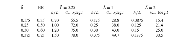


 h=10
 L=40
 L~=1
 x=−127.5mm
 x=42.5mm
 x=357.5mm
 t=0

 L~=0.25,1

 θmax
 (L~,h~)
 MI=1.4
 h~=(L~/π)tanθtr
 θtr≈48∘

 MI=1.4
 x~=−2.5
 t=0.1ms
 t=0.2ms
 t=0.3ms
 L~=0.25, 1, 2

 L~=0.25, 0.5, 0.75, 1
 M=1

 x=0
 P2
 L~=0.25, 1, 2
 P2

 t=1ms
 L~=
 MI

 t=2ms
 L~=
 MI

 MI=1.4
 t=1

 L~
 MI=1.4
 1.8
 L~=0.25
 1
 2
 95%
 ∘
 ×
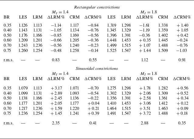
 MI=1.4
 1.8
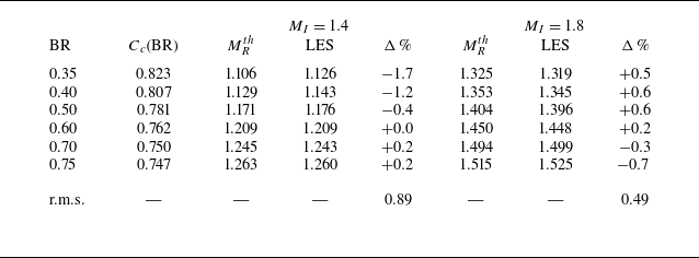
 Cc(BR)

 L~
 MI=1.4
 1.8
 L~=0.25
 1
 2
 95%
 ⋄
 ∗
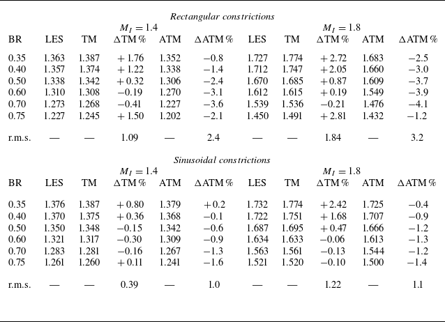
 L~=2
 Cc

 L~=2
 MI=1.4
 BR=0.5
 BR=0.75
 t=0
 2

 L~=2
 MI=1.4
 t=0
 2
 Mavg
 Mmid
 MT∞

 t=1
 Δxmin=250,160,110μm
 BR=0.5
 h=10mm
 L~=1
 L=40mm

 L~=2
 h=5
 h=6
 t=20,50,80,110μ
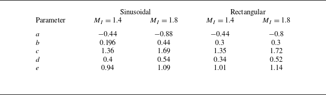

 X(α,t)
 xfb
 xft
 α
 n^=(cosθ,sinθ)
 m^=(−sinθ,cosθ)
 θ
 θghost=2φw−θend
 φw
 φw=0


 Open access

