1 Introduction
Contaminants released from a localised steady source into atmosphere typically advect along the mean wind or streamwise (
 $x$
) direction, and spread in both the vertical (
 $z$
) and transverse (
 $y$
) directions due to turbulent motions. As the plume spreads, the local concentration (typically in parts per million or volume fraction) reduces, and if the contaminant is hazardous then it is desired that the local concentration is within safe limits when it comes in contact with humans, livestock or plants. The magnitude of concentration however changes continuously, and the background turbulent flow imposes a range of time scales on to the scalar field. Likewise, the instantaneous spatial distribution of concentration also has a range of length scales. Thus, at a fixed location, although the concentration might be safe at a particular time instance, it may exceed the safe limit at another time. This manuscript focuses on time scales for concentration and the dependence of concentration (
 $\tilde{C}(t)$
) on different time scales or frequency (
 $f$
) as characterised by the spectrum of concentration,
 $\unicode[STIX]{x1D6F7}_{cc}(f)$
, such that
 $$\begin{eqnarray}\displaystyle \unicode[STIX]{x1D70E}_{c}^{2}=\int _{0}^{\infty }\unicode[STIX]{x1D6F7}_{cc}(f)\,\text{d}f, & & \displaystyle\end{eqnarray}$$
where the instantaneous concentration,
 $\tilde{C}$
is decomposed into mean (
 $C$
) and fluctuating (
 $c$
) components (
 $\tilde{C}=C+c$
), and
 $\unicode[STIX]{x1D70E}_{c}^{2}$
is the concentration variance.
Due to its practical importance, many studies have calculated the concentration spectra (
 $\unicode[STIX]{x1D6F7}_{cc}$
) in both controlled field experiments (Sawford, Frost & Allan Reference Sawford, Frost and Allan1985; Hanna & Insley Reference Hanna and Insley1989) as well as in laboratory conditions (Fackrell & Robins Reference Fackrell and Robins1982a
; Nironi et al.
Reference Nironi, Salizzoni, Marro, Mejean, Grosjean and Soulhac2015; Talluru, Philip & Chauhan Reference Talluru, Philip and Chauhan2018). In all these experiments, a steady source of passive scalar plume is released in a turbulent boundary layer, and concentration is measured at a particular location of interest. Due to obvious limitations of field measurements, recordings are made only at few locations. However, it is of interest to estimate spectra at different locations along or across the plume trajectory. This study outlines a method for such an estimation based on the information of spectrum at one location obtained from a point measurement, and plume characteristics, such as the plume width and the variance distribution.
The spectrum of a passive scalar is of interest for theoretical understanding too (see Corrsin Reference Corrsin1951; Panofsky & Dutton Reference Panofsky and Dutton1984; Sreenivasan Reference Sreenivasan1996; Shraiman & Siggia Reference Shraiman and Siggia2000; Warhaft Reference Warhaft2000, for example), where it is usual to consider the spatial spectrum of concentration,
 $E_{cc}(k)$
(where
 $k$
is the spatial streamwise wavenumber), as opposed to the temporal spectrum
 $\unicode[STIX]{x1D6F7}_{cc}(f)$
defined previously, although the two have similar characteristics (Tennekes & Lumley Reference Tennekes and Lumley1972). It is well known that in the ‘inertial regime’ of turbulence,
 $E_{cc}(k)$
takes the self-similar form,
 $E_{cc}(k)=\unicode[STIX]{x1D6FC}\unicode[STIX]{x1D700}_{c}\unicode[STIX]{x1D700}_{u}^{-1/3}k^{-5/3}$
, where
 $\unicode[STIX]{x1D700}_{c}$
and
 $\unicode[STIX]{x1D700}_{u}$
are respectively the mean concentration and velocity dissipation rates and
 $\unicode[STIX]{x1D6FC}$
is expected to be a universal constant (Corrsin Reference Corrsin1951; Tennekes & Lumley Reference Tennekes and Lumley1972; Sreenivasan Reference Sreenivasan1996). Experiments to validate this form of
 $E_{cc}(k)$
and determine
 $\unicode[STIX]{x1D6FC}$
are typically carried out in isotropic turbulence with a uniform or linearly varying mean scalar field; sometimes the velocity field can have an uniform shear. It is well documented that the approach to a universal form of
 $E_{cc}(k)$
or constant
 $\unicode[STIX]{x1D6FC}$
is Reynolds number dependent with a relatively slower approach in shear flows (Sreenivasan Reference Sreenivasan1996).
In the case of point-source plumes, which is the focus of this study, there are a few models for the concentration spectrum (e.g. Panofsky & Dutton Reference Panofsky and Dutton1984; Hanna Reference Hanna1986; Hanna & Insley Reference Hanna and Insley1989). Through theoretical analysis, Panofsky & Dutton (Reference Panofsky and Dutton1984) have predicted that, over a band of relatively high frequencies (inertial subrange), the fluctuation spectrum should display a
 $f^{-2/3}$
power law when
 $f\unicode[STIX]{x1D6F7}_{cc}$
is plotted against
 $f$
. This result is equivalent to
 $k^{-5/3}$
power law in the narrow inertial subrange of
 $\unicode[STIX]{x1D6F7}_{cc}$
, as discussed earlier. Such a behaviour is universally observed in the spectra of velocity fluctuations in many different turbulent flows at high Reynolds numbers, as reported in numerous studies and textbooks (Tennekes & Lumley Reference Tennekes and Lumley1972; Hinze Reference Hinze1975; Schlichting Reference Schlichting1979; Saddoughi & Veeravalli Reference Saddoughi and Veeravalli1994; Sreenivasan & Antonia Reference Sreenivasan and Antonia1997; Pope Reference Pope2001; Djenidi & Antonia Reference Djenidi and Antonia2012, and references therein). In the case of a narrow meandering plume, the on/off type of signal in concentration due to the passing of puffs of concentration (intermittency) can sometime contribute significantly to the low frequency regime of
 $\unicode[STIX]{x1D6F7}_{cc}$
.
Another prominent model for spectra is the two time scale model due to Hanna (Reference Hanna1986), based on a Markov process, and takes consideration of external intermittency. This is further discussed towards the end of this paper (cf. § 5.2). Importantly, Hanna’s (Reference Hanna1986) model predicts
 $f\unicode[STIX]{x1D6F7}_{cc}\propto f^{-1}$
rather than
 $f\unicode[STIX]{x1D6F7}_{cc}\propto f^{-2/3}$
as suggested by Panofsky & Dutton (Reference Panofsky and Dutton1984). Hanna & Insley (Reference Hanna and Insley1989) have analysed various experimental datasets obtained in the laboratory and atmospheric boundary layers with a view to testing the above models for concentration spectra. They found that the accuracy of Markov spectrum model improves when a second Markov spectrum is combined with the first Markov spectrum using a weighted function based on external intermittency. On the other hand, most of the experimental data agreed very well with the
 $f^{-2/3}$
power law model for the inertial subrange of
 $f\unicode[STIX]{x1D6F7}_{cc}$
. Later studies, such as Fackrell & Robins (Reference Fackrell and Robins1982a
), Mylne, Davidson & Thomson (Reference Mylne, Davidson and Thomson1996) have provided evidence in favour of
 $f^{-2/3}$
power law model. To arrive at this result, Mylne et al. (Reference Mylne, Davidson and Thomson1996) had to perform a de-filtering process of the data obtained using a TIP (total ionisables present) photo-ionisation detector to account for smoothing effects of the instrument due to the finite volume of the ionisation chamber. Importantly, in most studies, such as Fackrell (Reference Fackrell1980), Fackrell & Robins (Reference Fackrell and Robins1982a
), Mylne et al. (Reference Mylne, Davidson and Thomson1996), Nironi et al. (Reference Nironi, Salizzoni, Marro, Mejean, Grosjean and Soulhac2015), the spectrum is presented in wavenumber (
 $k$
) space by invoking Taylor’s ‘frozen-turbulence’ hypothesis to convert frequency
 $f$
to
 $k$
as
 $k=f/U$
, where
 $U$
is the local mean velocity. Hanna (Reference Hanna1986) highlights that, although Taylor’s hypothesis is shown to be valid for velocity spectra, there is no such evidence for concentration spectra. The authors agree with this assessment, and for this reason, the results presented in this paper will be represented in the frequency domain.
As clearly evident, the above models for concentration spectra only describe the behaviour in the inertial subrange. The spectrum model of Hanna (Reference Hanna1986) incorporated the effect of flow turbulence causing meandering of the plume, albeit inadequately. Moreover, the peak in the concentration spectrum for point-source plumes typically appears at lower wavenumbers or frequencies, and is not captured by inertial regime models. In addition to this, the point-source plume is highly inhomogeneous, and the energetic lower frequency contributions of the spectrum are challenging to capture. The present study is further complicated by the fact that the plumes are released in a turbulent boundary layer (TBL), which is neither isotropic nor does it have uniform shear. Physically, the passive scalar is dictated by the background velocity field, as suggested by the phenomenological meandering plume model of Gifford (Reference Gifford1959) and more recent updates (e.g. Weil Reference Weil and Fernando2012; Talluru et al.
Reference Talluru, Philip and Chauhan2018). However, it should be noted that, as the passive concentration is dispersed by the velocity field,
 $\unicode[STIX]{x1D6F7}_{cc}$
depends not only on the various characteristics of the background velocity field, but also on the source geometry, source height and the downstream location. In this study, we primarily investigated the effect of source height and source distance on concentration spectra. For this, we have performed a range of experiments to measure instantaneous concentration in the vertical and transverse directions across the plume, when the plume is released at different heights in the TBL as well as at various upstream locations. Our measurements reveal that the concentration spectrum exhibits a self-similar behaviour. The observed self-similarity implies that it is possible to measure the spectrum at one position in the plume and estimate the spectrum at any other position, given some averaged quantities; this is of much interest in practical applications. To our knowledge, this is the first time such detailed experiments have been performed and data have been used to test self-similarity of concentration spectra.
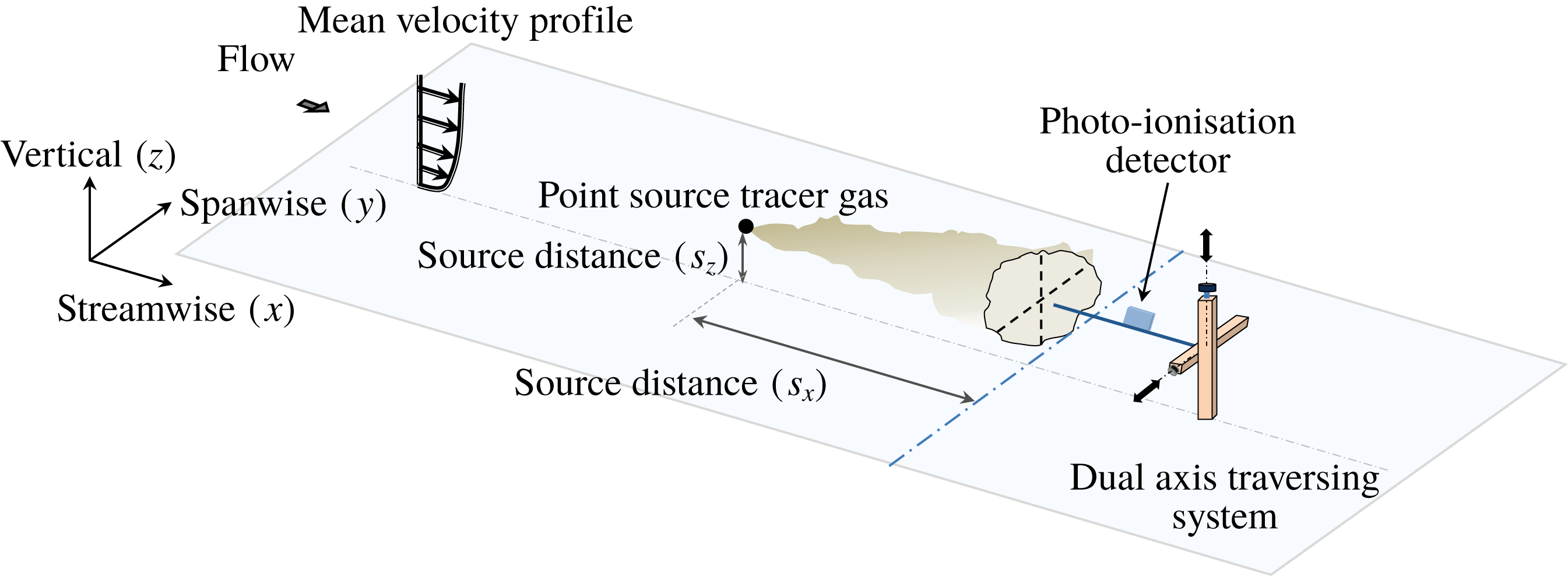
Schematic of experimental set-up used for measuring concentration fluctuations in the transverse (
 $y$
) and vertical (
 $z$
) directions.

2 Experimental details
Experiments are carried out in the Boundary Layer Wind Tunnel (BLWT) at the University of Sydney, where the turbulent boundary layer (TBL) develops over a smooth surface at a free-stream velocity of
 $10~\text{m}~\text{s}^{-1}$
. Details of the facility are available in Talluru et al. (Reference Talluru, Hernandez-Silva, Philip and Chauhan2017a
). The resultant boundary layer thickness
 $\unicode[STIX]{x1D6FF}=0.31~\text{m}$
and friction velocity,
 $U_{\unicode[STIX]{x1D70F}}=0.37~\text{m}~\text{s}^{-1}$
are determined by matching the logarithmic mean velocity profile to the constants
 $\unicode[STIX]{x1D705}=0.384$
and
 $A=4.17$
(Chauhan, Nagib & Monkewitz Reference Chauhan, Nagib and Monkewitz2009). This yields a friction Reynolds number,
 $Re_{\unicode[STIX]{x1D70F}}=\unicode[STIX]{x1D6FF}^{+}=\unicode[STIX]{x1D6FF}U_{\unicode[STIX]{x1D70F}}/\unicode[STIX]{x1D708}\approx 7850$
(where
 $\unicode[STIX]{x1D708}$
is the kinematic viscosity). A tracer gas (mixture of 98.5 % nitrogen and 1.5 % iso-butylene) is released through a discharge tube emulating a point source at eight source heights (
 $s_{z}$
) and four source distances (
 $s_{x}$
) as illustrated in figure 1. Most of the results presented in the paper are for
 $s_{x}/\unicode[STIX]{x1D6FF}=1$
, although sometimes we employed data from
 $s_{x}/\unicode[STIX]{x1D6FF}=0.5,2$
and
 $4$
. For each
 $s_{x}/\unicode[STIX]{x1D6FF}$
and
 $s_{z}/\unicode[STIX]{x1D6FF}$
we measure concentration in both the vertical (
 $z$
) and spanwise (
 $y$
) directions.
The tracer gas is released iso-kinetically into the flow by matching the source velocity (
 $U_{s}$
) with the local boundary layer mean velocity at
 $z=s_{z}$
. The diameter of the source (
 $s_{d}$
) is approximately 1.6 mm and the ratio of source size to boundary layer thickness is
 $s_{d}/\unicode[STIX]{x1D6FF}=0.005$
. This clearly indicates that the source can be treated as a point source and the plume as slender. Concentration is measured using a photo-ionisation detector (PID) at multiple locations in
 $y$
and
 $z$
. The sensor size of the PID is 0.76 mm, which is shown to be smaller than
 $10\unicode[STIX]{x1D702}_{c}$
(Kolmogorov microscale of concentration) and hence, has minimal effect on the spectra. Full details of the sensor and its calibration can be found in Talluru et al. (Reference Talluru, Hernandez-Silva, Philip and Chauhan2017a
), Talluru, Hernandez-Silva & Chauhan (Reference Talluru, Hernandez-Silva and Chauhan2019). The frequency response of the PID sensor is experimentally estimated to be approximately 400 Hz (see Talluru et al.
Reference Talluru, Hernandez-Silva, Philip and Chauhan2017b
, for details). At each measurement point, samples are collected for a duration of 300 seconds at a sampling rate of 4096 Hz. Throughout this paper, flow variables with capitalised letters (e.g.
 $C$
) denote time-averaged quantities, whereas lower case letters (e.g.
 $c$
) indicate fluctuating quantities.
A dual-axis traverse is used to acquire concentration measurements in the spanwise (
 $y$
) and vertical (
 $z$
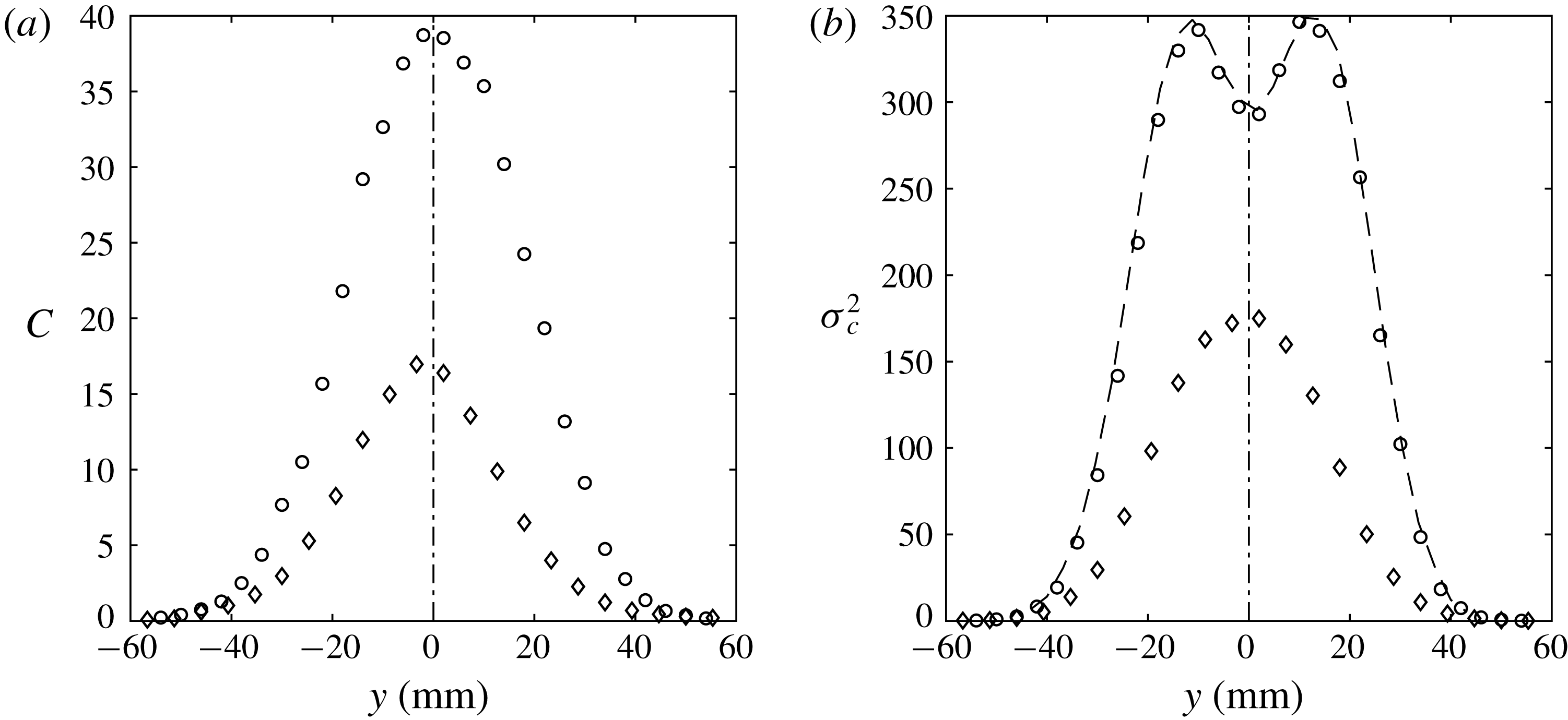
) directions across the plume. The traverse is driven by two stepper motors, each fitted with an optical encoder of one-micron resolution. In our initial experiments, we investigated the symmetry in the mean and variance profiles of concentration in the transverse direction at
 $s_{x}/\unicode[STIX]{x1D6FF}=1$
. The results of mean concentration (
 $C$
) and variance (
 $\unicode[STIX]{x1D70E}_{c}^{2}$
) for a ground level and an elevated source plume are shown in figure 2(a,b), respectively. These clearly suggest that there is the expected symmetry along
 $y$
-direction in the plume. Hence, measurements are only conducted on one side of the plume in the transverse direction.
Profiles of (a) mean and (b) variance of concentration across the entire plume in the transverse (
 $y$
) direction for a ground level (
 $s_{z}/\unicode[STIX]{x1D6FF}=0.004=32/\unicode[STIX]{x1D6FF}^{+}$
; ○) and an elevated source (
 $s_{z}/\unicode[STIX]{x1D6FF}=0.25$
; ♢) plume. The vertical dot-dashed lines indicate the plume centreline. Note that
 $\unicode[STIX]{x1D6FF}^{+}=\unicode[STIX]{x1D6FF}U_{\unicode[STIX]{x1D70F}}/\unicode[STIX]{x1D708}=7850$
. The black dashed line in (b) is generated using (4.4) (of Sawford & Sullivan Reference Sawford and Sullivan1995) with
 $\unicode[STIX]{x1D6FC}=1.3$
and
 $\unicode[STIX]{x1D6FD}=0.78$
.

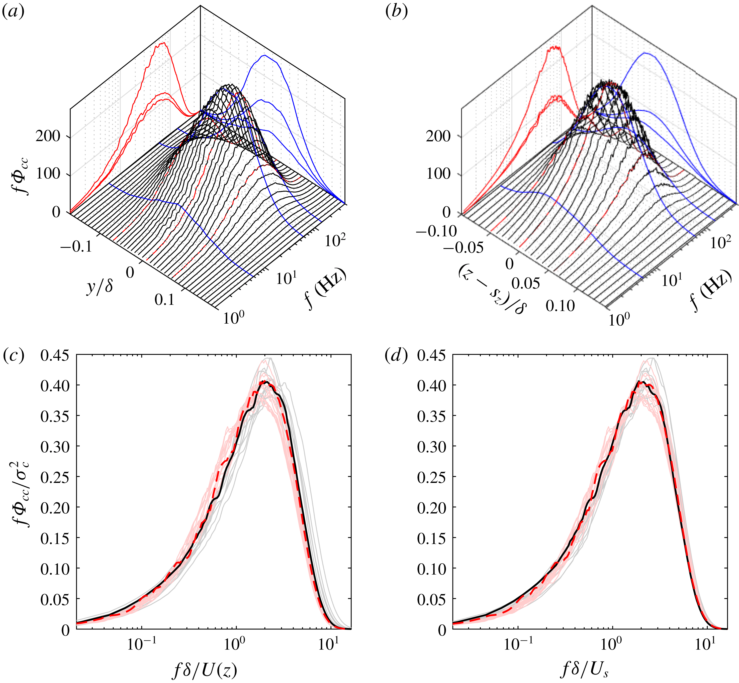
Pre-multiplied spectra of concentration across the plume released at
 $s_{z}/\unicode[STIX]{x1D6FF}=0.1$
as a function of frequency and (a) spanwise coordinate
 $y$
; (b) wall-normal coordinate
 $z$
. Blue curves represent the spectra at three (arbitrary) frequencies; 6, 60 and 150 Hz. Red curves show the spectra on the centreline of plume and the two
 $z$
-locations, where
 $\unicode[STIX]{x1D70E}_{c}^{2}$
is equal to half of the centreline value,
 $\unicode[STIX]{x1D70E}_{c,ref}^{2}$
. (c) Pre-multiplied spectra at different
 $y$
-locations (light-red lines) and
 $z$
-locations (grey lines) of the plume. Dashed-red and solid-black lines are the measurements at the plume centreline obtained in the spanwise and wall-normal profiles. Frequency is normalised using boundary layer thickness (
 $\unicode[STIX]{x1D6FF}$
) and local mean velocity (
 $U$
). (d) Same as (c) with source velocity (
 $U_{s}$
) used to normalise frequency.

3 Self-similarity of concentration spectra
Figure 3(a,b) shows a three-dimensional overview of pre-multiplied spectra,
 $f\unicode[STIX]{x1D6F7}_{cc}$
, along
 $y$
- and
 $z$
-directions, respectively, for a plume released at
 $s_{z}/\unicode[STIX]{x1D6FF}=0.1$
. Axes for spectra and frequency are intentionally kept dimensional as their appropriate non-dimensionalisation is discussed in the following. First, consider the distribution of
 $f\unicode[STIX]{x1D6F7}_{cc}$
at three different
 $y$
-locations in figure 3(a), i.e. the plume centreline and the two other spanwise locations where
 $\unicode[STIX]{x1D70E}_{c}^{2}$
is half the plume centreline value. These distributions are shown as red lines on the side vertical plane of figure 3(a). From this representation, it is seen that
 $f\unicode[STIX]{x1D6F7}_{cc}$
at these three locations have similar shapes, however, with different areas under the individual curves. Note that area under these curves is equal to the corresponding variance
 $\unicode[STIX]{x1D70E}_{c}^{2}$
, as mentioned earlier in § 1; and for this reason, two of the three curves are identical since they have the similar magnitude of
 $\unicode[STIX]{x1D70E}_{c}^{2}$
. A similar behaviour is noticed for concentration spectra from measurements along the
 $z$
-direction of the plume in figure 3(b).
3.1 Velocity and length scales for self-similarity
Self-similarity of spectra requires suitable normalisation of
 $f\unicode[STIX]{x1D6F7}_{cc}$
and
 $f$
such that black lines in figure 3(a,b) collapse to agree well with a representative spectrum. Extensive examination of data in our experimental campaign has consistently indicated that the shape of
 $f\unicode[STIX]{x1D6F7}_{cc}$
at various locations is similar and only differs by the area under the curves, i.e.
 $\unicode[STIX]{x1D70E}_{c}^{2}$
. Hence,
 $f\unicode[STIX]{x1D6F7}_{cc}$
for each spectrum is non-dimensionalised by the corresponding
 $\unicode[STIX]{x1D70E}_{c}^{2}$
in figure 3(c,d) so that the area under each curve equals one. Normalisation of frequency requires a time scale and for single-point Eulerian measurements, a time scale is typically constructed using a velocity scale (
 ${\mathcal{U}}$
) and length scale (
 ${\mathcal{L}}$
) such that
 ${\mathcal{L}}/{\mathcal{U}}$
has dimensions of seconds. For a plume in a turbulent boundary layer, two relevant velocity scales are the local velocity
 $U$
(where the concentration is measured) and the source velocity
 $U_{s}:=U(z=s_{z})$
. Note that the scaling of frequency with local mean velocity (
 $U$
) has been done in previous studies such as Fackrell & Robins (Reference Fackrell and Robins1982a
), Nironi et al. (Reference Nironi, Salizzoni, Marro, Mejean, Grosjean and Soulhac2015). Since
 $U$
is a function of
 $z$
, the scaling of frequency with
 $U$
inherently has a dependence on
 $z$
. Such a scaling has resulted in good collapse of velocity spectra in a turbulent boundary layer (see Baidya et al.
Reference Baidya, Philip, Hutchins, Monty and Marusic2017, for example). Here,
 $U$
is being tested as a velocity scale to see if it leads to a collapse of concentration spectra.
Figure 3(c,d) shows the normalised distributions using
 $f\unicode[STIX]{x1D6FF}/U$
and
 $f\unicode[STIX]{x1D6FF}/U_{s}$
, respectively. Light-grey and light-red lines indicate the spectra from figure 3(a,b) in normalised form at different
 $y$
and
 $z$
locations. It is evident that they have very similar shapes to that of spectra at the plume centreline (shown by solid-black and dashed-red lines) providing experimental evidence for the self-similar behaviour of concentration spectra. Although the normalised spectrum at the plume centreline is chosen as reference for comparison, it can be justifiably replaced by a concentration spectrum at any other location in the plume. Notice that both
 $U$
and
 $U_{s}$
are reasonably good candidates; however,
 $U_{s}$
results in marginally better overall collapse. It may be argued that other choices of velocity scale, such as
 $U_{\infty }$
and
 $U_{\unicode[STIX]{x1D70F}}$
, will also lead to collapse of spectra since the three velocity scales (
 $U_{s}$
,
 $U_{\infty }$
and
 $U_{\unicode[STIX]{x1D70F}}$
) are all constant for a given flow configuration and source height. Previous estimates of convection velocities of coherent structures in a turbulent boundary layer have shown that instantaneous motions are convected at a velocity that is of the order of the local mean velocity (e.g. del Álamo & Jiménez Reference del Álamo and Jiménez2009). Since the instantaneous transport of the scalar is due to local turbulence, the convection velocity of the scalar will be similar to that of the turbulent motions, i.e. the mean velocity, as opposed to
 $U_{\unicode[STIX]{x1D70F}}$
or
 $U_{\infty }$
. Furthermore,
 $U_{s}$
is a preferred choice as it is convenient to measure it in practical situations, for instance, based on the emission rate of smoke from a tall stack. On the other hand, it is much more difficult to measure
 $U_{\infty }$
(which might not even exist in an atmospheric flow) and
 $U_{\unicode[STIX]{x1D70F}}$
(or the ‘roughness length’) in the atmospheric boundary layer.
At this point, it is important to discuss the relevance of
 $U_{s}$
as an appropriate velocity scale for scaling concentration spectra. In the present study, the measurements are limited to
 $s_{x}/\unicode[STIX]{x1D6FF}\leqslant 4$
and the maximum plume width in this region is found to be less than 10 % of the boundary layer thickness. This implies that the investigation here is limited to narrow plumes, and so, it is expected that the growth of the plume is dictated by the source conditions, namely the mean velocity and the turbulence intensity at the source location (Fackrell & Robins Reference Fackrell and Robins1982b
; Nironi et al.
Reference Nironi, Salizzoni, Marro, Mejean, Grosjean and Soulhac2015). This is the reason why we observe a good collapse when
 $U_{s}$
is used as a velocity scale. However, in the far-field region, where the plume is thoroughly mixed across the entire boundary layer, it is possible that plume development is governed by a wide range of velocity scales present in the flow. The lack of such data in the literature to test self-similarity of concentration spectra in the far-field region provides scope for future study.
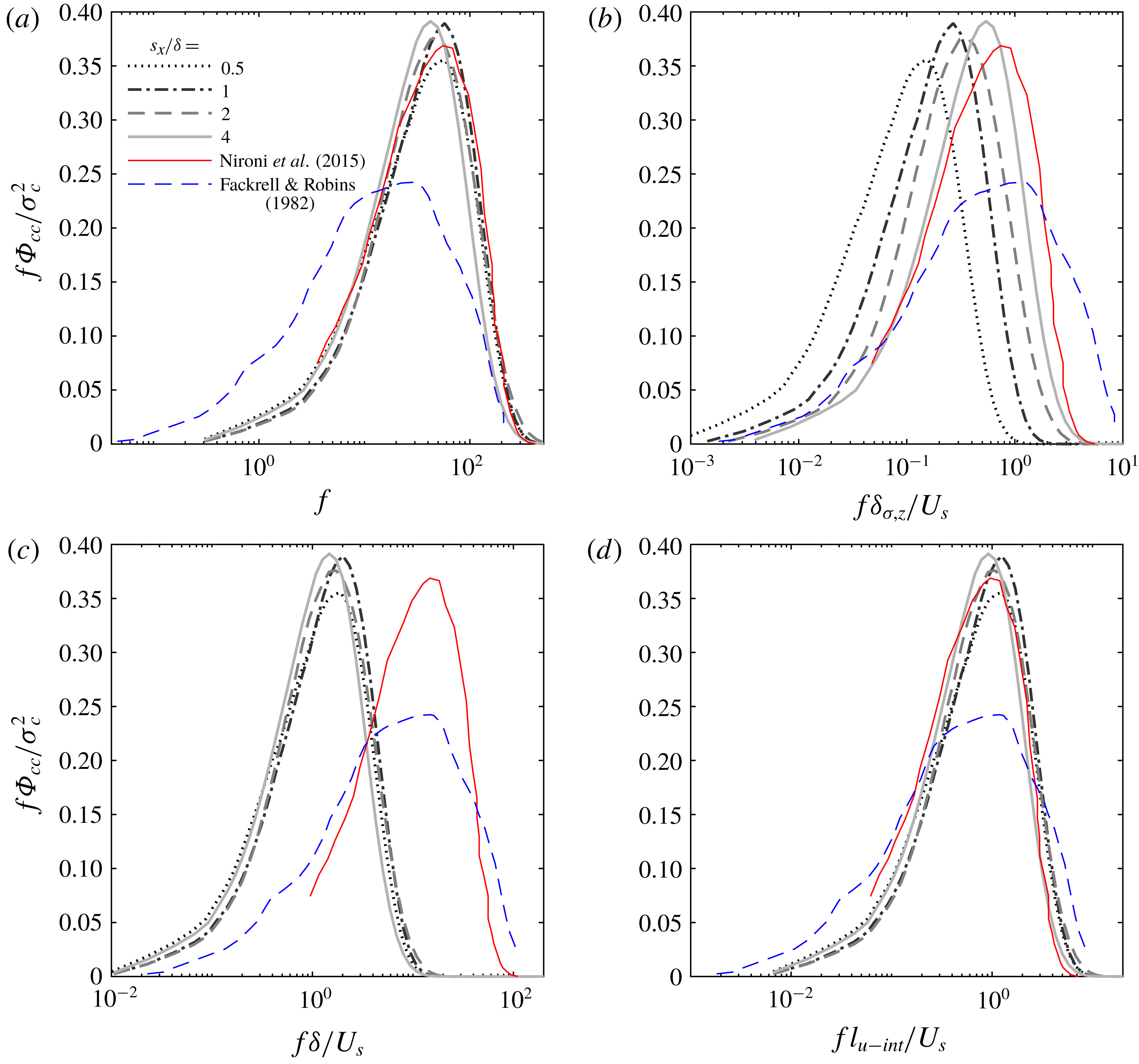
Comparison of normalised spectra of concentration at the plume centreline using (a) dimensional frequency; three different length scales – (b) half-plume width
 $\unicode[STIX]{x1D6FF}_{\unicode[STIX]{x1D70E},z}$
; (c) boundary layer thickness
 $\unicode[STIX]{x1D6FF}$
and (d) integral length scale
 $l_{u-int}$
and source velocity
 $U_{s}$
as velocity scale for four source distances,
 $s_{x}/\unicode[STIX]{x1D6FF}=0.5$
, 1, 2 and 4, and at a fixed height,
 $s_{z}/\unicode[STIX]{x1D6FF}=0.1$
. Note that the data of Fackrell & Robins (Reference Fackrell and Robins1982a
) and Nironi et al. (Reference Nironi, Salizzoni, Marro, Mejean, Grosjean and Soulhac2015) used here are digitally extracted from the respective papers.

The choice of
 ${\mathcal{L}}=\unicode[STIX]{x1D6FF}$
in figure 3(c,d) also requires further discussion on the appropriate length scale to be employed in scaling frequency. Three different length scales are investigated in figure 4 for the plume released at
 $s_{z}/\unicode[STIX]{x1D6FF}=0.1$
and four different streamwise locations (
 $s_{x}/\unicode[STIX]{x1D6FF}$
). Here we also include data from Fackrell & Robins (Reference Fackrell and Robins1982a
) and Nironi et al. (Reference Nironi, Salizzoni, Marro, Mejean, Grosjean and Soulhac2015), where a localised passive scalar plume was released in turbulent boundary layers over rough surfaces. We note that data from Fackrell & Robins (Reference Fackrell and Robins1982a
) show a lower amplitude compared to other data, which is likely due to the limitations of the sensor employed in the 1980s.
Figure 4(a) shows the abscissa in dimensional frequency in Hz, whereas we test three different length scales in figure 4(b,c,d), respectively, the plume (variance) thickness in the vertical direction
 $\unicode[STIX]{x1D6FF}_{\unicode[STIX]{x1D70E},z}$
(where variance reduces to half its maximum value), the boundary layer thickness
 $\unicode[STIX]{x1D6FF}$
and the velocity integral length scale
 $l_{u-int}:=\int R_{uu}(x)\,\text{d}x$
(where,
 $R_{uu}$
is the normalised autocorrelation function of the streamwise velocity). Here,
 $l_{u-int}$
is calculated by integrating the autocorrelation function
 $R_{uu}(x)$
in the interval
 $0\leqslant x/\unicode[STIX]{x1D6FF}\leqslant 20$
following the approach of Talluru et al. (Reference Talluru, Philip and Chauhan2018). Note that here we are testing variance half-width, rather than the plume width based on mean concentration (traditionally used in the atmospheric science community) as a length scale, because the focus of this study is the scaling of concentration spectra, which is directly linked to the variance (cf. (1.1)). It is clear from figure 4(b) that
 $\unicode[STIX]{x1D6FF}_{\unicode[STIX]{x1D70E},z}$
is not an appropriate length scale; in fact, none of the ‘plume’ length scales (which were sometimes used in the past, e.g. Hanna & Insley Reference Hanna and Insley1989) are suitable for the scaling purposes. This is perhaps not surprising, since it known that passive plume length scales are dictated by the background velocity field length scales (e.g. Gifford Reference Gifford1959; Talluru et al.
Reference Talluru, Philip and Chauhan2018). For our data figure 4(a,c,d) shows good collapse. This is because, for the present study,
 $\unicode[STIX]{x1D6FF}$
is a constant, and it is known that
 $l_{u-int}$
is proportional to
 $\unicode[STIX]{x1D6FF}$
in the outer part of a TBL (e.g. Hutchins & Marusic Reference Hutchins and Marusic2007). Inclusion of other data from rough-wall TBL, however, shows that
 $l_{u-int}$
is a more appropriate length scale (cf., figure 4
d). In rough-wall flows the roughness can introduce its own length scales that need not be proportional to
 $\unicode[STIX]{x1D6FF}$
. In fact, as a practical advantage for
 $l_{u-int}$
, in atmospheric flows it is more convenient to measure
 $l_{u-int}$
because it depends on the local flow conditions, and can be measured with relative ease compared to
 $\unicode[STIX]{x1D6FF}$
that requires the knowledge of the entire BL. In the rest of the paper, however, we continue to use
 $\unicode[STIX]{x1D6FF}$
because of its constancy, and because both
 $\unicode[STIX]{x1D6FF}$
and
 $l_{u-int}$
show almost identical results.
3.2 Self-similarity of spectra across the plume cross-section (
 $y$
-
$z$
plane) at a particular frequency


In the previous section § 3.1, we discussed the ‘usual kind of self-similarity’ of spectra that is studied in most plume investigations. There, the typical aim is to scale the spectral amplitude and frequency appropriately so as to collapse all the available spectra data onto to a ‘universal’ curve, which can then be employed for prediction if we know the scaling variables (such as
 $\unicode[STIX]{x1D70E}_{cc}$
for amplitude, and
 $\unicode[STIX]{x1D6FF}$
or
 $l_{u-int}$
and
 $U_{s}$
for frequency). In this section, we discuss self-similarity of a slightly different kind, one that we realised almost serendipitously from the three-dimensional figure 3(a,b). We refer back to the blue lines on the rear panels in figure 3(a,b), which are distributions of
 $\unicode[STIX]{x1D6F7}_{cc}$
as a function of
 $y$
or
 $z$
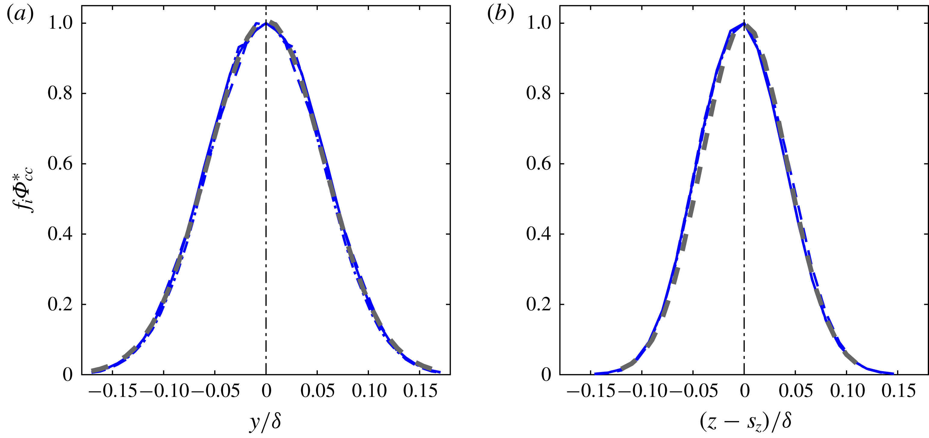
at three arbitrary frequencies: 6, 60 and 150 Hz. These curves are replotted in figure 5(a,b) after normalising by the respective maxima, i.e.
 $f_{i}\unicode[STIX]{x1D6F7}_{cc}^{\ast }=f_{i}\unicode[STIX]{x1D6F7}_{cc}/\text{max}(f_{i}\unicode[STIX]{x1D6F7}_{cc}),i=6$
, 60 and 150 Hz. It is clearly evident that
 $f_{i}\unicode[STIX]{x1D6F7}_{cc}^{\ast }(x,y,z)$
collapses on to a single curve and has a Gaussian behaviour. The (grey) dashed lines are Gaussian curves plotted in figures 5(a,b), and they are indistinguishable from the data.
(a,b) Blue curves shown in figure 3(a,b) are replotted here after normalising by the maxima (
 $f_{i}\unicode[STIX]{x1D6F7}_{cc}^{\ast }$
,
 $i=6$
, 60 and 150 Hz). Grey dashed lines are the Gaussian curves and the vertical dot-dashed lines represent the plume centreline.

The above similarity is equally valid at all frequencies such that both
 $f\unicode[STIX]{x1D6F7}_{cc}(x,y,z)$
and
 $\unicode[STIX]{x1D70E}_{c}^{2}(x,y,z)$
follow the same spatial distribution. For a fixed
 $x$
and
 $z$
, the similarity model can be written as,
 $$\begin{eqnarray}\displaystyle {\displaystyle \frac{f\unicode[STIX]{x1D6F7}_{cc}(f,y)}{\unicode[STIX]{x1D70E}_{c}^{2}(y)}}=g(f)\quad \Rightarrow \quad {\displaystyle \frac{f\unicode[STIX]{x1D6F7}_{cc}(f,y_{1})}{\unicode[STIX]{x1D70E}_{c}^{2}(y_{1})}}={\displaystyle \frac{f\unicode[STIX]{x1D6F7}_{cc}(f,y_{2})}{\unicode[STIX]{x1D70E}_{c}^{2}(y_{2})}}, & & \displaystyle\end{eqnarray}$$
to within experimental uncertainty, where,
 $g(f)$
is some arbitrary function of frequency only (or a reference spectrum from figure 3
d),
 $y_{1}$
and
 $y_{2}$
are two arbitrary spanwise locations and a similar expression holds in the
 $z$
-direction. Importantly, this shows that at each frequency, the concentration energy (
 $\unicode[STIX]{x1D6F7}_{cc}$
) is distributed across the
 $y$
and
 $z$
-directions and is proportional to
 $\unicode[STIX]{x1D70E}_{c}^{2}$
at that location. This is a strong indication that the meandering nature of the plume, which is the reason for the variance distribution to be Gaussian (Gifford Reference Gifford1959), is also likely to be responsible for imposing a uniform bandwidth of frequencies in concentration spectra at all locations across the plume. Thus, it is important to note here that the observed self-similar behaviour of concentration spectra is applicable only for a narrow meandering passive plume. Further, it should be noted that the measurements acquired in this study are for
 $0.5\unicode[STIX]{x1D6FF}\leqslant s_{x}\leqslant 4\unicode[STIX]{x1D6FF}$
, where
 $s_{x}$
is the distance between the point source and the measurements. It is known that a Gaussian shape for the concentration variance is not valid close to the plume source, particularly for
 $s_{x}<0.5\unicode[STIX]{x1D6FF}$
(Sawford & Sullivan Reference Sawford and Sullivan1995), and as such, the model presented here should be deemed not applicable in this region.
A detailed mechanism for the instantaneous meandering and resulting self-similarity is still not completely understood; however, the experimental observations strongly support the meandering nature of the plume. Although the results presented in this study are for slender plumes (i.e. the plume size is nominally less than 10 % of boundary layer thickness), we believe that the analysis is equally valid when the source size is varied as long as it generates a narrow meandering plume. From previous studies (Fackrell & Robins Reference Fackrell and Robins1982a ; Nironi et al. Reference Nironi, Salizzoni, Marro, Mejean, Grosjean and Soulhac2015), it is well known that meandering is caused when the source size is typically smaller than the integral length scale of the background turbulence. And in all such cases, the self-similar behaviour of concentration spectra can be expected.
4 A predictive model
The results in § 3.2 suggest that the spectrum of
 $c$
at a given (
 $x,y,z$
) location can be expressed as a weighted spectrum at the plume centreline with
 $\unicode[STIX]{x1D70E}_{c}^{2}(x,y,z)/\unicode[STIX]{x1D70E}_{c,ref}^{2}$
as the multiplier (consistent with (3.1)):
 $$\begin{eqnarray}\displaystyle & \displaystyle f\unicode[STIX]{x1D6F7}_{cc}(f,y)=\frac{\unicode[STIX]{x1D70E}_{c}^{2}(y)}{\unicode[STIX]{x1D70E}_{c,ref}^{2}}~f\unicode[STIX]{x1D6F7}_{cc}(f,y=0); & \displaystyle\end{eqnarray}$$
 $$\begin{eqnarray}\displaystyle & \displaystyle f\unicode[STIX]{x1D6F7}_{cc}(f,z)=\frac{\unicode[STIX]{x1D70E}_{c}^{2}(z)}{\unicode[STIX]{x1D70E}_{c,ref}^{2}}~f\unicode[STIX]{x1D6F7}_{cc}(f,z=s_{z}), & \displaystyle\end{eqnarray}$$
where,
 $\unicode[STIX]{x1D70E}_{c,ref}^{2}:=\unicode[STIX]{x1D70E}_{c}^{2}(y=0,z=s_{z})$
. Note that the reference location as the plume centreline is simply chosen for convenience, and is not a restriction. Equations (4.1) and (4.2) imply that, to find the spectrum at a location of interest, one requires, (i)
 $\unicode[STIX]{x1D70E}_{c}^{2}$
at that location, and (ii) the spectrum at any other location within the plume, which we take for convenience as the plume centreline. From a practical point of view, there are many models that can predict
 $\unicode[STIX]{x1D70E}_{c}^{2}$
variations that are derived from the meandering plume model (Gifford Reference Gifford1959) (see also Weil Reference Weil and Fernando2012), whereas the spectrum at one position is needed from measurements. More recently, high-order closure models (Yee, Wang & Lien Reference Yee, Wang and Lien2009) and PDF (probability density function) micro-mixing models (e.g. Cassiani, Franzese & Giostra Reference Cassiani, Franzese and Giostra2005; Marro et al.
Reference Marro, Salizzoni, Soulhac and Cassiani2018) have led to better predictions of concentration variance profiles in comparison to the meandering plume model of Gifford (Reference Gifford1959). It is important to note that the predictive model (4.2) is independent of any scaling length or velocity scale, as discussed in § 3.1. In this sense, it is not a conventional predictive model, and although the present model is less restrictive, it only requires measurement at any one location within the plume.
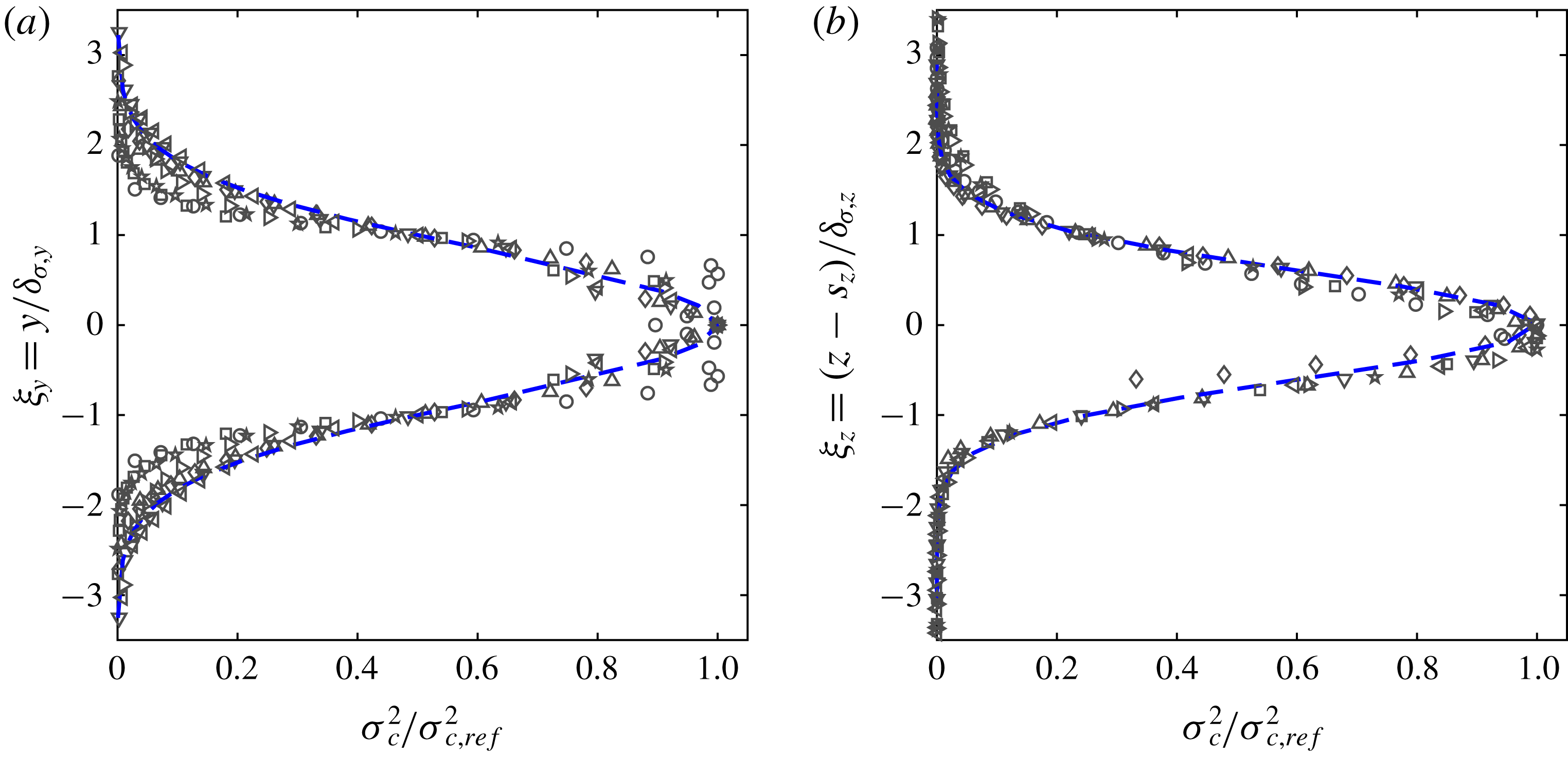
Profiles of normalised variance of concentration as a function of (a)
 $\unicode[STIX]{x1D709}_{y}=y/\unicode[STIX]{x1D6FF}_{\unicode[STIX]{x1D70E},y}$
, and (b)
 $\unicode[STIX]{x1D709}_{z}=(z-s_{z})/\unicode[STIX]{x1D6FF}_{\unicode[STIX]{x1D70E},z}$
. Symbols represent different source heights
 $s_{z}/\unicode[STIX]{x1D6FF}$
: ○ – 32/
 $\unicode[STIX]{x1D6FF}^{+}$
; ♢ – 350
 $/\unicode[STIX]{x1D6FF}^{+}$
; ▵ – 0.1; ▿ – 0.25; ◃ – 0.33; ▹ – 0.5; ▫ – 0.67;
 $\star$
–
 $\unicode[STIX]{x1D6FF}_{99}/\unicode[STIX]{x1D6FF}$
. Dashed-blue lines in (a,b) are the Gaussian profiles given by (4.3).

4.1 Model parameters
Figure 6(a,b) plots the normalised concentration variance as a function of
 $\unicode[STIX]{x1D709}_{y}=y/\unicode[STIX]{x1D6FF}_{\unicode[STIX]{x1D70E},y}$
and
 $\unicode[STIX]{x1D709}_{z}=(z-s_{z})/\unicode[STIX]{x1D6FF}_{\unicode[STIX]{x1D70E},z}$
, respectively for the plume released at different heights. A representative Gaussian profile, in accordance with the meandering plume model (e.g. Gifford Reference Gifford1959; Weil Reference Weil and Fernando2012), for the normalised variance profiles is also plotted in figure 6 and is written as:
 $$\begin{eqnarray}\displaystyle \frac{\unicode[STIX]{x1D70E}_{c}^{2}(y)}{\unicode[STIX]{x1D70E}_{c,ref}^{2}}=\exp \left\{-\text{ln(2)}\left(\frac{y}{\unicode[STIX]{x1D6FF}_{\unicode[STIX]{x1D70E},y}}\right)^{2}\right\};\quad \frac{\unicode[STIX]{x1D70E}_{c}^{2}(z)}{\unicode[STIX]{x1D70E}_{c,ref}^{2}}=\exp \left\{-\text{ln(2)}\left(\frac{z-s_{z}}{\unicode[STIX]{x1D6FF}_{\unicode[STIX]{x1D70E},z}}\right)^{2}\right\}. & & \displaystyle\end{eqnarray}$$
Here, ln(2) is the logarithm of 2. It is used in the above form of Gaussian equation so that
 $\unicode[STIX]{x1D6FF}_{\unicode[STIX]{x1D70E},y}$
or
 $\unicode[STIX]{x1D6FF}_{\unicode[STIX]{x1D70E},z}$
represents the half-plume width in the concentration variance (i.e. at
 $y=\unicode[STIX]{x1D6FF}_{c,y},\unicode[STIX]{x1D70E}_{c}^{2}(y)=(1/2)\unicode[STIX]{x1D70E}_{c,ref}^{2}$
, and similarly in the
 $z$
-direction). Such a representation was previously used by Fackrell & Robins (Reference Fackrell and Robins1982a
). Although the data in figure 6 are in good agreement with (4.3), some differences are observed in
 $\unicode[STIX]{x1D70E}_{c}^{2}(y)$
for a ground level source (shown by ○ symbols in the figures). The distinct behaviour of
 $\unicode[STIX]{x1D70E}_{c}^{2}(y)$
is more clearly seen in figure 2(b) due to less clutter, where two peaks (one on either side of the plume centreline) are observed in the variance profile. Hence, a simple Gaussian model is not adequate to describe such a behaviour. This will be further discussed in a later section. For all other sources, (4.3) is a good fit to the empirical data. Note that (4.2) essentially requires a single parameter, that is, the plume half-width. The variation of plume half-widths
 $\unicode[STIX]{x1D6FF}_{\unicode[STIX]{x1D70E},y}$
and
 $\unicode[STIX]{x1D6FF}_{\unicode[STIX]{x1D70E},z}$
are plotted as a function of source height
 $s_{z}$
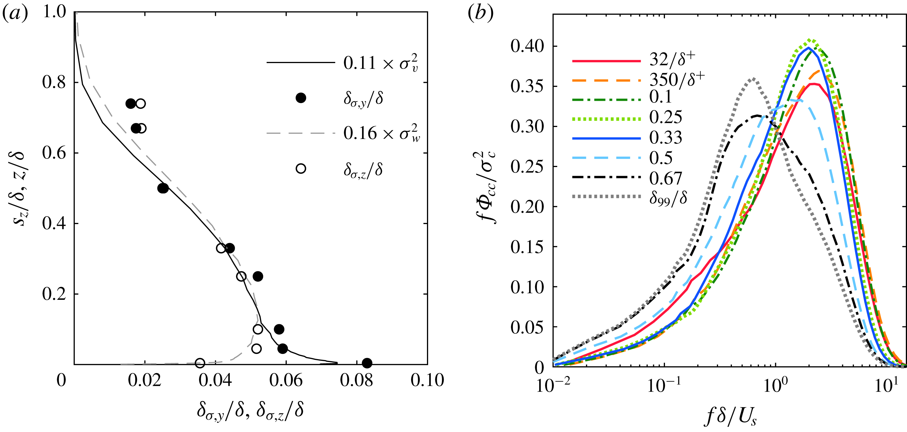
in figure 7(a) as filled and open symbols, respectively. Indeed,
 $\unicode[STIX]{x1D6FF}_{\unicode[STIX]{x1D70E},z}$
depends on
 $s_{x}$
and it is different from the half-plume width based on the mean concentration (
 $\unicode[STIX]{x1D6FF}_{C}$
). Typically the mean concentration profile is relatively easier to predict/calculate with confidence. If one adopts a standardised distribution (probability density functions) for concentration fluctuations (such as gamma functions (Nironi et al.
Reference Nironi, Salizzoni, Marro, Mejean, Grosjean and Soulhac2015)), as typically done in practical applications, one can then easily translate the variance to mean and vice versa and thus work with either of
 $\unicode[STIX]{x1D6FF}_{C}$
or
 $\unicode[STIX]{x1D6FF}_{\unicode[STIX]{x1D70E}}$
. However, the aim of estimating
 $\unicode[STIX]{x1D6FF}_{C}$
or
 $\unicode[STIX]{x1D6FF}_{\unicode[STIX]{x1D70E}}$
as a function of source distance,
 $s_{x}/\unicode[STIX]{x1D6FF}$
is beyond the scope of this study.
As a side point, we compare the plume half-widths with profiles of spanwise and wall-normal velocity variance (
 $\unicode[STIX]{x1D70E}_{v}^{2}$
and
 $\unicode[STIX]{x1D70E}_{w}^{2}$
) measured in our previous study (Talluru et al.
Reference Talluru, Philip and Chauhan2018) in figure 7. Note that the velocity variances are scaled by an arbitrary factor. We find that there is a good agreement between plume half-widths and scaled variance profiles in the respective directions. This result suggests that the plume spread is governed by local turbulence levels at the source height, and thus for practical applications, it might be possible to estimate the plume half-width using turbulence intensities of the background flow which are relatively easier to measure than concentration profiles. The relationship between (Lagrangian) turbulence intensities and the plume width in the respective directions has been previously derived using analytical arguments (Taylor Reference Taylor1922); however, it has not been extensively tested against experimental data. In this regards, the current study provides clear support to the theoretical understanding via the data of plume half-widths in the transverse and vertical directions at eight source locations in a high Reynolds number turbulent boundary layer in figure 6(a). Furthermore,
 $\unicode[STIX]{x1D6FF}_{\unicode[STIX]{x1D70E},y}$
is greater than
 $\unicode[STIX]{x1D6FF}_{\unicode[STIX]{x1D70E},z}$
for
 $s_{z}/\unicode[STIX]{x1D6FF}\leqslant 0.33$
, beyond which the values are quite similar, a behaviour similar to the relative magnitude of
 $\unicode[STIX]{x1D70E}_{v}^{2}$
and
 $\unicode[STIX]{x1D70E}_{w}^{2}$
near the wall, where
 $\unicode[STIX]{x1D70E}_{v}^{2}$
is relatively large compared to
 $\unicode[STIX]{x1D70E}_{w}^{2}$
(e.g. see Talluru et al.
Reference Talluru, Baidya, Hutchins and Marusic2014; Baidya et al.
Reference Baidya, Philip, Hutchins, Monty and Marusic2017, for most recent high-resolution measurements of transverse and lateral velocity fluctuations in a high Reynolds number turbulent boundary layer). A similar reasoning explains the transverse plume width being approximately 25 % larger than the vertical plume width in a uniformly sheared flow (Vanderwel & Tavoularis Reference Vanderwel and Tavoularis2014). The results presented in figure 7(a) clearly support the common modelling practice of using local turbulence at the source height to model plume dispersion in the cross-wind and vertical directions.
The two inputs for the spectrum model. (a) Half-plume widths (
 $\unicode[STIX]{x1D6FF}_{\unicode[STIX]{x1D70E},y}/\unicode[STIX]{x1D6FF}$
,
 $\unicode[STIX]{x1D6FF}_{\unicode[STIX]{x1D70E},z}/\unicode[STIX]{x1D6FF}$
); (b) normalised pre-multiplied spectra of concentration fluctuations at the reference location for all source heights. Solid black and dashed grey lines in (a) represent the variance profiles of spanwise velocity,
 $\unicode[STIX]{x1D70E}_{v}^{2}$
and wall-normal velocity
 $\unicode[STIX]{x1D70E}_{w}^{2}$
, respectively.

The second input to the model is the concentration spectrum measured at a reference location, which is the plume centreline in this study. Normalised spectra at the reference location for eight source heights is shown in figure 7(b). It is found that non-dimensional spectra are similar to each other for source heights in the fully turbulent region, i.e.
 $s_{z}/\unicode[STIX]{x1D6FF}\leqslant 0.33$
. Notably, there is a common bandwidth of frequencies and the spectral peak occurring at
 $f\unicode[STIX]{x1D6FF}/U_{s}\approx 2$
. This trend is slightly different for sources in the outer region (
 $s_{z}/\unicode[STIX]{x1D6FF}=0.5,0.67,\unicode[STIX]{x1D6FF}_{99}/\unicode[STIX]{x1D6FF}$
), for which the peak shifts to a lower frequency, consistent with the trend observed by Baidya et al. (Reference Baidya, Philip, Hutchins, Monty and Marusic2017) in velocity spectra. A notable exception is the ground level source, where the reference location does not match with the plume centre.
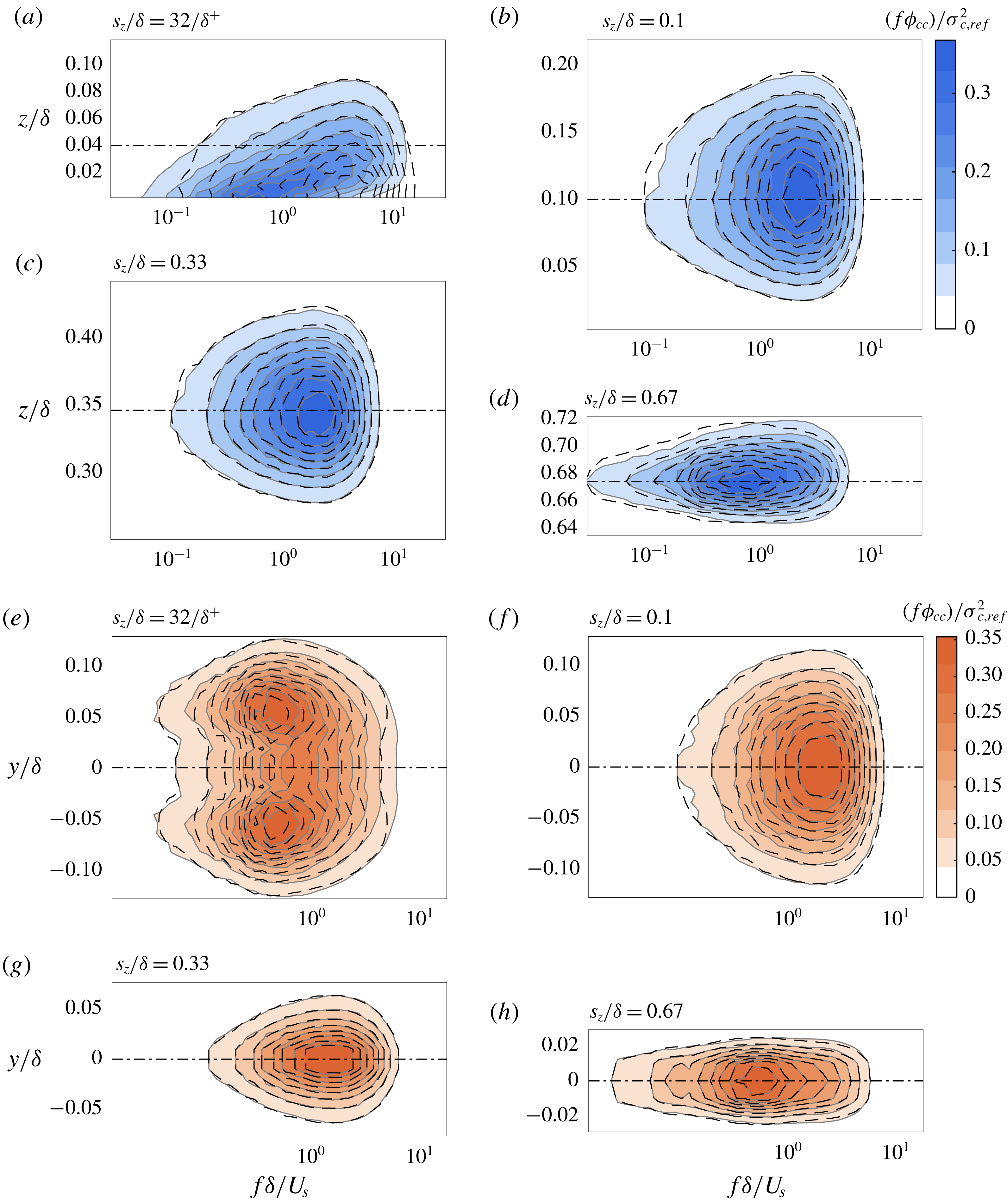
Contour maps of pre-multiplied energy spectra (
 $f\unicode[STIX]{x1D6F7}_{cc}/\unicode[STIX]{x1D70E}_{c,ref}^{2}$
) of concentration fluctuations plotted as a function of
 $f\unicode[STIX]{x1D6FF}/U_{s}$
and (a–d)
 $z/\unicode[STIX]{x1D6FF}$
; (e–h)
 $y/\unicode[STIX]{x1D6FF}$
. Each panel shows concentration spectra for plume released at different source heights. Horizontal dashed lines indicate the source location. Coloured contours and solid-grey lines indicate experimental data; dashed-black lines indicate prediction using (4.3). Eight levels of
 $f\unicode[STIX]{x1D6F7}_{cc}/\unicode[STIX]{x1D70E}_{c,ref}^{2}$
from experiments are indicated, while the dashed-lines represent the prediction at same levels.

4.2 Ground level source
As evident from the discussion on model parameters, the ground level source exhibits different characteristics in comparison to elevated sources, namely the variance distribution and the reference spectrum. Revisiting the results plotted in figures 2(b) and 6(a), it is observed that the ground level plume has two distinct peaks in its variance distribution along
 $y$
. This result is consistent with several past experimental studies on jets and plumes (Becker, Hottel & Williams Reference Becker, Hottel and Williams1967; Birch et al.
Reference Birch, Brown, Dodson and Thomas1978; Fackrell & Robins Reference Fackrell and Robins1982a
; Pitts & Kashiwagi Reference Pitts and Kashiwagi1984). Based on these observations, Chatwin & Sullivan (Reference Chatwin and Sullivan1990) presented a two parameter (
 $\unicode[STIX]{x1D6FC}$
,
 $\unicode[STIX]{x1D6FD}$
) model that predicted the off-axis peak behaviour of
 $\unicode[STIX]{x1D70E}_{c}^{2}(y)$
in the near-field region of a dispersing scalar from a uniform source. Later, Sawford & Sullivan (Reference Sawford and Sullivan1995) developed the model further by taking into account of the source distribution as,
 $$\begin{eqnarray}\displaystyle \unicode[STIX]{x1D70E}_{c}^{2}(y)=\unicode[STIX]{x1D6FD}^{2}C_{0}^{2}\unicode[STIX]{x1D712}(\unicode[STIX]{x1D6FC}-\unicode[STIX]{x1D712}), & & \displaystyle\end{eqnarray}$$
where
 $\unicode[STIX]{x1D712}=C(y)/C_{0}$
and
 $C_{0}$
is the maximum mean concentration on the plume axis. In the model,
 $\unicode[STIX]{x1D6FC}$
is concerned with the evolution of the plume that is controlled by large eddies of the velocity field and hence it depends on source geometry, type of flow and development distance. On the other hand,
 $\unicode[STIX]{x1D6FD}$
accounted for the in-plume dissipation. Using this model, Sawford & Sullivan (Reference Sawford and Sullivan1995) demonstrated that for
 $\unicode[STIX]{x1D6FC}<2$
, there is an off-axis maximum in the variance profile. In the current study, the values of
 $\unicode[STIX]{x1D6FC}=1.3$
and
 $\unicode[STIX]{x1D6FD}=0.78$
are obtained by fitting the variance profile to (4.4) and the fit is shown as a dashed line in figure 2(b).
A second important difference between ground level and elevated sources is the location of the reference spectrum used for predicting spectra across the plume in the vertical direction. In our analysis, it is observed that the concentration spectrum on the plume axis for a ground level source was limited to a smaller bandwidth of frequencies, which is consistent with the behaviour of streamwise velocity spectra in the near-wall region. In order to capture the full bandwidth of frequencies, we chose the geometric mid-point of the log region, i.e.
 $z_{ref}^{+}=\sqrt{(3.6\sqrt{\unicode[STIX]{x1D6FF}^{+}})~(0.2\unicode[STIX]{x1D6FF}^{+})}=0.85{\unicode[STIX]{x1D6FF}^{+}}^{(3/4)}$
(Morrill, Philip & Klewicki Reference Morrill, Philip and Klewicki2017) as the appropriate reference location for a ground level source. With this modification, the model is able to yield better predictions of the concentration spectra across the entire plume (cf. figure 8
a in the following section).
4.3 Spectrum predictions
With the model parameters established, the
 $c$
-spectra can now be predicted at all locations in the plume using (4.2), where the only inputs are a reference
 $f\unicode[STIX]{x1D6F7}_{cc}$
from figure 7(b) and the concentration variance profile, defined using plume half-width in (4.3). We recall that data are collected for eight different
 $s_{z}/\unicode[STIX]{x1D6FF}$
and four
 $s_{x}/\unicode[STIX]{x1D6FF}$
locations; however, for brevity only limited measurements will be discussed here. Figure 8(a–d) shows concentration spectra varying with wall distance for four different source heights as coloured contours, whereas the predicted spectra are indicated by dashed-black lines. Together, these data cover the source heights across the entire boundary layer (buffer region, log region and the outer region). The horizontal dot-dashed line in each panel marks the reference location. Note that the vertical size of each panel proportionally indicates the plume size relative to the TBL thickness. Overall, the predictive model contours agree very well with measurements for all source heights in figure 8(a–d). The principal effect of varying source height, i.e. the frequency shift and location of the peak, is suitably accounted for by the model in figure 8(b–d), whereas, for the ground level source, the peak in the two-dimensional spectrum map is not accurately predicted. The influence of the wall on spectra of concentration very close to the surface requires further investigation.
The model is also tested by comparing the predicted spectra with measurements in the spanwise direction, and these are shown in figure 8(e–h). Again, the predictive model is able to capture the variation of
 $c$
-spectra in the spanwise direction for the plume at four source heights. As highlighted before, the distribution of variance for a ground level source along
 $y$
is not Gaussian (cf. figure 2
a). In this case, the analytical model for concentration variance (see (4.4)) proposed by Sawford & Sullivan (Reference Sawford and Sullivan1995) is used as an input to the model for predicting
 $c$
-spectra. With this refinement, the model is able to accurately represent the two peaks on either side of the plume axis in figure 8(e).
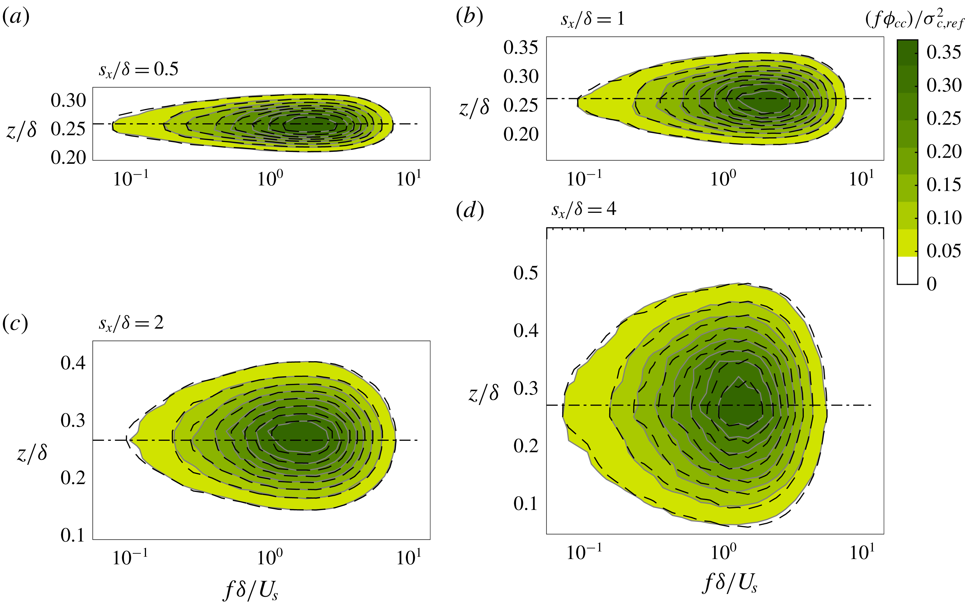
Finally, the model is also employed to predict
 $c$
-spectra at a fixed height but varying source distance
 $s_{x}$
in figure 9(a–d). As a representative case,
 $s_{z}/\unicode[STIX]{x1D6FF}=0.25$
is considered here and prediction results at other source heights are comparable. Note that here the streamwise variation of concentration variation is also needed, i.e. of the form
 $\unicode[STIX]{x1D70E}_{c,ref}^{2}=A(s_{x}/\unicode[STIX]{x1D6FF})^{B}$
. It is found that
 $A=663.5$
and
 $B=-2.25$
in our study, and a similar power law can be readily obtained from plume models or standard experiments (e.g. Nironi et al.
Reference Nironi, Salizzoni, Marro, Mejean, Grosjean and Soulhac2015). Similar to figure 8, the contour maps of measured
 $c$
-spectra in figure 9 are compared against predicted contour lines for four different streamwise locations. There is an excellent agreement between model predictions and the measured values for source distances up to
 $4\unicode[STIX]{x1D6FF}$
. In this representation, it is clearly seen that the plume grows in the streamwise direction and the model works well if the streamwise development of
 $\unicode[STIX]{x1D6FF}_{\unicode[STIX]{x1D70E}}$
is appropriately accounted for.
Same as figure 8. Each panel shows concentration spectra for plumes released at different source distances,
 $s_{x}/\unicode[STIX]{x1D6FF}=0.5$
, 1, 2 and 4, for a log-region source,
 $s_{z}/\unicode[STIX]{x1D6FF}=0.25$
.

5 Discussion
5.1 Non-dimensional analysis of the concentration spectra
In order to ascertain if there exists a scaling behaviour of concentration spectrum, here a heuristic approach via non-dimensional analysis is undertaken. First, it is reasonable to consider that the spatial spectrum of passive scalar concentration
 $E_{cc}(k,x,y,z)$
or the temporal counterpart
 $\unicode[STIX]{x1D6F7}_{cc}(f,x,y,z)$
depends on the plume characteristics as well as background velocity field. For a point-source plume, we consider the plume variance
 $\unicode[STIX]{x1D70E}_{c}^{2}(x,y,z)$
and a characteristic concentration length scale
 $l_{c}(x)$
as appropriate scales based on the analysis of Hanna & Insley (Reference Hanna and Insley1989). For velocity, we consider the local mean velocity
 $U(z)$
, the velocity variance
 $\unicode[STIX]{x1D70E}_{u}^{2}(z)$
and a characteristic velocity length scale
 $l_{u}(z)$
. Thus, one can write,
 $$\begin{eqnarray}\displaystyle E_{cc}=\text{func}(k,\unicode[STIX]{x1D70E}_{c},l_{c},U,\unicode[STIX]{x1D70E}_{u},l_{u}),\quad \text{or}\quad \unicode[STIX]{x1D6F7}_{cc}=\text{func}(f,\unicode[STIX]{x1D70E}_{c},l_{c},U,\unicode[STIX]{x1D70E}_{u},l_{u}). & & \displaystyle\end{eqnarray}$$
Non-dimensional analysis suggests:
 $$\begin{eqnarray}\displaystyle \frac{kE_{cc}}{\unicode[STIX]{x1D70E}_{c}^{2}}=\text{func}\left(kl_{u},\frac{l_{c}}{l_{u}},\frac{\unicode[STIX]{x1D70E}_{u}}{U}\right),\quad \text{or}\quad \frac{f\unicode[STIX]{x1D6F7}_{cc}}{\unicode[STIX]{x1D70E}_{c}^{2}}=\text{func}\left(\frac{fl_{u}}{U},\frac{l_{c}}{l_{u}},\frac{\unicode[STIX]{x1D70E}_{u}}{U}\right). & & \displaystyle\end{eqnarray}$$
There are several features in this functional form that deserve comments:
(i) The non-dimensionalisation of wavenumber or frequency (i.e.
$kl_{u}$
or
$fl_{u}/U$
) is with
$l_{u}$
and not
$l_{c}$
because it was observed in our recent study that concentration fluctuations are passively advected in all directions by the velocity field (Talluru et al.
Reference Talluru, Philip and Chauhan2018). Further, from figure 4 and related discussion, it is clear that
$l_{u}$
is a more appropriate length scale than
$l_{c}$
for normalising
$k$
or
$f$
.(ii) The choice of
$l_{u}$
is not straightforward. There are multiple length scales present in the velocity field of a turbulent boundary layer and they scale differently with Reynolds number. For example, within the log region of a TBL, the larger length scales of the
$u$
-spectrum scale with the boundary layer thickness,
$\unicode[STIX]{x1D6FF}$
(Baidya et al.
Reference Baidya, Philip, Hutchins, Monty and Marusic2017). Likewise, the large scales in the
$v$
- and
$w$
-spectra also scale with
$\unicode[STIX]{x1D6FF}$
(Baidya et al.
Reference Baidya, Philip, Hutchins, Monty and Marusic2017). It is known from previous studies (e.g. Hanna & Insley Reference Hanna and Insley1989; Talluru et al.
Reference Talluru, Philip and Chauhan2018) that the peak ‘energy’ in
$E_{cc}$
or
$\unicode[STIX]{x1D6F7}_{cc}$
is located at a frequency somewhere between the peak energy location of
$u$
and
$v$
or
$w$
, and that meandering is a large-scale phenomenon (Talluru et al.
Reference Talluru, Philip and Chauhan2018), suggesting the suitability of taking
$l_{u}=\unicode[STIX]{x1D6FF}$
for large scales.(iii) There are two choices for
$l_{c}$
, either the width of the mean concentration distribution (
$\unicode[STIX]{x1D6FF}_{C}$
) or the width of variance distribution (
$\unicode[STIX]{x1D6FF}_{\unicode[STIX]{x1D70E}}$
). In the present analysis this is of minimal importance if we consider a narrow plume, i.e. the plume width
$l_{c}$
is small compared to
$\unicode[STIX]{x1D6FF}$
or
$l_{u}$
and it has a weak variation in
$x$
. This is corroborated by our data within our range of experimental parameters. As such, we expect minimal dependence on
$l_{c}/l_{u}$
, and this factor can be ignored from (5.2).(iv) For
$\unicode[STIX]{x1D70E}_{u}$
one could consider any of the variance of
$u$
,
$v$
,
$w$
or the kinetic energy. However, the ratio
$\unicode[STIX]{x1D70E}_{u}/U$
does not vary significantly if the plume width is much smaller than the boundary layer thickness i.e. narrow plume assumption (see figure 7). Furthermore, for our data the ratio is a weak function of
$z$
, and hence ignored from (5.2).


The above points suggest that (5.2) can be simplified to:
 $$\begin{eqnarray}\displaystyle \frac{kE_{cc}}{\unicode[STIX]{x1D70E}_{c}^{2}}=\text{func}(kl_{u}),\quad \text{or}\quad \frac{f\unicode[STIX]{x1D6F7}_{cc}}{\unicode[STIX]{x1D70E}_{c}^{2}}=\text{func}\left(\frac{fl_{u}}{U}\right). & & \displaystyle\end{eqnarray}$$
The validity of this functional form is evident in figure 3(d), where, we have employed the appropriate length and velocity scales
 $l_{u}\mapsto l_{u-int}$
and
 $U\mapsto U_{s}$
.
Note that the second equation in (5.3) also forms the basis of spectrum model in § 4 that is able to predict spectra in very good agreement with experimental data. Now, if we write the second equation in (5.3) for a fixed frequency, say
 $f_{1}$
and two locations (say,
 $y_{1}$
and
 $y_{2}$
and at a fixed
 $z$
), and take a ratio of the two, we obtain,
 $$\begin{eqnarray}\displaystyle \frac{f_{1}\unicode[STIX]{x1D6F7}_{cc}(y_{1})}{\unicode[STIX]{x1D70E}_{c}^{2}(y_{1})}\left/\frac{f_{1}\unicode[STIX]{x1D6F7}_{cc}(y_{2})}{\unicode[STIX]{x1D70E}_{c}^{2}(y_{2})}\right.=\text{func}\left(\frac{f_{1}l_{u}}{U}\right)_{y_{1}}\left/\text{func}\left(\frac{f_{1}l_{u}}{U}\right)_{y_{2}}\right.. & & \displaystyle\end{eqnarray}$$
Evidently the right-hand side of (5.4) is neither a function of
 $y_{1}$
nor
 $y_{2}$
, and the left-hand side shows that it is independent of frequency. Hence the ratio returns to
 $1$
, and we recover the basis for our predictive model (3.1).
5.2 Relation to some other models
A prominent model for spectra is the two time scale spectrum model put forth by Hanna (Reference Hanna1986). The basis of this model is the two dominant time scales present in a narrow meandering plume – (i) time scale of the meandering motions (
 $T_{E}$
) and (ii) the time scale of the small-scale plume motions (
 $T_{c}$
). Hanna (Reference Hanna1986) demonstrated that the concentration spectra can be fitted using a linear combination of two Markov spectra given by
 $$\begin{eqnarray}\displaystyle \frac{f\unicode[STIX]{x1D6F7}_{cc}}{\unicode[STIX]{x1D70E}_{c}^{2}}=\frac{(2/\unicode[STIX]{x03C0})f\,T_{i}}{1+(f\,T_{i})^{2}}, & & \displaystyle\end{eqnarray}$$
where
 $T_{i}$
is the period with peak spectral energy. Here,
 $T_{i}$
is taken as
 $T_{E}$
or
 $T_{c}$
for generating the two Markov spectra. He suggested that the two components of Markov spectra are weighed by
 $\unicode[STIX]{x1D6E4}$
and
 $1-\unicode[STIX]{x1D6E4}$
, where
 $\unicode[STIX]{x1D6E4}$
is the fraction of time when non-zero concentrations occur or there is intermittency. It is easy to see that the large
 $f$
asymptote of (5.5) is
 $f\unicode[STIX]{x1D6F7}_{cc}\propto f^{-1}$
rather than
 $f\unicode[STIX]{x1D6F7}_{cc}\propto f^{-2/3}$
as discussed above based on the theoretical analysis of Panofsky & Dutton (Reference Panofsky and Dutton1984).
Interestingly, Hanna’s equation (5.5) also can reduce to our relation (3.1) if we assume that
 $T_{i}$
is independent of the
 $y$
-location within a plume, which is quite likely for a narrow plume. However, it is certainly unlikely that
 $\unicode[STIX]{x1D6E4}$
is independent of
 $y$
. In fact,
 $\unicode[STIX]{x1D6E4}$
is defined to vary from a maximum at the plume centreline and reduce to zero outside the plume as we traverse in
 $y$
-direction. Note that similar arguments exist for
 $z$
-direction also.
Next, we examine the relation between (5.3) and the inertial regime scaling. To this end, let us replace
 $\unicode[STIX]{x1D70E}_{c}^{2}$
(the total ‘concentration energy’) with the scale-dependent concentration energy or the second-order scalar structure function,
 $\langle \unicode[STIX]{x0394}c\rangle ^{2}(r)$
. Here,
 $r$
is the axial distance over which the concentration difference
 $\unicode[STIX]{x0394}c\equiv c(x+r)-c(x)$
is taken, and therefore
 $r$
is proportional to the inverse of the wavenumber,
 $r\sim 1/k$
. Also, for large
 $r$
, the concentration becomes independent of
 $r$
, such that,
 $\lim _{r\rightarrow \infty }\langle \unicode[STIX]{x0394}c\rangle ^{2}(r)=2\unicode[STIX]{x1D70E}_{c}^{2}$
. Now, in the inertial regime, the spectral energy at a particular wavenumber (
 $kE_{cc}$
) is proportional to the scale-dependent energy
 $\langle \unicode[STIX]{x0394}c\rangle ^{2}$
, and hence (5.3) (assuming
 $\unicode[STIX]{x1D70E}_{c}$
does not change significantly with
 $r$
) can be written as,
 $$\begin{eqnarray}\displaystyle \frac{k\;E_{cc}(1/k)}{\langle \unicode[STIX]{x0394}c\rangle ^{2}(1/k)}=\unicode[STIX]{x1D6FC}~\text{(a constant)}. & & \displaystyle\end{eqnarray}$$
In the inertial regime,
 $\langle \unicode[STIX]{x0394}c\rangle ^{2}(1/k)=\unicode[STIX]{x1D700}_{c}\,\unicode[STIX]{x1D70F}_{c}(k)$
, where
 $\unicode[STIX]{x1D70F}_{c}$
is now the scale-dependent concentration time scale. Since concentration is predominantly driven by the time scales of velocity,
 $\unicode[STIX]{x1D70F}_{c}$
is considered equal to the velocity time scale
 $\unicode[STIX]{x1D70F}_{u}$
, and for homogeneous turbulence, in the inertial regime,
 $\unicode[STIX]{x1D70F}_{u}$
depends only on the energy dissipation
 $\unicode[STIX]{x1D700}_{u}$
and
 $k$
, i.e.
 $\unicode[STIX]{x1D70F}_{u}=\unicode[STIX]{x1D700}_{u}^{-1/3}k^{-2/3}$
(Obukhov Reference Obukhov1949). Substituting these expressions in (5.6) leads to the expected,
 $E_{cc}(k)=\unicode[STIX]{x1D6FC}\unicode[STIX]{x1D700}_{c}\unicode[STIX]{x1D700}_{u}^{-1/3}k^{-5/3}$
. For shear flows, such as ours,
 $\unicode[STIX]{x1D6FC}$
approaches a constant only at very high (Taylor) Reynolds numbers
 $Re_{\unicode[STIX]{x1D706}}$
, of
 $O(1000)$
. In the present boundary layer
 $Re_{\unicode[STIX]{x1D706}}\approx 200{-}300$
, and as such, we do not expect to observe a clear inertial regime scaling of
 $k^{-5/3}$
.
6 Conclusions
Detailed experiments to measure fluctuating concentration along transverse and vertical directions of a point-source plume have enabled us to map spectra and examine their scaling behaviour. Data of
 $\unicode[STIX]{x1D6F7}_{cc}$
provide overwhelming evidence for the self-similarity at all locations within the plume. The observed self-similarity is consistent with the meandering plume behaviour (Gifford Reference Gifford1959) and the influence of large scales in the physical model put forth by Talluru et al. (Reference Talluru, Philip and Chauhan2018); also see Vanderwel & Tavoularis (Reference Vanderwel and Tavoularis2014). Experimental evidence for length and velocity scales reveal that the integral length scale of the streamwise velocity (or equivalently boundary layer thickness (
 $\unicode[STIX]{x1D6FF}$
) in our case) and the source velocity (
 $U_{s}$
) are appropriate normalising scales for frequency, whereas magnitude of spectra should be normalised by local concentration variance. A non-dimensional analysis coupled with known properties of the point-source plumes in TBL also suggests a self-similar concentration spectra (
 $\unicode[STIX]{x1D6F7}_{cc}$
) that is a function of only normalised frequency. Our experimental data as well as the analysis suggest that, at each frequency, the concentration energy is distributed across the vertical and spanwise directions that is proportional to the concentration variance at that location, as represented by (3.1). This self-similarity is extended to provide a predictive model written as (4.1) and (4.2), which can estimate
 $\unicode[STIX]{x1D6F7}_{cc}$
at any position inside a meandering plume given
 $\unicode[STIX]{x1D6F7}_{cc}$
at another position and a concentration variance defined fully by its width. The model is tested for a wide range of source locations and distances, and is found to yield excellent predictions. The proposed method to estimate
 $\unicode[STIX]{x1D6F7}_{cc}$
would be of value for atmospheric boundary layer flows, where detailed measurements of the industrial plumes are difficult as well as limited by existing instrumentation.