Introduction
Phase shifters play a crucial role in the field of radar and wireless communications, especially in the context of phased array antennas [Reference Mailloux1]. This technology requires multiple radiating elements and an electrically controlled phase shifter for each array element to provide beam scanning and shaping. Consequently, increased complexity and cost are introduced into the system, especially when a large number of array elements are required to generate narrow beams [Reference Ivić, Curtis, Forren, Mendoza, Schvartzman, Torres, Wasielewski and Zahrai2].
A frequency scanning antenna array is a special case of phased array antennas wherein beam scanning is achieved by varying carrier frequency of the transmitted signal [Reference Danielsen and Jorgensen3]. This approach, referred to here as frequency-dependent phase shifters, is a cost-effective method because it replaces expensive RF phase shifters with passive devices whose phase response is designed as a function of frequency variations.
There are several proposals for the implementation of these devices. For example, in [Reference Karimkashi, Zhang, Kishk, Bocangel, Kelley, Meier and Palmer4] series connection of array elements with delay lines is used to provide frequency beam scanning. The alternative proposed in [Reference Lv, Cao, Zeng and Shi5] increases the scanning range using surface plasmon polariton structures to enhance the phase difference compared to traditional delay lines. The approach presented in [Reference Fackelmeier and Biebl6] explores the use of band-pass filters to achieve high phase shifting within a narrow frequency range. In [Reference Ren, Choi and Itoh7] the authors propose a two-port feed network comprising series capacitors and shunt inductors for backward-to-forward beam scanning. Although all these proposals have in common the connection of antennas in series, it should be noted that frequency-dependent phase shifters are versatile and can also be applied in parallel-fed configurations, as demonstrated in [Reference Nishio, Xin, Wang and Itoh8]. Despite the abundance of phase shifter fabrication options, the designs are presented only for specific purposes in each case. Only in [Reference Ren, Choi and Itoh7] the analytical expression for modifying the design to meet new requirements is presented. However, this architecture has limitations in high-frequency implementations, due to the use of discrete components whose behavior deviates at high frequencies because of parasitic elements.
In this paper, we propose a novel architecture for the design of a frequency-dependent phase shifter based on open-stubs for microwave and millimeter wave applications. The architecture can be considered for series and parallel fed array antennas. We provide the analytical expression and analysis, demonstrating the versatility of our architecture to generate a desired phase response with low insertion loss over the required frequency range by selecting the number and characteristic impedance of the open-stubs. Although the presented validation prototype focuses on back-to-forward beam-scanning applications in array antennas, the analytical expressions and design can be adapted to any application.
The paper is organized as follows. In Section II the analytical model of the phase shifter is presented and its transfer function is derived. In Section III an architecture is proposed to compare the response of the phase shifter with a conventional transmission line. Then, in Section IV, a fabricated prototype is tested to evaluate its performance in comparison with the theoretical results. Finally, conclusions are presented in Section V.
Problem formulation
The transfer function of a lossless transmission line of length L can be represented by the scattering parameter S 21 which links the output and input signals under matched conditions as
 \begin{equation}
S_{21}^l = e^{-j\beta L},
\end{equation}
where  $-\beta L$ is the phase response of the line, which is a function of the operating frequency through the phase constant β as
 \begin{equation}
\beta = \frac{2\pi f}{v_p},
\end{equation}
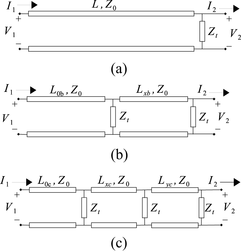
being 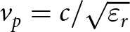 $v_p=c/\sqrt{\varepsilon_r}$ the phase velocity of the electromagnetic field in a board substrate of relative permittivity ɛr and c the speed of light. Note that the phase response is linear and its slope can be designed from the line length and the permittivity of the substrate. While this is an alternative to generate different phases at different frequencies, it has limitations in several applications because these parameters also impact on other characteristics such as size and losses. In this work we propose an architecture based on the connection of open or short stubs that allows designing the phase response of the transmission line (TL) by changing the characteristic impedance of the stubs. To describe the theory, we derive the analytical models of three networks that consists of a conventional TL of characteristic impedance Z 0 and length L connected to (a) one open-stub as shown in Fig. 1a, (b) two open-stubs at a distance Lxb from each other as shown in Fig. 1b, and (c) three open-stubs with distances Lxc and Lyc as shown in Fig. 1c, keeping L always the same. Hence, this implies that L for the last two cases is
 $L=L_{0b}+L_{xb}$ and
 $L=L_{0c}+L_{xc}+L_{yc}$, respectively.
Proposed design of a frequency-controlled phase shifter. TL with (a) one stub, (b) two stubs, and (c) three stubs.

The open-stubs in Fig. 1 are represented by an equivalent lumped-element Zt which models the impedance of each stub on the main transmission line. Note that the architecture of the first network consists of the cascade of two individual components: a transmission line and a stub. On the other hand, the last two networks can be seen as the cascade of two-port networks with the same structure of the first network. For this reason, to simplify the calculation of the analytical models, we use the ABCD matrix [Reference Pozar9] to characterize each network, which relate the input voltage, V 1, and current, I 1, with the output voltage, V 2, and current, I 2, as
 \begin{equation}
\left[\begin{array}{c}
V_1 \\
I_1
\end{array}\right]=\left[\begin{array}{cc}
A & B \\
C & D
\end{array}\right]\left[\begin{array}{c}
V_2 \\
I_2
\end{array}\right],
\end{equation}
and it allows obtaining the S 21 parameter by the following two-port network conversion [Reference Pozar9]
 \begin{equation}
S_{21} = \frac{2}{A+B/Z_0+CZ_0+D},
\end{equation}
for the networks loaded with Z 0. One of the advantages of dealing with ABCD matrices is that the ABCD matrix of the cascade of two-port networks can be found by multiplying the ABCD matrices of the individual two-ports [Reference Pozar9].
Network (a)
For a transmission line of characteristic impedance Z 0 and length L the matrix coefficients are [Reference Pozar9]
 \begin{equation}
\begin{array}{ccc}
A_{l} = \cos{\beta L} & ~~~ & C_{l} = jY_0\sin{\beta L} \\
B_{l} = jZ_0\sin{\beta L} & ~~~ & D_{l} =\cos{\beta L}
\end{array}
\end{equation}
where  $Y_0=1/Z_0$ is the characteristic admittance of the TL. In addition, for the shunt-stub the matrix coefficients are [Reference Pozar9]
 \begin{equation}
\begin{array}{ccc}
A_s = 1 & ~~~ & C_s = 1/Z_t \\
B_s = 0 & ~~~ & D_s = 1
\end{array}
\end{equation}
being Zt the input impedance of an open-stub of length Lt, whose expression is
 \begin{equation}
Z_t = \frac{Z_1}{j\tan{(\beta L_t)}}
\end{equation}
where  $Z_1=kZ_0$ is the characteristic impedance of the stub line, being k the normalized characteristic impedance respect to Z 0.
Then, the ABCD matrix of the network presented in Fig. 1a is obtained by multiplying the ABCD matrices with the elements given in (5) and (6), which results
 \begin{equation}
\left[\begin{array}{cc}
\!\text{cos}(\beta L)\!-\!Z_0Y_1\text{sin}(\beta L)\text{tan}(\beta L_t) & jZ_0\text{sin}(\beta L)\! \\
\!jY_0\text{sin}(\beta L)\!+\!jY_1\text{cos}(\beta L)\text{tan}(\beta L_t) & \text{cos}(\beta L)\!
\end{array}\right],
\end{equation}
where 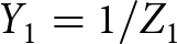 $Y_1=1/Z_1$ and (7) was replaced into the element Cs of (6). Using (4), the S 21 parameter for the first network results
 \begin{equation}
S^a_{21} = \frac{2kS^l_{21}}{2k+j\tan(\beta L_t)}.
\end{equation}
Hence, with this model the magnitude and phase response of S a21 can be designed by selecting the value of k and Lt.
Network (b)
Following an analogous procedure, we can obtain the analytical model of the two-stubs architecture presented in Fig. 1b. In this case, the two-port networks of the cascade connection are of the network (a) type, i.e. a TL followed by a stub. The length of the TL of the first network is  $L_{0b}$ while the length of the TL of the second network is Lxb, and both have characteristic impedance Z 0. The stubs of both networks are considered equal, with length Lt and characteristic impedance Z 1, as described in (7). With this setup the ABCD matrix of each network of the cascade connection has the form of (8) with
 $L_{0b}$ and Lxb instead of L. The product of the resulting ABCD matrices gives the ABCD matrix of the network (b). Then, replacing correspondingly the expression of each matrix element in (4) allows to obtain its S 21 parameter which results
 \begin{equation}
S^b_{21} = \frac{4k^2S^l_{21}}{4k^2\!+\!j4k\!\tan(\beta L_t)\!-\!(1-e^{-j2\beta L_{xb}}\!)\!\tan^2(\beta L_t)}.
\end{equation}
Network (c)
Repeating the procedure described in the previous section with the cascade connection of three two-port networks of the network (a) type it is possible to obtain an expression for the three-stubs architecture presented in Fig. 1c. Considering that the three stubs are equals, i.e. with length Lt and characteristic impedance Z 1, as described in (7), and that the  $L_{0c}$, Lxc and Lyc are the lengths of the three transmission lines, respectively, then the ABCD matrix of each network of the cascade connection has the form of (8) with
 $L_{0c}$, Lxc and Lyc instead of L. The product of the three ABCD matrices gives the ABCD matrix of the network (c) and using the two-port network conversion (4) we obtain the following expression for the S 21 parameter
 \begin{equation}
S^c_{21} = \frac{8k^3S^l_{21}}{\sum_{n=0}^{3} j^n(2k)^{3-n}\xi_n\tan^n(\beta L_t)},
\end{equation}
where
 \begin{align*}
\xi_0 & = 1 \nonumber\\
\xi_1 & = 3 \nonumber\\
\xi_2 & = 3\!-\!e^{-j2\beta L_{xc}}\!-\!e^{-j2\beta L_{yc}}\!-\!e^{-j2\beta (L_{xc}+L_{yc})} \nonumber\\
\xi_3 & = 1\!-\!e^{-j2\beta L_{xc}}\!-\!e^{-j2\beta L_{yc}}\!+\!e^{-j2\beta (L_{xc}+L_{yc})}.\nonumber
\end{align*}
Theoretical results
As an application example, a frequency scanning feed network for a phase array is designed based on the phase and magnitude responses of the S 21 networks parameter derived in previous sections. In order to produce left and right beam scanning, the phase difference between the array elements must be zero at a center frequency, and maximum positive or negative at the minimum or maximum frequencies, respectively. From models (9), (10), and (11) it is possible to achieve zero phase difference between the S 21 of any network and S l21 by selecting Lt to be half a wavelength at the center frequency, f 0, of the frequency range and then, k is set to achieve the desired phase difference at the minimum and maximum frequencies of the range.
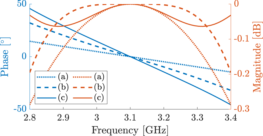
Figure 2 shows the magnitude and phase response of the coefficients S 21 respect to S l21 for the three networks presented in previous sections, where Lt has been set as half a wavelength of the frequency  $f_0=3.1$ GHz and three values of k have been considered: 0.4, 0.6, 1.2. Figure 2a corresponds to the magnitude and phase responses of the ratio
 $S^a_{21}/S^l_{21}$ i.e. for network (a). With this network the phase difference can be increased by choosing a lower k value, at the cost of also increasing the insertion loss. One way to obtain a great phase shift and improve the magnitude response consist in using two or more stubs as used in networks (b) and (c), which achieve a better insertion loss by adjusting the distance between stubs. This behavior can be seen in Figs. 2b and 2c where are presented the magnitude and phase of the ratio
 $S^b_{21}/S^l_{21}$ and
 $S^c_{21}/S^l_{21}$. Comparing the results with those of network (a), the maximum phase difference increases proportionally to the number of open-stubs. Figure 3 further highlights this trend for k = 0.6, showing that the maximum phase difference is approximately 15∘ for network (a) while it is approximately 30∘ and 45∘ for networks (b) and (c), respectively. In addition, the magnitude response of networks (b) and (c) presents variations below 0.1 dB for a frequency range larger than its of the network (a). The distances between stubs of networks (b) and (c) were selected to minimize the insertion losses in the frequency range.
Analytical results of the coefficient S 21 respect to S l21. TL with (a) one stub, (b) two stubs, (c) three stubs.

Coefficient S 21 values respect to S l21 of the three networks for k = 0.6.

Proposed architecture
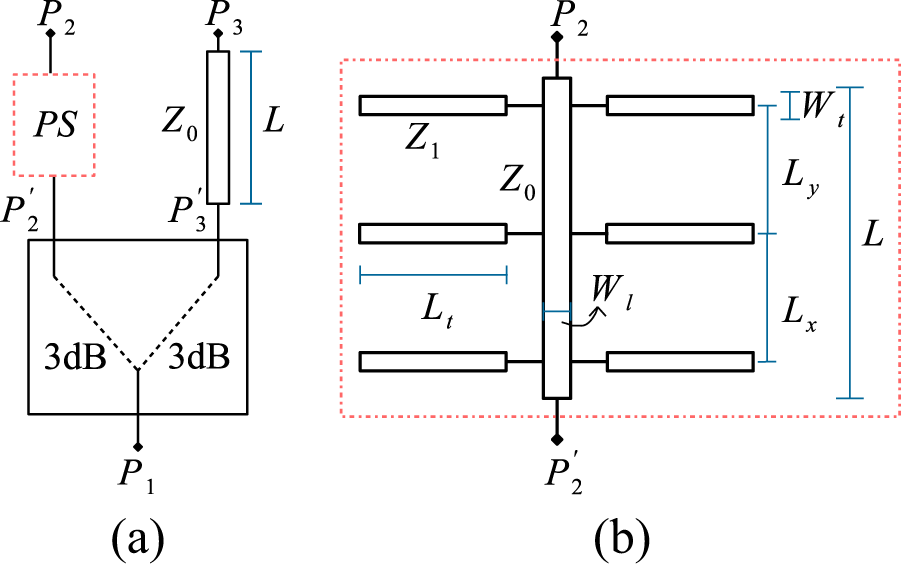
We propose an architecture to validate the frequency-dependent phase shifter model presented in Section II. It consists of a three-port device with an input port P 1 and two output ports P 2 and P 3 as shown in Fig. 4(a). The architecture is based on a wide-band power divider whose input is the port P 1, one of its outputs, denoted  $P_2'$, is connected to the proposed Phase Shifter (PS), while the other output port, denoted
 $P_3'$, is connected to a conventional TL of length L and characteristic impedance Z 0. Neglecting the magnitude and phase imbalance of the power divider, the scattering coefficient S 31 corresponds to S l21, while the scattering coefficient S 21 represents S i21 where i is a, b or c, depending on the network used as PS. Then, the ratio of the scattering parameters S 21 and S 31 of the three-port architecture is used to validate the theoretical model presented in Section II because in these conditions it is equal to the ratio
 $S^i_{21}/S^l_{21}$ with
 $i\in\{a,b,c\}$.
Scheme of the proposed architecture of (a) the three port prototype, and (b) the phase shifter.

The architecture is designed to operate in the 2.8 GHz to 3.4 GHz frequency range, with a central frequency of 3.1 GHz. The details of the design of each block of the circuit are presented below.
Wide-band power divider
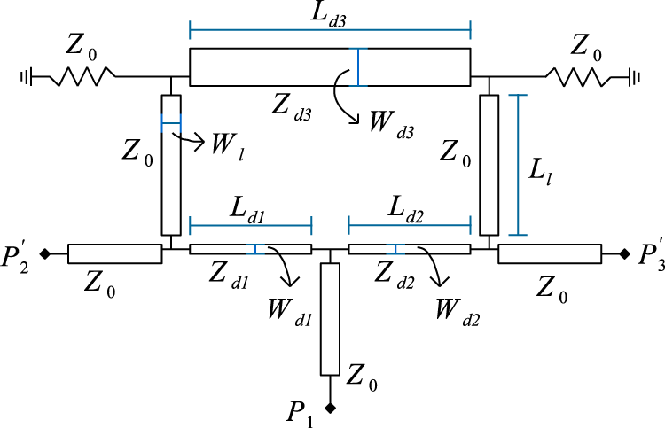
The phase shifter is connected to a conventional Gysel power divider [Reference Ooi, Palei and Leong10] which provides flat amplitude response between the input port P 1 and the output ports  $P'_2$ and
 $P'_3$ in the operating frequency range. The schematic of the Gysel power divider is shown in Fig. 5.
Schematic of the Gysel power divider.

The design at the center frequency f 0 consists of four  $\lambda_0/4$ lines,
 $L_{d1}$,
 $L_{d2}$, and both Ll, and one
 $\lambda_0/2$ line,
 $L_{d3}$, connected to two Z 0 lumped impedances. The characteristic impedances of the lines are:
 $Z_{d1}=Z_{d2}=\sqrt{2}Z_0$ and
 $Z_{d3}=Z_0/\sqrt{2}$.
Phase shifter
For concept validation, we choose the three-stub Network (c) as the phase shifter, which is shown in Fig. 4(b) and whose theoretical model is described in Section II.C. The length of the line connected between ports  $P'_2$ and P 2 is L, with characteristic impedance Z 0, and the length of the open-stubs are half a wavelength at the center frequency 3.1 GHz to present zero phase difference with respect to the conventional TL of length L at this frequency. In addition, we want to achieve the phase response presented in Fig. 2c for the normalized impedance of the open-stubs with k = 0.6. For microstrip implementation a stub of characteristic impedance
 $Z_1=kZ_0=30\Omega$ is very thick and, therefore to simplify the implementation, we replace it with two k = 1.2 open-stubs in parallel that are thinner and behave the same as one k = 0.6 open-stub. Finally, the distances Lx and Ly between the stubs are selected to minimize the insertion loss of the phase shifter in the frequency range, their values are equal and close to a quarter wavelength at the center frequency.
Manufactured prototype
We fabricated the proposed architecture on a RO3010 substrate of Rogers Corporations of relative permittivity 11.2 and thickness 1.27 mm. Figure 6 shows a photography of the manufactured prototype. It has an edge mount SMA connector at each of its three ports and the Gysel power divider has two 50 Ω resistors connected to the ground plane through vias. All relevant dimensions of the prototype are depicted in Table 1 and were obtained from standard microstrip equations [Reference Pozar9], and subsequently verified through numerical simulation.
Photography of the prototype manufactured at 3.1 GHz

Dimensions of the circuit

Experimental results
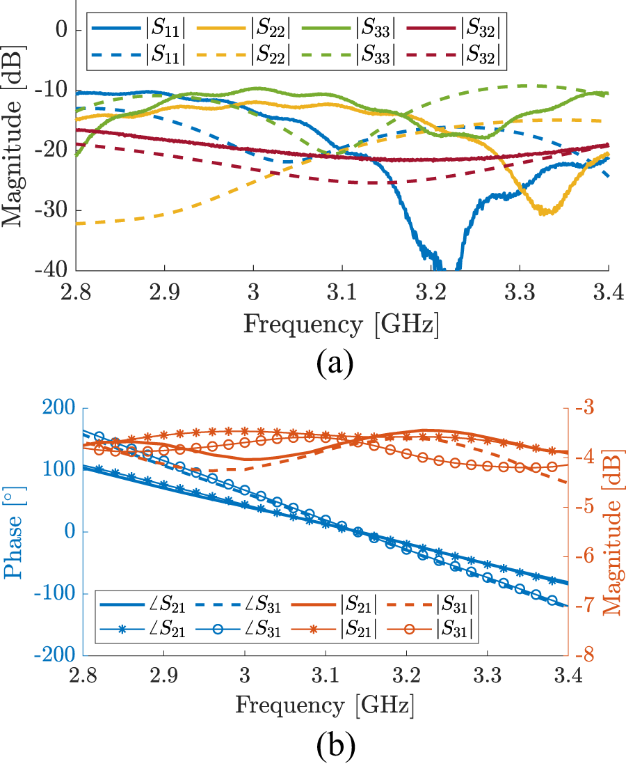
We measured the scattering parameters of the manufactured prototype in the frequency range of 2.8 GHz to 3.4 GHz, using a network analyzer N9918A from Keysight. Figure 7(a) shows the magnitude of scattering parameters S 11, S 22, S 33 and S 32 and Fig. 7(b) the magnitude and phase of the parameters S 21 and S 31. For all measurements the output power of the network analyzer was set in −15 dBm.
Results of the S-parameters of the three port device. (a) Magnitude of parameters S 11, S 22, S 33, and S 32, and (b) magnitude and phase of parameters S 21 and S 31. Measured results are indicated at the top of the legend, and simulated results at the bottom.

Note that the magnitude of the coefficients S 11, S 22, and S 33 are below -10 dB in the entire frequency range, i.e. the 10 dB input return losses criteria are achieved in the operating frequency range, which implies that the network is matched. Additionally, the magnitude of S 32 is below −18 dB which leads a high isolation and the magnitude of the coefficients S 21 and S 31 show that the insertion loss is 3.6 dB, bounded with an amplitude error of 0.6 dB. These insertion loss values are expected, because the prototype has a power divider at the input which implies at least a 3 dB of insertion loss.
On the other hand, the phases responses of the coefficients S 21 and S 31 have a linear behavior and they have the same value at the frequency 3.15 GHz close to the 3.1 GHz specified in the requirements. An error of  $1.6\%$ is acceptable for a prototype and the difference may even be due to dielectric permittivity discrepancy with respect to its nominal value.
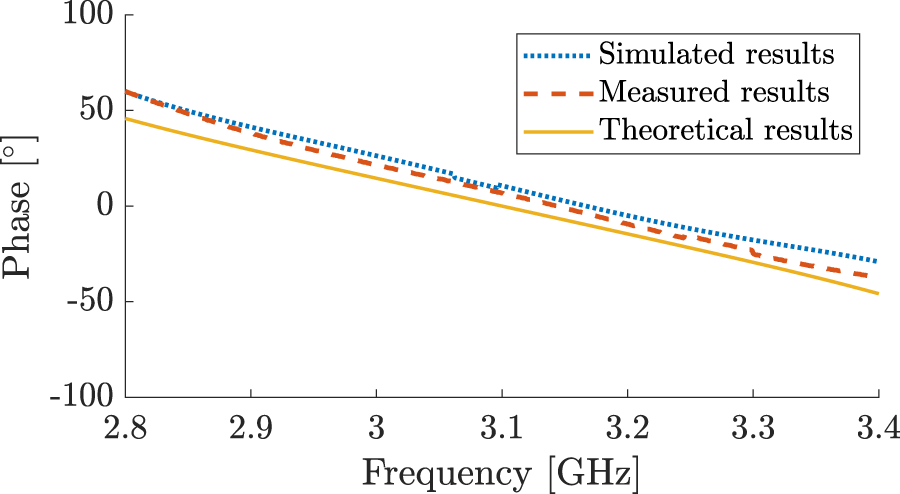
To validate the theory presented in Section II.D, in Fig. 8 we compare the phase of the ratio  $S_{31}/S_{21}$ of measured coefficients, with the phase of the ratio
 $S^c_{21}/S^l_{21}$ evaluated with the theoretical relation given by (11). It is also included the phase of the same coefficients ratio obtained by means of numerical simulations. The measured results show a great agreement with the theoretical results, both phases have a linear behavior with the same slope and an offset up to 10 degrees.
Phase of the coefficients ratio  $S_{31}/S_{21}$, i.e., the phase difference
 $\angle{S_{31}}-\angle{S_{21}}$.

Discussion
As shown in Figs. 7 and 8, the results confirm the theoretical model presented in (11). With k = 0.6 and three open stubs, a phase difference of 100∘ is achieved over the entire frequency range, 0.6 GHz, corresponding to a phase variation coefficient of  $h=166^{\circ}/$GHz. Similarly, using k = 0.4, which corresponds to wider open stubs, a coefficient of
 $233^{\circ}/$GHz is obtained without compromising insertion loss. For greater phase variation while maintaining bandwidth, a fourth stub can be added. However, this increases the device size along the main transmission line. In summary, increasing the number of stubs enhances phase variation but also leads to a larger device size. It is worth mentioning that a larger phase coefficient is not necessarily better, as it depends on the specific application needs.
Table 2 compares the bandwidth (BW), device size, and the phase variation coefficient, h, across different studies described in the Introduction.
Characteristics of different frequency-dependent phase shifters.

Most of the characteristics presented in the table were indirectly derived from the properties of frequency-scanning array antennas presented in each work. For instance, the phase difference coefficient as a function of frequency for each device was calculated based on the variation in the maximum peak angle of the radiation pattern and the known distance between antennas. Additionally, the dimensions listed in the table account only for the size of the phase shifters, excluding the rest of the signal distribution circuit. These dimensions are specified relative to the highest wavelength in free space, λmax, corresponding to the minimum frequency of each range. It is not possible to compare the insertion loss of each device, due to insufficient data available to compute it.
Taking as comparison measures the size of the device, the operating frequency range and the phase shift, it is important to remark that our network for the used value of k presents a higher h parameter value than compact size devices proposed in [Reference Karimkashi, Zhang, Kishk, Bocangel, Kelley, Meier and Palmer4] and [Reference Lv, Cao, Zeng and Shi5], its size is significantly more compact than devices presented in [Reference Karimkashi, Zhang, Kishk, Bocangel, Kelley, Meier and Palmer4], [Reference Lv, Cao, Zeng and Shi5] and [Reference Fackelmeier and Biebl6], and, finally, our network is suitable for high-frequency applications, where the behavior of discrete components, such as those used in [Reference Ren, Choi and Itoh7], becomes increasingly challenging to model and predict. Additionally, note that the proposed network offers the possibility of increasing h by reducing the value of k without affecting its size or operating frequency.
Conclusion
A design of a frequency-dependent phase shifter for microwave frequency applications has been presented. The architecture consists of a cascade connection of open-stubs on a transmission line of length L and characteristic impedance Z 0. First of all, analytical model of the device transfer function has been derived and it has been compared with the model of a conventional transmission line of the same length L and impedance Z 0, showing that the phase difference is a linear function whose slope and offset can be configured by setting the length and characteristic impedance of the stubs. Furthermore, the analytical model has shown that the higher the number of stubs and the lower their characteristic impedance, the greater the slope achieved and therefore the greater the phase difference obtained. It is also worth noting that the inclusion of more than one stub has allowed the magnitude of the frequency response to be tuned by selecting their relative positions.
As an application example for back-to-forward beam scanning capability for phased array antennas, a prototype has been implemented in microstrip technology to operate in the frequency range from 2.8 GHz to 3.4 GHz. The measurement results have shown good agreement with the theoretical predictions, observing that zero phase difference between the device and the conventional transmission line is achieved approximately at the center frequency 3.1 GHz and a phase difference up to 50 degrees at the edges of the frequency range.
Acknowledgements
This work was supported in part by the Universidad Nacional de Cuyo under Grant C019-T1 2118/22, and in part by the Universidad Nacional de Río Negro under Grant PI 40-B-1159.
Competing Interests
The authors report no conflict of interest.

Alejandro J. Venere received the Engineering degree and the doctorate degree in electrical engineering from the National University of La Plata, La Plata, Argentina, in 2013 and 2019, respectively. He is currently a Researcher of the Comisión Nacional de Energia Atómica of Argentina and a Professor with the Instituto Balseiro, Argentina. His current research interests include antenna and RF design for wireless applications and agriculture technology.

Juan P. Pascual received his Eng. (2006) and Ph.D. (2014) degrees at the Universidad Nacional de La Plata (UNLP), Argentina. He worked in the design and FPGA implementation of control strategies for Electric Arc Furnaces in Tenaris (2008-2010). His postdoctoral experience include a research visit to the Instituto Balseiro in Bariloche (2015). He is currently a Professor at the Instituto Balseiro, a Researcher at the CONICET and a Researcher at the CNEA, Argentina. His research interests focus on statistical signal processing in radar, digital communication and agriculture technology.

Jorge Cogo received his Engeneering degree (2008) and Master’s degree (2016) from the Universidad Nacional de La Plata (UNLP), Argentina. He worked on the design and implementation of GNSS receivers for space applications, mainly as a software engineer (2008-2017). He is currently a professor and researcher at the Universidad Nacional de Río Negro. His research interests focus on statistical signal processing in radar, digital communications, GNSS and agriculture technology.