



1. Introduction
Natural convection in a fluid-saturated porous medium is a research topic of great interest because of its large variety of uses in the fields of science and engineering, such as groundwater circulation (Diersch & Kolditz Reference Diersch and Kolditz2002), paper manufacturing (Koponen et al. Reference Koponen, Kandhai, Hellen, Alava, Hoekstra, Kataja, Niskanen, Sloot and Timonen1998), geothermal science (Wooding Reference Wooding1976) and underground rock formation (Wen-Jeng & Chi-Feng Reference Wen-Jeng and Chi-Feng1993), etc.
Horton & Rogers Jr (Reference Horton and Rogers1945) and Lapwood (Reference Lapwood1948) conducted the first study to investigate the linear instability analysis of the convection of fluid through horizontal porous media due to vertical thermal gradients that are heated from below. Later, several extensions were made to this physical set-up under different circumstances (see Barletta & Rees Reference Barletta and Rees2012; Deepika & Narayana Reference Deepika and Narayana2015; Kumar et al. Reference Kumar, Narayana and Sahu2020). All these investigations depend on Darcy’s law, which ignores the influence of inertial motion and solid boundaries. Darcy’s law applies to situations where fluid flow is sufficiently slow and in low-porosity porous media. However, when considering the boundary-layer influences near a boundary and the inertial terms that become applicable at high flow velocities, an extended Darcy’s law must be adopted. In cases with large porosity, it may be suitable to employ the Brinkman model (Brinkman Reference Brinkman1949). The Forchheimer model (Forchheimer Reference Forchheimer1901) is used when fluid motion is sufficiently high so that inertial effects cannot be neglected. To include the inertial effects, the velocity term must be added to the momentum equation. Forchheimer (Forchheimer Reference Forchheimer1901) incorporated the square velocity term in the momentum equation. This term was known as the `Forchheimer’s term’ in the analysis of Muskat (Reference Muskat1938). Some of the studies involving the Forchheimer model have been published in the literature (Seddeek Reference Seddeek2006; Barletta et al. Reference Barletta, Celli and Rees2009; Hayat et al. Reference Hayat, Muhammad, Al-Mezal and Liao2016; Mourya et al. Reference Mourya, Kumar and Narayana2024).
It is well known that the physical properties of fluids can vary significantly with temperature, particularly for fluid viscosity. The rise in temperature enhances the transfer process by lessening the viscosity in the momentum boundary layer, thereby affecting the heat transfer rate. As a result, to forecast the flow and heat transfer rate, it is essential to consider viscosity as a function of temperature. For lubricating fluids, the heat produced by internal friction and the corresponding temperature increase result in changes in viscosity, meaning that the assumption of constant viscosity no longer holds. Torrance & Turcotte (Reference Torrance and Turcotte1971) noted that the viscosity of fluids decreases as the temperature increases, whereas gases exhibit the opposite pattern. Subsequently, Weast (Reference Weast1986) provided several tables detailing viscosity values at different temperatures. They observed that even a minor fluctuation in temperature by a few degrees could lead to significant changes in viscosity. After that, several researchers investigated the impact of the temperature dependence of viscosity on convective flow (Yang & Leu Reference Yang and Leu1992; Barletta & Nield Reference Barletta and Nield2012; Shankar et al. Reference Shankar, Nagamani and Shivakumara2023). Harfash & Hameed (Reference Harfash and Hameed2021) studied the stability theory of double diffusion convection in a medium with temperature-dependent viscosity, which varies linearly using the Brinkman–Forchheimer model. They found that the viscosity parameter has a stabilising effect on the system.
Many of the studies in the above-mentioned literature concerned convective motion in isotropic media. However, in many real-life situations, porous media demonstrate anisotropy in their mechanical and thermal characteristics. Anisotropy often arises from the preferred alignment or irregular structure of grains or fibres. A common practical example of such a system is loft insulation, which generally demonstrates less permeability in the insulating layer relative to the perpendicular orientation. Another common example is groundwater flow in anisotropic sedimentary and rock formations. Anisotropy significantly affects fluid flow behaviour and the stability of the system. Anisotropic thermal conductivity or diffusivity occurs when a material’s ability to conduct heat is directionally dependent due to its composition, microstructure or highly asymmetric crystallographic structure. Castinel & Combarnous (Reference Castinel and Combarnous1974) conducted the first study to investigate the linear stability analysis of convective flow in a horizontal porous medium that has anisotropic permeability. This work was extended by Epherre (Reference Epherre1975) taking into account the inclusion of a porous medium exhibiting anisotropic thermal diffusivity. Tyvand & Storesletten (Reference Tyvand and Storesletten1991) and Storesletten (Reference Storesletten1993) addressed anisotropic permeability and thermal diffusivity, respectively, with longitudinal axes that were oblique with respect to the vertical axes. Subsequently, Degan et al. (Reference Degan, Vasseur and Bilgen1995) investigated anisotropic permeability and conductivity in porous media with arbitrary orientation. It was found that the heat transfer was highest when the principal axis with the greatest permeability was parallel to the vertical direction and lowest when perpendicular to the vertical direction. Recently, Mourya et al. (Reference Mourya, Kumar and Narayana2024) examined thermal convection in Darcy–Forchheimer flow within horizontal porous media with thermal anisotropy. They observed that the system exhibited greater stability when the horizontal thermal diffusivity component predominated over the vertical ones. Very recently, Mourya & Kumar (Reference Mourya and Kumar2024) examined the thermal convection in an inclined Darcy–Brinkman porous medium with thermal anisotropy. They also discovered that the system maintains stability and delays the onset of convection when the horizontal components of thermal diffusivity dominate.
Natural convection in porous media driven by an internal heat source has recently attracted significant interest due to its several relevancies in geophysics and energy-related problems. If the fluid is heated internally by a uniform spreading of heat sources, a thermal instability occurs, just as radioactive decay occurs in the Earth’s mantle. Tritton & Zarraga (Reference Tritton and Zarraga1967) and Schwiderski & Schwab (Reference Schwiderski and Schwab1971) conducted experimental studies and discovered several significant features, among them the expansion of convection cells as the rate of internal heat production increased. Subsequently, numerous researchers conducted various investigations of convection problems by incorporating internal heat sources. Some of them are given in Parthiban & Patil (Reference Parthiban and Patil1997), Alex & Patil (Reference Alex and Patil2002), Barletta et al. (Reference Barletta, Celli and Nield2014) and Harfash (Reference Harfash2014). Recently, Deepika et al. (Reference Deepika, Narayana and Hill2017) and Bhadauria et al. (Reference Bhadauria, Kumar, Kumar, Sacheti and Chandran2011) examined the effects of internal heat generation on isotropic and anisotropic porous media, respectively. After studying all the above literature, it is found that the stability region of a fluid layer is reduced when an internal heat source is introduced.
Considering a perfectly horizontal porous medium is generally not physically realistic, as inclinations may occur in practical scenarios. For example, in carbon sequestration, saline aquifers are commonly tilted at an angle to the horizontal (Tsai et al. Reference Tsai, Riesling and Stone2013; Akhbari & Hesse Reference Akhbari and Hesse2017). The inclined porous layer problem was first discovered by Bories & Combarnous (Reference Bories and Combarnous1973) and later further expanded by Weber (Reference Weber1975) and Caltagirone & Bories (Reference Caltagirone and Bories1985). In their work, the authors considered different boundary temperatures and established that instability arises when the Rayleigh number exceeds
 $4\pi ^2/cos\phi$
, where
 $\phi$
is the inclination angle relative to the horizontal. Subsequently, Barletta & Rees (Reference Barletta and Rees2012) investigated a thermal stability analysis on the Darcy–Hadley flow within a tilted porous channel. They found that increasing the channel’s inclination angle led to instability when the upper wall was colder than the lower wall and, conversely, enhanced stability when the upper wall was warmer than the lower wall. Subsequently, Barletta et al. (Reference Barletta, Celli and Nield2014) studied the impact of a uniform internal heat source on the onset of convection in a tilted porous layer, with the upper wall maintained at isothermal conditions and the lower wall being at isothermal or adiabatic conditions. Very recently, Mourya & Kumar (Reference Mourya and Kumar2024) studied the convection problem in Brinkman flow in an inclined porous layer. They observed that increasing the inclination angles led to higher critical values, suggesting a delay in convective motion.
One of the key aspects of the present analysis is the inclusion of temperature-dependent viscosity. This is particularly the case for the fluids, such as oil, whose physical qualities change with temperature. The influences of variable viscosity on convective problems with an internal heat source are discussed by Mourya et al. (Reference Mourya, Kumar and Narayana2024), where the momentum equation is described by the Darcy–Forchheimer momentum equation within the context of isothermal boundaries. However, in many practical situations, thermal boundary conditions are inherently asymmetric (Barletta et al. Reference Barletta, Rossi di Schio and Celli2011, Reference Barletta, Celli and Nield2014). These conditions are commonly observed in geothermal systems and thermal energy storage engineering, where the interaction between fluid rheology and boundary-driven heat transfer dictates the formation of convection and advancement of convective motion. Motivated by this, the present study focuses on the effects of the adiabatic bottom boundary and the isothermal top boundary in an inclined porous media, particularly in the presence of anisotropic thermal diffusivity, temperature-dependent viscosity and internal heat sources. The novelty of the present problem is therefore to investigate the effects of anisotropic thermal diffusivity, temperature-dependent viscosity and internal heat generation on convective motion in an inclined porous medium, using the Darcy–Forchheimer momentum equation, which extends Darcy’s law by incorporating an additional term to account for inertial effects at higher flow velocities. The bottom boundary is assumed to be adiabatic, and the top boundary is considered isothermal. In these situations, the lower boundary temperature exceeds the recommended upper boundary temperature. As there is no externally imposed temperature difference, but rather the heat is generated internally by the action of an internal heat source. This provided the first instances of the combined influences of these factors on the stability properties of thermal convection. The governing set of nonlinear partial differential equations is converted into a system of linear ordinary differential equations through linear stability and normal mode procedures. The resulting generalised eigenvalue problem is further addressed by using the Chebyshev tau-QZ algorithm in MATLAB to determine the critical conditions for convective instability.
2. Mathematical formulation
A schematic diagram depicts the inclined porous media. Arrows denote variable magnitudes and directions of thermal diffusivity.

The system considered consists of an infinitely large fluid saturated porous medium with a thickness
 $d$
inclined at an angle
 $\phi$
to the horizontal. Let us introduce the Cartesian coordinate system
 $(x,y,z)$
, where the lower boundary is located at
 $z = 0$
, and the
 $z$
axis is directed vertically upward, with the vertically downward gravity force
 $\boldsymbol {g} =- g\hat {e_z}$
acting. The bottom boundary
 $z = 0$
is thermally insulated (adiabatic), while the top boundary
 $z = d$
is maintained at a uniform temperature
 $T_{0}$
. The physical configuration of the problem geometry is seen in figure 1. The Boussinesq approximation is employed, assuming that the temperature gradient is small and the variation in the density,
 $\rho$
, is small enough to be neglected everywhere except the gravitational body force components of the momentum equation, giving a linear equation of motion
 \begin{equation} \rho = \rho _{0} (1-\alpha (T-T_{0})), \end{equation}
where the reference density,
 $\rho _{0}$
, is associated with a properly defined reference temperature,
 $T_{0}$
, and
 $\alpha$
represents the thermal expansion coefficient at constant pressure. Moreover, the viscosity of the fluid layer is a function of temperature, which can significantly impact the movement of fluid flow. This study considers a linear fluctuation of viscosity with temperature as described by Palm (Reference Palm1960), Straughan (Reference Straughan2002) and Mourya et al. (Reference Mourya, Kumar and Narayana2024) and is given by
 \begin{equation} \mu (T) = \mu _{0} (1-\gamma (T-T_{0})), \end{equation}
here,
 $\gamma$
represents a positive constant and
 $\mu _{0}$
is the viscosity of the fluid at the reference temperature
 $T_0$
.
The Darcy–Forchheimer model is employed for the momentum equation that involves inertial effects given by
 \begin{equation} \boldsymbol{\nabla }\!P = \frac {-\mu (T) \boldsymbol {V}}{K} - \frac {c \rho _{0}}{\sqrt {K}} \boldsymbol {V} |\boldsymbol {V}|- \rho g \,({\rm sin}\phi \hat {i} +{\rm cos}\phi \hat {k}), \end{equation}
where
 $K$
and
 $P$
are the permeability and pressure of the medium, respectively. The Forchheimer coefficient
 $c$
is commonly referred to as the drag constant, and depends on the medium’s geometry, but remains independent of the fluid’s properties.
The governing continuity, Darcy–Forchheimer momentum (after incorporating (2.1) and (2.2) into (2.3)), and the energy equations are, respectively, as follows:
 \begin{equation} \boldsymbol{\nabla }\boldsymbol{\cdot }\boldsymbol {V} = 0, \end{equation}
 \begin{equation} \boldsymbol{\nabla }\!P = -\frac {\mu _{0}}{K}(1-\gamma (T-T_{0})) \boldsymbol {V} - \frac {c \rho _{0}}{\sqrt {K}} \boldsymbol {V} |\boldsymbol {V}|- \rho _{0} g (1-\alpha (T-T_{0})) ({\rm sin}\phi \hat {i} + {\rm cos}\phi \hat {k}), \end{equation}
 \begin{equation} \frac {1}{M} \frac {\partial T}{\partial t} + \boldsymbol {V}\boldsymbol{\cdot }\boldsymbol{\nabla }T = k_h {\nabla} ^2_{1} T + k_{v} \frac {\partial ^2 T}{\partial z^2} +Q^*, \end{equation}
where
V
= (U, V, W) denotes the velocity and
 $M$
denotes the ratio of heat capacities. The coefficient
 $k_{h}$
is the horizontal thermal diffusivity in the
 $x$
and
 $y$
directions, and
 $k_{v}$
is the vertical thermal diffusivity in the
 $z$
direction. The term
 $Q^*$
is given as
 $Q^*\equiv {Q_{\textit{int}}}/{(\rho _{0} c_{p})_{f}}$
, where
 $Q_{\textit{int}}$
is the volumetric rate of heat generation inside the porous medium,
 $c_p$
is the specific heat capacity at constant fluid pressure and the subscript
 $f$
denotes the fluid. Furthermore,
 ${\nabla} ^2_{1} = {\partial ^2}/{\partial x^2} + {\partial ^2}/{\partial y^2}$
represents the two-dimensional Laplacian operator.
The boundary conditions are (by following Barletta et al. Reference Barletta, Rossi di Schio and Celli2011) defined as follows:
 \begin{equation} \begin{aligned} z = 0, \quad W= 0, \quad \frac {\partial T}{\partial z} = 0,\\ z = d, \quad W= 0, \quad T = T_{0}. \end{aligned} \end{equation}
2.1. Basic steady-state solution
A stationary solution of (2.4)–(2.7) exists corresponding to a purely conductive quiescent state (Lyubimova et al. Reference Lyubimova, Muratov and Shubenkov2022; Rasool Reference Rasool2025) with variations solely dependent on the spatial coordinate
 $z$
. Then, the corresponding base-state velocity and temperature are given as follows:
 \begin{equation} \boldsymbol{V}_{\!B}=0, \quad T_{B}(z)=T_{0} -\frac {Q^{*}d^{2}}{2k_{v}} \left [\left (\frac {z}{d}\right )^{2}-1\right ]\!, \end{equation}
where the subscript
 $B$
indicates the basic state.
2.2. Linear perturbation
To examine the stability of the steady state, we introduce the perturbations
 $(\boldsymbol {U}, \theta , \varPi )$
to the steady-state solutions
 $(\boldsymbol{V}_{\!B}, T_{B}, P_{B})$
in the form of
 \begin{equation} \boldsymbol {V} = \boldsymbol{V}_{\!B}+ \boldsymbol {U},\, T= T_{B} + \theta ,\,P = P_{B} +\varPi , \end{equation}
employing the above perturbations in (2.4)–(2.7) to obtain the following perturbation equation:
 \begin{equation} \boldsymbol{\nabla }\boldsymbol{\cdot }\boldsymbol {U} = 0, \end{equation}
 \begin{equation} \boldsymbol{\nabla }\varPi = - \frac {\mu _{0}}{K} \left \{ 1+ \frac {\gamma Q^* d^2}{2 k_{v}} \left [ \left (\frac {z}{d} \right )^2 -1 \right ] \right \} \boldsymbol {U} + \frac {\mu _{0} \gamma \theta \boldsymbol {U}}{K} - \frac {c \rho _{0}}{\sqrt {K}} \boldsymbol {U} |\boldsymbol {U}| + \alpha g \rho _{0} \theta (\sin \phi \hat {i} + \cos \phi \hat {k}), \end{equation}
 \begin{equation} \frac {1}{M} \frac {\partial \theta }{\partial t} + \boldsymbol {U}\boldsymbol{\cdot }\boldsymbol{\nabla }\theta - \frac {zWQ^*}{k_{v}} = k_{h} {\nabla} ^2_{1} \theta + k_{v} \frac {\partial ^2 \theta }{\partial z^2}, \end{equation}
 \begin{equation} \begin{aligned} z=0, \quad W = 0, \quad \frac {\partial \theta }{\partial z} =0,\\ z=d, \quad W = 0, \quad \theta = 0 . \end{aligned} \end{equation}
2.3. Non-dimensionalisation
We define the following dimensionless variables (Mourya et al. Reference Mourya, Kumar and Narayana2024):
 \begin{equation} \begin{aligned} (x, y, z) &= d(x^*, y^*, z^*) , \hspace {0.5cm} \boldsymbol {U} = \frac {k_{v}}{d} \boldsymbol {U}^*, \hspace {0.5cm} \varPi = \frac {\mu _{0} k_{v}}{K} \varPi ^*, \\ t &= \frac {d^2}{M k_{v}} t^*, \hspace {0.5cm} \theta = \sqrt {\frac {\mu _{0} \beta k_{v}}{K g \rho _{0} \alpha }} \theta ^*. \end{aligned} \end{equation}
Using (2.14) in (2.10)–(2.13) and after omitting the asterisks ‘*’, the system of non-dimensional equations is
 \begin{equation} \boldsymbol{\nabla }\boldsymbol{\cdot }\boldsymbol {U} = 0, \end{equation}
 \begin{equation} \boldsymbol{\nabla }\varPi = - g_{1}(z) \boldsymbol {U} + \frac {\varGamma }{R} \theta \boldsymbol {U} + R \theta ( \sin \phi \,\hat {i} + \cos \phi \, \hat {k}) - A |\boldsymbol {U}|\boldsymbol {U}, \end{equation}
 \begin{equation} \frac {\partial \theta }{\partial t} + \boldsymbol {U}\boldsymbol{\cdot }\boldsymbol{\nabla }\theta - \frac {R Q}{\varGamma } z W = \xi {\nabla} ^{2}_{1} \theta + \frac {\partial ^{2} \theta }{\partial z^{2}}, \end{equation}
and the associated dimensionless boundary conditions are provided by
 \begin{equation} \begin{aligned} z=0, \quad W = 0, \quad \frac {\partial \theta }{\partial z} =0,\\ z=1, \quad W = 0, \quad \theta = 0, \end{aligned} \end{equation}
where
 $A = c \rho _{0} ( {k_{v}}/{\mu _{0}} ) ( {\sqrt {K}}/{d})$
represents the Forchheimer coefficient, while
 $Q = {Q^* \gamma d^{2}}/{k_{v}}$
denotes the coefficient of the internal heat source. The temperature-dependent viscosity coefficient is given by
 $\varGamma = \beta \gamma d$
, with
 $\beta = {T-T_0}/{d}$
representing the temperature gradient,
 $\xi = {k_{h}}/{k_{v}}$
the anisotropic thermal diffusivity parameter,
 $\textit{Ra}=R^2 \equiv {g \rho _{0} \alpha K \beta d^{2}}/{\mu _{0} k_{v}}$
the Rayleigh number and
 $g_{1}(z) = 1 +({Q}/{2}) ( z^{2} - 1 )$
.
2.4. Linear instability analysis
In linear instability analysis, the standard approach is to treat the perturbation as sufficiently small, allowing one to linearise the perturbation equations by removing the nonlinear terms. After finding the linearised stability equations for the perturbations, we employ the curl twice in (2.16) to remove the pressure term
 $\varPi$
, and retain only the z-components of the momentum equations as follows:
 \begin{equation} {\nabla} ^{2} W + H(z) \frac {\partial W}{\partial z} + R G(z) \theta _{z x} \sin \phi - R G(z)(\theta _{x x} + \theta _{y y})\cos \phi =0, \end{equation}
where subscript variables represent their respective derivatives, and
 $H(z) = {g_{1}'}/{g_{1}}$
,
 $G(z) = {1}/{g_{1}}$
. The final system is linear, so we can express the perturbations in the normal modes as follows:
 \begin{equation} \begin{aligned} W(x, y, z, t) = W(z) e^{i(a_{x}x+b_{y}y)+\sigma t}, \\ \theta (x, y, z, t) = \theta (z) e^{i(a_{x}x+b_{y}y)+ \sigma t}. \end{aligned} \end{equation}
Here,
 $a_{x}$
and
 $b_{y}$
are positive real constants representing the wavenumber in the
 $x$
and
 $y$
directions, respectively, and
 $\sigma = \sigma _{r} + i \sigma _{i}$
is a complex number that determines the temporal stability behaviour of the given system. The system is stable if
 $\sigma _{r} \lt 0$
, unstable if
 $ \sigma _{r} \gt 0$
. When
 $\sigma _{r} =0$
the system is said to be neutrally stable. Substituting (2.20) into (2.17) and (2.19), we obtain the resulting governing equations
 \begin{equation} (D^{2} - a^{2})W + H(z) D W + i a_{x} R G(z)\sin \phi D \theta + R a^{2} G(z) \theta \cos \phi = 0, \end{equation}
 \begin{equation} (D^{2} - \xi a^{2}) \theta + \frac {R Q}{\varGamma } z W = \sigma \theta , \end{equation}
where
 $D = {d}/{{\rm d}z}$
and
 $a^2 = a^2_{x} + b^2_{y}$
is the overall wavenumber measuring the width of the convection cell. The modes with
 $a_{x}= 0$
refer to the longitudinal rolls, while those with
 $b_{y} = 0$
refer to the transverse rolls.
The associated boundary conditions become
 \begin{equation} \begin{aligned} z=0, \quad W = 0, \quad \frac {\partial \theta }{\partial z} =0,\\ z=1, \quad W = 0, \quad \theta = 0. \end{aligned} \end{equation}
The set of (2.21)–(2.23) defines a fourth-order eigenvalue problem for the complex eigenvalue
 $\sigma$
and we applied the Chebyshev-tau-QZ spectral method, as referenced in Dongarra et al. (Reference Dongarra, Straughan and Walker1996) and Straughan & Walker (Reference Straughan and Walker1996), in order to numerically find the related critical Rayleigh number outcomes associated with the convective motion. The value of the critical Rayleigh number for the convective flow in linear instability theory is
 \begin{align} \textit{Ra}_{c}=\min _{a_{x}, b_{y}}\textit{Ra}(a_{x}, b_{y}, \phi , \xi , \varGamma , Q). \end{align}
2.5. Nonlinear stability analysis
This section addresses the important problem of unconditional stability and establishes a fully conditional result. First, we derive that a standard energy procedure in
 $L^{2}(\omega )$
will not give us sufficient stability conditions. Here,
 $\omega = [0, {2 \pi }/{a_{x}}]\times [0, {2 \pi }/{b_{y}}] \times [0,1]$
represents the periodic cell in a porous medium. To start with the
 $L^2(\omega )$
norm, multiplying (2.16) by
U
and (2.17) by
 $\theta$
, and integrating over
 $\omega$
, subsequently applying the results of the divergence theorem and using (2.15) and (2.18), yields
 \begin{equation} 0=-\int _{\omega } g_{1}(z)|\boldsymbol {U}|^{2}{\rm d}\omega + \frac {\varGamma }{R}\int _{\omega }\theta |\boldsymbol {U}|^{2}{\rm d}\omega + R \textit{sin} \phi \langle \theta , U\rangle \nonumber + R \textit{cos} \phi \langle \theta , W \rangle -A\int _{\omega }|\boldsymbol {U}|^{3}{\rm d}\omega , \end{equation}
 \begin{equation} \frac {1}{2}\frac {d}{{\rm d}t}\|\theta \|^{2}=-\left \|\frac {\partial \theta }{\partial z}\right \|^{2}-\xi \|\boldsymbol{\nabla} _{1}\theta \|^{2}+ \frac {\textit{RQ}}{\varGamma }\langle z\theta ,W\rangle , \end{equation}
where
 $\langle ,\rangle$
and
 $\| .\|$
represent the inner product and the associated norm on Hilbert space
 $L^2(\omega )$
, respectively.
Now, let us define the energy functional (
 $E(t)$
) as
 \begin{equation} E = \frac {\eta }{2} \|\theta \|^2. \end{equation}
In the above equation,
 $\eta$
is a non-negative coupling parameter such that
 \begin{align} \frac {{\rm d}E}{{\rm d}t}=&\frac {\textit{RQ} \eta }{\varGamma }\langle z\theta ,W\rangle + \frac {\varGamma }{R}\int _{\omega }\theta |\boldsymbol {U}|^{2}{\rm d}\omega + R \textrm{sin}\phi \langle \theta , U\rangle + R \textrm{cos} \phi \langle \theta , W \rangle \nonumber \\ &\!-\eta \left \|\frac {\partial \theta } {\partial z}\right \|^{2}-\xi \eta \|\boldsymbol{\nabla} _{1}\theta \|^{2}- \int _{\omega } g_{1}(z)|\boldsymbol {U}|^{2}{\rm d}\omega -A\int _{\omega }|\boldsymbol {U}|^{3}{\rm d}\omega . \end{align}
Then we have
 \begin{equation} \frac {{\rm d}E}{{\rm d}t} = I-D. \end{equation}
Here, the functions
 $I$
, and
 $D$
are given by
 \begin{equation} I = \frac {\textit{RQ}\eta}{\varGamma }\langle z\theta ,W\rangle + \frac {\varGamma }{R}\int _{\omega }\theta |\boldsymbol {U}|^{2}{\rm d}\omega + R \textrm{sin}\phi \langle \theta , U\rangle + R \textrm{cos} \phi \langle \theta , W \rangle , \end{equation}
 \begin{equation} D= \eta \left \|\frac {\partial \theta } {\partial z}\right \|^{2}+\xi \eta \|\boldsymbol{\nabla} _{1}\theta \|^{2} + A\int _{\omega }|\boldsymbol {U}|^{3}{\rm d}\omega + \int _{\omega } g_{1}(z)|\boldsymbol {U}|^{2}{\rm d}\omega . \end{equation}
Let us define
 $R_E$
by
 \begin{equation} \frac {1}{R_E} = \max _{\mathcal{H}} \frac {I}{D}, \end{equation}
where
 $\mathcal{H} = \{ (\boldsymbol {U},\theta ): \boldsymbol {U},\theta \in L^{2}(\omega ),\;\boldsymbol{\nabla }\boldsymbol{\cdot }\boldsymbol {U}=0,\; W=0 \ \text{at}\ z=0,1,\; ({\partial \theta }/{\partial z} )=0 \ \text{at}\ z=0, \theta =0 \ \text{at}\ z=1 \}$
is the space of all permissible functions in the stability problem. Then, we find from (2.29) that
 \begin{equation} \frac {{\rm d}E}{{\rm d}t} \leqslant -D\left (1- \frac {1}{R_{E}} \right )\!, \end{equation}
when applying the Poincaré inequality on
 $D$
and
 $R_{E} \gt 1$
demonstrates exponential decay of
 $E(t)$
as
 $t \rightarrow \infty$
. However, a difficulty occurs with the term
 $\max _{\mathcal{H}}( {I}/{D})$
. Since the space
 $\mathcal{H}$
is a linear admissible function. Then
U
may be replaced by
 $\varLambda \boldsymbol {U}$
and
 $\theta$
by
 $\chi \theta$
. Here,
 $\varLambda$
and
 $\chi$
are arbitrary real numbers. Then
 \begin{equation} \frac {I}{D} = \frac {A\varLambda \chi + B \varLambda ^2 \chi + C\varLambda \chi + D \varLambda \chi }{(E + \xi F) \chi ^2+ G \varLambda ^2 + H\varLambda ^3 }, \end{equation}
where A, B, C, D, E, F, G and H are the appropriate integral in (2.30) and (2.31) and treated as constants. Now set
 $\chi = \varLambda ^\epsilon$
, and
 $\epsilon = 1 + m$
, with both
 $\epsilon$
and
 $m$
being positive values. Then
 \begin{equation} \frac {I}{D} = \frac {A \varLambda ^{2+m} + B \varLambda ^{3+m}+C \varLambda ^{2+m}+ D \varLambda ^{2+m}}{(E + \xi F) \varLambda ^{2+2m} + G\varLambda ^2+ H \varLambda ^3}, \end{equation}
now select
 $0\lt m\lt 1$
; for e.g.
 $m = {1}/{2}$
and thus
 \begin{equation} \frac {I}{D} = \frac {A \varLambda ^{\frac {1}{2}} + B \varLambda ^{\frac {3}{2}}+C \varLambda ^{\frac {1}{2}}+ D \varLambda ^{\frac {1}{2}}}{\varLambda (E + \xi F) + G+ H \varLambda }, \end{equation}
consequently, as
 $\varLambda \rightarrow \infty$
,
 $I/D \rightarrow \infty$
, indicating that the maximum of
 ${I}/{D}$
cannot be attained. This shows that global nonlinear stability via
 $L^2(\omega )$
will fail. Hence, we need a norm of higher order (i.e. in (
 $L^{3}(\omega )\cap L^{2}(\omega )$
)) to find the stability results to derive unconditional results. The following analysis is similar to that presented in Payne & Straughan (Reference Payne and Straughan2000), Carr (Reference Carr2003) and Mourya et al. (Reference Mourya, Kumar and Narayana2024).
Let
 $\|\boldsymbol{\cdot }\|_{p}$
be the norm on
 $L^{p}(\omega )$
space for
 $p\gt 2$
. Now multiplying (2.17) by
 $\theta ^2$
(sign
 $\theta$
) and integrating over
 $\omega$
gives
 \begin{equation} \begin{aligned} \frac {1}{3}\frac {d}{{\rm d}t}\|\theta \|_{3}^{3} &= \frac {\textit{RQ}}{\varGamma }\int _{\omega } zW\theta ^{2}\,(\operatorname {sign}\,\theta )\,{\rm d}\omega \\ &\quad - \frac {8}{9} \bigg \{ \left \|\frac {\partial }{\partial z}|\theta |^{3/2}\right \|^{2} + \xi \left \|\boldsymbol{\nabla} _{1}|\theta |^{3/2}\right \|^{2} \bigg \}. \end{aligned} \end{equation}
Using Poincaré’s inequality yields
 \begin{equation} \begin{aligned} \frac {1}{3}\frac {d}{{\rm d}t}\|\theta \|_{3}^{3} &\leqslant \frac {\textit{RQ}}{\varGamma }\int _{\omega } z\, W\, \theta ^{2}\, (\operatorname {sign}\,\theta \,) {\rm d}\omega \\ &\quad - \frac {2 \pi ^{2}}{9}(1+\xi )\,\|\theta \|_{3}^{3}. \end{aligned} \end{equation}
Next, an energy functional
 $\mathbb{E}(t)$
is introduced by
 \begin{equation} \mathbb{E}(t)= \frac {\eta }{2}\|\theta \|^2 + \frac {\varUpsilon }{3}\|\theta \|^3_{3}, \end{equation}
where
 $\varUpsilon \gt 0$
is a constant. The next step involves applying Young’s inequality to the second term on the right-hand side of (2.28) and to the first term on the right-hand side of (2.38) to yield
 \begin{equation} \frac {\varGamma }{R} \int _{\omega }\theta |\boldsymbol {U}|^{2}{\rm d}\omega \leqslant \frac {2\alpha _{1}\varGamma }{3R}\|\boldsymbol {U}\|_{3}^{3} +\frac {\varGamma }{3R\alpha _{1}^{2}}\|\theta \|_{3}^{3}, \end{equation}
 \begin{equation} \frac {\textit{RQ}}{\varGamma }\int _{\omega }z W\theta ^{2} (\operatorname {sign}\,\theta ) {\rm d}\omega \leqslant \frac {\textit{RQ}\alpha _{2}^{2}}{3 \varGamma }\|\boldsymbol {U}\|^{3}_{3}+\frac {2\textit{RQ}}{3\varGamma \alpha _{2}}\|\theta \|^{3}_{3}, \end{equation}
where
 $\alpha _{1}$
,
 $\alpha _{2}$
are positive constants to be chosen. Next we employ (2.40) in (2.28) and (2.41) in (2.38), to find
 \begin{equation} \begin{aligned} \frac {{\rm d}\mathbb{E}}{{\rm d}t} \leqslant \;& \frac {\textit{RQ}\eta }{\varGamma }\langle z\theta , W\rangle + R\sin \phi \,\langle \theta , U\rangle + R\cos \phi \,\langle \theta , W\rangle \\[3pt] &-\eta \left \|\frac {\partial \theta }{\partial z}\right \|^{2} -\xi \eta \|\boldsymbol{\nabla} _{1}\theta \|^{2} -\int _{\omega } g_{1}(z)\,|\boldsymbol{U}|^{2}\, {\rm d}\omega \\[3pt] &- \left \{ A -\frac {2\alpha _{1} \varGamma }{3R} -\varUpsilon \frac {\textit{RQ}\alpha _{2}^{2}}{3\varGamma } \right \} \int _{\omega }|\boldsymbol{U}|^{3}\, {\rm d}\omega \\[3pt] &- \left \{ \frac {2\pi ^{2}(1+\xi )}{9}\varUpsilon -\frac {\varGamma }{3R\alpha _{1}^{2}} -\varUpsilon \frac {2\textit{RQ}}{3\varGamma \alpha _{2}} \right \} \int _{\omega }|\theta |^{3}\,{\rm d}\omega . \end{aligned} \end{equation}
Now the functions
 $\mathbb{I}$
, and
 $\mathbb{D}$
are defined by
 \begin{equation} \begin{aligned} \mathbb{I} = \frac {\textit{RQ}\eta }{\varGamma }\langle z\theta , W\rangle + R\sin \phi \,\langle \theta , U\rangle + R\cos \phi \,\langle \theta , W\rangle , &\\ \hspace {0.5cm} \mathbb{D} = \eta \left \|\frac {\partial \theta }{\partial z}\right \|^{2}+ \xi \eta \|\boldsymbol{\nabla} _{1}\theta \|^{2} + \int _{\omega } g_{1}(z)\,|\boldsymbol{U}|^{2}\, {\rm d}\omega . \end{aligned} \end{equation}
Further defining
 $\mathcal{R}_{E}$
by
 \begin{equation} \frac {1}{\mathcal{R}_{E}} = \max _{\mathcal{H}_1} \frac {\mathbb{I}}{\mathbb{D}}. \end{equation}
Here,
 ${\mathcal{H}_1} = \{ (\boldsymbol {U},\theta ): \boldsymbol {U},\theta \in L^{3}(\omega )\cap L^{2}(\omega ),\;\boldsymbol{\nabla }\boldsymbol{\cdot }\boldsymbol {U}=0,\; W=0 \ \text{at}\ z=0,1,\; ({\partial \theta }/{\partial z}) =0 \ \text{at} z=0,\; \theta =0 \ \text{at}\ z=1 \}$
is the space of all permissible functions in the stability problem.
From (2.42), we conclude that
 \begin{equation} \begin{aligned} \frac {{\rm d}\mathbb{E}}{{\rm d}t} \leqslant \;& \mathbb{I} - \mathbb{D}\\[3pt] &- \left \{ A -\frac {2\alpha _{1} \varGamma }{3R} -\varUpsilon \frac {\textit{RQ}\alpha _{2}^{2}}{3\varGamma } \right \} \int _{\omega }|\boldsymbol{U}|^{3}\, {\rm d}\omega \\[3pt] &- \left \{ \frac {2\pi ^{2}(1+\xi )}{9}\varUpsilon -\frac {\varGamma }{3R\alpha _{1}^{2}} -\varUpsilon \frac {2\textit{RQ}}{3\varGamma \alpha _{2}} \right \} \int _{\omega }|\theta |^{3}\, {\rm d}\omega . \end{aligned} \end{equation}
Using (2.44), (2.45) reduces to
 \begin{equation} \begin{aligned} \frac {{\rm d}\mathbb{E}}{{\rm d}t} &\leqslant -\mathbb{D}\left (1-\frac {1}{\mathcal{R}_{E}}\right ) \\[3pt] &\quad -\left \{ A -\frac {2\alpha _{1}\varGamma }{3R} -\varUpsilon \,\frac {\textit{RQ}\alpha _{2}^{2}}{3\varGamma } \right \} \int _{\omega } |\boldsymbol{U}|^{3}\, {\rm d}\omega \\[3pt] &\quad -\left \{ \frac {2 \pi ^{2}(1+\xi )}{9}\,\varUpsilon -\frac {\varGamma }{3R\alpha _{1}^{2}} -\varUpsilon \,\frac {2\textit{RQ}}{3\varGamma \alpha _{2}} \right \} \int _{\omega } |\theta |^{3}\, {\rm d}\omega . \end{aligned} \end{equation}
To handle the cubic terms, select
 $\varUpsilon$
,
 $\alpha _{1}$
and
 $\alpha _{2}$
such that
 \begin{equation} \varUpsilon = \varUpsilon ^{\prime } + k \epsilon , \hspace {0.5cm} \frac {2 \pi ^2 ( 1+ \xi )}{9}\varUpsilon ^{\prime } - \frac {\varGamma }{3 R \alpha _{1}^2} - \varUpsilon ^{\prime } \frac {2 \textit{RQ}}{3\varGamma \alpha _{2}}=0, \end{equation}
here,
 $\epsilon \gt 0$
is an arbitrarily small quantity and
 $k$
is subject to free selection
 \begin{equation} h(\alpha _{1},\alpha _{2})= \frac {2 \alpha _{1}\varGamma }{3R} + \frac {Q R \alpha _{2}^2 }{3 \varGamma } \varUpsilon ^{\prime }, \end{equation}
and then we minimise
 $h(\alpha _{1},\alpha _{2})$
. To do this, firstly, we solve (2.47) for
 $\varUpsilon ^{\prime }$
to obtain
 \begin{align} \varUpsilon ^{\prime } = \frac {9 \varGamma ^2 \alpha _{2}}{3R\alpha ^2_{1} \left \{2\pi ^2(1+\xi )\varGamma \alpha _{2}-6\textit{RQ}\right \}}, \end{align}
then, substituting
 $\varUpsilon ^{\prime }$
into (2.48) yields
 \begin{equation} h(\alpha _{1},\alpha _{2})= \frac {2 \alpha _{1}\varGamma }{3R} + \frac {\varGamma Q \alpha ^3_{2} }{\alpha ^2_{1}\left \{2\pi ^2(1 + \xi )\varGamma \alpha _{2}- 6\textit{RQ}\right \}}, \end{equation}
after that
 $h(\alpha _{1},\alpha _{2})$
is minimised with respect to
 $\alpha _{1}$
to find
 $\alpha _{1} = \alpha _{1}(\alpha _{2})$
, and subsequently the minimum in (2.50) is evaluated as a function of
 $\alpha _{2}$
. This yields the following values:
 \begin{equation} \alpha _{1} = \frac {9\textit{RQ}}{2\pi ^{2}(1+\xi )\varGamma }, \quad \alpha _{2} = \frac {9\textit{RQ}}{2\pi ^{2}(1+\xi )\varGamma }, \quad \varUpsilon ' = \frac {2\pi ^{2}(1+\xi )\varGamma ^{3}} {9R^{3}Q^{2}}. \end{equation}
With the choice
 $k = {27}/{2\pi ^2(1+\xi )}$
, (2.46) reduces to
 \begin{equation} \begin{aligned} \frac {{\rm d}\mathbb{E}}{{\rm d}t} \leqslant \;-\mathbb{D} \left (1-\frac {1}{\mathcal{R}_E}\right ) - \bar {A} \int _{\omega }|\boldsymbol{U}|^{3}\, {\rm d}\omega &-\epsilon \int _{\omega }|\theta |^{3}\, {\rm d}\omega . \end{aligned} \end{equation}
Where
 \begin{equation} \bar {A} = A - \frac {9Q}{2 \pi ^{2}(1+\xi )} - \left \{\frac {9\textit{RQ}}{2 \pi ^{2}(1+\xi )\varGamma }\right \}^{3}\varepsilon . \end{equation}
Since the number
 $\epsilon \gt 0$
is arbitrarily small, the positivity of
 $\bar {A} \gt 0$
can be ensured by choosing
 \begin{equation} A \gt \frac {9Q}{2\pi ^2(1+\xi )}, \end{equation}
and we note that this ensures
 $\bar {A} \gt 0$
and if
 $\mathcal{R}_E \gt1$
, then the global nonlinear stability is concluded from (2.52). Applying Poincaré inequality on
 $\mathbb{D}$
we find
 \begin{equation} \mathbb{D}\geqslant \int _{\omega } g_{1}(z)|\boldsymbol {U}|^{2}{\rm d}\omega + \eta (1+\xi )\frac {\pi ^{2}}{4}\|\theta \|^2, \end{equation}
under the assumption
 $Q \leqslant 2$
, it follows that
 $g_1(z) \geqslant 0$
. This gives
 \begin{equation} \mathbb{D}\geqslant \|\boldsymbol {U}\|^{2}+\eta (1+\xi ) \frac {\pi ^{2}}{4}\|\theta \|^2. \end{equation}
Hence (2.52) reduces to
 \begin{equation} \begin{aligned} \frac {{\rm d}\mathbb{E}}{{\rm d}t} \leqslant \;-\eta b (1+\xi ) \frac {\pi ^2}{4}\|\theta \|^2- \epsilon \|\theta \|^3_{3} \leqslant - \kappa E, \end{aligned} \end{equation}
where
 \begin{equation} \kappa = \min \left \{ \frac {b\pi ^{2}(1+\xi )}{2}, \frac {3\xi }{\varUpsilon } \right \}\!, \quad \text{and} \quad b=1-\frac {1}{R_{E}}. \end{equation}
Therefore, (2.57) shows the exponential decay in
 $\mathbb{E}(t)$
as
 $t \to \infty$
. However, to establish global nonlinear energy stability, the decay of
U
must be shown. Using (2.25)
 \begin{equation} \int _{\omega } g_{1}(z)|\boldsymbol {U}|^{2}{\rm d}\omega + A\int _{\omega }|\boldsymbol {U}|^{3}{\rm d}\omega = \frac {\varGamma }{R}\int _{\omega }\theta |\boldsymbol {U}|^{2}{\rm d}\omega + R \textrm{sin}\phi \langle \theta , U\rangle + R \textrm{cos} \phi \langle \theta , W \rangle , \end{equation}
then, using the inequality given in (2.40), and applying the arithmetic-geometric mean inequality and taking
 $\alpha _{1} = {\textit{RA}}/{\varGamma }$
, we have
 \begin{equation} \|\boldsymbol {U}\|^2 + A \|\boldsymbol {U}\|^3_{3}\leqslant \frac { \varGamma ^3}{ A^2 R^3}\|\theta \|^3_{3} +\frac {9}{4} R^2 \|\theta \|^2. \end{equation}
Hence the decay of
 $\|\boldsymbol {U}\|$
and
 $\|\boldsymbol {U}\|_{3}$
follows from (2.60), since
 $\mathbb{E}(t)$
decays exponentially. It has been shown that if the non-dimensional Forchheimer coefficient, A, satisfies the restrictions given in (2.54),
 $R_{E} \gt 1$
, and also
 $Q\leqslant 2$
, then global nonlinear stability is achieved. Note that, under the assumption
 $Q \leqslant 2$
, it follows that
 $g_1(z) \geqslant 0$
. Since
 $g_1(z)$
represents the base-state viscosity, this ensures that the base-state viscosity remains non-negative throughout the domain. The Euler–Lagrange equations of the maximum problem in (2.44) are
 \begin{equation} \frac {\textit{RQ}\eta }{\varGamma }z\theta \hat {k} + R {\rm sin}\phi \theta \hat {i} + R {\rm cos}\phi \theta \hat {k} - 2 \boldsymbol {U}g_{1}(z) = \boldsymbol{\nabla }\!\bar {p}, \end{equation}
 \begin{equation} \frac {\textit{RQ}\eta }{\varGamma }zW + R {\rm sin}\phi U + R {\rm cos}\phi W + 2\xi \eta \Delta _{1} \theta + 2 \eta \frac {\partial ^2 \theta }{\partial z^2} = 0, \end{equation}
where the term
 $\bar {p}$
is a Lagrange multiplier. The multiplier
 $\bar {p}$
can be eliminated by taking the third component of the curl and the double curl of (2.61). This gives
 \begin{equation} -\frac {\textit{RQ}\eta }{\varGamma }z(\theta _{xx}+\theta _{yy}) + R {\rm sin}\phi \theta _{zx} - R {\rm cos}\phi (\theta _{xx}+\theta _{yy}) + 2 g_{1}(z) \Delta w + 2 g^{\prime }_{1}(z) W_{z} = 0, \end{equation}
 \begin{equation} -R \sin \phi \, \theta _{y} - 2 g_{1} \chi = 0, \end{equation}
 \begin{equation} \frac {\textit{RQ}\eta }{\varGamma }zW + R {\rm sin}\phi U + R {\rm cos}\phi W+ 2\xi \eta \Delta _{1} \theta + 2 \eta \frac {\partial ^2 \theta }{\partial z^2} = 0, \end{equation}
the relations among the components of the velocity field, which are now recalled to eliminate
 $U$
 $\chi$
(Chandrasekhar Reference Chandrasekhar2013, p. 24; Falsaperla et al. Reference Falsaperla, Giacobbe and Mulone2019).
 \begin{equation} \begin{aligned} \chi &= V_{x} - U_{y}, \\[3pt] U &= \frac {W_{xz} + \chi _{y}}{a^{2}}, \\[3pt] V &= \frac {W_{yz} + \chi _{x}}{a^{2}}. \end{aligned} \end{equation}
Taking the partial derivative of (2.64) and defining
 $h = \chi _{y}$
, we have
 \begin{equation} -\frac {\textit{RQ}\eta }{\varGamma }z(\theta _{xx}+\theta _{yy}) + R {\rm sin}\phi \theta _{zx} -R {\rm cos}\phi(\theta_{xx}+\theta_{yy}) + 2 g_{1}(z) \Delta w + 2 g^{\prime }_{1}(z) W_{z} = 0, \end{equation}
 \begin{equation} -R \textrm{sin} \phi \, \theta _{yy} - 2 g_{1} h = 0, \end{equation}
 \begin{equation} \frac {\textit{RQ}\eta }{\varGamma }zW + \frac {R {\rm sin}\phi }{a^2} (W_{zx} + h) + R {\rm cos}\phi W+ 2\xi \eta \Delta _{1} \theta + 2 \eta \frac {\partial ^2 \theta }{\partial z^2} = 0. \end{equation}
As before, we write normal mode as
 \begin{equation} \begin{aligned} W(x, y, z, t) = W(z) e^{i(a_{x}x+b_{y}y)+\sigma t}, \\ \theta (x, y, z, t) = \theta (z) e^{i(a_{x}x+b_{y}y)+ \sigma t},\\ h(x, y, z, t) = H(z) e^{i(a_{x}x+b_{y}y)+ \sigma t}. \end{aligned} \end{equation}
The system becomes
 \begin{equation} 2 g_{1}(z) (D^2-a^2)W + 2 g_{1}^{\prime }(z) DW = - R\left \{\frac {Q\eta }{\varGamma }z a^2 + i a_{x}{\rm sin}\phi D + a^2 {\rm cos}\phi \right \}\theta , \end{equation}
 \begin{equation} 2 g_{1} H = R b_{y}^{2} \sin \phi\,\theta , \end{equation}
 \begin{equation} 2 \eta (D^2-\xi a^2) \theta = - R \left \{\frac {Q\eta }{\varGamma }zW + \frac {{\rm sin}\phi }{a^2} (i a_{x} DW + H) + {\rm cos}\phi W\right \}\!. \end{equation}
 \begin{equation} \begin{aligned} z=0, \quad W = 0, \quad \frac {\partial \theta }{\partial z} =0,\\ z=1, \quad W = 0, \quad \theta = 0. \end{aligned} \end{equation}
The critical Rayleigh number of nonlinear stability theory is found by the optimisation
 \begin{equation} \textit{Ra}_{c} = \max _{\eta } \min _{a_x, \,b_y} R(a_x, b_y, \eta , \phi , Q, \xi ,\varGamma ). \end{equation}
2.6. Numerical technique and validation
The Chebyshev-tau technique is utilised to solve the eigenvalue problems (2.21)–(2.23) and (2.71)–(2.74). More information on the Chebyshev-tau method can be found in the paper by Dongarra et al. (Reference Dongarra, Straughan and Walker1996). This method involves transforming the system into the Chebyshev domain (−1,1), and the variables
 $W$
and
 $\theta$
are treated as independent variables and represented in terms of a series of Chebyshev polynomials
 \begin{equation} W =\sum _{i=0}^{N+2}W_i T_i(z), \,\theta =\sum _{i=0}^{N+2} \theta _i T_i(z), \end{equation}
where
 $T_i(z)$
represents the Chebyshev polynomial of degree
 $i$
, and is defined by
 \begin{equation} T_i(z)=\cos \bigl (i\,\arccos z\bigr ). \quad -1 \leqslant z \leqslant 1, \quad i=0,1,2,\ldots . \end{equation}
The eigenvalue problems are described in (2.21)–(2.23) can be reformulated as
 \begin{equation} \mathcal{L}_{\!j}(W,\theta )=0, \quad j=1,2, \end{equation}
 \begin{equation} W=0 \quad \text{at} \quad z=\pm 1, \quad \frac {\partial \theta }{\partial z}=0 \quad \text{at} \quad z=-1, \quad \theta =0 \quad \text{at} \quad z=1. \end{equation}
In the weighted
 $L^2(-1,1)$
space, the inner product is defined by
 \begin{equation} \left \langle \unicode{x1D553}(z),\unicode{x1D554}(z) \right \rangle = \int _{-1}^{1} \frac {\unicode{x1D553}(z)\kern1pt\unicode{x1D554}(z)}{\sqrt {1-z^{2}}}\,{\rm d}z . \end{equation}
Due to the truncation of the infinite Chebyshev series, instead of solving (2.78), the problem is represented by the following modified system:
 \begin{equation} \mathcal{L}_{\!j}(W,\theta ) =\vartheta _{2j-1}T_{N+1}(z)+\vartheta _{2j}T_{N+2}(z), \quad j=1,2, \end{equation}
where
 $\vartheta _{2j-1}$
and
 $\vartheta _{2j}$
are the tau constants associated with the truncation error. In order to determine the coefficients
 $W_i$
and
 $\theta _i$
in (2.76), we use the orthogonality of the Chebyshev polynomials in the weighted
 $L^2(-1,1)$
space. Thus, we impose
 \begin{equation} \left \langle \mathcal{L}_{\!j}(W,\theta ),T_i \right \rangle =0. \quad i=0,1,\ldots ,N, \quad j=1,2. \end{equation}
In this way,
 $2(N+1)$
algebraic equations are obtained. The four additional tau conditions are
 \begin{equation} \left \langle \mathcal{L}_{\!j}(W,\theta ),T_{N+k} \right \rangle = \vartheta _{2(j-1)+k}\left \|T_{N+k}\right \|^{2}\!. \quad k=1,2,\quad j=1,2. \end{equation}
The four conditions in (2.83) give us the values of tau constants, which measure the truncation error. The boundary condition in (2.79) gives the remaining four equations, i.e.
 \begin{equation} \sum _{i=0}^{N+2}(-1)^i W_i=0,\quad \sum _{i=0}^{N+2} W_i=0, \end{equation}
 \begin{equation} \sum _{i=0}^{N+2}(-1)^{i+1} i^2 \theta _i=0, \quad \sum _{i=0}^{N+2}\theta _i=0. \end{equation}
The eigenvalue problem in (2.82), subject to the boundary conditions in (2.84) and (2.85), can be represented in the generalised matrix form
 \begin{equation} A_1 X = \sigma B_1 X, \end{equation}
where
 \begin{equation} X= \left ( W_0,W_1,\ldots ,W_{N+2},\theta _0,\theta _1,\ldots ,\theta _{N+2}\right )^{\prime }\!. \end{equation}
The matrices
 $A_1$
and
 $B_1$
are given by
 \begin{equation} A_1= \begin{pmatrix} 4D^2-a^2I+2H(z)D & \textit{RG}(z)\left \{a^2\cos \phi I+2ia_x\sin \phi \,D\right \} \\[9pt] \dfrac {\textit{RQ}\left \{z+1\right \}I}{2\varGamma } & 4D^2-\xi a^2I \end{pmatrix}\!, \end{equation}
and
 \begin{equation} B_1= \begin{pmatrix} 0 & 0\\ 0 & I \end{pmatrix}\!. \end{equation}
Here, the zero matrix is denoted by
 $0$
, and the identity matrix is denoted by
 $I$
, with dimensions
 $N+3$
. The matrix
 $D$
is known as the Chebyshev differential matrix.
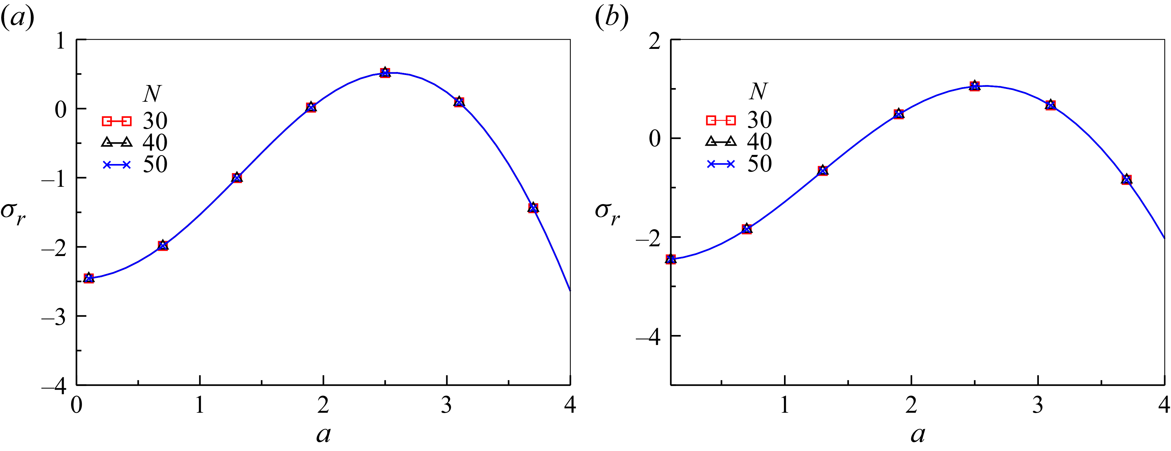
Influence of the order of Chebyshev polynomials (
 $N$
) on the growth rate of the disturbance.

Similarly, the eigenvalue problem corresponding to (2.71)–(2.74) for the nonlinear stability analysis can be written as
 \begin{equation} A_2X = \textit{RB}_2X. \end{equation}
The matrices
 $A_2$
and
 $B_2$
are given by
 \begin{equation} A_2= \begin{pmatrix} 2g_1(z)(4D^2-a^2I)+4g_1'(z)D & 0 & 0 \\[7pt] 0 & 2g_1(z)I & 0 \\[7pt] 0 & 0 & 2\eta (4D^2-\xi a^2I) \end{pmatrix}\!, \end{equation}
and
 \begin{equation} B_2= \begin{pmatrix} 0 & 0 & -b_{13} \\[7pt] 0 & 0 & a ^2\sin \phi \,I \\[7pt] -b_{31} & -\dfrac {\sin \phi }{a^2}I & 0 \end{pmatrix}\!, \end{equation}
where
 \begin{equation} b_{13}= \frac {Q\eta a^{2}}{2\varGamma }(z+1) +2ia_x\sin \phi \,D +a^{2}\cos \phi \,I, \end{equation}
and
 \begin{equation} b_{31}=\frac {Q\eta }{2\varGamma }(z+1) +\frac {2ia_x\sin \phi }{a^{2}}\,D +\cos \phi \,I. \end{equation}
The accuracy of the Chebyshev-tau technique can be determined through convergence analysis with respect to the number of collocation points
 $(N)$
. This is accomplished by comparing the growth-rate curves
 $(\sigma _r$
 $vs$
 $a)$
for varying numbers of collocation points for both longitudinal (figure 2
a) and transverse (figure 2
b) rolls at
 $Q = 1$
. The other fixed parameters are
 $\phi =30^\circ , \, \xi =1,\,\textit{Ra} = 100$
and
 $\varGamma = 0.5$
. The results show that the growth rate of the most unstable mode
 $\sigma _r$
initially rises with
 $a$
, attains a maximum at the most unstable wavelength and subsequently declines, becoming negative at approximately
 $a=3$
for longitudinal rolls (figure 2
a) and
 $a=2.6$
for transverse rolls (figure 2
b). This behaviour defines the cutoff wavelength, beyond which perturbations are stable. Furthermore, the growth-rate curves were obtained for different orders of the Chebyshev polynomial
 $(N)$
. The results show that increasing N leads to a converged solution. Based on this analysis, all computations in this study use
 $N=40$
for numerical accuracy.
The validation of numerical results based on the Chebyshev-tau-QZ method has been demonstrated in two ways. First, the comparison of the numerical solution of (2.21)–(2.23) based on the Chebyshev-tau-QZ method is validated by the Galerkin method for the stationary convection (
 $\sigma =0$
). More information on the Galerkin method is provided in the Appendix A. Table 1 presents a comparison of the critical Rayleigh number
 $(\textit{Ra}_{c})$
obtained using the Chebyshev-tau-QZ spectral method and the five-term (i.e.
 $k =5$
) Galerkin method, with the values of parameters
 $\xi =1$
,
 $\phi =0^\circ$
and
 $\varGamma = 0.5$
chosen. The results from the two approaches are in excellent agreement, thereby validating the numerical method’s reliability. To further validate the numerical solution of (2.21)–(2.23) based on the Chebyshev-tau-QZ method, a limiting case corresponding to the viscosity parameter
 $(\varGamma \to 0)$
and
 $(Q\to 0)$
, such that
 $Q/ \varGamma$
becomes unity with the other parameter values are
 $\phi = 0^\circ$
and
 $\xi = 1$
. Under these conditions, the present model reduces to the problem studied by Barletta & Nield (Reference Barletta and Nield2012) for longitudinal rolls. The computed value of the critical Rayleigh number is
 $\textit{Ra}_{c} = 61.8663$
for
 $a_{c} = 2.44826$
. Which shows the excellent alignment with those reported by Barletta & Nield (Reference Barletta and Nield2012).
Comparison of the critical Rayleigh numbers (
 $\textit{Ra}_{c}$
) obtained using the Chebyshev-tau-QZ spectral method and the Galerkin method for different values of
 $Q$
.

Table 1. Long description
The table presents a comparison of critical Rayleigh numbers (Rac) obtained using the Chebyshev-tau-QZ method and the Galerkin method for different values of Q. The table has three rows and three columns. The columns are labeled ‘Q’, ‘Chebyshev-tau-QZ (Rac)’, and ‘Galerkin (Rac)’. The row labels and values are as follows: Row 1: Q, 0.5; Chebyshev-tau-QZ (Rac), 51.8349; Galerkin (Rac), 51.8318. Row 2: Q, 1.0; Chebyshev-tau-QZ (Rac), 20.5550; Galerkin (Rac), 20.5519. Row 3: Q, 1.5; Chebyshev-tau-QZ (Rac), 9.6724; Galerkin (Rac), 9.6763.
3. Results and discussion
This study analyses the linear and nonlinear stability results presented for the onset of convection in an inclined porous medium described by Darcy–Forchheimer flow. The influences of anisotropic thermal diffusivity, an internal heat source and temperature-dependent viscosity are considered. The stability of fluid flow is determined by five major non-dimensional parameters: the Rayleigh number (
 $\textit{Ra}$
), inclination angle (
 $\phi$
), anisotropic thermal diffusivity parameter (
 $\xi$
), internal heat source (
 $Q$
) and viscosity parameter (
 $\varGamma$
). In this section, lines without symbols represent the results of
 $Q = 0.5$
, and lines with symbols indicate the results of
 $Q = 1$
.
Demonstration of linear instability (solid lines) and nonlinear stability (dashed lines), where
 $\textit{Ra}_{c}$
is plotted against
 $\xi$
for various values of
 $\phi$
with
 $\varGamma = 0.5$
for (a) longitudinal rolls and (b) transverse rolls.

Figures 3(a) and 3(b) present the linear (solid lines) and nonlinear (dashed lines) instability boundaries, where
 $\textit{Ra}_{c}$
is drawn against
 $\xi$
for different values of
 $\phi$
with
 $\varGamma = 0.5$
, such that figure 3(a) is for longitudinal rolls and figure 3(b) is for transverse rolls. From these figures, it is very clear that a rise in
 $\xi$
leads the system to be more stable. Note that
 $\xi$
represents the ratio of horizontal to vertical thermal diffusivity. Since a rise in
 $\xi$
increases horizontal thermal diffusivity, this results in a reduced rate of heat diffusion within the medium, decreasing its buoyancy force and thus stabilising the convection. More particularly, if the horizontal part of the thermal diffusivity is significantly greater than the vertical part (
 $\xi \gt 1$
), the medium exhibits greater stability and acts like an insulating substance. In contrast, if the vertical component of thermal diffusivity predominates over the horizontal components (
 $\xi \lt 1$
), convection is facilitated by decreasing
 $\textit{Ra}_{c}$
. This phenomenon has been observed in the literature Mourya & Kumar (Reference Mourya and Kumar2024). It has also been observed that higher inclination angles correlate with higher
 $\textit{Ra}_{c}$
, hence enhancing stability. It is important to note that
 $\textit{Ra}_{c}$
values decrease with increasing heat source strength, confirming the destabilising influence of the internal heat source across all values of
 $\phi$
in both linear and nonlinear stability cases, as seen in both graphs. Further, it is noted that the region of subcritical instability (i.e. the gap between linear and nonlinear stability) exists and increases with values of
 $\xi$
.
The comparison of figures 3(a) and 3(b) indicate that, when the inclination angle is absent (i.e. the porous layer is horizontal), the
 $\textit{Ra}_{c}$
values for longitudinal rolls and transverse rolls coincide for both
 $Q=0.5$
and
 $Q = 1$
. However, with an increasing value of
 $\phi$
, it shows that the value of
 $\textit{Ra} _{c}$
in transverse rolls is lower compared with longitudinal rolls. This shows that transverse rolls are more unstable compared with longitudinal rolls.
Demonstration of linear instability (solid lines) and nonlinear stability (dashed lines), where
 $\textit{Ra}_{c}$
is plotted against
 $\varGamma$
for different values of
 $\phi$
with
 $\xi = 1$
for (a) longitudinal rolls and (b) transverse rolls.

Figure 4. Long description
Two line graphs illustrate the relationship between Ra_c and Γ for different values of φ. Panel A: The line graph shows the relationship for longitudinal rolls. The x-axis represents Γ, ranging from 0 to 0.8, and the y-axis represents Ra_c, ranging from 0 to 120. The graph includes solid lines for linear instability and dashed lines for nonlinear stability. Different colors represent different values of φ: red for 0, blue for 30, and black for 45. An inset zooms in on the lower range of Γ from 0 to 0.8 and Ra_c from 0 to 12. Panel B: The line graph shows the relationship for transverse rolls. The x-axis represents Γ, ranging from 0 to 0.8, and the y-axis represents Ra_c, ranging from 0 to 100. Similar to Panel A, it includes solid lines for linear instability and dashed lines for nonlinear stability, with different colors representing different values of φ: red for 0, blue for 30, and black for 45. An inset zooms in on the lower range of Γ from 0 to 0.8 and Ra_c from 0 to 12.
The linear (solid lines) and nonlinear (dashed lines) stability theories are shown in figures 4(a) and 4(b), where
 $\textit{Ra}_c$
is plotted against
 $\varGamma$
for both
 $Q = 0.5$
(lines without symbols) and
 $ Q = 1$
(lines with symbols), respectively, such that figure 4(a) is for longitudinal rolls and figure 4(b) is for transverse rolls. The
 $\textit{Ra}_{c}$
values increase with
 $\varGamma$
, i.e. the parameter
 $\varGamma$
contributes to system stabilisation. This is because an increase in
 $\varGamma$
values makes the fluid thicker, which enhances intermolecular forces among the fluid particles, thereby reducing the effect of buoyancy forces and making it difficult for convection to begin, leading to the stabilisation of the flow. On the other hand, as the inclination angle increases, the
 $\textit{Ra}_{c}$
values also increase in both figures 4(a) and 4(b), indicating that inclination angles further aid in stabilising the system. From both graphs, it can also be observed that the presence of a stronger internal heat source (Q = 1) is more destabilising than that of a less internal heat source (Q = 0.5), as the internal heat source raises the system’s overall temperature.
In figure 4(a), it is noted that the values of
 $\textit{Ra}_{c}$
are lower in nonlinear theory as compared with linear theory for both
 $Q=0.5$
and
 $Q = 1$
. It can also be observed that the region of subcritical instability exists for both
 $ Q = 0.5$
and
 $Q = 1$
, suggesting that the linear theory may fail to simulate the physical phenomenon of convective motion appropriately.
Figure 4(b) shows the variation of
 $\textit{Ra}_{c}$
with
 $\varGamma$
for transverse rolls. The instability curves for linear and nonlinear theory follow the same pattern as in figure 4(a), but the values of
 $\textit{Ra}_{c}$
are smaller in transverse rolls. This shows that transverse rolls are less stable compared with longitudinal rolls.
Demonstration of linear instability (solid lines) and nonlinear stability (dashed lines), where
 $\textit{Ra}_{c}$
is plotted against
 $\phi$
for different values of
 $\xi$
with
 $\varGamma = 0.5$
for (a) longitudinal rolls and (b) transverse rolls.

Figures 5(a) and 5(b) show the stability curves for both linear (solid lines) and nonlinear (dashed lines) theories drawn
 $\textit{Ra}_c$
against
 $\phi$
for various values of
 $\xi$
with
 $\varGamma =0.5$
, such that figure 5(a) is for longitudinal rolls and figure 5(b) is for transverse rolls. It is observed that the
 $\textit{Ra}_{c}$
value enhances monotonically with rising values of inclination angle in both longitudinal and transverse rolls. Thus, convection is delayed as
 $\phi$
increases. The stabilising effect results from the diminished effect of buoyancy, the primary driving force in Rayleigh convection, when the medium is inclined. The physical reason for this is that
 $g\,\rm sin \phi$
and
 $ g\,\rm cos\phi$
act along the negative
 $x$
and
 $z$
axes, respectively. As the
 $\phi$
value increases, the gravitational component perpendicular to the layer diminishes, thereby lowering the effective unstable density stratification in the wall-normal direction. Consequently, the buoyancy force responsible for convection is suppressed. Analogous to figure 4, the internal heat source exerts a destabilising influence on both longitudinal and transverse rolls, since it enhances the buoyancy force, hence increasing system instability and precipitating early convection. From figure 5(a), it is seen that the region of subcritical instability expands with rising values of
 $\phi$
. In figure 5(b), it is noticed that the nonlinear stability graphs exhibit the same pattern as the linear ones. However, for differing values of
 $\xi$
, the
 $\textit{Ra}_c$
value increases throughout various ranges of
 $\phi$
and eventually begins to decrease as
 $\phi$
rises. It is also observed that for all values of
 $\xi$
, a region of subcritical instability occurs and enlarges with increasing values of
 $\phi$
as
 $\xi$
decreases.
Figures 6(a) and 6(b) depict the variations of
 $\textit{Ra}_{c}$
against
 $Q$
for different values of
 $\phi$
, such that figure 6(a) is for longitudinal rolls and figure 6(b) is for transverse rolls. It is noted that, as the values of
 $Q$
increase, the
 $\textit{Ra}_{c}$
values decrease in both linear and nonlinear analyses. This shows that increasing the internal heat source increases the heat transfer rate, thereby destabilising the system and leading to an earlier onset of convection. The physical reason is that an internal heat source raises the medium’s global temperature, resulting in a steeper temperature gradient that enhances buoyancy and destabilises the system. Furthermore, it can be seen that an increase in the inclination angles results in a higher
 $\textit{Ra}_{c}$
, suggesting enhanced stability. In figure 6(a), it is seen that the region of subcritical instability shrinks as
 $Q$
rises. For transverse rolls (figure 6
b), while the instability curves exhibit a similar tendency to that in figure 6(a), the
 $\textit{Ra}_{c}$
values are lower than those for longitudinal rolls. This indicates that the transverse rolls are more unstable than the longitudinal rolls.
Demonstration of linear instability (solid lines) and nonlinear stability (dashed lines), where
 $\textit{Ra}_{c}$
is plotted against
 $Q$
for different values of
 $\phi$
with
 $\xi = 1$
and
 $\varGamma = 0.5$
for (a) longitudinal rolls (b) transverse rolls.

Figure 6. Long description
Two line graphs are presented side by side. Panel A and Panel B each show the relationship between Ra_c and Q for different values of phi. The x-axis in both graphs represents Q, ranging from 0 to 1.5. The y-axis represents Ra_c, ranging from 0 to 400 in Panel A and from 0 to 300 in Panel B. Each graph includes three lines, colored red, blue, and black, corresponding to phi values of 0, 30, and 45, respectively. The solid lines indicate linear instability, while the dashed lines indicate nonlinear stability. Insets in both graphs provide a zoomed-in view of the data for Q values ranging from 0.3 to 1.5 and Ra_c values up to 20. The trends show that Ra_c decreases as Q increases for all values of phi, with the red line (phi = 0) consistently showing higher Ra_c values compared to the blue and black lines.
Streamlines when
 $ Q = 0.1$
. For (a)
 $\phi = 15^\circ$
, (b)
 $ \phi = 30^\circ$
and (c)
 $ \phi = 60^\circ$
with
 $\xi =1$
and
 $ \varGamma =0.5$
, plotted at the critical values
 $ \textit{Ra}_{c}$
and
 $a_{c}$
.

Streamlines when
 $ Q = 1$
. For (a)
 $\phi = 15^\circ$
, (b)
 $ \phi = 30^\circ$
and (c)
 $\phi = 60^\circ$
with
 $\xi =1$
and
 $ \varGamma =0.5$
, plotted at the critical values
 $ \textit{Ra}_{c}$
and
 $ a_{c}$
.

Streamlines when
 $ Q = 1.5$
. For (a)
 $\phi = 15^\circ$
, (b)
 $ \phi = 30^\circ$
and (c)
 $\phi = 60^\circ$
with
 $\xi =1$
and
 $\varGamma =0.5$
, plotted at the critical values
 $ \textit{Ra}_{c}$
and
 $ a_{c}$
.

4. Streamline plot
Figures 7–9 show the patterns of streamlines at various values of
 $\phi$
and
 $Q$
, which are plotted on the
 $(x,z)$
plane. The range of
 $z$
coordinates is taken from 0 to 1, whereas the range of
 $x$
coordinates is taken from 0 to
 $2\pi /a_{c}$
. The other fixed parameter values are
 $\varGamma = 0.5$
and
 $\xi = 1$
. Figure 7(a–c) is drawn at
 $Q = 0.1$
. Figure 8(a–c) is drawn at
 $Q = 1$
, and figure 9(a–c) is drawn at
 $Q = 1.5$
. From figure 7(a–c), it is notable that, for the smaller inclination angle (
 $\phi = 15^\circ$
), the flow exhibits a nearly symmetric single convection cell occupying the central region of the domain. The streamlines form closed elliptical contours, indicating that the vertical component of buoyancy remains dominant. As the angle of inclination rises to
 $\phi =30^\circ$
, the convective rolls exhibit a distinct tilt in the direction of the inclination. The flow’s symmetry about the central region diminishes. For a larger inclination of
 $(\phi =60^\circ )$
, the streamline pattern exhibits significant distortion and pronounced asymmetry. The counter-rotating rolls are markedly inclined, and the streamline attains its peak amplitude among the three scenarios. Increasing the inclination angle gradually disrupts the symmetry of the flow structure. The shift from a nearly symmetric central roll to a markedly displaced and skewed convection cell illustrates the substantial impact of inclination on stability attributes and nonlinear flow arrangement. The alteration in streamline topology is due to the fluctuation in the buoyancy forcing term, wherein the relative contributions of the vertical and horizontal components of gravity vary with
 $\phi$
. Furthermore, it can also be observed from figure 7–9 that, on increasing the values of
 $Q$
, the magnitude of the streamline increases, which shows convection occurs faster at higher
 $ Q$
.
5. Concluding remarks
In this study, the investigation focuses on analysing Darcy–Forchheimer convection in an inclined porous medium including the effect of anisotropic thermal diffusivity and the internal heat source through linear and nonlinear stability theories. The dynamic viscosity and density are assumed to have a linear temperature dependence. Linear instability analysis identifies the critical Rayleigh number by solving a generalised eigenvalue problem, while nonlinear stability theory is assessed using the energy method, which shows that
 $L^2$
theory fails to yield unconditional results. Therefore, to overcome this, an analysis using the higher-order norms was conducted, and it was found that the flow is conditionally stable for
 $Q \leqslant 2$
. The results show that increasing the thermal diffusivity parameter,
 $\xi$
, horizontally reduces the rate of heat diffusion within the fluid, decreases the buoyancy force and thus demonstrates a stabilising effect on porous media. The nonlinear stability boundaries are always lower than the linear boundaries in all cases, indicating that a subcritical instability region exists. Furthermore, it is shown that the critical Rayleigh number increases with increasing inclination angle and viscosity parameter, indicating that inclination and viscosity act as a stabilising mechanism by reducing the buoyancy force. On the other hand, the increasing heat source increases the heat transfer rate, thereby enhancing convective motion. Thus, the findings of this research have several practical applications across various geological and engineering fields, such as volcanology, glass manufacturing, thermal insulation and cooling systems, where the present analysis helps identify critical conditions and may assist in designing systems that optimise heat transfer. In such applications, the temperature-dependent viscosity of the fluid is a major factor influencing the direction of circulation and thus significantly contributes to optimising and stabilising convective heat transfer.
Acknowledgements
Pallawi Bharti acknowledges her gratitude to IIT (ISM) Dhanbad, India, for providing financial support. The authors thank the Associate Editor and referees for their constructive comments, which significantly improved the quality of the manuscript.
Declaration of interests
The authors report no conflict of interest.
Appendix A. Galerkin method
The Galerkin method is a weighted residual method (Finlayson & Scriven Reference Finlayson and Scriven1966), which approximates solutions to differential eigenvalue problems by expanding the dependent variables in terms of trial functions that satisfy the boundary conditions. Hence,
 $ W(z)$
and
 $\theta (z)$
are expanded as
 \begin{equation} W(z) = \sum _{k=1}^{n} A_{k} W_{k}(z),\, \theta (z) = \sum _{k=1}^{n} B_{k} \theta _{k}(z), \end{equation}
where
 $W_{k}(z) = \sin (k\pi z), \,\theta _{k}(z) = \cos ( {(2k-1)\pi z}/{2} )$
, and
 $A_{k}$
and
 $B_{k}$
are constants. Substituting (A1) into (2.21)–(2.22) we obtain residuals for the stationary convection. The Galerkin approach implies that each residual is orthogonal to its associated trial function. This gives a system of homogeneous linear equations in
 $A_{k}, B_{k}$
, which is obtained as
 \begin{equation} \begin{aligned} K_{ik}^{W}A_k+L_{ik}^{W}B_k=0,\\[3pt] M_{ik}^{\theta }A_k+N_{ik}^{\theta }B_k=0, \end{aligned} \end{equation}
where
 \begin{equation} K_{ik}^{W} =\big \langle D^{2}W_k,W_i\big \rangle -a^{2}\left \langle W_k,W_i\right \rangle +\left \langle H(z)DW_k,W_i\right \rangle \!, \end{equation}
 \begin{equation} L_{ik}^{W} = ia_xR\sin \phi \, \left \langle G(z)D\theta _k,W_i\right \rangle +\textit{Ra}^{2}\cos \phi \,\left \langle G(z)\theta _k,W_i\right \rangle \!, \end{equation}
 \begin{equation} M_{ik}^{\theta }= \big \langle D^{2}\theta _k,\theta _i\big \rangle -\xi a^{2} \left \langle \theta _k,\theta _i\right \rangle \!, \end{equation}
 \begin{equation} N_{ik}^{\theta }=\frac {\textit{RQ}}{\varGamma } \left \langle zW_k,\theta _i\right \rangle \!, \end{equation}
where
 $i,k=1,2,\ldots ,n$
, and
 $ \langle f,g\rangle = \int _{0}^1 f(z) g(z) {\rm d}z$
. The system (A3)–(A6) can be written in matrix form as follows:
 \begin{equation} \boldsymbol{M}\begin{bmatrix} {A_{k}}\\[3pt] B_{k} \end{bmatrix} =\boldsymbol{0}, \end{equation}
where
 \begin{equation} \boldsymbol{M} = \begin{bmatrix} K_{ik}^{W} & L_{ik}^{W} \\[7pt] M_{ik}^{\theta } & N_{ik}^{\theta } \end{bmatrix}. \end{equation}
In order to get a non-trivial solution, the determinant of the coefficient matrix must be zero. The obtained characteristic equation provides the admissible values of the Rayleigh number, and the minimum of such a value corresponds to the critical Rayleigh number.


 N

 Rac
 Q

 Rac
 ξ
 ϕ
 Γ=0.5

 Rac
 Γ
 ϕ
 ξ=1

 Rac
 ϕ
 ξ
 Γ=0.5

 Rac
 Q
 ϕ
 ξ=1
 Γ=0.5

 Q=0.1
 ϕ=15∘
 ϕ=30∘
 ϕ=60∘
 ξ=1
 Γ=0.5
 Rac
 ac

 Q=1
 ϕ=15∘
 ϕ=30∘
 ϕ=60∘
 ξ=1
 Γ=0.5
 Rac
 ac

 Q=1.5
 ϕ=15∘
 ϕ=30∘
 ϕ=60∘
 ξ=1
 Γ=0.5
 Rac
 ac


