Wake behind a three-dimensional dry transom stern. Part 1. Flow structure and large-scale air entrainment

Kelli Hendrickson; Gabriel D. Weymouth; Xiangming Yu; Dick K.-P. Yue

doi:10.1017/jfm.2019.505

Wake behind a three-dimensional dry transom stern. Part 1. Flow structure and large-scale air entrainment

Published online by Cambridge University Press: 26 July 2019

Xiangming Yu and

Kelli Hendrickson*: Affiliation:
Department of Mechanical Engineering, Massachusetts Institute of Technology, Cambridge, MA 02139, USA
Gabriel D. Weymouth: Affiliation:
Department of Mechanical Engineering, Massachusetts Institute of Technology, Cambridge, MA 02139, USA
Xiangming Yu: Affiliation:
Department of Mechanical Engineering, Massachusetts Institute of Technology, Cambridge, MA 02139, USA
Dick K.-P. Yue: Affiliation:
Department of Mechanical Engineering, Massachusetts Institute of Technology, Cambridge, MA 02139, USA
*: †Email address for correspondence: khendrk@mit.edu

Article contents

Abstract
Introduction
Method
Simulation of a canonical three-dimensional dry transom stern
Wake characteristics and flow features
Air entrainment
Summary
Footnotes
References

Rights & Permissions

Abstract

We present high-resolution implicit large eddy simulation (iLES) of the turbulent air-entraining flow in the wake of three-dimensional rectangular dry transom sterns with varying speeds and half-beam-to-draft ratios $B/D$. We employ two-phase (air/water), time-dependent simulations utilizing conservative volume-of-fluid (cVOF) and boundary data immersion (BDIM) methods to obtain the flow structure and large-scale air entrainment in the wake. We confirm that the convergent-corner-wave region that forms immediately aft of the stern wake is ballistic, thus predictable only by the speed and (rectangular) geometry of the ship. We show that the flow structure in the air–water mixed region contains a shear layer with a streamwise jet and secondary vortex structures due to the presence of the quasi-steady, three-dimensional breaking waves. We apply a Lagrangian cavity identification technique to quantify the air entrainment in the wake and show that the strongest entrainment is where wave breaking occurs. We identify an inverse dependence of the maximum average void fraction and total volume entrained with $B/D$. We determine that the average surface entrainment rate initially peaks at a location that scales with draft Froude number and that the normalized average air cavity density spectrum has a consistent value providing there is active air entrainment. A small parametric study of the rectangular geometry and stern speed establishes and confirms the scaling of the interface characteristics with draft Froude number and geometry. In Part 2 (Hendrikson & Yue, J. Fluid Mech., vol. 875, 2019, pp. 884–913) we examine the incompressible highly variable density turbulence characteristics and turbulence closure modelling.

JFM classification

Wakes/Jets: Wakes Waves/Free-surface Flows: Wave breaking Multiphase and Particle-laden Flows: Multiphase flow

Information

Type: JFM Papers
Information: Journal of Fluid Mechanics , Volume 875 , 25 September 2019, pp. 854 - 883
DOI: https://doi.org/10.1017/jfm.2019.505 [Opens in a new window]
Copyright: © 2019 Cambridge University Press

1 Introduction

Our interest is the complex, three-dimensional wake immediately behind the dry transom stern of a surface ship. This region contains violent breaking of the free surface, highly mixed air–water turbulent flow, large-scale air entrainment and air cavity breakup. In addition to gaining fundamental scientific understanding, quantification and prediction of these features are of critical importance to the design and operation of surface ships. The objective of the present work is to perform implicit large eddy simulation (iLES) to elucidate and quantify the near wake of a dry transom, to complement and support the laboratory and field measurements and to inform bubble source and turbulence closure models used in large-scale (whole-ship) predictions (Baldy Reference Baldy1993; Jingsen et al. Reference Jingsen, Oberai, Hyman, Drew and Lahey2011; Ma, Shi & Kirby Reference Ma, Shi and Kirby2011). Presented in two parts, Part 1 focuses on the wake surface, the structure of the underlying wake flow, Lagrangian characteristics of the large-scale air entrainment and surface entrainment rate and the scaling of these with Froude number and stern geometry. The objective of this part is to provide a physical understanding of the detailed flow features in the mixed region and the characteristics of the large-scale air entrainment. Part 2 (Hendrickson & Yue Reference Hendrickson and Yue2019) focuses on understanding and modelling of the highly mixed, air–water turbulent near-surface region of the wake by combining the surface fluctuations, spray and entrainment into a single mixed-phase region through an Eulerian framework. The objective of this part is to provide a statistical understanding of the mixed-phase region within the context of incompressible highly variable density turbulence and address the necessary turbulent mass flux closure modelling.

While there are many studies of small-scale air entrainment such as for a surface impinging jet (Cummings & Chanson Reference Cummings and Chanson1997; Ohl, Oguz & Prosperetti Reference Ohl, Oguz and Prosperetti2000; Zhu, Oguz & Prosperetti Reference Zhu, Oguz and Prosperetti2000; Chanson & Manasseh Reference Chanson and Manasseh2003; Chanson, Aoki & Hoque Reference Chanson, Aoki and Hoque2004; Hoque & Aoki Reference Hoque and Aoki2008), the ship-wake problem presents special experimental and computational challenges. In addition to the complexities of the air–water interface and entraining turbulent flows, the (prototype) problem involves high void fractions (20 %–30 %) (Terrill & Fu Reference Terrill and Fu2008) and flow length scales spanning from the ship length, beam and draft $O(10^{1-2})~\text{m}$ down to micron-sized bubbles. Indeed, until recently, relatively little is understood or predictable about this flow.

Recent full-scale experiments of a transom stern vessel (Fu et al. Reference Fu, Fullerton, Terrill and Lada2006; Terrill & Fu Reference Terrill and Fu2008; Terrill & Taylor Reference Terrill and Taylor2015) and laboratory-scale experiments of a transom hull form (Drazen et al. Reference Drazen, Fullerton, Fu, Beale, O’Shea, Brucker, Dommermuth, Wyatt, Bhushan and Carrica2010) and breaking waves (Lamarre & Melville Reference Lamarre and Melville1991) provided significant insight into wake interface characteristics and statistics as well as initial information regarding the wake air entrainment. Based on images from experiments (Fu et al. Reference Fu, Fullerton, Drazen, Minnick, Walker, Ratcliffe, Russell and Capitain2010a ), the three-dimensional flow behind the transom stern is visually similar to the supercritical flow behind chute piers in spillways due to the presence of the characteristic rooster tail (Pagliara, Kurdistani & Roshni Reference Pagliara, Kurdistani and Roshni2011). Laboratory-scale experiments reported void fractions within 10 %–15 % and field-scale experiments at 20 %–30 %. Experiments at both scales reported the location of the bulk of the entrained air to be immediately aft of the stern in the rooster-tail region and confined within the depth of the wetted transom. Due to the complexity of full-scale at-sea measurements and measurements with high void fractions, there are currently no published data on the detailed flow structure or air entrainment in the mixed region of the wake of a ship at either scale.

State-of-the-art multiphase viscous flow simulations have advanced numerical capabilities for modelling the complex gas–liquid flows of hydraulic jumps, breaking waves, large-scale ships and planing hulls (Adams et al. Reference Adams, George, Stephens, Brucker, O’Shea and Dommermuth2010; Drazen et al. Reference Drazen, Fullerton, Fu, Beale, O’Shea, Brucker, Dommermuth, Wyatt, Bhushan and Carrica2010; Fu et al. Reference Fu, Ratcliffe, O’Shea, Brucker, Graham, Wyatt and Dommermuth2010b ; Fullerton et al. Reference Fullerton, Fu, Brewton, Brucker, O’Shea and Dommermuth2010; Deike, Melville & Popinet Reference Deike, Melville and Popinet2016; Mortazavi et al. Reference Mortazavi, Le Chenadec, Moin and Mani2016). Relevant to our effort is the simulation of the transom stern experiments at full and laboratory scale using both iLES and unsteady Reynolds-averaged Navier–Stokes (uRANS) flow solvers to compare to measured interface characteristics and statistics (Wyatt et al. Reference Wyatt, Fu, Taylor, Terrill, Xing, Bhushan, O’Shea and Dommermuth2008; Drazen et al. Reference Drazen, Fullerton, Fu, Beale, O’Shea, Brucker, Dommermuth, Wyatt, Bhushan and Carrica2010). In this work, the authors simulated both a wet and dry transom configuration and quantified the spectrum of the interface fluctuations. However, the work did not provide information on the flow structure or detailed void fraction information.

The only available information that may provide insight regarding the flow field in the mixed region is that of two-dimensional transom experiments (modelled as flow beneath a backward facing step Maki, Troesch & Beck Reference Maki, Troesch and Beck2008; Rodriguez-Rodriguez et al. Reference Rodriguez-Rodriguez, Marugan-Cruz, Aliseda and Lasheras2011) and two-dimensional supercritical hydraulic jumps (Hoyt & Sellin Reference Hoyt and Sellin1989; Chanson Reference Chanson1995; Mossa & Tolve Reference Mossa and Tolve1998; Chanson & Brattberg Reference Chanson and Brattberg2000; Chanson Reference Chanson2009; Chachereau & Chanson Reference Chachereau and Chanson2011; Lin et al. Reference Lin, Hsieh, Lin, Chang and Raikar2012; Mortazavi et al. Reference Mortazavi, Le Chenadec, Moin and Mani2016). Collectively, they report that the velocity field contains a mixing shear layer with coherent structures and a peak in the average void fraction in regions of large turbulent shear. Recent non-intrusive measurements of the velocity field in the mixed region (Lin et al. Reference Lin, Hsieh, Lin, Chang and Raikar2012) find that the presence of the large recirculation region in supercritical hydraulic jumps significantly alters the turbulent statistics. Direct numerical simulations (DNS) (Mortazavi et al. Reference Mortazavi, Le Chenadec, Moin and Mani2016) identify the average interface near the turbulent toe of the jump as a near-stagnant condition below which exists a recirculation region and above which is a jet-like profile. However, the similarity between these two-dimensional flows (both hydraulic jumps and transom sterns) and a three-dimensional wake behind a finite beam transom stern are yet to be understood.

The length scales of interest for this work (laboratory or prototype) are typically many orders of magnitude greater than the Hinze scale $a_{H}$ , above which cavity breakup is primarily due to shear and turbulent fluctuations, and below which surface tension and other small-scale effects become important in the bubble dynamics (Hinze Reference Hinze1955). For breaking waves, Deane & Stokes (Reference Deane and Stokes2002) report $a_{H}\sim O(1)~\text{mm}$ , while features in the stern wake could involve length scales $O(10)~\text{m}$ or more. Numerically resolving this range would require ${>}O(10^{12})$ grid points, which is computationally prohibitive. Thus, in our iLES, we focus on features greater than $O(a_{H})$ and ignore surface tension. The limitation of our results is the grid size $\unicode[STIX]{x1D6E5}\gg a_{H}$ and not neglection of sub-Hinze-scale surface tension effects. Strictly speaking, we resolve the air entrainment and cavity formation and breakup associated with the large-scale flow, but not the details of the air cavities/bubbles below $O(\unicode[STIX]{x1D6E5})$ .

We perform incompressible, two-phase (air–water) iLES on a three-dimensional Cartesian grid using a conservative volume-of-fluid (cVOF) method (Weymouth & Yue Reference Weymouth and Yue2010). The cVOF method conserves mass to machine precision, which is a critical component for quantitative prediction of air entrainment. The efficacious boundary data immersion (BDIM) method provides the body representation in the Cartesian grid. Motivated by work such as Drazen et al. (Reference Drazen, Fullerton, Fu, Beale, O’Shea, Brucker, Dommermuth, Wyatt, Bhushan and Carrica2010), we consider the problem of a canonical transom stern of rectangular cross-section (beam $2B$ , draft $D$ ) in deep water idealized as a partially submerged rectangular prism to remove upstream kinematic and geometric influences. To further simplify the problem, we assume uniform and constant-in-time inflow velocity $U$ outside the stern cross-section on the inflow plane. Thus, the parameters that characterize the problem are the half-beam-to-draft ratio $B/D$ and draft Froude number $Fr=U/\sqrt{gD}$ . We perform iLES for different $B/D$ ratios and dry transom values of $Fr$ .

Our simulations capture the characteristic features of the wake: the converging corner waves originating from the transom; the colliding of these waves aft of the near stern (an event that is geometry dependent) to form the ‘rooster tail’ and the development of a significant three-dimensional, mixed region near the surface; and subsequent formation of the V-shaped diverging wave wake as the rooster tail widens downstream. We elucidate the mean interface characteristics and define their scaling with ship-scale parameters $B/D$ and $Fr$ . We explore the mean flow field of the complex turbulent mixed-phase region and identify the presence of a jet and secondary vortex structure below the average interface. We show that the mixed region flow contains a shear region similar to that of two-dimensional hydraulic jumps and two-dimensional stern flows but there is no appreciable evidence that a recirculating region typical of those flows exists immediately aft of the three-dimensional geometry. The breaking waves further downstream in the diverging wave wake, reintroduce a three-dimensional flow structure that might resemble a roller bore with strong cross-stream advection on an oblique plane that directly influences the turbulent statistics and air entrainment in this region.

To identify the entrained air cavities, we develop an algorithm based on the connected component algorithm (CCA) (Samet & Tamminen Reference Samet and Tamminen1988) from computer graphics that enables quantification of the air entrainment and cavity size characteristics. We obtain the spatial distribution of the surface entrainment rate, which initially peaks in the converging-corner-wave region and has a second peak at the end of the rooster-tail region with the development of the V-shaped diverging-wave region. We observe void fractions of 13 % in the diverging-wave region, consistent with laboratory-scale experiments. When we consider the density spectra of cavity sizes $N(r)$ in different regions of the wake, we obtain a power-law spectrum $N(r)\sim r^{\unicode[STIX]{x1D6FD}}$ with slope $r^{\unicode[STIX]{x1D6FD}}$ that is weakly dependent on $B/D$ with $\unicode[STIX]{x1D6FD}>-4$ when there is active wave breaking.

The outline of this paper is as follows. Section 2 details the numerical procedure used to obtain the iLES datasets and outlines the Lagrangian cavity identification algorithm used to determine the entrained air cavity volumes. Section 3 defines the canonical ship-wake problem used in this study. Section 4 presents the analysis of the wake interface characteristics and the detailed description of the flow structure in the mixed region, including the average velocity and vorticity fields. Section 5 details the air entrainment results. Section 6 discusses the overall impact of the findings of this paper in the context of large-scale, three-dimensional ship wakes. The appendices contain verification information as well as the parameter study.

2 Method

2.1 Numerical procedure

We employ iLES of the two (assumed) incompressible fluids, air and water, using cVOF and BDIM on a Cartesian grid. The three-dimensional velocity field $\boldsymbol{u}(\boldsymbol{x})$ in a domain $\boldsymbol{x}$ obeys the continuity equation $\unicode[STIX]{x1D735}\boldsymbol{\cdot }\boldsymbol{u}=0$ and the momentum equation in the absence of surface tension,

(2.1)

$$\begin{eqnarray}\frac{\unicode[STIX]{x2202}\boldsymbol{u}}{\unicode[STIX]{x2202}t}+\unicode[STIX]{x1D735}\boldsymbol{\cdot }(\boldsymbol{u}\boldsymbol{u})=-\frac{1}{\unicode[STIX]{x1D70C}}\unicode[STIX]{x1D735}p+\frac{\boldsymbol{g}}{Fr^{2}},\end{eqnarray}$$

where $p$ is the total pressure field and $\boldsymbol{g}/Fr^{2}$ the gravitational vector scaled by Froude number $Fr$ . The volume fraction $f$ provides the density $\unicode[STIX]{x1D70C}$ using the two fluid densities $\unicode[STIX]{x1D70C}_{water}$ and $\unicode[STIX]{x1D70C}_{air}$ as

(2.2)

$$\begin{eqnarray}\unicode[STIX]{x1D70C}(\boldsymbol{x})=f(\boldsymbol{x})\unicode[STIX]{x1D70C}_{water}+[1-f(\boldsymbol{x})]\unicode[STIX]{x1D70C}_{air}.\end{eqnarray}$$

We capture the two-fluid interface using a fully conservative three-dimensional volume-of-fluid method, cVOF (Weymouth & Yue Reference Weymouth and Yue2010). As in standard VOF methods, $f$ derives from integrating the so-called fluid ‘colour function’, $c(\boldsymbol{x})$ defined as 1 or 0 in the water or air, respectively. The volume fraction $f$ within each computational volume $\unicode[STIX]{x1D6FA}$ represents the fraction of $c$ within each cell. A simple explicit operator-split update equation ensures conservative transport of the interface via $n$ sweeps over

(2.3)

$$\begin{eqnarray}\unicode[STIX]{x0394}f=\frac{\unicode[STIX]{x0394}t}{\unicode[STIX]{x0394}\unicode[STIX]{x1D6FA}}\mathop{\sum }_{d=1}^{n}\left(\unicode[STIX]{x1D6E5}_{d}F_{d}+c_{c}\frac{\unicode[STIX]{x2202}u_{d}}{\unicode[STIX]{x2202}x_{d}}\unicode[STIX]{x0394}\unicode[STIX]{x1D6FA}\right),\end{eqnarray}$$

where $n$ is the number of spatial dimensions, $u_{d}$ the velocity components, $\unicode[STIX]{x1D6E5}_{d}F_{d}$ the net fluxes of liquid fluid through the $d$ -face of the volume and $c_{c}$ is the cell centre value of the colour function given for linear interfaces by

(2.4)

$$\begin{eqnarray}c_{c}=\left\{\begin{array}{@{}ll@{}}1 & \text{if }f>1/2,\\ 0 & \text{else}.\end{array}\right.\end{eqnarray}$$

As shown in Weymouth & Yue (Reference Weymouth and Yue2010) the updates of (2.3) along with the Courant restriction on the time step $\unicode[STIX]{x0394}t$ of the form

(2.5)

$$\begin{eqnarray}\unicode[STIX]{x0394}t\mathop{\sum }_{d=1}^{n}\left|\frac{u_{d}}{\unicode[STIX]{x0394}x_{d}}\right|<\frac{1}{2}\end{eqnarray}$$

guarantee that the transport method is fully conservative for general flows.

We immerse the ship geometry in the Cartesian background grid with BDIM (Weymouth & Yue Reference Weymouth and Yue2011), which includes the effect of the solid body on the fluid by convolving the governing equations and interfacial conditions of any solid/fluid system with smooth, finite-width integration kernels. This results in a single governing equation for the complete domain. BDIM’s analytic formulation ensures proper treatment of general boundary conditions (Weymouth & Yue Reference Weymouth and Yue2011; Weymouth & Triantafyllou Reference Weymouth and Triantafyllou2013). This work focuses on simulation of stationary bodies immersed in a high Reynolds number flow with free-slip tangential velocity boundary conditions. As such our governing equations are velocity matching for the normal component of velocity $u_{n}$ on the interface

(2.6)

$$\begin{eqnarray}u_{n}(\boldsymbol{x}_{b})-{\mathcal{U}}(\boldsymbol{x}_{b})=0,\end{eqnarray}$$

where ${\mathcal{U}}$ is the interface flux, which is zero for solid boundaries. A homogeneous Neumann condition for the tangential velocity components ( $u_{\unicode[STIX]{x1D70E}}$ , $u_{\unicode[STIX]{x1D70F}}$ ) normal to the interface enforces a free-slip boundary condition on the body

(2.7a,b )

$$\begin{eqnarray}\frac{\unicode[STIX]{x2202}u_{\unicode[STIX]{x1D70E}}}{\unicode[STIX]{x2202}n}=0\quad \text{and}\quad \frac{\unicode[STIX]{x2202}u_{\unicode[STIX]{x1D70F}}}{\unicode[STIX]{x2202}n}=0.\end{eqnarray}$$

Combining (2.1), (2.6) and (2.7) using the BDIM formulation gives the global meta equation

(2.8)

$$\begin{eqnarray}\boldsymbol{u}+\boldsymbol{{\mathcal{L}}}(\boldsymbol{u})=\unicode[STIX]{x1D6FF}_{e}^{B}\boldsymbol{U}+[1-\unicode[STIX]{x1D6FF}_{e}^{B}]\left(\boldsymbol{u}(t_{0})+\int _{t_{0}}^{t_{0}+\unicode[STIX]{x0394}t}\left[\boldsymbol{r}-\frac{1}{\unicode[STIX]{x1D70C}}\unicode[STIX]{x1D735}p\right]\,\text{d}t\right).\end{eqnarray}$$

Here, $\boldsymbol{r}$ represents the convection and gravity terms and $\unicode[STIX]{x1D6FF}_{e}^{B}$ is the zeroth moment of the integration kernel over the body (approximated by a smoothed Heaviside function based on the distance to the body geometry). The left-hand side operator ${\mathcal{L}}$ is

(2.9)

$$\begin{eqnarray}\boldsymbol{{\mathcal{L}}}(\boldsymbol{u})\equiv \unicode[STIX]{x1D6FF}_{e}^{S}\frac{\unicode[STIX]{x2202}\boldsymbol{u}_{\unicode[STIX]{x1D70F}}}{\unicode[STIX]{x2202}n}\hat{\unicode[STIX]{x1D70F}}+\unicode[STIX]{x1D6FF}_{e}^{S}\frac{\unicode[STIX]{x2202}\boldsymbol{u}_{\unicode[STIX]{x1D70E}}}{\unicode[STIX]{x2202}n}\hat{\unicode[STIX]{x1D70E}},\end{eqnarray}$$

where $\unicode[STIX]{x1D6FF}_{e}^{S}$ is the zeroth moment of the integration kernel centred at the nearest point on the interface.

We discretize the governing equations using a staggered-grid finite volume method. The implicit modelling of iLES derives from a flux-limited QUICK (quadratic upstream interpolation for convective kinematics) treatment of the convective terms. An explicit second-order predictor–corrector method estimates the time integral in (2.8). Hereafter, we normalize all fluid constitutive properties to those of water: $\unicode[STIX]{x1D70C}=\unicode[STIX]{x1D70C}^{\ast }/\unicode[STIX]{x1D70C}_{water}$ and $\unicode[STIX]{x1D707}=\unicode[STIX]{x1D707}^{\ast }/\unicode[STIX]{x1D707}_{water}$ , where $\text{}^{\ast }$ denotes respectively the dimensional density and viscosity of the fluid at a given point. Finally, we determine the pressure via the projection method using the continuity equation. A multi-grid solver using conjugate-gradient smoothing inverts the pressure Poisson matrix. Verification of the method appears in appendix B as well as Weymouth & Yue (Reference Weymouth and Yue2010, Reference Weymouth and Yue2011), Weymouth et al. (Reference Weymouth, Hendrickson, Banerjee and Yue2010) and Hendrickson et al. (Reference Hendrickson, Weymouth, Banerjee and Yue2013).

2.2 Air cavity identification

The air–water interface of high-energy flows possesses non-trivial topological complexity. The forthcoming analysis requires us to identify air entrainment (defined as a cavity of air not connected to the bulk air volume), the bulk water volume (defined as the water volume with spray droplets removed and air cavities filled) and the mixed-phase volume (defined as the original $f$ field). To identify spray droplets and air cavities, we develop a method of identifying contiguously connected regions of the three-dimensional, time-varying air volume fraction field $f_{a}\equiv 1-f(\boldsymbol{x},t)$ . The method is a modified version of a two-pass standard CCA algorithm (Samet & Tamminen Reference Samet and Tamminen1988). The algorithm enables the calculation of the individual air cavities $v_{e}^{i}=\int \hat{f}_{ai}(\boldsymbol{x})\,\text{d}\boldsymbol{x}$ and effective spherical radius $r_{eff}^{i}=[(3/4\unicode[STIX]{x03C0})v_{e}^{i}]^{1/3}$ . The unique identifiers that result in the CCA algorithm identify the air cavities in $f$ and spray droplets in $f_{a}$ that are either filled or removed to calculate the water bulk region in § 4.2. Appendix A further discusses the details of this Lagrangian analysis technique.

3 Simulation of a canonical three-dimensional dry transom stern

The canonical problem we consider is the flow behind a rectangular transom stern of half-beam $B$ and still water draft $D$ . We scale by the draft $D$ and the uniform steady inflow velocity $U$ . The draft Froude number $Fr=U/\sqrt{gD}$ characterizes this problem. The cases considered are at sufficiently high $Fr$ to correspond to dry transom conditions. Recent experiments of Drazen et al. (Reference Drazen, Fullerton, Fu, Beale, O’Shea, Brucker, Dommermuth, Wyatt, Bhushan and Carrica2010) using a Model 5674 geometry with draft of $D=0.305~\text{m}$ showed that transition to dry transom conditions occurred between 7 and 8 kts or $Fr=2.38$ at laboratory scale. Performing many iLES over a range of $Fr2.38\leqslant Fr\leqslant 3$ and half-beam-to-draft $B/D$ ratios $1\leqslant B/D\leqslant 2.1$ , we find that the results are qualitatively similar, and can be described with a set of representative cases A, B and C (details in table 1).

The boundary conditions for the Cartesian grid iLES (figure 1) are as follows: (i) uniform inflow velocity $U$ on the inlet plane except its intersection with the rectangular body geometry where the body boundary conditions are enforced as described in § 2.1; (ii) zero-gradient extrapolations on the lateral boundaries; (iii) symmetry planes for the top and bottom boundaries; and (iv) mass conserving exit condition far downstream. We subdivide the computational domain into a high-resolution inner interrogation domain of constant grid volume $\unicode[STIX]{x1D6FF}\unicode[STIX]{x1D6FA}=\unicode[STIX]{x1D6E5}^{3}$ that encompasses the near region behind the stern. Our interest is the large-scale features of the air-entraining turbulent wake extending horizontally $O(10D)$ behind the stern. Thus, we size the interrogation domain to be $L_{x}\times L_{y}\times L_{z}=13D\times 10D\times 3D$ where $x,y,z$ are respectively the longitudinal, transverse and vertical dimensions. The interrogation grid resolution is $\unicode[STIX]{x1D6E5}=D/64$ . This is sufficient to resolve features an order of magnitude smaller than $D$ , but the numerical Hinze scale $a_{N}=\unicode[STIX]{x1D6E5}\sim 1~\text{cm}$ is still substantially greater than the physical Hinze scale $a_{H}$ for realistic laboratory-scale (and certainly full-scale) stern experiments (Fu et al. Reference Fu, Fullerton, Terrill and Lada2006; Terrill & Fu Reference Terrill and Fu2008; Drazen et al. Reference Drazen, Fullerton, Fu, Beale, O’Shea, Brucker, Dommermuth, Wyatt, Bhushan and Carrica2010). A buffer domain that employs algebraic grid stretching surrounds the interrogation domain, extending the outer boundaries and increasing the numerical damping in the transverse and far-stream regions. The entire Cartesian grid (interrogation and buffer domain) is $N_{x}\times N_{y}\times N_{z}=1024\times 896\times 256=2.35\times 10^{8}$ spatial grid cells.

We initiate the simulation by linearly increasing the inflow velocity over a period of $t=TU/D=10$ . Once at a quasi-steady state, we sample the interrogation domain to obtain time-averaged statistics over $80\leqslant t\leqslant 120$ with a sampling rate at $\text{d}t=0.01$ . All averages reported herein are temporal averages over this period of time with this sample rate. Table 1 reports the median $\unicode[STIX]{x1D708}_{e}^{m}$ and third-quartile $\unicode[STIX]{x1D708}_{e}^{3rd}$ value of the iLES effective viscosity (defined in appendix B).

Figure 1.

Schematic of the canonical stern geometry. Blue area: the high-resolution interrogation domain $L_{x}\times L_{y}\times L_{z}=13D\times 10D\times 3D$ .

Table 1.

Parameters for representative cases A, B and C measured within the interrogation domain. $\unicode[STIX]{x1D708}_{e}^{m}$ and $\unicode[STIX]{x1D708}_{e}^{3rd}$ are the median and third-quartile values of the iLES effective viscosity (defined in appendix B). The time step $\unicode[STIX]{x0394}t=1.875\times 10^{-3}$ .

We utilize three different analysis techniques throughout Part 1 and Part 2. In § 4.2, we use the modified CCA of § 2.2 and appendix A to isolate the connected isosurface that represents the unbroken air–water interface and water bulk region by removing both air bubbles and spray droplets. We use a temporal average of the resulting bulk fraction $\overline{f_{b}}$ to identify the surface region, where $0<\overline{f_{b}}<1$ incorporates only surface fluctuations and $\overline{f_{b}}=0.5$ represents the mean interface. In § 4.3, we use a purely Eulerian framework with unconditioned time averages where $0<\overline{\unicode[STIX]{x1D70C}}<1$ represents the mixed-phase region (or mixed region) which incorporates surface fluctuations, entrainment and spray. Part 2 uses this framework exclusively and uses the turbulent mass flux $\overline{\unicode[STIX]{x1D70C}u_{i}^{\prime }}$ to represent all of these physical processes as a single vector quantity. In § 5, we adopt a Lagrangian framework to focus solely on the air entrainment. Using the modified CCA to identify air bubbles, we calculate the bubble statistics and define the entrainment envelope from a temporal average of $v_{e}$ on the Cartesian grid. Figure 2 shows the conceptual difference between the entrainment envelope, mixed region and surface region using a transverse cut in the far wake (looking upstream). Note that the lines for $\overline{f}=\overline{f_{b}}=0.5$ coincide, as expected.

Figure 2.

Comparison of entrainment envelope, surface region and the mixed region for a transverse cut at $x=11.5$ . Green lines $\overline{f}$ and red lines $\overline{f_{b}}=(0.01,0.5,0.99)$ from top to bottom within each figure, respectively. Blue region is $\overline{v_{e}}\geqslant 0.01$ . Data are case B.

4 Wake characteristics and flow features

4.1 General wake features

Figures 3, 4 and 5 shows the isosurface of the instantaneous volume fraction $f=0.5$ for respectively cases A, B and C. All cases have three distinct characteristic regions in the surface of the wake, which we refer to hereafter as the converging-corner-wave (CCW), the rooster-tail (RT) and the diverging-wave (DW) regions. The first region contains a large depression behind the dry stern with ridges that rise from the lower corner. These ridges, or CCW, angle in towards the centreline of the ship. After the CCW region is the RT, the length of which decreases with $B/D$ . The surface of the RT is rough with many small ligaments and spray. The RT region widens to form the beginning of the DW train behind the stern. Here, the centre of the wake surface becomes smoother and the edges contain very fine structures and quasi-steady breakers. Scars on the interface (indicated by the dark features angling away from the centreline) indicate regions of wave overturning and air entrainment similar to those observed by (for example) Dong, Katz & Huang (Reference Dong, Katz and Huang1997) and Olivieri et al. (Reference Olivieri, Pistani, Wilson, Campana and Stern2007) for overturning bow waves.

While each wake contains these distinct characteristic regions, there are overall differences in the wake between cases A/B and case C. For cases A and B, the CCW collide on the ship centreline before overturning and entraining a fully formed air cavity. The physics at this collision point represent two impacting jets and serve as a source of significant spray. For case C, the CCW have ample time to break and entrain air before the formation of the RT. Because of this, the RT in case C is smoother with less spray and ligaments than cases A and B.

Figure 3.

Instantaneous isosurface of volume fraction $f=0.5$ for case A within the interrogation domain. Flow is from left to right ( $+x$ ). (a) Viewed from above; (b) viewed from the side. Surface is rendered partially transparent. Dark regions indicate multi-valued surface, spray or entrainment. See also the corresponding supplementary movies 1 and 2 available at https://doi.org/10.1017/jfm.2019.505.

Figure 4.

As in figure 3 for case B. See also corresponding supplementary movies 3 and 4.

Figure 5.

As in figure 3 for case C. See also corresponding supplementary movies 5 and 6.

4.2 Wake characteristics and scaling

We obtain a cleaner depiction of the instantaneous surface by utilizing the cavity identification algorithm of § 2.2 to identify the air cavities and spray droplets and either filling them (if air) or removing them (if water). The resulting instantaneous bulk volume fraction $f_{b}$ is the result. Figure 6 shows the time-averaged isosurface of $f_{b}$ corresponding to $\overline{f_{b}}=0.5$ for case A (case B is similar). The location where the CCW collide on the centreline $x_{c}$ appears different when viewed from above (figure 6 a) and below (figure 6 b) due to the multi-valued nature of the interface. The RT is present for $x>x_{c}$ . At a point further downstream, the waves radiate away from the centreline and form a divergent wave pattern.

Figure 6.

Average interface $\overline{f_{b}}=0.5$ case A. (a) Viewed from above and (b) below. Contours represent elevation $z$ (light to dark, negative to positive). - - - $x_{c}$ . Note that the ‘ripples’ on the interface near the inlet are an artefact of the visualization of the isosurface and not present in the simulation.

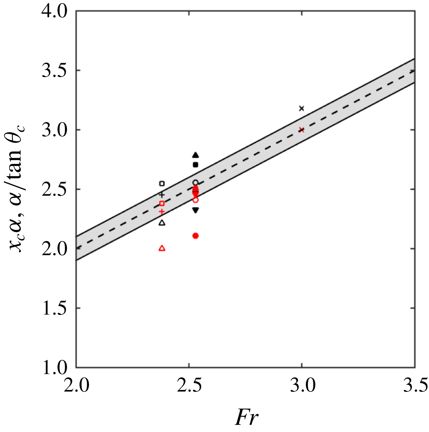
The experiments of Martínez-Legazpi et al. (Reference Martínez-Legazpi, Rodríguez-Rodríguez, Marugán-Cruz and Lasheras2013) established that the trajectory of the wavefront emanating from the corner of a partially submerged vertical plate is ballistic by considering the impact point of the corner wave on the surface downstream of the plate. A similar potential energy argument for the stern geometry provides the scaling of $x_{c}$ . Consider the flow leaving the bottom corner of the stern at $x=0$ with speed $(U,v_{0},w_{0})$ . Assuming the velocity in the $y{-}z$ plane is gravity driven, the $y{-}z$ plane velocity $(v_{0},w_{0})=\sqrt{2gD}\;(\cos \unicode[STIX]{x1D719}_{c},\sin \unicode[STIX]{x1D719}_{c})$ where $\unicode[STIX]{x1D719}_{c}$ is the angle of the projectile motion in the $y{-}z$ plane (see figure 7 a). The time for a particle to travel the distance $B$ to the centreline, assuming $v_{0}$ and $U$ constant, provides the location where the corner waves meet and the angle of the waves in the $x{-}y$ plane $\unicode[STIX]{x1D703}_{c}$ as,

(4.1a,b )

$$\begin{eqnarray}x_{c}=FrB\unicode[STIX]{x1D6FC}^{-1}\quad \text{and}\quad \tan \unicode[STIX]{x1D703}_{c}=\unicode[STIX]{x1D6FC}Fr^{-1},\end{eqnarray}$$

where $\unicode[STIX]{x1D6FC}=\sqrt{2}\cos \unicode[STIX]{x1D719}_{c}$ . Thus for a dry rectangular transom stern, $Fr$ , $B$ and $\unicode[STIX]{x1D719}_{c}$ completely determine the location of the collision of the CCW and the beginning of the RT. This ballistic behaviour and the gravity-driven scaling of $x_{c}$ are also consistent with supercritical channel expansion flows (Rouse, Bhoota & Hsu Reference Rouse, Bhoota and Hsu1949, when $\unicode[STIX]{x1D719}_{c}=0$ ).

Figure 7.

(a) Schematic of the ballistic projectile motion viewed looking upstream and definition of $\unicode[STIX]{x1D719}_{c}$ . (b) Schematic of wake topology viewed from above showing the definitions of $Y_{m}$ , $Y_{0}$ , $\unicode[STIX]{x1D703}_{c}$ and $\unicode[STIX]{x1D703}_{w}$ (displaying only $y>0$ for clarity).

To measure the location of $x_{c}$ , we first determine the location of the interface without interpolation by defining the integrated height function $H(x,y)\equiv \int _{z}\overline{f_{b}}\,\text{d}z$ . We then determine the transverse location $Y_{m}(x)$ of the local maximum at each $x$ of $H(y;x)$ . A projection of a linear fit of $Y_{m}(x)$ provides $x_{c}$ such that $Y_{m}(x_{c})=0$ and the slope of the linear fit provides $\unicode[STIX]{x1D703}_{c}$ (see figure 7 b). This technique works best when $\overline{f_{b}}$ is not multi-valued, thus the linear fit of $Y_{m}(x)$ is taken from the region immediately aft of the stern. To obtain $\unicode[STIX]{x1D719}_{c}$ , we use a linear fit of the same local maximums in the $y{-}z$ plane. The measured initial value of $\unicode[STIX]{x1D719}_{c}$ is consistent with potential flow theory in the absence of gravity, where $\unicode[STIX]{x1D719}_{c}=\unicode[STIX]{x03C0}/4$ at very early times (Martínez-Legazpi et al. Reference Martínez-Legazpi, Rodríguez-Rodríguez, Korobkin and Lasheras2015). The first three columns of table 2 are near unity in accordance with the ballistic result of (4.1). For cases at a constant Froude number (as these are), if the potential energy of the free-surface jump proportional to $D$ is the only driving mechanism, then CCW features should be the same and the changes in $B/D$ only then moderate the value of $x_{c}$ . The data in table 2 establish this and a small parametric study confirms this scaling and driving mechanism for a broader range of $B/D$ and $Fr$ (see appendix C).

To understand the scaling of the far wake geometric parameters, we define the wake angle $\unicode[STIX]{x1D703}_{w}$ (see figure 7 b) as the angle of the beginning of the DW region. We measure this angle by performing a linear fit of the transverse locations $Y_{0}(x)$ of the zero crossing of $H(y;x)-H_{swl}$ , where $H_{swl}$ is the static water line. For convenience, we measure $\unicode[STIX]{x1D703}_{w}$ at the streamwise point $x_{B}$ where $Y_{0}$ crosses the $y=B/D$ plane. As seen in table 2, the wake angle shows no significant geometry dependence.

Table 2.

Average wake geometry characteristics. $\unicode[STIX]{x1D6FC}\equiv \sqrt{2}\cos \unicode[STIX]{x1D719}_{c}$ . *Data measured by linear extrapolation of $Y_{m}(x)$ for $x<1$ due to the multi-valued nature of the interface in the CCW region.

Figure 8 shows the centreline interface height $\unicode[STIX]{x0394}h=H(0;x)-H_{swl}$ (relative to the bottom of the stern) for all three cases, plotted using the ballistic scaling $\tilde{x}=x\unicode[STIX]{x1D6FC}(B\,Fr)^{-1}$ . The centreline interface height assumes the same slope for each case until $\tilde{x}\approx 1=\tilde{x}_{c}$ . For $\tilde{x}>\tilde{x}_{c}$ , the profiles continue to a maximum value of $\unicode[STIX]{x0394}h$ (see table 2) and then decrease. For cases A and C, the maximum location occurs within our definition of RT, where we measure $\unicode[STIX]{x1D703}_{w}$ . Case B has an initial local maximum at $\tilde{x}_{c}$ and then a secondary maximum. Inspection of the average interface $\overline{f_{b}}=0.5$ shows that this location contains both the collision and breaking of the CCW. The $\unicode[STIX]{x0394}h_{max}$ for each case is ${\approx}1.2$ , which is similar to the transom stern experiments of Drazen et al. (Reference Drazen, Fullerton, Fu, Beale, O’Shea, Brucker, Dommermuth, Wyatt, Bhushan and Carrica2010) (see filled symbols in figure 8).

It is tempting to compare the average interface structure on the ship centreline of a dry transom stern to low Froude number two-dimensional hydraulic jumps (e.g. Lin et al. Reference Lin, Hsieh, Lin, Chang and Raikar2012; Mortazavi et al. Reference Mortazavi, Le Chenadec, Moin and Mani2016) and two-dimensional sterns (Maki et al. Reference Maki, Troesch and Beck2008; Rodriguez-Rodriguez et al. Reference Rodriguez-Rodriguez, Marugan-Cruz, Aliseda and Lasheras2011). However, the average interface of a two-dimensional hydraulic jump increases sharply over a distance twice the fluid initial depth $h_{1}$ and then asymptotically increases to an analytic value of $(-1+\sqrt{1+8Fr_{h_{1}}^{2}})/2$ (Mortazavi et al. Reference Mortazavi, Le Chenadec, Moin and Mani2016). The overall behaviour of the centreline interface height of the three-dimensional stern (i.e. a steep increase, a local maximum and then a decrease) is different. Additionally, the $\unicode[STIX]{x0394}h_{max}$ value of 1.2 is significantly less than the analytic value for these Froude numbers ( $\unicode[STIX]{x0394}h_{max}\sim 2.1$ if $D\sim h_{1}$ ).

Figure 8.

Centreline interface height $H(y=0;\tilde{x})$ (relative to the bottom of the stern located at $z=-1$ ). ○ case A; ▫ case B; ▵ case C; and ▴ Drazen et al. (Reference Drazen, Fullerton, Fu, Beale, O’Shea, Brucker, Dommermuth, Wyatt, Bhushan and Carrica2010) 8 knot case. Every 16th point of simulation data plotted for clarity.

4.3 Average flow structure

Figure 9 shows a visualization of the three-dimensional average flow structure for case A where the CCW collide on the centreline (figure 9 a,b) and case C where the CCW fully overturn before the formation of the RT (figure 9 c,d). The CCW region for the narrower geometry focuses the flow to the collision point $x_{c}$ , which is still present (but weaker) for case C due to the fully overturning CCW. The colour of the average streamlines represents $\overline{\unicode[STIX]{x1D70C}}$ at that point which varies along the streamline. From the mean mass conservation equation for a variable density flow, $\unicode[STIX]{x2202}\overline{\unicode[STIX]{x1D70C}}/\unicode[STIX]{x2202}t+\unicode[STIX]{x2202}(\overline{\unicode[STIX]{x1D70C}}\overline{U}_{k})/\unicode[STIX]{x2202}x_{k}=-\unicode[STIX]{x2202}(\overline{\unicode[STIX]{x1D70C}u_{k}^{\prime }})/\unicode[STIX]{x2202}x_{k}$ , we see that there is a source term on the right-hand side equal to the divergence of the turbulent mass flux $\overline{\unicode[STIX]{x1D70C}u_{k}^{\prime }}$ (see Part 2). The change in $\overline{\unicode[STIX]{x1D70C}}$ along an average streamline thus reflects the source term associated with the turbulent mass flux $\overline{\unicode[STIX]{x1D70C}u_{k}^{\prime }}$ .

Figure 9.

Visualization of average streamlines with average interface for (a) case A side view, (b) case A top view, (c) case C side view, (d) case C top view. Lines coloured by $\overline{\unicode[STIX]{x1D70C}}$ . Red: $\overline{\unicode[STIX]{x1D70C}}=1.0$ and blue: $\overline{\unicode[STIX]{x1D70C}}=0.001$ .

Figure 10 shows transverse cuts of the average planar flow field $(\overline{v},\overline{w})$ and magnitude of the average velocity for cases A and C within the three different wake regions. Figure 10(a,b) represents the CCW region where the waves collide at the centreline or overturn. For the narrow geometry of case A near $\tilde{x}=1$ (see figure 10 a), the planar flow field shows two jets colliding and shooting liquid in the vertical direction. The spray field (mainly the region above the mean interface) is significant. Figure 10(b) shows the overturning CCW splash up of the jet for the wider geometry of case C at $\tilde{x}=0.64$ . Figure 10(c,d) represents locations within the RT. Here, both wakes contain a velocity deficit below the mean interface at the centreline $y\sim 0$ . This deficit is due to the presence of the upstream corner wave collision. The average planar velocity vectors show the turning of the velocity field away from the centre plane as part of the formation of the downstream DW region. The spray field contributes the most to the extent of the mixed region at this streamwise location in the RT. The depth of the mixed region below the mean interface increases in the RT due to the presence of air entrainment. Figure 10(e,f) represents the DW region $10D$ from the stern for both geometries. For case A specifically, we observe the primary $\overline{\unicode[STIX]{x1D714}_{x}}$ vortical structures (see inset) caused by the upstream breaking. For both cases, the mixed region widens as it encompasses surface fluctuations, spray and air entrainment. Of note is the confinement of the mixed region to a small vertical extent below the mean interface at this wake distance.

Figure 10.

Transverse cuts of average planar velocity $(\overline{v},\overline{w})$ . Contours represent magnitude of average velocity $\overline{u}$ . Black line represents $\overline{\unicode[STIX]{x1D70C}}=0.5$ . CCW: (a) case A $\tilde{x}=1$ and (b) case C $\tilde{x}=0.64$ ; RT: (c) case A $\tilde{x}=1.96$ ; (d) case C $\tilde{x}=1.12$ ; DW: (e) case A $\tilde{x}=3.95$ ; and (f) case C $\tilde{x}=2.23$ . Inset in (e,f) is corresponding average streamwise vorticity $\overline{\unicode[STIX]{x1D714}_{x}}$ . Vectors shown (every 8 points) within the mixed region $0.01<\overline{\unicode[STIX]{x1D70C}}<0.99$ .

Figure 11 shows select profiles of the averaged planar velocity field $(\overline{u},\overline{w})$ and corresponding mean transverse vorticity $\overline{\unicode[STIX]{x1D714}_{y}}$ profiles on the centre plane. In the CCW region (at $\tilde{x}_{c}$ ), a shear layer appears in $\overline{u}$ at the transition from the bulk water region to the mixed-phase region. At this $x$ location, $\overline{u}$ also exhibits a jet flow above the shear layer. The jet is strongest for cases where the CCW collide on the centre plane (e.g. figure 11 a) but is still present for the widest geometry (figure 11 b). There is also a positive $\overline{w}$ at this location near the mean interface $\overline{\unicode[STIX]{x1D70C}}=0.5$ , or $z-z_{i}=0$ . The mean transverse vorticity (see corresponding figure 11 e,f) shows a strong negative peak at the location of the shear layer. A secondary vortex structure exists above this primary structure (below the average interface) as a consequence of the aforementioned jet.

In the DW region on the ship centre plane (see figures 11 c,d and 11 g,h), the jet is no longer present and the velocity profile on the ship centre plane in the mixed region is a wake deficit with minimal mean vertical velocity. The far wake location only has the primary vorticity associated with the wake deficit profile. Inspection of the flow field at $y$ locations off of the centreline that intersects breaking waves (in the CCW for case C and the DW for all cases) contain a strong jet flow with secondary vortex structure similar to that shown in figure 11(a,b) (not shown).

Figure 11.

Ship centreline wake profiles at select locations as a function of $z-z_{i}$ , where $z_{i}$ is the location of $\overline{\unicode[STIX]{x1D70C}}=0.5$ . (a–d) —— $\overline{u}(z)$ ; - - - $\overline{w}(z)$ ; and $+$ $\overline{\unicode[STIX]{x1D70C}}=(0.01,0.99)$ . (e–h) —— $\overline{\unicode[STIX]{x1D70C}}\overline{\unicode[STIX]{x1D714}_{y}}$ and $+$ $\overline{\unicode[STIX]{x1D70C}}=(0.01,0.99)$ . (a,e) Case B $\tilde{x}=1$ ; (b,f) case C $\tilde{x}=1$ ; (c,g) case B $\tilde{x}=3$ ; (d,h) case C $\tilde{x}=2.1$ .

We comment on the difference between this mixed region flow structure and that of two-dimensional hydraulic jumps. In some sense, the only qualitative similarity is the presence of the shear layer at the transition between the bulk water and mixed-phase regions. The most significant difference between these flows is there is no appreciable evidence for the presence of a primary vortex structure situated above a dividing streamline immediately downstream of the (three-dimensional) stern geometry. In the three-dimensional stern flow, the presence of the CCW introduces a strong three-dimensional flow structure in the mixed region. The resulting jet and corresponding secondary vortex of this three-dimensional flow are qualitatively different from the two-dimensional model of a roller above a dividing streamline. Further downstream of the stern, the centre plane flow is a wake deficit profile. The presence of three-dimensional breaking in the DW region reintroduces the strong three-dimensional structure to the flow similar to those observed in the CCW. In the DW region, the three-dimensional flow might resemble a roller-bore structure in an oblique plane but with the presence of a strong cross-stream advection. Its presence will significantly alter the turbulent statistics in this region (evidence of this in Part 2, § 3). As shown in the forthcoming section, the three-dimensional breaking in DW is also associated with enhanced air entrainment in the far wake.

5 Air entrainment

This section adopts a Lagrangian description of the density (or volume fraction) field using the cavity identification algorithm described in § 2.2 to determine the characteristics of the large-scale air entrainment to establish a foundation for bubble source modelling in the near wake of a stern. The Eulerian definition of the mixed region of § 4.3 is such that a variation in density at a single point encompasses all of the physical effects such as surface fluctuations, spray and air entrainment. Understanding the mean flow and turbulent characteristics in the mixed region using the Eulerian framework enables the development of incompressible highly variable turbulence models and is left for Part 2. Using the following Lagrangian techniques, analysis of the spatial and size distribution of the actual air cavities provides a physical understanding of only the entrainment.

5.1 Volumetric entrainment and surface entrainment rate

Let $v_{e}(\boldsymbol{x},t)$ represent the fractional volume of the entrained air at any given point based on the individual air cavities calculated from the cavity identification algorithm of § 2.2. Figure 12 shows a visualization of the average entrainment $\overline{v_{e}}(\boldsymbol{x})$ for cases A (case B is similar) and C. The entrainment is concentrated in regions of breaking waves and in the rooster-tail region. For cases A and B, the $x_{c}$ location is not a strong source of entrainment. For example, the maximum $\overline{v_{e}}$ in this region is 0.04 for case A. We reiterate here that the jet impact on the ship centreline generates a large positive vertical velocity and significant spray (see figure 10 a,b). The entrainment by the entrapment of an air pocket due to the overturning waves in the CCW in case C is more than twice as large with maximum $\overline{v_{e}}=0.09$ . This is also true in the DW region where the maximum values $\overline{v_{e}}$ are the largest within the wake: 0.20 for case A and 0.13 for cases B and C. The maximum penetration depth of the entrainment envelope (defined as $\overline{v_{e}}\geqslant 0.01$ ) is $-0.85<z<-0.69$ relative to the still water line for both the DW and RT regions in all three cases.

Figure 12.

Visualization of average entrainment $\overline{v_{e}}(\boldsymbol{x})$ at streamwise locations for (a) case A and (b) case C. Transparent isosurface is the average interface $\overline{f}_{b}=0.5$ .

Table 3.

Average entrainment characteristics. $\hat{x}=x/Fr$ .

We define the entrained air volume per unit distance as $\overline{V_{e}}(x)=\int _{-\infty }^{\infty }\,\text{d}y\int _{-\infty }^{\infty }\,\text{d}z\;\overline{v_{e}}(\boldsymbol{x})$ . Figure 13(a) shows $\overline{V_{e}}(\hat{x})$ (normalized by the half-beam $B$ for a simple length scale) for all three cases, where $\hat{x}=x/Fr$ scales the streamwise distance with the ship speed. The initial peak of entrained volume occurs near $\hat{x}\gtrsim 1$ for all three cases. The entrainment increases in the DW $\hat{x}\gtrsim 2.5$ . Table 3 shows the total amount of entrained volume per unit half-beam. The narrowest geometry (case A) entrains the most air while cases B and C entrain approximately the same amount, which is consistent with the maximum average void fraction in the DW.

Figure 13.

(a) Entrained air volume per unit half-beam along the wake $\overline{V_{e}}(\hat{x})/B$ . ● Case A; ♢ case B; and ▫ case C. (b) Average surface entrainment rate per unit half-beam $\overline{{\mathcal{S}}}(\hat{x})/B$ along the wake. Wake distance scaled with ship speed $\hat{x}=x/Fr$ . —— Case A; – – – case B; and — - — case C.

We derive the surface entrainment rate ${\mathcal{S}}$ by considering mass conservation in an infinitesimal control volume at $x$ of size $-\infty <y<\infty ;-\infty <z<z_{i}$ , where $z_{i}$ is the vertical location of the interface. Let $w(x,y,t)$ be the entrainment rate of the dimensionless $v_{e}(\boldsymbol{x},t)$ through the interface with units of velocity $[L/T]$ . Mass conservation for the location $x$ gives

(5.1)

$$\begin{eqnarray}\int _{-\infty }^{\infty }\,\text{d}y\;wv_{e}(x,y,z_{i})=\int _{-\infty }^{\infty }\,\text{d}y\int _{-\infty }^{z_{i}}\,\text{d}z\;\unicode[STIX]{x1D735}_{xy}\boldsymbol{\cdot }(\boldsymbol{u}_{xy}v_{e})+\frac{\text{d}}{\text{d}t}\int _{-\infty }^{z_{i}}\,\text{d}z\;v_{e}(x,y,z,t),\end{eqnarray}$$

where $\boldsymbol{u}_{xy}(x,y,z,t)$ are the $x-y$ planar velocity components $(u,v)$ and $\unicode[STIX]{x1D735}_{xy}$ represents the planar gradient. Knowing there is no net flux in the $y$ -direction, the rate of total entrainment ${\mathcal{S}}$ between $x$ and $x+\unicode[STIX]{x1D6FF}x$ is then (with units $[L^{2}/T]$ )

(5.2)

$$\begin{eqnarray}{\mathcal{S}}(x,t)=\int _{-\infty }^{\infty }\,\text{d}y\;wv_{e}(x,y,z_{i})=\int _{-\infty }^{\infty }\,\text{d}y\int _{-\infty }^{z_{i}}\,\text{d}z\;\frac{\unicode[STIX]{x2202}}{\unicode[STIX]{x2202}x}(uv_{e})+\frac{\text{d}}{\text{d}t}\int _{-\infty }^{z_{i}}\,\text{d}z\;v_{e}(x,y,z,t).\end{eqnarray}$$

Assuming that $u\approx U$ and taking a time average, the average surface entrainment rate is

(5.3)

$$\begin{eqnarray}\overline{{\mathcal{S}}}(x)=U\frac{\text{d}}{\text{d}x}\int _{-\infty }^{\infty }\,\text{d}y\int _{-\infty }^{\infty }\,\text{d}z\;\overline{v_{e}}(x,y,z)=U\frac{\text{d}}{\text{d}x}\overline{V_{e}}(x).\end{eqnarray}$$

Figure 13(b) shows the average surface entrainment rate $\overline{{\mathcal{S}}}(\hat{x})$ per unit half-beam $B$ using the derivative of a local polynomial fit of $\overline{V_{e}}$ . There is an initial peak average surface entrainment rate near $\hat{x}\approx 1=\hat{x}^{\ast }$ and a secondary peak average surface entrainment rate in the far wake $\hat{x}=\hat{x}^{d}$ . Table 3 contains these locations and surface entrainment rates. For the initial peak, $\hat{x}^{\ast }\approx \hat{x}_{c}$ for case A, which is expected because the average interface isosurface (see figure 6) shows the CCW colliding intact on the centreline. For cases B and C, $\hat{x}^{\ast }\sim 0.9$ , implying that the beam geometry is not a factor in the location of the peak entrainment. The small amount of wave breaking for $x<x_{c}$ in case B shifts $\hat{x}^{\ast }$ towards that of case C rather than case A. The value of $\overline{{\mathcal{S}}}(\hat{x}^{\ast })/B$ for case C is approximately twice that of case A due to the wave breaking in the CCW region. The scaling of $\hat{x}^{\ast }$ with the absence of the beam geometry shows that the gravity-driven ballistic scaling that held surprisingly well for the wake interface geometry characteristics is not necessarily an entrainment scaling. The secondary peak in the average entrainment rate that occurs in the DW region has an inverse dependence on $B$ . This is also the same with $\overline{{\mathcal{S}}}(\hat{x}^{d})/B$ . We discuss this point further in § 5.2.

Figure 14.

Average cavity density spectra as a function of effective radius $\overline{N}(r_{eff})$ for all three cases: ● case A; ▵ case B; and ▫ case C. (a) CCW $x<x_{c}$ ; (b) RT $x_{c}<x<x_{B}$ ; (c) DW for $x>x_{B}$ ; (d) DW for $|y|\leqslant B$ ; and (e) DW $|y|\geqslant B$ . $x_{B}$ defined in table 2. Data normalized by each measurement volume $\forall _{i}$ and cavities with $r_{eff}<a_{N}$ not shown.

5.2 Air entrainment size spectrum

We calculate the average bubble-size density spectra $\overline{N}(r_{eff};b)$ utilizing the individual cavity volume $v_{e}^{i}$ and effective spherical radius $r_{eff}^{i}$ (see appendix A for definitions and details). Figure 14 shows the average spectra computed in the sub-domains of the different regions in the wake (here $\forall$ in (A 2) is each sub-domain volume). In the CCW region, $x<x_{c}$ (figure 14 a), the cavities have relatively small effective radii. The entrainment in the breaking CCW of case C generates significantly more cavities than cases A and B due to the fully overturning CCW. In the RT region or for our purposes $x_{c}<x<x_{B}$ (figure 14 b), all three cases have very similar air cavity distributions. In the DW region or $x>x_{B}$ (figure 14 c), the three cases have similar distributions for $r_{eff}<0.1$ . However, case A has significantly more cavities for $r_{eff}>0.1$ , which indicates why case A has the maximum average void fraction, average entrainment volume and subsequently largest average entrainment rate. The maximum cavity radius present and the total number of cavities increases from the CCW to DW region.

To understand the dependence of the spectrum in $y$ , we separate the DW region (figure 14 c) into two subregions. Figure 14(d) shows the air cavity density spectra for the central core of the DW region, or $|y|\leqslant B$ . This spectrum is nearly identical in magnitude and slope to the RT region in figure 14(b). Figure 14(e) shows the DW for $|y|\geqslant B$ where the generation of larger bubbles due to the wave overturning is clear. For these two subregions, the volume in the density spectra is the DW subdomain region of figure 14(c) for comparison. Note that for $r_{eff}<0.1$ , the two subregions contribute almost equally to the total spectrum in figure 14(c).

Of interest to the modelling community is the distribution of the bubble-size spectra, or specifically the slope $\unicode[STIX]{x1D6FD}$ of the power law $N(r)\sim r^{\unicode[STIX]{x1D6FD}}$ . Table 4 lists the power-law exponent corresponding to figure 14(a–c). The power-law exponent for $r_{eff}<0.1$ is in the range $-5<\unicode[STIX]{x1D6FD}<-4$ as long as significant air is being entrained (i.e. not for cases A and B in the CCW region). The power-law exponent for cases A and B in the CCW region is effectively the same; however, case B has a slightly smaller slope and a larger number of cavities than case A, which is consistent with the observation that there is a small amount of overturning in this region for this case. Additionally, the power-law exponents for case C in the breaking CCW and DW region are effectively the same. Finally, there is a slight increase in $\unicode[STIX]{x1D6FD}$ with $B/D$ in the RT and DW regions.

The value of $\unicode[STIX]{x1D6FD}$ depends on many physical processes. Dimensional analysis for the spectrum above the Hinze scale gives a value of $-10/3$ for a given entrainment rate (Garrett, Li & Farmer Reference Garrett, Li and Farmer2000). Experiments of unsteady breaking waves support this value (Deane & Stokes Reference Deane and Stokes2002). In appendix B, we show through energy conservation that the initial breakup of a cavity by a turbulent field in the absence of any other physical mechanism produces this same $-10/3$ value. This value however is only valid for the initial moment of cavity breakup. Further breakup by turbulence and buoyancy effects will increase the number of smaller bubbles and decrease the number of larger bubbles (Garrett et al. Reference Garrett, Li and Farmer2000; Deane & Stokes Reference Deane and Stokes2002). As the values in table 4 represent long time averages of entrainment, turbulent breakup and buoyancy, a value $\unicode[STIX]{x1D6FD}>-10/3$ is expected. The slopes in table 4 are consistent with the experiments of a turbulent entraining ship hull boundary layer ( $\unicode[STIX]{x1D6FD}=-4.36$ ) where multiple physical effects, including entrainment, buoyancy and turbulence, are present (Masnadi et al. Reference Masnadi, Erinin, Washuta, Nasiri, Balaras and Duncan2018).

Table 4.

Power-law exponent $\unicode[STIX]{x1D6FD}$ for $\overline{N}\sim r_{eff}^{\unicode[STIX]{x1D6FD}}$ for $r_{eff}<0.1$ in the CCW, RT and DW regions.

6 Summary

We present simulations and analysis of the three-dimensional air entraining flow in the wake of a canonical surface ship for a range of half-beam-to-draft ratios $0.75\leqslant B/D\leqslant 2.1$ and dry draft-based Froude numbers $2.38\leqslant Fr\leqslant 3$ , matching the values in laboratory-scale experiments (Drazen et al. Reference Drazen, Fullerton, Fu, Beale, O’Shea, Brucker, Dommermuth, Wyatt, Bhushan and Carrica2010). The high-resolution iLES employ state-of-the-art conservative volume-of-fluid (Weymouth & Yue Reference Weymouth and Yue2010) and boundary data immersion methods (Weymouth & Yue Reference Weymouth and Yue2011) to enable robust and accurate prediction of the large-scale flow field and air entrainment for complex air entraining flow. The analysis of air entrainment utilizes a newly developed Lagrangian method, borrowed from image processing techniques and modified to ensure conservation of bubble volume in the post-processing phase, to efficiently identify regions of connected air cavities to isolate entrainment. We observe reasonably good agreement between simulations and related experimental data.

The analyses provide new insight into the flow structure and large-scale air entrainment characteristics within the near wake of a canonical surface ship. Analysis of the mean interface characteristics provide a detailed description of the three regions of the near wake: the converging corner wave, rooster tail and diverging wave. It confirms that the geometric wake characteristics in the CCW region scale ballistically, similar to the behaviour of supercritical chute piers. The small parametric study of the rectangular geometry and stern speed in appendix C confirms that the convergent corner waves are ballistic (gravity driven). This scaling gives a collapse with draft Froude number and geometry for $x_{c}$ , the location at which the CCW collide on the centreline, as $x_{c}(\sqrt{2}\cos \unicode[STIX]{x1D719}_{c})=BFr$ and that the convergent wave angle $\tan \unicode[STIX]{x1D703}_{c}=(\sqrt{2}\cos \unicode[STIX]{x1D719}_{c})/Fr$ . The angle $\unicode[STIX]{x1D719}_{c}=45^{\circ }$ is consistent with theory.

Examination of the mean flow structure in the mixed region immediately downstream of the three-dimensional geometry has only one main similarity to that of two-dimensional hydraulic jumps (for the geometries considered): the presence of a shear layer at the transition between the bulk water and mixed region. In the very near wake, there is no appreciable evidence of a recirculating region situated above a dividing streamline, making the mixed region flow behind the stern significantly different than two-dimensional sterns or supercritical hydraulic jumps. We identify the presence of a streamwise jet with secondary vorticity inside the mixed region above the shear layer and below the average interface that originates from the three-dimensional quasi-steady breaking wave originating from the corners of the geometry. Further downstream in the diverging-wave region, the breaking waves reintroduce this three-dimensional structure that might resemble a roller bore with a strong cross-stream advection on an oblique plane that directly influences the air entrainment (and turbulent statistics as shown in Part 2) in this region.

Lagrangian analysis of the air entrainment in the wake shows that it is strongest where wave breaking occurs and the maximum void fraction and amount of entrained volume depend upon the geometry. For the cases considered here, the narrowest geometry produces the largest void fractions and total volume of entrained air due to the fact that it generates large cavities in the DW region. The distribution of the average entrained air provide estimates of the average surface entrainment rate $\overline{{\mathcal{S}}}(\hat{x})$ . An initial peak of the surface entrainment rate occurs in the CCW region and scales with $Fr$ . A secondary peak of the surface entrainment rate occurs near the beginning of the DW where the diverging waves break and entrain additional air cavities. The location of the secondary peak and its associated peak value have a weak and inverse dependence on $B$ . The average air cavity density spectra obtained from the Lagrangian cavity volume show that the power-law exponent for an effective spherical radius $r_{eff}<0.1$ is in the range $-5<\unicode[STIX]{x1D6FD}<-4$ under active air entrainment. There is a slight increase in $\unicode[STIX]{x1D6FD}$ with $B/D$ in both the RT and DW regions.

Within realistic constraints on computational resources which limit the present simulations to moderate (effective) Reynolds numbers and cavity sizes that are large relative to physical Hinze scales, this work establishes a new understanding of the complex flow and air entrainment in the near wake of a transom stern. Within these limitations, we are able to obtain physical insights and quantification of the scaling and characteristics of the wake geometry, flow structure and large-scale air entrainment. Part 2 of this paper adopts an Eulerian analysis framework that combines all of the surface fluctuations, spray and entrainment into a single, mixed-phase region and presents the analysis and modelling of this incompressible highly variable density turbulent flow.

Acknowledgements

This work was funded by the Office of Naval Research N00014-10-1-0630 under the guidance of Dr K.-H. Kim and Dr T. C. Fu. The computational resources for the effort were funded through the High Performance Modernization Program at the Department of Defense. The authors are indebted to Dr L. Patrick Purtell at the Office of Naval Research for years of previous support that developed the capabilities for this project.

Supplementary movies

Supplementary movies are available at https://doi.org/10.1017/jfm.2019.505.

Appendix A. Lagrangian data labelling

This section describes a Lagrangian technique for distinguishing when a volume fraction $0<f<1$ identifies a cell that is part of the bulk fluid region or entrainment (or conversely spray). Used in computer vision techniques, the two-pass standard CCA algorithm identifies and labels regions of connected (binary) data (Samet & Tamminen Reference Samet and Tamminen1988), where a cell is considered connected to an adjacent cell if they both contain the binary data. The first pass temporarily assigns labels to contiguously connected three-dimensional regions and the second pass reduces each label to its smallest equivalence. In CCA, it is standard practice to threshold the data prior to the first pass to permit a fine-grained analysis of the connected components and ensure separation between large and small cavities.

CCA begins by defining the atmosphere $f_{a}^{0}$ as the large volume of air in the simulation that is bounded by the upper domain boundary and the entrained air $\hat{f}_{a}$ as any volume of air that is not connected to the atmosphere. In cases where there is no defined atmosphere, $f_{a}^{0}=0$ . Knowing that $f_{a}$ represents the air volume fraction the total volume of air in the domain $\unicode[STIX]{x1D6FA}$

(A 1)

$$\begin{eqnarray}\mathop{\sum }_{\unicode[STIX]{x1D6FA}}f_{a}=1-\mathop{\sum }_{\unicode[STIX]{x1D6FA}}f=f_{a}^{0}+\mathop{\sum }_{i}\hat{f}_{ai}.\end{eqnarray}$$

Here, all $\hat{f}_{ai}$ are disjoint, i.e. for any $f_{a}(\boldsymbol{x}_{0},t_{0})\neq 0$ there is only one $\hat{f}_{ai}$ that contributes to the sum in (A 1). Applying the standard CCA practice of thresholding to $f_{a}$ would violate (A 1) and result in a set of cavities sensitive to the thresholding levels. Thus, our modification to the standard CCA procedure occurs in the application of thresholding. The initial sweep at the largest threshold level finds and labels significant cavities of air with the two-pass CCA. Subsequent sweeps reduce the threshold level and either add any new non-zero elements to an existing cavity (if it is so connected) or start a new cavity. A final threshold value of zero ensures that (A 1) holds. In practice, this produces cavities insensitive to the specific threshold levels chosen.

We note here that a single threshold level of 0 is equivalent to the algorithm utilized in Deike et al. (Reference Deike, Melville and Popinet2016). Testing of the single and multilevel threshold algorithm showed near-identical performance. However, the single threshold level incorrectly groups bubbles with $r\sim \unicode[STIX]{x1D6E5}$ that are a distance slightly larger than $\unicode[STIX]{x1D6E5}$ from a large bubble with that larger bubble, biasing the volume of the larger cavity. The multilevel threshold algorithm correctly identifies both bubble volumes as if they were on the grid individually.

The information from the modified CCA algorithm provides calculation of the volume of the individual air cavity $v_{e}^{i}=\int \hat{f}_{ai}(\boldsymbol{x})\,\text{d}\boldsymbol{x}$ and effective spherical radius $r_{eff}^{i}=[(3/4\unicode[STIX]{x03C0})v_{e}^{i}]^{1/3}$ in § B.2 and § 5.1. To determine the average air cavity density spectra $\overline{N(r_{eff};b)}$ within a given liquid fluid volume $\forall$ , we first count the number of cavities $n(r_{eff})$ within each effective radius bin $b$ and define $N(r_{eff};b)=n(r_{eff})/(\forall b)$ . A time average is performed such that the average air cavity density spectrum is

(A 2)

$$\begin{eqnarray}\overline{N(r_{eff};b)}=\frac{1}{T}\int _{t}^{t+T}\frac{n(r_{eff},t;b)}{\forall b}\,\text{d}t.\end{eqnarray}$$

The units of the air cavity density spectrum are $L^{-3}\,\text{d}r^{-1}$ (Deane & Stokes Reference Deane and Stokes2002).

Appendix B. Verification of the simulation method

We perform verification of the Navier–Stokes flow solver and the cVOF method for single- and two-phase flows using the complex strain field provided by an evolving Taylor–Green vortex (TGV) (Taylor & Green Reference Taylor and Green1937). In previous work, TGV simulations are used to provide characterization of iLES (Drikakis et al. Reference Drikakis, Fureby, Grinstein and Youngs2007; Zhou et al. Reference Zhou, Grinstein, Wachtor and Haines2014), and to study the interaction of vortices and microbubbles (Druzhinin & Elghobashi Reference Druzhinin and Elghobashi1998; Ferrante & Elghobashi Reference Ferrante and Elghobashi2007). We use TGV simulations to quantify, for both single- and two-phase flows, the effective viscosity of our iLES as a function of grid size and confirm the expected peak dissipation rate at time $t^{\ast }\approx 9$ , a rate of decay of kinetic energy $\unicode[STIX]{x1D705}$ of $t^{-1.2}$ for $t>t^{\ast }$ , and its transition to $t^{-2}$ at large time (Drikakis et al. Reference Drikakis, Fureby, Grinstein and Youngs2007). For the two-phase simulations, we verify the volume conservation of cVOF and confirm its ability to capture small-scale entrainment by turbulence.

For our simulations, we use a triply periodic cubic domain of length $2\unicode[STIX]{x03C0}$ with initial velocity field: $\boldsymbol{u}_{0}=u_{0}[\cos (kx)\sin (ky)\cos (kz),-\text{sin}(kx)\cos (ky)\cos (kz),0]$ . We employ symmetry planes to decrease the domain size by a factor of 8 without loss of generality (Aspden et al. Reference Aspden, Nikiforkakis, Dalziel and Bell2008). For two-phase simulations, we introduce a single air bubble ( $\unicode[STIX]{x1D70C}_{air}/\unicode[STIX]{x1D70C}_{water}=0.001$ ) of diameter $kd=0.5$ located at $(x,y,z)=(0.58,1.55,1.81)$ . Table 5 contains the simulation details. The physical Reynolds number is $Re=u_{0}k/\unicode[STIX]{x1D708}$ .

Table 5.

Details for two sets of Taylor–Green vortex simulations using iLES. Single-phase simulations $\unicode[STIX]{x1D708}_{e}\unicode[STIX]{x1D6E5}^{-1}$ at $t=9$ and $t=20$ . Two-phase air bubble simulation normalized fraction of bubble volume lost $\unicode[STIX]{x1D6FF}\forall _{b}=(1-\forall _{b}(t=20)/\forall _{b}(0))/N_{t}$ over $N_{t}$ time steps, $\unicode[STIX]{x1D708}_{e}\unicode[STIX]{x1D6E5}^{-1}$ at $t=9$ and initial spectrum slope $\unicode[STIX]{x1D6FD}$ .

B.1 Single-phase TGV simulations

Figure 15(a) shows the evolution of $\langle \unicode[STIX]{x1D705}\rangle$ in the entire volume as a function of time, for the range of resolutions $k\unicode[STIX]{x1D6E5}$ considered. The energy decays as $t^{-1.2}$ for $t>t^{\ast }\approx 9$ , and $t^{-2}$ in the later stages ( $t\gtrsim 11$ ), as expected. We estimate the iLES effective Reynolds number (or equivalently viscosity $\unicode[STIX]{x1D708}_{e}$ ) by comparing the instantaneous energy dissipation rate $\langle \unicode[STIX]{x1D716}\rangle =\text{d}\langle \unicode[STIX]{x1D705}\rangle /\text{d}t$ to the square of the strain tensor ${\mathcal{D}}\equiv 2\langle s_{ij}s_{ij}\rangle$ , where $\unicode[STIX]{x1D705}=1/2\,\unicode[STIX]{x1D70C}u_{i}^{2}$ , $s_{ij}=1/2(u_{i,j}+u_{j,i})$ , $\langle \rangle$ represents the volume average and $()_{,i}=\unicode[STIX]{x2202}()/\unicode[STIX]{x2202}x_{i}$ (Aspden et al. Reference Aspden, Nikiforkakis, Dalziel and Bell2008). The iLES effective numerical viscosity is then

(B 1)

$$\begin{eqnarray}\unicode[STIX]{x1D708}_{e}=\frac{\langle \unicode[STIX]{x1D716}\rangle }{2\langle s_{ij}s_{ij}\rangle },\end{eqnarray}$$

which requires instantaneous volumetric measurements of $\text{d}\langle \unicode[STIX]{x1D705}\rangle /\text{d}t$ and ${\mathcal{D}}$ to statistically determine $\unicode[STIX]{x1D708}_{e}$ for each simulation. Figure 15(b) shows effective viscosity $\unicode[STIX]{x1D708}_{e}\unicode[STIX]{x1D6E5}^{-1}$ within the volume using (B 1), showing that $\unicode[STIX]{x1D708}_{e}$ scales approximately linearly with $\unicode[STIX]{x1D6E5}$ . The energy dissipation rate reaches a peak value at $t=T(u_{0}k)\approx 9$ . Table 5 shows the peak value of the grid-scaled effective viscosity $\unicode[STIX]{x1D708}_{e}\unicode[STIX]{x1D6E5}^{-1}$ at $t=9$ and during the decay at $t=20$ .

Figure 15.

(a,c) Evolution of kinetic energy $\langle \unicode[STIX]{x1D705}\rangle$ and (b,d) grid-scaled effective viscosity $\unicode[STIX]{x1D708}_{e}\unicode[STIX]{x1D6E5}^{-1}$ as a function of time for an inviscid simulation of a Taylor–Green vortex on varying grids. ——, $1024^{3}$ ;

$512^{3}$ ; - - -,

$256^{3}$ ; — - —,

$128^{3}$ ;

$\cdots \cdots$ ,

$64^{3}$ ; and in (a)

$t^{-1.2}$ and

$t^{-2}$ power laws. (a,b) Single-phase simulations. (c,d) Two-phase simulations.

B.2 Two-phase TGV simulations

In the two-phase TGV evolution, our main interest is the initial ( $t<t^{\ast }$ ) phase where air from the single large bubble entrains into the water, resulting in bubbles covering a range of smaller sizes (once entrained, the entrained bubbles themselves fragment resulting in even smaller bubbles and as the evolution continues, $t>O(10)$ , the result is a large bubble cloud). We establish the mass conservation of the cVOF solver by calculating the normalized fraction of bubble volume from the cVOF function $f$ as $\forall _{b}\equiv \sum (1-f)/N_{xyz}$ , summed over all points $N_{xyz}=N_{x}N_{y}N_{z}$ in the computational domain. The normalized fraction of bubble volume lost is effectively within machine accuracy throughout the simulation ( $t\gtrsim 20$ ) for all grids considered, as shown in table 5. We verify the two-phase iLES dissipation characteristics in the same manner as the single-phase simulations. Figure 15(c,d) shows the evolution of $\langle \unicode[STIX]{x1D705}\rangle$ and scaled effective viscosity $\unicode[STIX]{x1D708}_{e}\unicode[STIX]{x1D6E5}^{-1}$ in the entire volume as a function of time for a range of $\unicode[STIX]{x1D6E5}$ . The decay of the kinetic energy follows the $t^{-1.2}$ and $t^{-2}$ power laws and the effective viscosity continues to show scaling with grid size at the peak vortex decay ( $t=9$ ) in the same manner as the single-phase simulations (e.g. figure 15 b). The estimated values of the grid-scale effective viscosity at the peak ( $t^{\ast }\approx 9$ ) are in table 5 and have a dependence of $\unicode[STIX]{x1D708}_{e}$ on $\unicode[STIX]{x1D6E5}$ given by $\unicode[STIX]{x1D708}_{e}\approx 0.036\unicode[STIX]{x1D6E5}$ .

To quantify the expected initial power-law slope of $N(r)\sim r^{\unicode[STIX]{x1D6FD}}$ (see appendix A for definition of $N$ ) of the small bubbles that entrain from the larger bubble, we compare it to what can be theoretically expected from an energy argument. Consider the initial breakup of a large cavity into a spectrum of smaller bubbles in a turbulent flow. Assuming the absence of surface tension and gravity, the dominant external force on the bubbles is the gradient of the (large-scale) dynamic pressure (Hinze Reference Hinze1955), $\unicode[STIX]{x1D6F1}=\unicode[STIX]{x1D735}P$ , where $P$ is the pressure varying over the scale of the large cavity. For a bubble of size $r$ , the force acting on it is therefore ${\sim}\unicode[STIX]{x1D6F1}r^{3}$ . Using an entrainment analogy (Brocchini & Peregrine Reference Brocchini and Peregrine2001), the entrainment distance from the large cavity would scale as $d_{r}\sim r$ , and hence the work done scales as $W\sim \unicode[STIX]{x1D6F1}r^{4}$ . The total energy required to entrain all cavities of given bubble size $r$ in volume $\forall$ is therefore $E_{r}\sim \unicode[STIX]{x1D6F1}r^{4}\cdot N(r)\,\text{d}r\cdot \forall$ . We now consider the turbulent kinetic energy at scale $r\sim k^{-1}$ given by $\unicode[STIX]{x1D705}_{r}\sim E(k)\,\text{d}k\sim r^{-2}E(r^{-1})\,\text{d}r$ per volume, where $E(k)$ is the turbulence power spectrum. The amount of energy for entrainment comes from turbulence in the volume surrounding the initial large cavity (with surface area $A$ times the entrainment distance $d_{r}$ ). Therefore, the total available turbulent kinetic energy in the entrainment volume for bubble size $r$ is $\unicode[STIX]{x1D705}_{r}Ad_{r}\sim Ar^{-1}E(r^{-1})\,\text{d}r$ . Equating this to total energy required for the cavity breakup $E_{r}$ , we finally obtain $N(r)\sim r^{-5}E(r^{-1})$ . For large Reynolds number flows and small bubble size $r$ (compared to the large cavity), we argue that $E(k)$ can be described by a Kolmogorov energy spectrum, $E(k)\sim k^{-5/3}$ . This gives the power-law bubble size spectrum $N(r)\sim r^{-10/3}$ for the initial breakup of a large cavity into smaller bubbles.

Figure 16 plots the average bubble-size density spectra $\overline{N}(r_{eff})$ obtained from iLES (from the initial $t<t^{\ast }$ entrainment phase) with different grid resolutions $\unicode[STIX]{x1D6E5}$ , where $\forall$ in (A 2) is the computational domain, the time average is over one vortex period $(u_{o}k)^{-1}$ . Note that the original large bubble is not included. At these effective Reynolds numbers, we expect that the variation of iLES effective viscosity in table 5 should have a minimal effect on the large-scale statistics. From figure 16, the largest entrained bubbles are however $r_{eff}k\lesssim O(10^{-1})$ . The results show reasonable collapse with $\overline{N}(r_{eff})$ close to the $r_{eff}^{-10/3}$ power law within the error of the fit. The theoretical value of $-10/3$ we derive is for the expected size distribution of air entrainment across a (single, large) interface, which does not account for effects such as fragmentation of the bubbles after they are entrained. For cVOF, we are able to quantify the bubbles in the bulk with time, but not directly the air entrainment which is inferred from the bulk statistics. Thus it is, in general, difficult to separate the entrainment from the fragmentation effects in the bubble-size spectra. For these results (averaged over period $T$ within the initial phase of entrainment), bubble fragmentation within the averaging window plays a role, and $\unicode[STIX]{x1D6FD}=-10/3$ is expected to be an upper bound, as the bulk bubble spectral slope is known to evolve and generally decrease with time (Deane & Stokes Reference Deane and Stokes2002; Deike et al. Reference Deike, Melville and Popinet2016).

As $k\unicode[STIX]{x1D6E5}$ decreases (from 0.05 to 0.003, table 5), the $r_{eff}^{-10/3}$ power-law range extends to smaller $r_{eff}$ for bubble-size resolution ( $r_{eff}\gtrsim \unicode[STIX]{x1D6E5}$ ). At this length scale, there exists a numerically induced length scale due to the volume-conservative VOF reconstruction bias towards bubbles with sizes larger than the grid size $\unicode[STIX]{x1D6E5}$ . Intuitively, in any conservative VOF scheme, cavities with radius $a<\unicode[STIX]{x1D6E5}$ and spacing ${\sim}\unicode[STIX]{x1D6E5}$ will be reconstructed as a single air volume. We identify $a_{N}\approx \unicode[STIX]{x1D6E5}$ as the numerical Hinze scale (Weymouth et al. Reference Weymouth, Hendrickson, Banerjee and Yue2010) with bubble-size distribution for $a<a_{N}$ suppressed ( $a_{N}$ acting as a numerical surface tension). We consider bubbles larger than $a_{N}\approx \unicode[STIX]{x1D6E5}$ resolved and well represented. (Note that spectra presented in § 5.2 do not include bubbles for $a<a_{N}$ .) Owing to the differences in effective viscosity and influence of fragmentation, the convergence of $\overline{N}(r_{eff})$ with $k\unicode[STIX]{x1D6E5}$ within the resolved $r_{eff}k$ region can be reasonably discerned.

Figure 16.

Two-phase Taylor–Green vortex: bubble-size density spectra $\overline{N}$ of the initial entrainment of bubbles $rk\ll 1$ from a large bubble plotted as a function of effective spherical radius normalized by vortex wavenumber $r_{eff}k$ : iLES with ○ $128^{3}$ ; ▫ $256^{3}$ ; $\times ~512^{3}$ ; ♢ $1024^{3}$ grids; and ▪ $256^{3}$ with turbulent Weber number $=1000$ . —— $r^{-10/3}$ . Inset: effective viscosity $\unicode[STIX]{x1D708}_{e}$ as a function of grid $\unicode[STIX]{x1D6E5}$ for the same symbols and —— $\unicode[STIX]{x1D708}_{e}=0.036\unicode[STIX]{x1D6E5}$ .

Finally, to show that the bubble distributions in the resolved scales are unaffected by (weak) surface tension, we include a two-phase TGV simulation using a turbulent Weber number $We=\unicode[STIX]{x1D70C}_{water}\overline{u^{\prime 2}}\text{d}/\unicode[STIX]{x1D70E}=1000$ . We choose this value using the magnitude of the root mean square velocity fluctuations presented in Part 2, the size of the air cavities reported in § 5 and the physical scale of the problem (see § 3). We include the surface tension force in the governing equations using a continuum force and standard height function method (Popinet Reference Popinet2009). From figure 16, we see that the presence of surface tension has a relatively small effect on the (resolved portion of the) bubble spectrum, with $\overline{N}$ for $We=1000$ slightly decreased especially for smaller $r_{eff}$ , as expected.

Appendix C. Scaling of three-dimensional dry transom wakes

The results of § 4.2 reveal the underlying scaling of the wake characteristics with the ship-wake geometric and air entrainment characteristics. This appendix explores the scaling of these characteristics by considering additional speeds $Fr=(2.38,3.0)$ and geometries $B/D=(0.75,2.1)$ . For numerical expediency, the cases included in this section employ the use of a symmetry plane boundary condition on the centreline of the stern $y=0$ . The details of the cases considered for this analysis are in table 6. The inclusion of the symmetry plane enables a smaller time step and thus increases the iLES effective viscosity by an order of magnitude.

Table 6.

Cases used in parameterization study. The grid resolution is a constant $\unicode[STIX]{x1D6E5}=D/64$ in the interrogation domain. The computational parameters for [D-H]S cases are $L_{x}\times L_{y}\times L_{z}=10D\times 6D\times 3D$ , $\unicode[STIX]{x0394}t=0.005$ and $\unicode[STIX]{x1D6FF}t=0.1$ . Case D is a full-geometry case with $L_{x}\times L_{y}\times L_{z}=13D\times 10D\times 3D$ , $\unicode[STIX]{x0394}t=0.001$ and $\unicode[STIX]{x1D6FF}t=0.05$ .

First, we perform an analysis and comparison to understand the implications of the use of the symmetry plane in the simulations. Mathematically, the symmetry plane condition requires the statistics of $u_{i}^{\prime }$ to be unchanged about that plane and that $v=\overline{v}+v^{\prime }=0$ on the plane $y=0$ . These two facts imply: (i) $\overline{u^{\prime }v^{\prime }}=0$ and $\overline{v^{\prime }w^{\prime }}=0$ on the $y=0$ plane; (ii) $\overline{u^{\prime }v^{\prime }}$ and $\overline{v^{\prime }w^{\prime }}$ are symmetric about this plane; and (iii) $v^{\prime }\sim 0$ at $y=0$ . Based on this, we conclude that for features where the turbulence statistics are most relevant, we do not expect the results from cases utilizing the symmetry plane assumption to be accurate. Extensive analysis gives the mean velocity and interface for cases with the symmetry plane which are quantitative and qualitatively similar when compared to results without the symmetric centre plane. Quantities involving turbulent fluctuations and stresses (and as a result the air entrainment) have appreciable quantitative (and some qualitative) differences. This is sufficient for us to use these data to further elucidate the scaling arguments presented in § 4.2.

The ballistic scaling arguments for the CCW flow give expressions for the collision point $x_{c}$ and convergent corner wave angle $\unicode[STIX]{x1D703}_{c}$ (4.1). In § 4.2, we established gravity as the main mechanism driving the wake characteristics immediately aft of a dry transom stern for constant Froude number. Table 6 confirms that the potential energy jump at the surface $D$ is the driving mechanism for different Froude numbers and the expressions for $x_{c}$ and $\unicode[STIX]{x1D703}_{c}$ in (4.1) hold as the values are again near unity. Figure 17 is a graphical representation of the scaling for each parameter (on the line being that the scaled value is 1.0). Note in table 6 that $\unicode[STIX]{x1D719}_{c}$ is not $45^{\circ }$ for cases using the symmetry plane. They adopt a consistent value of $50^{\circ }\leqslant \unicode[STIX]{x1D719}_{c}\leqslant 53^{\circ }$ , which is likely due to an interaction between the inlet condition and symmetry plane. Despite this difference, the scaling for $x_{c}\unicode[STIX]{x1D6FC}/FrB$ and $\tan \unicode[STIX]{x1D703}_{c}Fr/\unicode[STIX]{x1D6FC}$ is still ${\approx}1$ , which supports the conclusion of gravity being the driving mechanism in this region.

Figure 17.

Scaling data from table 6. Black symbols: $x_{c}\unicode[STIX]{x1D6FC}$ , red symbols: $\unicode[STIX]{x1D6FC}/\tan \unicode[STIX]{x1D703}_{c}$ . ▪ A; ▲ B; ▼ C; ● D; ○ DS; $+$ ES; $\times$ FS; ▫ GS; ▵ HS; - - - scaling from § 4.2 (grey area is $\pm 10\,\%$ ).

Footnotes

‡

Present address: Southampton Marine and Maritime Institute, University of Southampton, SO16 7QF, UK.

References

Adams, P., George, K., Stephens, M., Brucker, K. A., O’Shea, T. T. & Dommermuth, D. G. 2010 A numerical simulation of a plunging breaking wave. Phys. Fluids 22 (9), 091111.10.1063/1.3487758Google Scholar

Aspden, A., Nikiforkakis, N., Dalziel, S. & Bell, J. B. 2008 Analysis of implicit LES methods. Commun. Appl. Maths. Comput. Sci. 3 (1), 103–126.10.2140/camcos.2008.3.103Google Scholar

Baldy, S. 1993 A generation-dispersion model of ambient and transient bubbles in the close vicinity of breaking waves. J. Geophys. Res. 98 (C10), 18277–18293.10.1029/93JC01627Google Scholar

Brocchini, M. & Peregrine, D. H. 2001 The dynamics of strong turbulence at free surfaces. Part 1. Description. J. Fluid Mech. 449, 225–254.10.1017/S0022112001006012Google Scholar

Chachereau, Y. & Chanson, H. 2011 Bubbly flow measurements in hydraulic jumps with small inflow Froude numbers. Intl J. Multiphase Flow 37 (6), 555–564.10.1016/j.ijmultiphaseflow.2011.03.012Google Scholar

Chanson, H. 1995 Air entrainment in two-dimensional turbulent shear flows with partially developed inflow conditions. Intl J. Multiphase Flow 21 (6), 1107–1121.Google Scholar

Chanson, H. 2009 Current knowledge in hydraulic jumps and related phenomena. A survey of experimental results. Eur. J. Mech. (B/Fluids) 28 (2), 191–210.10.1016/j.euromechflu.2008.06.004Google Scholar

Chanson, H., Aoki, S. & Hoque, A. 2004 Physical modelling and similitude of air bubble entrainment at vertical circular plunging jets. Chem. Engng Sci. 59 (4), 747–758.10.1016/j.ces.2003.11.016Google Scholar

Chanson, H. & Brattberg, T. 2000 Experimental study of the air–water shear flow in a hydraulic jump. Intl J. Multiphase Flow 26 (4), 583–607.10.1016/S0301-9322(99)00016-6Google Scholar

Chanson, H. & Manasseh, R. 2003 Air entrainment processes in a circular plunging jet: void-fraction and acoustic measurements. Trans. ASME J. Fluids Engng 125 (5), 910–921.Google Scholar

Cummings, P. D. & Chanson, H. 1997 Air entrainment in the developing flow region of plunging jets. Part 2. Experimental. Trans. ASME J. Fluids Engng 119 (3), 603–608.10.1115/1.2819287Google Scholar

Deane, G. B. & Stokes, M. D. 2002 Scale dependence of bubble creation mechanisms in breaking waves. Nature 418 (6900), 839–844.10.1038/nature00967Google Scholar

Deike, L., Melville, W. K. & Popinet, S. 2016 Air entrainment and bubble statistics in breaking waves. J. Fluid Mech. 801, 91–129.10.1017/jfm.2016.372Google Scholar

Dong, R. R., Katz, J. & Huang, T. T. 1997 On the structure of bow waves on a ship model. J. Fluid Mech. 346, 77–115.10.1017/S0022112097005946Google Scholar

Drazen, D. A., Fullerton, A. M., Fu, T. C., Beale, K. L. C., O’Shea, T. T., Brucker, K. A., Dommermuth, D. G., Wyatt, D. C., Bhushan, S., Carrica, P. M. et al. 2010 A comparison of model-scale experimental measurements and computational predictions for a large transom-stern wave. In Proceedings of the 28th Symposium on Naval Ship Hydrodynamics. Pasadena, California. US Office of Naval Research.Google Scholar

Drikakis, D., Fureby, C., Grinstein, F. F. & Youngs, D. 2007 Simulation of transition and turbulence decay in the Taylor–Green vortex. J. Turbul. 8 (20), N20.Google Scholar

Druzhinin, O. A. & Elghobashi, S. 1998 Direct numerical simulations of bubble-laden turbulent flows using the two-fluid formulation. Phys. Fluids 10 (3), 685–697.10.1063/1.869594Google Scholar

Ferrante, A. & Elghobashi, S. E. 2007 On the effects of microbubbles on Taylor–Green vortex flow. J. Fluid Mech. 572, 145–177.10.1017/S0022112006003545Google Scholar

Fu, T. C., Fullerton, A. M., Drazen, D. A., Minnick, L., Walker, D., Ratcliffe, T., Russell, L. & Capitain, M.2010a A detailed study of transom breaking waves. Part 2. Tech. Rep. NSWCCD-50-TR-2010/003. Naval Surface Warfare Center Carderock Div, Bethesda, MD.Google Scholar

Fu, T. C., Fullerton, A. M., Terrill, E. J. & Lada, G. 2006 Measurements of the wave fields around the R/V Athena I. In Proceedings of the 26th Symposium on Naval Ship Hydrodynamics. Strategic Analysis, Inc.Google Scholar

Fu, T. C., Ratcliffe, T., O’Shea, T. T., Brucker, K. A., Graham, R. S., Wyatt, D. C. & Dommermuth, D. G. 2010b A comparison of experimental measurements and computational predicitions of a Deep-V planing hull. In 28th Symposium on Naval Hydrodynamics. Pasadena, California. US Office of Naval Research.Google Scholar

Fullerton, A. M., Fu, T. C., Brewton, S., Brucker, K. A., O’Shea, T. T. & Dommermuth, D. G. 2010 A comparison of measured and predicted wave-impact pressures from breaking and non-breaking waves. In 28th Symposium on Naval Hydrodynamics. Pasadena, California. US Office of Naval Research.Google Scholar

Garrett, C., Li, M. & Farmer, D. 2000 The connection between bubble size spectra and energy dissipation rates in the upper ocean. J. Phys. Oceanogr. 30, 2163–2171.10.1175/1520-0485(2000)030<2163:TCBBSS>2.0.CO;22.0.CO;2>Google Scholar

Hendrickson, K., Weymouth, G. D., Banerjee, S. & Yue, D. K.-P. 2013 Air entrainment and multiphase turbulence in the bubbly wake of a transom stern. Intl Shipbuild. Prog. 60 (1–4), 375–401.Google Scholar

Hendrickson, K. & Yue, D. K.-P. 2019 Wake behind a three-dimensional dry transom stern. Part 2. Analysis and modelling of incompressible highly variable density turbulence. J. Fluid Mech. 875, 884–913.10.1017/jfm.2019.506Google Scholar

Hinze, J. O. 1955 Fundamentals of the hydrodynamic mechanism of splitting in dispersion processes. AIChE J. 1 (3), 289–295.10.1002/aic.690010303Google Scholar

Hoque, A. & Aoki, S. I. 2008 Air entrainment and associated energy dissipation in steady and unsteady plunging jets at free surface. Appl. Ocean Res. 30 (1), 37–45.Google Scholar

Hoyt, J. & Sellin, R. 1989 Hydraulic jump as ‘mixing layer’. J. Hydraul. Engng 115 (12), 1607–1614.10.1061/(ASCE)0733-9429(1989)115:12(1607)Google Scholar

Jingsen, M., Oberai, A. A., Hyman, M. C., Drew, D. A. Jr. & Lahey, R. T. L. 2011 Two-fluid modeling of bubbly flows around surface ships using a phenomenological subgrid air entrainment model. Comput. Fluids 52, 50–57.Google Scholar

Lamarre, E. & Melville, W. K. 1991 Air entrainment and dissipation in breaking waves. Nature 351, 469–472.10.1038/351469a0Google Scholar

Lin, C., Hsieh, S.-C. H., Lin, I.-J., Chang, K.-A. & Raikar, R. V. 2012 Flow property and self-similarity in steady hydraulic jumps. Exp. Fluids 53 (5), 1591–1616.10.1007/s00348-012-1377-2Google Scholar

Ma, G., Shi, F. & Kirby, J. T. 2011 A polydisperse two-fluid model for surf zone bubble simulation. J. Geophys. Res. 116, C05010.10.1029/2010JC006667Google Scholar

Maki, K. J., Troesch, A. W. & Beck, R. F. 2008 Experiments of two-dimensional transom stern flow. J. Ship Res. 52 (4), 291–300.Google Scholar

Martínez-Legazpi, P., Rodríguez-Rodríguez, J., Korobkin, A. & Lasheras, J. C. 2015 Formation of corner waves in the wake of a partially submerged bluff body. J. Fluid Mech. 771, 547–563.Google Scholar

Martínez-Legazpi, P., Rodríguez-Rodríguez, J., Marugán-Cruz, C. & Lasheras, J. C. 2013 Plunging to spilling transition in corner surface waves in the wake of a partially submerged vertical plate. Exp. Fluids 54 (1), 1–11.Google Scholar

Masnadi, N., Erinin, M. A., Washuta, N., Nasiri, F., Balaras, E. & Duncan, J. H. 2018 Air entrainment and surface fluctuations in a turbulent ship hull boundary layer. In Proceedings of the 32nd Symposium on Naval Ship Hydrodynamics.Google Scholar

Mortazavi, M., Le Chenadec, V., Moin, P. & Mani, A. 2016 Direct numerical simulation of a turbulent hydraulic jump: turbulence statistics and air entrainment. J. Fluid Mech. 797, 60–94.10.1017/jfm.2016.230Google Scholar

Mossa, M. & Tolve, U. 1998 Flow visualization in bubbly two-phase hydraulic jump. Trans. ASME J. Fluids Engng 120, 160–165.10.1115/1.2819641Google Scholar

Ohl, C. D., Oguz, H. N. & Prosperetti, A. 2000 Mechanism of air entrainment by a disturbed liquid jet. Phys. Fluids 12 (7), 1710–1714.Google Scholar

Olivieri, A., Pistani, F., Wilson, R., Campana, E. F. & Stern, F. 2007 Scars and vortices induced by ship bow and shoulder wave breaking. Trans. ASME J. Fluids Engng 129 (11), 1445–1459.10.1115/1.2786490Google Scholar

Pagliara, S., Kurdistani, S. & Roshni, T. 2011 Rooster tail wave hydraulics of chutes. J. Hydraul. Engng 137 (9), 1085–1088.10.1061/(ASCE)HY.1943-7900.0000397Google Scholar

Popinet, S. 2009 An accurate adaptive solver for surface-tension-driven interfacial flows. J. Comput. Phys. 228 (16), 5838–5866.10.1016/j.jcp.2009.04.042Google Scholar

Rodriguez-Rodriguez, J., Marugan-Cruz, C., Aliseda, A. & Lasheras, J. C. 2011 Dynamics of large turbulent structures in a steady breaker. Exp. Therm. Fluid Sci. 35, 301–310.Google Scholar

Rouse, H., Bhoota, B. V. & Hsu, E.-Y. 1949 Design of channel expansions. Proc. ASCE 75 (9), 1369–1385.Google Scholar

Samet, H. & Tamminen, M. 1988 Efficient component labeling of images of arbitrary dimension represented by linear bintrees. IEEE Trans. Pattern Anal. Mach. Intell. 10 (4), 579–586.Google Scholar

Taylor, G. I. & Green, A. E. 1937 Mechanism of the production of small eddies from large ones. Proc. R. Soc. Lond. A 158, 499–521.Google Scholar

Terrill, E. J. & Fu, T. C. 2008 At-sea measurements for ship hydromechanics. In Proceedings of the 27th Symposium on Naval Ship Hydrodynamics, vol. 1. US Office of Naval Research.Google Scholar

Terrill, E. J. & Taylor, G. R. L. 2015 Entrainment of air at the transoms of full-scale surface ships. J. Ship Res. 59 (1), 49–65.Google Scholar

Weymouth, G. D., Hendrickson, K., Banerjee, S. & Yue, D. K.-P. 2010 Bubble source modeling using macro-scale two-phase flow simulations. In Proceedings of the 28th Symposium on Naval Ship Hydrodynamics. Pasadena, California. US Office of Naval Research.Google Scholar

Weymouth, G. D. & Triantafyllou, M. S. 2013 Ultra-fast escape of a deformable jet-propelled body. J. Fluid Mech. 721, 367–385.10.1017/jfm.2013.65Google Scholar

Weymouth, G. D. & Yue, D. K.-P. 2010 Conservative volume-of-fluid method for free-surface simulations on cartesian-grids. J. Comput. Phys. 229 (8), 2853–2865.10.1016/j.jcp.2009.12.018Google Scholar

Weymouth, G. D. & Yue, D. K.-P. 2011 Boundary data immersion method for Cartesian-grid simulations of fluid-body interaction problems. J. Comput. Phys. 230 (16), 6233–6247.10.1016/j.jcp.2011.04.022Google Scholar

Wyatt, D. C., Fu, T. C., Taylor, G. L., Terrill, E. J., Xing, T., Bhushan, S., O’Shea, T. T. & Dommermuth, D. G. 2008 A comparison of full-scale experimental measurements and computational predictions of the transom-stern wave of the R/V Athena I. In Proceedings of the 27th Symposium on Naval Ship Hydrodynamics. US Office of Naval Research.Google Scholar

Zhou, Y., Grinstein, F. F., Wachtor, A. J. & Haines, B. M. 2014 Estimating the effective Reynolds number in implicit large-eddy simulation. Phys. Rev. E 89, 013303.Google Scholar

Zhu, Y. G., Oguz, H. N. & Prosperetti, A. 2000 On the mechanism of air entrainment by liquid jets at a free surface. J. Fluid Mech. 404, 151–177.10.1017/S0022112099007090Google Scholar

Figure 1.Schematic of the canonical stern geometry. Blue area: the high-resolution interrogation domain $L_{x}\times L_{y}\times L_{z}=13D\times 10D\times 3D$.

Table 1.Parameters for representative cases A, B and C measured within the interrogation domain. $\unicode[STIX]{x1D708}_{e}^{m}$ and $\unicode[STIX]{x1D708}_{e}^{3rd}$ are the median and third-quartile values of the iLES effective viscosity (defined in appendix B). The time step $\unicode[STIX]{x0394}t=1.875\times 10^{-3}$.

Figure 2.Comparison of entrainment envelope, surface region and the mixed region for a transverse cut at $x=11.5$. Green lines $\overline{f}$ and red lines $\overline{f_{b}}=(0.01,0.5,0.99)$ from top to bottom within each figure, respectively. Blue region is $\overline{v_{e}}\geqslant 0.01$. Data are case B.

Figure 3.Instantaneous isosurface of volume fraction $f=0.5$ for case A within the interrogation domain. Flow is from left to right ($+x$). (a) Viewed from above; (b) viewed from the side. Surface is rendered partially transparent. Dark regions indicate multi-valued surface, spray or entrainment. See also the corresponding supplementary movies 1 and 2 available at https://doi.org/10.1017/jfm.2019.505.

Figure 4.As in figure 3 for case B. See also corresponding supplementary movies 3 and 4.

Figure 5.As in figure 3 for case C. See also corresponding supplementary movies 5 and 6.

Figure 6.Average interface $\overline{f_{b}}=0.5$ case A. (a) Viewed from above and (b) below. Contours represent elevation $z$ (light to dark, negative to positive). - - - $x_{c}$. Note that the ‘ripples’ on the interface near the inlet are an artefact of the visualization of the isosurface and not present in the simulation.

Figure 7.(a) Schematic of the ballistic projectile motion viewed looking upstream and definition of $\unicode[STIX]{x1D719}_{c}$. (b) Schematic of wake topology viewed from above showing the definitions of $Y_{m}$, $Y_{0}$, $\unicode[STIX]{x1D703}_{c}$ and $\unicode[STIX]{x1D703}_{w}$ (displaying only $y>0$ for clarity).

Table 2.Average wake geometry characteristics. $\unicode[STIX]{x1D6FC}\equiv \sqrt{2}\cos \unicode[STIX]{x1D719}_{c}$. *Data measured by linear extrapolation of $Y_{m}(x)$ for $x<1$ due to the multi-valued nature of the interface in the CCW region.

Figure 8.Centreline interface height $H(y=0;\tilde{x})$ (relative to the bottom of the stern located at $z=-1$). ○ case A; ▫ case B; ▵ case C; and ▴ Drazen et al. (2010) 8 knot case. Every 16th point of simulation data plotted for clarity.

Figure 9.Visualization of average streamlines with average interface for (a) case A side view, (b) case A top view, (c) case C side view, (d) case C top view. Lines coloured by $\overline{\unicode[STIX]{x1D70C}}$. Red: $\overline{\unicode[STIX]{x1D70C}}=1.0$ and blue: $\overline{\unicode[STIX]{x1D70C}}=0.001$.

Figure 10.Transverse cuts of average planar velocity $(\overline{v},\overline{w})$. Contours represent magnitude of average velocity $\overline{u}$. Black line represents $\overline{\unicode[STIX]{x1D70C}}=0.5$. CCW: (a) case A $\tilde{x}=1$ and (b) case C $\tilde{x}=0.64$; RT: (c) case A $\tilde{x}=1.96$; (d) case C $\tilde{x}=1.12$; DW: (e) case A $\tilde{x}=3.95$; and (f) case C $\tilde{x}=2.23$. Inset in (e,f) is corresponding average streamwise vorticity $\overline{\unicode[STIX]{x1D714}_{x}}$. Vectors shown (every 8 points) within the mixed region $0.01<\overline{\unicode[STIX]{x1D70C}}<0.99$.

Figure 11.Ship centreline wake profiles at select locations as a function of $z-z_{i}$, where $z_{i}$ is the location of $\overline{\unicode[STIX]{x1D70C}}=0.5$. (a–d) —— $\overline{u}(z)$; - - - $\overline{w}(z)$; and $+$ $\overline{\unicode[STIX]{x1D70C}}=(0.01,0.99)$. (e–h) —— $\overline{\unicode[STIX]{x1D70C}}\overline{\unicode[STIX]{x1D714}_{y}}$ and $+$ $\overline{\unicode[STIX]{x1D70C}}=(0.01,0.99)$. (a,e) Case B $\tilde{x}=1$; (b,f) case C $\tilde{x}=1$; (c,g) case B $\tilde{x}=3$; (d,h) case C $\tilde{x}=2.1$.

Figure 12.Visualization of average entrainment $\overline{v_{e}}(\boldsymbol{x})$ at streamwise locations for (a) case A and (b) case C. Transparent isosurface is the average interface $\overline{f}_{b}=0.5$.

Table 3.Average entrainment characteristics. $\hat{x}=x/Fr$.

Figure 13.(a) Entrained air volume per unit half-beam along the wake $\overline{V_{e}}(\hat{x})/B$. ● Case A; ♢ case B; and ▫ case C. (b) Average surface entrainment rate per unit half-beam $\overline{{\mathcal{S}}}(\hat{x})/B$ along the wake. Wake distance scaled with ship speed $\hat{x}=x/Fr$. —— Case A; – – – case B; and — - — case C.

Figure 14.Average cavity density spectra as a function of effective radius $\overline{N}(r_{eff})$ for all three cases: ● case A; ▵ case B; and ▫ case C. (a) CCW $x; (b) RT $x_{c}; (c) DW for $x>x_{B}$; (d) DW for $|y|\leqslant B$; and (e) DW $|y|\geqslant B$. $x_{B}$ defined in table 2. Data normalized by each measurement volume $\forall _{i}$ and cavities with $r_{eff} not shown.

Table 4.Power-law exponent $\unicode[STIX]{x1D6FD}$ for $\overline{N}\sim r_{eff}^{\unicode[STIX]{x1D6FD}}$ for $r_{eff}<0.1$ in the CCW, RT and DW regions.

Table 5.Details for two sets of Taylor–Green vortex simulations using iLES. Single-phase simulations $\unicode[STIX]{x1D708}_{e}\unicode[STIX]{x1D6E5}^{-1}$ at $t=9$ and $t=20$. Two-phase air bubble simulation normalized fraction of bubble volume lost $\unicode[STIX]{x1D6FF}\forall _{b}=(1-\forall _{b}(t=20)/\forall _{b}(0))/N_{t}$ over $N_{t}$ time steps, $\unicode[STIX]{x1D708}_{e}\unicode[STIX]{x1D6E5}^{-1}$ at $t=9$ and initial spectrum slope $\unicode[STIX]{x1D6FD}$.

Figure 15.(a,c) Evolution of kinetic energy $\langle \unicode[STIX]{x1D705}\rangle$ and (b,d) grid-scaled effective viscosity $\unicode[STIX]{x1D708}_{e}\unicode[STIX]{x1D6E5}^{-1}$ as a function of time for an inviscid simulation of a Taylor–Green vortex on varying grids. ——, $1024^{3}$; , $512^{3}$; - - -, $256^{3}$; — - —, $128^{3}$; $\cdots \cdots$, $64^{3}$; and in (a) , $t^{-1.2}$ and $t^{-2}$ power laws. (a,b) Single-phase simulations. (c,d) Two-phase simulations.

Figure 16.Two-phase Taylor–Green vortex: bubble-size density spectra $\overline{N}$ of the initial entrainment of bubbles $rk\ll 1$ from a large bubble plotted as a function of effective spherical radius normalized by vortex wavenumber $r_{eff}k$: iLES with ○ $128^{3}$; ▫ $256^{3}$; $\times ~512^{3}$; ♢ $1024^{3}$ grids; and ▪ $256^{3}$ with turbulent Weber number $=1000$. —— $r^{-10/3}$. Inset: effective viscosity $\unicode[STIX]{x1D708}_{e}$ as a function of grid $\unicode[STIX]{x1D6E5}$ for the same symbols and —— $\unicode[STIX]{x1D708}_{e}=0.036\unicode[STIX]{x1D6E5}$.

Table 6.Cases used in parameterization study. The grid resolution is a constant $\unicode[STIX]{x1D6E5}=D/64$ in the interrogation domain. The computational parameters for [D-H]S cases are $L_{x}\times L_{y}\times L_{z}=10D\times 6D\times 3D$, $\unicode[STIX]{x0394}t=0.005$ and $\unicode[STIX]{x1D6FF}t=0.1$. Case D is a full-geometry case with $L_{x}\times L_{y}\times L_{z}=13D\times 10D\times 3D$, $\unicode[STIX]{x0394}t=0.001$ and $\unicode[STIX]{x1D6FF}t=0.05$.

Figure 17.Scaling data from table 6. Black symbols: $x_{c}\unicode[STIX]{x1D6FC}$, red symbols: $\unicode[STIX]{x1D6FC}/\tan \unicode[STIX]{x1D703}_{c}$. ▪ A; ▲ B; ▼ C; ● D; ○ DS; $+$ ES;$\times$ FS; ▫ GS; ▵ HS; - - - scaling from § 4.2 (grey area is $\pm 10\,\%$).

Hendrickson Supplementary Movie 1

Instantaneous isosurface of volume fraction f=0.5 for B/D=1, Fr=2.53 within the interrogation domain. Flow is from left to right (+x). Viewed from above.

Video 10.4 MB

Hendrickson Supplementary Movie 2

Instantaneous isosurface of volume fraction f=0.5 for B/D=1, Fr=2.53 within the interrogation domain. Flow is from left to right (+x). Viewed from side.

Video 8.3 MB

Hendrickson Supplementary Movie 3

Instantaneous isosurface of volume fraction f=0.5 for B/D=1.25, Fr=2.53 within the interrogation domain. Flow is from left to right (+x). Viewed from above.

Video 11.3 MB

Hendrickson Supplementary Movie 4

Instantaneous isosurface of volume fraction f=0.5 for B/D=1.25, Fr=2.53 within the interrogation domain. Flow is from left to right (+x). Viewed from side.

Video 8.8 MB

Hendrickson Supplementary Movie 5

Instantaneous isosurface of volume fraction f=0.5 for B/D=1.77, Fr=2.53 within the interrogation domain. Flow is from left to right (+x). Viewed from above.

Video 10 MB

Hendrickson Supplementary Movie 6

Instantaneous isosurface of volume fraction f=0.5 for B/D=1.77, Fr=2.53 within the interrogation domain. Flow is from left to right (+x). Viewed from side.

Video 9.1 MB

Article contents

Wake behind a three-dimensional dry transom stern. Part 1. Flow structure and large-scale air entrainment

Abstract

JFM classification

Information

1 Introduction

2 Method

2.1 Numerical procedure

2.2 Air cavity identification

3 Simulation of a canonical three-dimensional dry transom stern

4 Wake characteristics and flow features

4.1 General wake features

4.2 Wake characteristics and scaling

4.3 Average flow structure

5 Air entrainment

5.1 Volumetric entrainment and surface entrainment rate

5.2 Air entrainment size spectrum

6 Summary

Acknowledgements

Supplementary movies

Appendix A. Lagrangian data labelling

Appendix B. Verification of the simulation method

B.1 Single-phase TGV simulations

B.2 Two-phase TGV simulations

Appendix C. Scaling of three-dimensional dry transom wakes

Footnotes

References

Hendrickson Supplementary Movie 1

Hendrickson Supplementary Movie 2

Hendrickson Supplementary Movie 3

Hendrickson Supplementary Movie 4

Hendrickson Supplementary Movie 5

Hendrickson Supplementary Movie 6

Linked content

This article has been cited by the following publications. This list is generated based on data provided by Crossref.

Article contents

Wake behind a three-dimensional dry transom stern. Part 1. Flow structure and large-scale air entrainment

Abstract

JFM classification

Information

1 Introduction

2 Method

2.1 Numerical procedure

2.2 Air cavity identification

3 Simulation of a canonical three-dimensional dry transom stern

4 Wake characteristics and flow features

4.1 General wake features

4.2 Wake characteristics and scaling

4.3 Average flow structure

5 Air entrainment

5.1 Volumetric entrainment and surface entrainment rate

5.2 Air entrainment size spectrum

6 Summary

Acknowledgements

Supplementary movies

Appendix A. Lagrangian data labelling

Appendix B. Verification of the simulation method

B.1 Single-phase TGV simulations

B.2 Two-phase TGV simulations

Appendix C. Scaling of three-dimensional dry transom wakes

Footnotes

References

Hendrickson Supplementary Movie 1

Hendrickson Supplementary Movie 2

Hendrickson Supplementary Movie 3

Hendrickson Supplementary Movie 4

Hendrickson Supplementary Movie 5

Hendrickson Supplementary Movie 6

This article relates to the following article(s):

Linked content

Save article to Kindle

Save article to Dropbox

Save article to Google Drive

Reply to: Submit a response

Your details

You have entered the maximum number of contributors

Conflicting interests