

Dedicated to Bernd Sturmfels in recognition of his mathematical contributions and generous mentorship.
The views expressed in this paper are those of the author and do not reflect the official policy or position of the U.S. Naval Academy, Department of the Navy, the Department of War, or the U.S. Government.
1. Introduction
According to Turnbull and Young [Reference Turnbull and Young20], in 1825 l’Académie de Bruxelles posed a geometric decision problem, asking for a synthetic construction that determines when ten points in 3-space lie on a quadric surface, a surface given by the vanishing of a degree-2 polynomial. Sturmfels highlighted this unsolved problem in his book, Algorithms in Invariant Theory [Reference Sturmfels16, exercise 3, p. 110]. In this paper, we solve the Bruxelles Problem, constructing four new points that are coplanar precisely when the ten original points lie on a quadric surface.
A synthetic construction is a procedure that uses only linear varieties constructed from the known objects via the join and meet operations of the Grassmann–Cayley algebra, which we describe in Section 2·4. For our purposes, the join of two linear spaces in general position is just their span, and the meet of two linear spaces in general position is just their intersection. So the join of two distinct points a and b is the line ab and the join of three non-collinear points a, and c is the plane abc containing all three points. As such, our solution uses only lines constructed through two known points, planes constructed through 3 known points, and intersections of these objects.
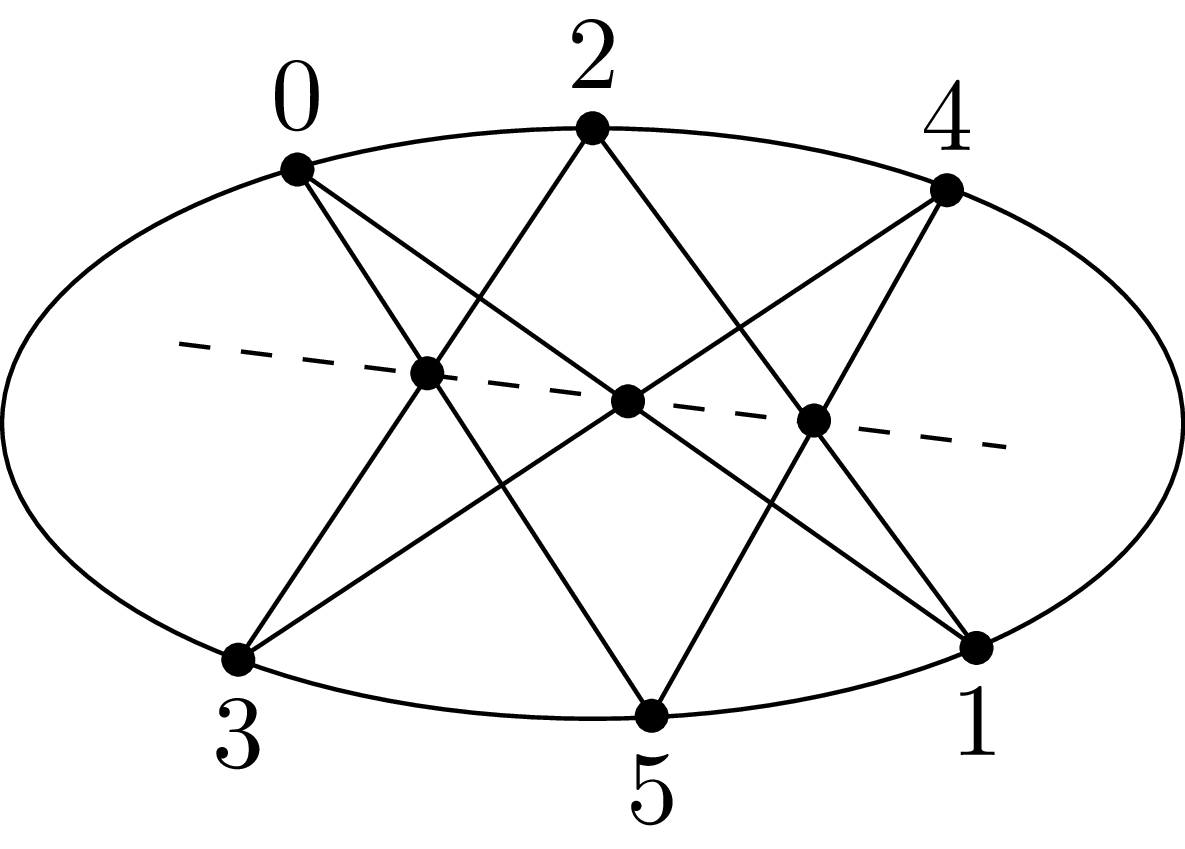
Six points lie on a conic when the points
 $05\cap 23$
,
 $01\cap 34$
, and
 $45\cap 12$
are collinear.

The combined work of Pascal, Braikenridge and Maclaurin [Reference Coxeter and Greitzer5, section 3·8] solved the much simpler version of the Bruxelles Problem for conic curves.
Theorem 1·1 (Pascal, Braikenridge–Maclaurin). Six points labelled 0, 1, 2, 3, 4 and 5 in the plane lie on a conic curve precisely when the three points
 $05\cap 23$
,
 $01\cap 34$
, and
 $45\cap 12$
are collinear, as illustrated in Figure 1.
When the six points are the vertices of a regular hexagon in cyclic order, the intersecting lines in the theorem are parallel and meet on the line at infinity. It is thus natural to interpret problems in synthetic geometry as set in projective space. Projective space was already in use when the Bruxelles Problem was posed but it was not until 1847 that it was given a full modern treatment, in von Staudt’s series of books on the Geometry of Position (1847-1860)Footnote 1. Nevertheless, the modern version of the Bruxelles Problem sets the ten points in projective 3-space,
 $\mathbb{P}^3$
.
Many geometers of the nineteenth century attempted to solve the Bruxelles Problem, including Chasles, Hesse, Serret and Steiner [Reference Turnbull and Young20, footnotes, p. 1]. In his Ausdehnungslehre of 1862 [Reference Grassmann8, section 324], Grassmann gave an elegant solution to the Bruxelles Problem when 3 skew lines,
 $L_0$
,
 $L_1$
, and
 $L_2$
, each contain three of the ten points. In this case, the tenth point x lies on the unique quadric surface containing the lines if the plane
 $xL_0$
containing x and
 $L_0$
meets the line
 $L_1$
in a point that lies on the plane
 $xL_2$
. Grassmann uses the compact notation
 $xL_0L_1L_2x=0$
to describe this situation. Ciliberto and Miranda [Reference Ciliberto and Miranda4] consider many special cases of the Bruxelles Problem, characterising when ten points lie on a quadric using rational normal curves.
The Bruxelles Problem is computationally feasible: the ten points
 $[x_i\;:\;y_i\;:\;z_i\;:\;w_i]$
(
 $i \in \{0,\ldots,9\}$
) lie on a quadric surface precisely when the double Veronese images of the ten points lie on a hypersurface in
 $\mathbb{P}^9$
; that is, when the determinant of the
 $10 \times 10$
matrix
 \begin{align*}N = \left[ \begin{array}{llllllllll} x_0^2 & x_0y_0 & x_0z_0 & x_0w_0 & y_0^2 & y_0z_0 & y_0w_0 & z_0^2 & z_0w_0 & w_0^2 \\x_1^2 & x_1y_1 & x_1z_1 & x_1w_1 & y_1^2 & y_1z_1 & y_1w_1 & z_1^2 & z_1w_1 & w_1^2 \\& & & & & \vdots & & & & \\x_9^2 & x_9y_9 & x_9z_9 & x_9w_9 & y_9^2 & y_9z_9 & y_9w_9 & z_9^2 & z_9w_9 & w_9^2\end{array} \right]\end{align*}
vanishes.
The property that ten points lie on a quadric is invariant under linear change of coordinates. The Fundamental Theorem of Invariant Theory (see Sturmfels [Reference Sturmfels16, theorem 3·2·1]) then implies that the determinant of N can be written as a polynomial in the brackets [abcd], where [abcd] stands for the determinant of the
 $4\times 4$
matrix whose columns consist of the homogeneous coordinates of four points labelled with integers a, b, c and d. Turnbull and Young [Reference Turnbull and Young20] used invariant-theoretic methods to construct a 240-term bracket polynomial that vanishes precisely when the ten points lie on a quadric surface. White [Reference White21] showed that their polynomial can be straightened to a shorter polynomial with 138 terms. Sturmfels and Whiteley [Reference Sturmfels and Whiteley17] proved that every bracket polynomial P admits a bracket monomial, a product of brackets T, so that TP can be Cayley factored: TP can be expressed using a combination of meet and join operations. Though P may not factor directly, a factorisation exists for almost all point configurations, those for which the bracket monomial T does not vanish. Such Cayley expressions using just the meet and join operations immediately provide a synthetic construction to check whether an expression vanishes. Apel and Richter–Gebert ([Reference Apel1] and [Reference Apel and Richter–Gebert2]) gave an explicit algorithm to translate bracket polynomials in
 $\mathbb{P}^2$
into meet and join operations. Their algorithm expresses a bracket polynomial in terms of oriented distance ratios using the Area Principle, popularised by Grünbaum and Shephard [Reference Grünbaum and Shephard10]. One key step in our solution, described in Lemma 4·3 and Remark 4·4, extends these techniques to 3-dimensional space.
1·1. Strategy of the construction
The main step in our construction applies when the degree-4 bracket monomial
 \begin{align*}T = [0123][0145][2345][6789]\end{align*}
does not vanish. This monomial is nonzero precisely when the three lines 01, 23 and 45 are skew and the four points 6, 7, 8 and 9 are not coplanar. In Section 3 we show that ad-hoc methods suffice to solve the Bruxelles Problem when there is a relabelling of the points so that
 $T=0$
.
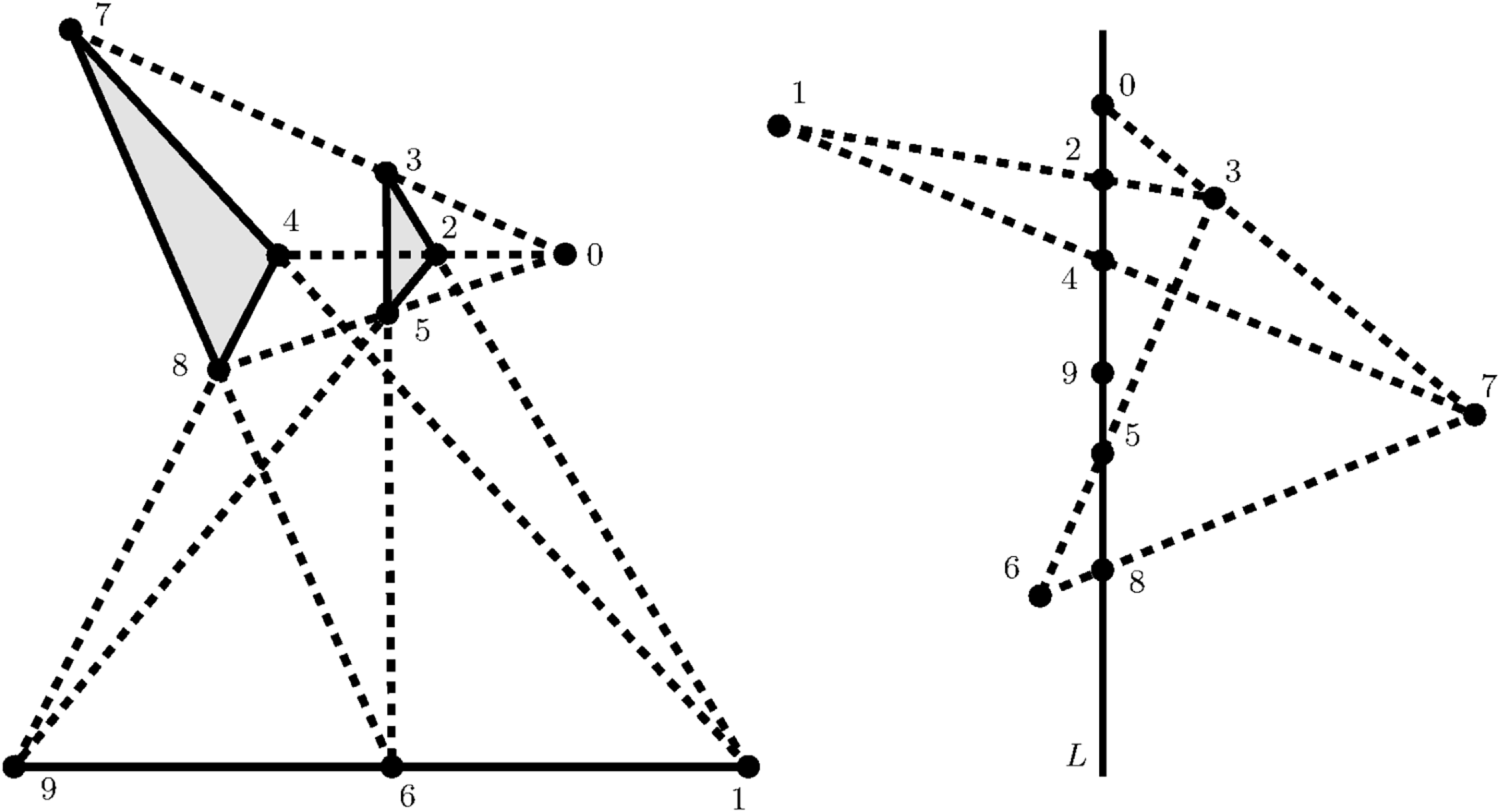
The reader only interested in the case where the ten points lie in linearly general position may skip the argument in Section 3, though it can happen that incidence results that work for points in linearly general position fail for points in special position. For instance, Desargues’s Theorem says that two triangles are in perspective axially (pairs of corresponding edges meet in collinear points) if and only if they are in perspective centrally (lines joining corresponding vertices are coincident), as illustrated on the left side of Figure 2. An incidence version of Desargues’s Theorem might start with ten points
 $0, 1, \ldots, 9$
in
 $\mathbb{P}^2$
and require the triple (1, 6, 9) to be collinear when the triples (1, 2, 3), (1, 4, 7), (0, 2, 4), (2, 5, 9), (3, 5, 6), (0, 3, 7), (0, 5, 8), (4, 8, 9) and (6, 7, 8) are collinear. This formulation is equivalent to Desargues’s Theorem when the two triangles 235 and 478 are in general position; in this case, the triangles are in perspective axially precisely when the triple (1, 6, 9) is collinear. However, this equivalence can break down when the triangles are in special position. Richter–Gebert [Reference Richter–Gebert13, example 1·1] gives an example where the triangles have sides lying on the same line. Pick points 0, 2, 4, 5 and 7 all lying on a line L, and choose the remaining points to lie off L and satisfy the hypotheses. Then the point 9 can be chosen to lie anywhere on L and off
 $\overline{16}$
, producing a counterexample to the incidence formulation, as shown on the right-hand side of Figure 2.
(left) Desargues’s Theorem: the two triangles are in perspective axially from the line
 $\overline{16}$
and centrally from the point 0; (right) The incidence version fails when sides 48 and 25 lie on a line.

Section 4 treats the generic case, where
 $T\neq 0$
. We show that the labels of the first six points can be permuted so that the set
 \begin{align*} \mathcal{S} = \{ [015X][234X], [012X][345X], [024X][135X], [045X][123X] \}\end{align*}
forms a basis for the family of degree-2 functions vanishing on the first six points; here,
 $X = [x\;:\;y\;:\;z\;:\;w]$
is a variable point in
 $\mathbb{P}^3$
and
 \begin{align*}[abcX] = \left| \begin{array}{rrr} a_1& b_1 & c_1\\ a_2 & b_2 & c_2 \\ a_3 & b_3 & c_3 \end{array} \right| w - \left| \begin{array}{rrr} a_1& b_1 & c_1\\ a_2 & b_2 & c_2 \\ a_4 & b_4 & c_4 \end{array} \right| z + \left| \begin{array}{rrr} a_1& b_1 & c_1\\ a_3 & b_3 & c_3 \\ a_4 & b_4 & c_4 \end{array} \right| y - \left| \begin{array}{rrr} a_2& b_2 & c_2\\ a_3 & b_3 & c_3 \\ a_4 & b_4 & c_4 \end{array} \right| x \end{align*}
is a linear polynomial whose zero set is the plane containing points a, b, and c. We use computations in the computer algebra system Macaulay2 (see [Reference Grayson and Stillman9]) to show that such a basis exists.
So the ten points lie on a quadric surface precisely when there is a nonzero polynomial
 \begin{align*} \alpha[015X][234X] +\beta [012X][345X]+\gamma [024X][135X]+\delta [045X][123X]\end{align*}
that evaluates to zero at points 6, 7, 8 and 9. This is equivalent to the existence of a nonzero solution to the linear system
 \begin{align*} M\mathbf{v} = \begin{bmatrix}[0156][2346] & [0126][3456] & [0246][1356] & [0456][1236] \\ [0157][2347] & [0127][3457] & [0247][1357] & [0457][1237] \\ [0158][2348] & [0128][3458] & [0248][1358] & [0458][1238] \\ [0159][2349] & [0129][3459] & [0249][1359] & [0459][1239]\end{bmatrix} \begin{bmatrix} \alpha \\ \beta \\ \gamma \\ \delta \end{bmatrix} = \begin{bmatrix} 0 \\ 0 \\ 0 \\ 0 \end{bmatrix}.\end{align*}
Each column of the
 $4 \times 4$
matrix M corresponds to a point
 $P_i$
in
 $\mathbb{P}^3$
: the ten points lie on a quadric surface when the four test points
 $P_0$
,
 $P_1$
,
 $P_2$
and
 $P_3$
are coplanar. In Section 4·2 we show how the coordinates of each test point can be obtained as the product of a quotient of brackets if we work in an appropriate chart for each test point. Using the extension of the Area Principle to 3-dimensional space, we identify the quotients with points on a line and locate a point on the line corresponding to their product using constructions originally due to von Staudt (and described in Section 2·2). The product points for three coordinates enable us to reconstruct the image
 $Q_i=\tau(P_i)$
of the test point
 $P_i$
under an automorphism
 $\tau$
of
 $\mathbb{P}^3$
, and the coplanarity of these four image points
 $Q_0$
,
 $Q_1$
,
 $Q_2$
and
 $Q_3$
determines whether the original ten points lie on a quadric surface. As required, all the algebraic manipulations and constructions that produce the four image points can be done using only the meet and join operations.
1·2. Plan of the paper
The paper is organised into four additional sections. Section 2 gives important background information. Our solution depends on defining local coordinates on six lines given by extending the edges of a tetrahedron in
 $\mathbb{P}^3$
; the vertices of the tetrahedron are the points labelled 6, 7, 8 and 9, which explains why we required these points to lie in general position. Local coordinates and cross-ratios are reviewed in Section 2·1. We can recover points in
 $\mathbb{P}^3$
from their projections onto (some of) these six lines, a process described in Section 2·3. Section 3 explains how to handle the non-generic cases and reduce to the generic case. Section 4 describes our synthetic construction in the generic case. The arguments in this section involve computations in the Grassmann–Cayley algebra, which is described in Section 2·4. We advertise some open problems and provide suggestions for further reading in the last section.
2. Incidence in projective space
Every algebraic geometer knows that we need to fix 3 distinct points to kill automorphisms of
 $\mathbb{P}^1$
and, more generally, that any
 $n+2$
points in linearly general position in
 $\mathbb{P}^n$
can be sent to any other
 $n+2$
points in linearly general position via a unique automorphism of
 $\mathbb{P}^n$
. This result plays a key role in our solution to the Bruxelles Problem. In this section, we summarise other important background results needed in our construction.
The product construction depends on the choice of an auxiliary point a and line
 $L^\prime$
.

2·1. Cross ratios as local coordinates
We first recall some additional facts about the projective line. After a linear change of coordinates on the underlying two-dimensional space, we can parameterise the line so that three given points – zero, unit, and infinity – are located at
 $p_0=[1\;:\;0]$
,
 $p_1=[1\;:\;1]$
, and
 $p_\infty=[0\;:\;1]$
, respectively. The cross ratio
 $(a,b;\;c,d)$
of any four labelled points on
 $\mathbb{P}^1$
is the point
 $p=\phi(d)$
, where
 $\phi$
is the unique linear automorphism of
 $\mathbb{P}^1$
that sends a to
 $p_\infty$
, b to
 $p_0$
, and c to
 $p_1$
, so that
 $(p_\infty,p_0;\;p_1,p)=p$
. We will identify the point
 $p_x=[1\;:\;x]$
with the parameter value x and this parameter can be recovered using determinants to compute the cross ratio [Reference Richter–Gebert15, lemma 5·5]:
 \begin{align*}(p_\infty,p_0;\; p_1,p_x) = \frac{[p_\infty p_1][p_0 p_x]}{[p_\infty p_x][p_0 p_1]} = \frac{(\!-\!1)(x)}{(\!-\!1)(1)}=x ,\end{align*}
where the notation
 $[\cdot]$
stands for the determinant of the square matrix whose columns are the homogeneous coordinates of the points enclosed by the bracket. The computation of the cross ratio does not depend on the choice of representatives for the points: multiplying any of the points by a constant does not change the cross ratio. Furthermore, the value of the cross ratio is invariant under change of coordinates on the projective line since if
 $A \in GL_2$
,
 $[(Ap_i)(Ap_j)] = \det(A)[p_ip_j]$
. When the four points
 $p_0$
,
 $p_1$
,
 $p_\infty$
and
 $p_x$
lie on an arbitrary line in
 $\mathbb{P}^2$
, we can compute their cross ratio using any point q off the line,
 \begin{align*}(p_\infty,p_0;\; p_1,p_x) = \frac{[p_\infty p_1 q][p_0 p_x q]}{[p_\infty p_x q][p_0 p_1 q]}.\end{align*}
This is easy to check if we choose coordinates so that
 $p_0$
,
 $p_\infty$
and q are the standard basis vectors for the vector space underlying
 $\mathbb{P}^2$
. Similarly, when the points are collinear in
 $\mathbb{P}^3$
and q and r are two distinct points off the line,
 \begin{align*}(p_\infty,p_0;\; p_1,p_x) = \frac{[p_\infty p_1 qr][p_0 p_x qr]}{[p_\infty p_x qr][p_0 p_1 qr]}.\end{align*}
2·2. The product construction
Consider a line L in
 $\mathbb{P}^2$
. After a change of basis on
 $\mathbb{P}^2$
we may assume that L is the line spanned by
 $p_0=[1\;:\;0\;:\;0]$
and
 $p_\infty=[0\;:\;1\;:\;0]$
and the unit on L is
 $p_1=[1\;:\;1\;:\;0]$
. Given a point
 $p_x=[1\;:\;x\;:\;0]$
on L, the map
 $\gamma\;:\; L \rightarrow L$
fixing
 $p_0$
and
 $p_\infty$
and sending
 $p_1$
to
 $p_x$
corresponds to left multiplication by the
 $3\times 3$
diagonal matrix
 $A_x = \text{diag}(1,x,1)$
which sends
 $p_y=[1\;:\;y\;:\;0]$
to
 $p_{xy}=[1\;:\;xy\;:\;0]$
. That is, scaling the unit by x, multiplies
 $p_y$
by x as well. The mathematician von Staudt showed that the map
 $\gamma$
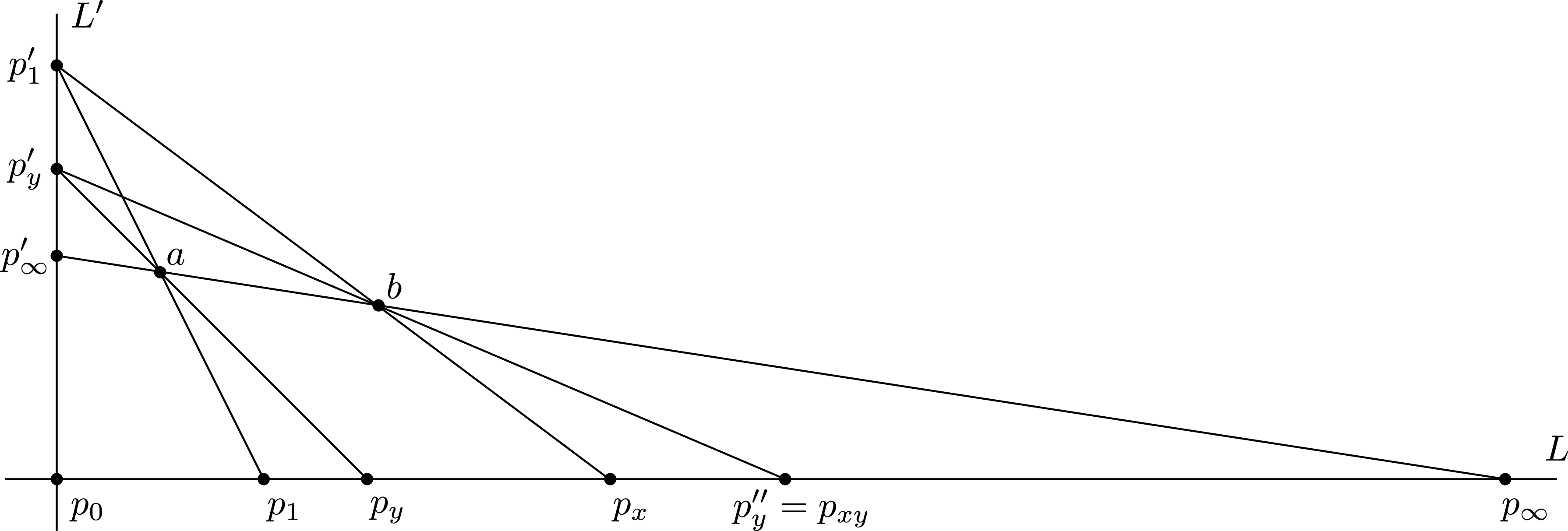
can be achieved by a composition of two maps, each given by projection from a point, as illustrated in Figure 3. We start by picking a point a off L and another line L
′ through
 $p_0$
. Define the points
 $p_0'=p_0$
,
 $p_1'$
,
 $p_y'$
and
 $p_\infty'=p_\infty$
on L
′ to be the projections of
 $p_0$
,
 $p_1$
,
 $p_y$
and
 $p_\infty$
from a onto L
′. Now set b equal to the intersection of the line joining
 $p_1'$
to x with the line joining a and
 $p_\infty$
. Then define the points
 $p_0^{\prime\prime}=p_0$
,
 $p_1^{\prime\prime}$
,
 $p_y^{\prime\prime}$
and
 $p_\infty^{\prime\prime}=p_\infty$
on L to be the projections of
 $p_0'$
,
 $p_1'$
,
 $p_y'$
and
 $p_\infty'$
from b onto L. The projection of L from a onto L
′ followed by the projection of L
′ from b onto L fixes
 $p_0$
and
 $p_\infty$
and sends
 $p_1$
to
 $p_x$
, so the composition equals the map
 $\gamma$
; in particular,
 $p_{y}^{\prime\prime}=p_{xy}$
is constructed from
 $p_0$
,
 $p_1$
,
 $p_\infty$
,
 $p_x$
and
 $p_y$
in this manner. Though we chose a convenient basis to describe the construction, the construction of the point corresponding to xy from the points corresponding to x and y works for any line L in
 $\mathbb{P}^2$
, and even for lines in higher-dimensional projective spaces. Note that this product construction only depends on incidence relations and the positions of the points
 $p_0$
,
 $p_1$
and
 $p_\infty$
on L.
Reversing the order of the construction in an appropriate way gives a construction of
 $p_{1/x}$
from
 $p_{x}$
. First we draw a new line L
′ through
 $p_0$
. Then we pick a point b off
 $L \cup L'$
and draw lines
 $p_{\infty}b$
,
 $p_x b$
and
 $p_1b$
. We draw the line
 $(p_xb\cap L')p_1$
and let a denote the intersection of this line and
 $p_\infty b$
. Then we draw
 $(p_1b\cap L')a$
, which intersects L at the point
 $p_{1/x}$
. This construction works fine if
 $x=0$
or
 $x=\infty$
: if
 $x=0$
it produces
 $p_\infty$
and if
 $x=\infty$
it produces
 $p_0$
.
2·3. Recovering points from local coordinates
Now we focus on 3-dimensional projective space. After a change of coordinates on the underlying vector space, any five points in linearly general position in
 $\mathbb{P}^3$
(no four on a plane) are located at
 $E_0=[1\;:\;0\;:\;0\;:\;0]$
,
 $E_1=[0\;:\;1\;:\;0\;:\;0]$
,
 $E_2=[0\;:\;0\;:\;1\;:\;0]$
,
 $E_3=[0\;:\;0\;:\;0\;:\;1]$
and
 $\mathbf{1}=[1\;:\;1:1\;:\;1]$
. If v is a nonzero vector in four-dimensional space, write
 $\langle v \rangle$
for the point in
 $\mathbb{P}^3$
corresponding to the 1-dimensional subspace containing v. Then the point
 $E_i = \langle e_i \rangle$
corresponds to the standard basis vector
 $e_i$
and
 $\mathbf{1} = \langle e_0+e_1+e_2+e_3 \rangle$
. When
 $i\lt j$
we take
 $E_i$
and
 $E_j$
as the points zero and infinity on
 $E_iE_j$
. Define
 $\mathbf{1}_{ij}$
to be the point
 $\langle e_i+e_j \rangle$
on the line
 $E_iE_j$
;
 $\mathbf{1}_{ij}$
serves as the unit on
 $E_iE_j$
.
The unit points on the lines
 $E_iE_j$
are consistently determined by
 $\mathbf{1}$
through an incidence construction. If
 $\{i,j,k,\ell\} = \{0,1,2,3\}$
, define the projection
 $\pi_{ij}\;:\; \mathbb{P}^3 \dashrightarrow E_iE_j$
sending P to the intersection of the line
 $E_iE_j$
with the plane
 $E_k E_\ell P$
containing
 $E_k$
,
 $E_\ell$
and P. The projection morphism
 $\pi_{ij}$
is defined off the line
 $E_kE_\ell$
. The point
 $P=[x_0\;:\;x_1\;:\;x_2\;:\;x_3] = \langle x_0e_0+x_1e_1+x_2e_2+x_3e_3 \rangle$
is sent by the projection
 $\pi_{ij}$
to
 $\pi_{ij}(P) = \langle x_ie_i + x_je_j\rangle$
. In particular,
 $\pi_{ij}(\mathbf{1}) = \mathbf{1}_{ij}$
. If
 $i\lt j$
, then
 $\pi_{ij}(P)$
is the point on
 $E_iE_j$
corresponding to the parameter value
 $x_j/x_i$
. In this way, the locations of the five points
 $E_0$
,
 $E_1$
,
 $E_2$
,
 $E_3$
, and
 $\mathbf{1}$
in
 $\mathbb{P}^3$
determine units and local parameters on all six lines
 $E_iE_j$
.
For
 $0\leq i \leq 3$
, let
 $U_i$
stand for the chart
 $\{[x_0\;:\;x_1\;:\;x_2\;:\;x_3] \in \mathbb{P}^3:\, x_i \neq 0\} \cong K^3$
. The four charts
 $U_i$
cover
 $\mathbb{P}^3$
. We say that the chart
 $U_i$
is spanned by the lines
 $E_{i}E_{j}$
with
 $j\neq i$
and that the line
 $E_iE_j$
is part of a spanning set for
 $U_i$
. We can use projections to determine if a point lies in a chart: the point P lies in
 $U_i$
if and only if the projections
 $\pi_{ij}(P)$
exist and are not equal to the infinity point for all three lines
 $E_iE_j$
spanning
 $U_i$
. Moreover, given the projections of a point P onto the lines spanning a chart
 $U_i$
, we can recover P by intersecting three transverse planes: if
 $\{i,j,k,\ell\}=\{0,1,2,3\}$
and P lies in
 $U_i$
then
 \begin{align*}P = \pi_{ij}(P)E_kE_\ell \cap\pi_{ik}(P)E_jE_\ell \cap\pi_{i\ell}(P)E_jE_k.\end{align*}
2·4. The Grassmann–Cayley algebra
The Grassmann–Cayley algebra provides an algebraic and computational way to work with the intersection and span of linear spaces; for details, see Sturmfels [Reference Sturmfels16, section 3·3]. Given a d-dimensional vector space V, the meet and join operations define product structures on the exterior algebra
 $\oplus_{k=0}^d \bigwedge^k V$
. We say that an element is a k-extensor if it is the wedge product of k vectors. The two operations are linear, so it suffices to define them for products of extensors. We warn the reader that the usual notation for meets (
 $\wedge$
) and joins (
 $\vee$
) conflicts with the wedge product: we write
 $A = a_1\vee a_2 \vee \cdots a_k$
for the wedge product of k vectors
 $a_i$
and abbreviate this expression as
 $A =a_1a_2\cdots a_k$
. A nonzero extensor
 $A=a_1a_2\cdots a_k$
involves vectors
 $a_1,\ldots,a_k$
that span a k-dimensional vector space
 $\overline{A} = \{v \in V\;:\; a_1a_2\cdots a_kv=0\} $
. Conversely, any k-dimensional vector space
 $\bar{A}$
determines (up to scalar multiple) an extensor A given by the wedge product of a basis for
 $\bar{A}$
. If
 $A=a_1a_2\cdots a_j$
is a j-extensor and
 $B=b_1b_2\cdots b_k$
is a k-extensor, then their join is a
 $(j+k)$
-extensor
 $A \vee B = a_1a_2\cdots a_jb_1b_2\cdots b_k$
. If the join
 $A \vee B$
is nonzero, then the vectors
 $a_1,\ldots,a_j,b_1,\ldots,b_k$
are linearly independent and
 $\overline{A\vee B}$
equals
 $\overline{A}+\overline{B}$
, the span of
 $\overline{A}$
and
 $\overline{B}$
. Fix a basis
 $e_1,\ldots,e_d$
for the vector space V and identify
 $\bigwedge^d V$
with the 1-dimensional vector space spanned by this basis, sending
 $e_1\cdots e_d$
to 1. Then any d-extensor
 $a_1\cdots a_d$
is identified with the determinant
 $[a_1\cdots a_d]$
since
 $a_1\cdots a_d = [a_1\cdots a_d]e_1\cdots e_d$
.
The meet
 $A \wedge B$
of
 $A=a_1a_2\cdots a_j$
and
 $B=b_1b_2\cdots b_k$
with
 $j+k \geq d$
is
 \begin{align*} A \wedge B = \sum_\sigma \text{sign}(\sigma) [a_{\sigma(1)}\cdots a_{\sigma(d-k)}b_1\cdots b_k]a_{\sigma(d-k+1)}\cdots a_{\sigma(j)},\end{align*}
where the sum is over all
 $(d-k,j-(d-k))$
-split shuffles, i.e. permutations of
 $\{1,\ldots, j\}$
with
 $\sigma(1)\lt\cdots\lt\sigma(d-k)$
and
 $\sigma(d-k+1)\lt\ldots\lt\sigma_d$
. The meet
 $A \wedge B$
is defined to be zero if
 $j+k \lt d$
. The meet of two extensors is an extensor and we have
 $A\wedge B$
is nonzero if and only if
 $\overline{A}+\overline{B}=V$
. In that case, the meet corresponds to the intersection of subspaces,
 $\overline{A \wedge B} = \overline{A} \cap \overline{B}$
.
If p, q and r are points in a projective space, then the join pq corresponds to the line through p and q (
 $pq=0$
if
 $p=q$
). The join pqr corresponds to the plane containing p, q and r (
 $pqr=0$
if the points lie on a line). In
 $\mathbb{P}^2$
the meet operator can be used to give an explicit description of the point of intersection of two lines,
 \begin{align*} pq \wedge rs = [prs]q-[qrs]p\end{align*}
and in
 $\mathbb{P}^3$
we can find explicit expressions for the intersection of a line with a plane,
 \begin{align*}pq\wedge rst =[prst]q - [qrst]p,\end{align*}
and the intersection of two planes,
 \begin{align*} pqr\wedge stu = [pstu]qr - [qstu]pr + [rstu]pq.\end{align*}
3. Geometric reductions
In this section we handle several cases where the geometry of the ten points is special enough to solve the Bruxelles Problem using ad-hoc techniques.
If two of the ten points agree then two of the rows in the constraint matrix N agree and so
 $\text{det}(N)=0$
and the points lie on a quadric. If four of the ten points lie on a line, then the constraints imposed by three of the points force the fourth point constraint to be satisfied, since any quadric that contains three collinear points must contain the entire line. If all ten points lie on the union of two planes then the points lie on a degenerate quadric. If six of the points lie on a plane then we can use Pascal’s Theorem to check whether the six points lie on a conic and this happens precisely when all ten points lie on a quadric. From now on we assume that all ten points are distinct and do not lie on the union of two planes, no four points are collinear, and no six of the points lie on a plane. Now we leverage these assumptions to further constrain the geometry of the ten points.
Lemma 3·1 For each set
 $\{a, b, c, d, e, f\}$
of six of our ten points, at least one of the following conditions hold:
-
(i) we can partition the six points into three disjoint pairs that generate skew lines; or
-
(ii) five of the six points are coplanar and the sixth point lies off the plane.
Proof. Suppose that (i) fails: every partition of the six points into three sets of two points fails to generate skew lines. In particular, two of the lines ab, cd and ef meet. Without loss of generality, ab meets cd, so that the four points a, b, c and d are coplanar. By our standing assumptions, points e and f cannot both lie on the plane abcd.
Now we argue that (ii) holds. We first treat the generic case, where no three of a, b, c and d are collinear. Consider one of the six lines joining two of the four points, cd, say. Taking the line ab joining the other two points, and two lines ce and df joining the points spanning cd to e and f, we have three lines, ab, ce and df. By assumption, two of these three lines must meet. If the line ab meets ce or df then e or f must lie on abcd and (ii) holds. Otherwise, ce and df must meet. Then the points c, d, e and f are coplanar, so ef meets the line cd. Applying this argument to each of the six lines, we find that either (ii) holds or the line ef meets each of the six lines. But the line ef meets the plane abcd in a point and no point lies on all six lines! We conclude that (ii) holds when no three of the four points are collinear.
Now we treat the collinear case. Without loss of generality, assume a, b and c are collinear and d lies off this line. Now consider the three lines ae, bf and cd. Since (i) fails, two of the three lines must meet but each possibility forces five of the six points to be coplanar. If cd meets either ae or bf then e or f lies on abcd. If ae meets bf then a, b, c, e and f are coplanar (and d lies off this plane). This establishes (ii) in the collinear case.
Theorem 3·2. Under our standing assumptions, four of our ten points are in general position and the other six can be partitioned into three disjoint pairs spanning mutually skew lines.
Proof. By our standing assumptions, among our ten points there exist four points
 $\alpha$
,
 $\beta$
,
 $\gamma$
,
 $\delta$
in general position, otherwise all the points lie on a plane. Apply Lemma 3·1 to the set
 $\{a, b, c, d, e, f\}$
of remaining points. Our theorem follows immediately if (i) holds so we can assume that (ii) holds: five of the six points are coplanar. Without loss of generality, assume that f lies off the plane abcde.
Since the four points lie in general position, we can replace one of the four general points with a and still have four points in general position; without loss of generality assume a,
 $\beta$
,
 $\gamma$
and
 $\delta$
lie in general position. Apply Lemma 3·1 again, this time to the set of points
 $\{\alpha, b, c, d, e, f\}$
. Our theorem follows immediately if (i) holds so we can assume that (ii) holds: five of the six points
 $\alpha$
, b, c, d, e and f are coplanar. Since f lies off the plane bcde, the plane would have to be
 ${\alpha}bcde$
. Then the six points
 $\alpha$
, a, b, c, d and e are coplanar, violating our standing assumptions. We conclude that four of the ten points are in general position and three pairs of the remaining points generate skew lines.
Remark 3·3. The points 6, 7, 8 and 9 are in general linear position precisely when
 $[6789]\neq 0$
and the skewness of the lines 01, 23, and 45 is characterised by
 $[0123][0145][2345]\neq 0$
. So Theorem 3·2 reduces the Bruxelles Problem to the case where, after relabelling the points,
 $T = [0123][0145][2345][6789]$
is nonzero.
4. The generic case
In this section, we describe an algorithm to decide whether the ten points 0, 1,
 $\ldots$
, 9 lie on a quadric surface. In Section 3, we reduced the problem to considering ten points that satisfy the genericity conditions: all ten points are distinct; all ten points do not lie on the union of two planes; no four of the ten points are collinear; and no six points lie on a plane. Under these assumptions, we apply Theorem 3·2 and relabel the points so that the lines 01, 23 and 45 are mutually skew, and the points 6, 7, 8 and 9 are in general position (not contained in a plane).
4·1. A family of quadrics
We focus on the quadric surfaces that pass through the six points 0, 1, 2, 3, 4 and 5. We claim that the assumption that 01, 23 and 45 are skew lines implies that the six points impose independent conditions on quadrics, so there is a
 $\mathbb{P}^3$
of quadrics through all six points. Since the points 0, 1, 2 and 3 are in general position, we can apply a projective linear transformation to the points to put them at
 $[1\;:\;0\;:\;0\;:\;0]$
,
 $[0\;:\;1\;:\;0\;:\;0]$
,
 $[0\;:\;0\;:\;1\;:\;0]$
, and
 $[0\;:\;0\;:\;0\;:\;1]$
. Suppose that point 4 is at
 $[x_4\;:\;y_4\;:\;z_4\;:\;w_4]$
and point 5 is at
 $[x_5\;:\;y_5\;:\;z_5\;:\;w_5]$
. Representing a general quadric with the equation
 \begin{align*}ax^2 + bxy + cxz + dxw + ey^2 + fyz + gyw + hz^2 + izw + jw^2 =0,\end{align*}
we see that the quadrics passing through points 0, 1, 2, and 3 have
 $a=e=h=j=0$
and the points 4 and 5 impose dependent conditions when
 \begin{align*}\text{Rank}\left( \begin{bmatrix} x_4y_4 & x_4z_4 & x_4w_4 & y_4z_4 & y_4w_4 & z_4w_4 \\x_5y_5 & x_5z_5 & x_5w_5 & y_5z_5 & y_5w_5 & z_5w_5 \end{bmatrix}\right) \leq 1.\end{align*}
This occurs when all the
 $2 \times 2$
minors of this matrix vanish. Macaulay2 can be used to find the primary decomposition of the ideal generated by the minors. The primary components correspond to one of the following conditions: points 4 and 5 are equal; point 4 or 5 equals one of points 0, 1, 2, or 3; or the points 4 and 5 are collinear with two of the four points 0, 1, 2 and 3. All of these situations violate our assumptions for this section, so we conclude that the six points 0, 1, 2, 3, 4 and 5 impose independent conditions on quadrics and the set of quadrics passing through the six points forms a
 $\mathbb{P}^3$
.
We now find a basis for the quadrics passing through the first six points. Write [abcX] for the determinant of the
 $4 \times 4$
matrix whose columns are the points a, b, c, and the variable point
 $X = [x\;:\;y\;:\;z\;:\;w]$
so that
 $[abcX]=0$
is the equation of the plane through points a, b and c. We pick a set of four reducible quadrics
 \begin{align*} \mathcal{S} = \{ [015X][234X], [012X][345X], [024X][135X], [045X][123X] \}\end{align*}
through the points 0, …, 5, and investigate when these span the space of quadrics through all six points. It is easier to check the equivalent condition for these four polynomials to be linearly independent. Working in the ring
 $\mathbb{Q}[x_4,y_4,z_4,w_4,x_5,y_5,z_5,w_5][x,y,z,w]$
we compute the
 $4 \times 10$
matrix whose entries in each column are the coefficients of the degree-2 monomials in x, y, z, and w appearing in the polynomials in
 $\mathcal{S}$
. The polynomials in
 $\mathcal{S}$
are linearly dependent when all the
 $4 \times 4$
minors of this matrix vanish. Using Macaulay2, we find that the ideal generated by these minors is a primary ideal and its minimal prime ideal is generated by
 \begin{align*} Q = -x_5y_4z_5w_4 + x_4y_5z_5w_4+ x_5y_4z_4w_5 - x_4y_4z_5w_5. \end{align*}
We give an incidence interpretation of the condition
 $Q=0$
.
Lemma 4·1. The expression Q is equal to the expansion of the bracket binomial
 \begin{align*} [0125][0234][1345] - [0124][2345][0135]\end{align*}
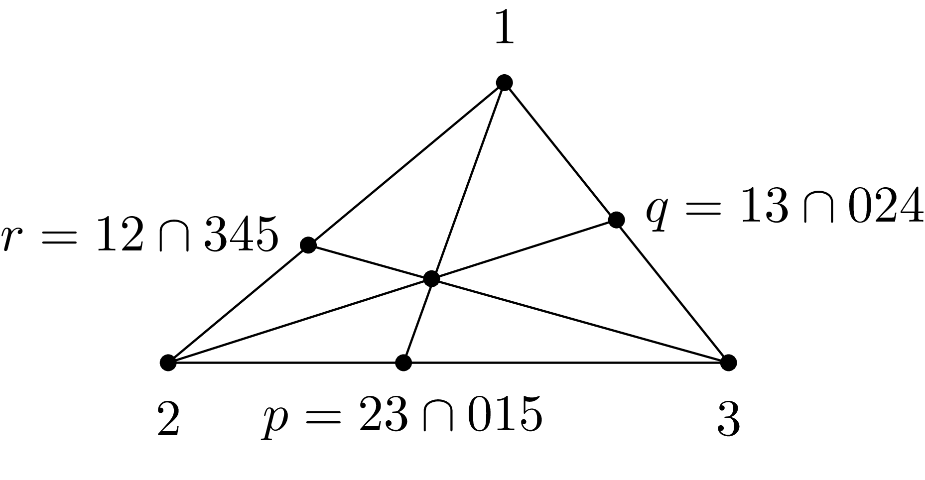
and both vanish precisely when an incidence condition reminiscent of Ceva’s Theorem holds: if we set
 $p = 23 \cap 015$
equal to the intersection of the line 23 and the plane 015,
 $q=13\cap 024$
and
 $r = 12 \cap 345$
then the condition
 $Q=0$
requires that the lines 1p, 2q, and 3r meet in a common point, as shown in Figure 4.
An incidence interpretation of
 $Q=0$
.

Proof. A direct computation shows that the bracket polynomial equals Q. Taking the meet of 23 with 015 gives an explicit description of
 $p=[2015]3-[3015]2 = [0125]3 - [0135]2$
as a point on the line 23. Similarly,
 $q = -[0124]3-[0234]1$
and
 $r=[1345]2-[2345]1$
. The lines 1p and 2q should meet because they are in the plane 123 but their point of intersection can be difficult to compute directly in the Grassmann–Cayley algebra. Instead, we cone over the point 0 (which lies off the plane 123 since 01 and 23 are skew) and intersect the planes 01p and 02q, giving a line containing 0 and the intersection point of 1p and 2q. Taking the meet of 01p and 02q gives
 $-[102q]0p +[p02q]01$
. The line corresponding to this element meets the line 3r only if the line 3r contains the intersection point of 1p and 2q. Taking the meet of the line with 3r gives a bracket polynomial
 $-[102q][0p3r]+[p02q][013r]$
which must vanish precisely when 1p, 2q, and 3r are coincident. Substituting for p, q, and r, we obtain
 \begin{align*} -[102q][0p3r]+[p02q][013r] =[0123]^2 Q. \end{align*}
Since 01 and 23 are skew, [0123] is nonzero, so
 $Q=0$
characterises when 1p, 2q and 3r are coincident.
It may happen that the expression Q is zero and so the four quadrics in
 $\mathcal{S}$
are linearly dependent. We get around this difficulty by permuting the point labels. Given a permutation
 $\sigma$
of the set
 $\{0,1,2,3,4,5\}$
, we set
 $ \sigma([abcd]) = [\sigma(a)\sigma(b)\sigma(c)\sigma(d)]$
and extend this action to a ring homomorphism on the bracket algebra (the polynomial ring on the brackets modulo the ideal generated by the relations among the brackets, the Grassmann–Plücker relations, which can be obtained in Macaulay2 using the Grassmannian command). Now we form the ideal
 $I = (\sigma(Q)\;:\; \sigma \in \mathbb{S}_6)$
, generated by all the permutations applied to the expression Q, thought of as an element of the bracket algebra. This ideal contains the polynomial [0123][0145][2345], which vanishes only when two of the three lines 01, 23 and 45 meet. Since the lines are skew,
 $\sigma(Q)\neq 0$
for some
 $\sigma$
and we can identify the permutation
 $\sigma$
using the incidence interpretation given in Lemma 4·1. Relabelling each of the six points
 $\sigma(i)$
with the label i, we find that
 $Q \neq 0$
and the polynomials in
 $\mathcal{S}$
are a basis for the space of all quadrics that pass through the six points.
Remark 4·2. We note that after relabelling, three lines corresponding to a partition of the 6 points into 3 pairs (generating the lines) are skew but these three lines may not be 01, 23 and 45. We will not need these skew lines in what follows.
Searching for a quadric through all ten points requires us to find a polynomial of the form
 \begin{align*}\alpha [015X][234X]+\beta [012X][345X]+\gamma [024X][135X]+\delta [045X][123X]\end{align*}
that vanishes at
 $X = 6$
, 7, 8 and 9. So we are led to solve a system
 \begin{align*} M\mathbf{v} = \begin{bmatrix}[0156][2346] & [0126][3456] & [0246][1356] & [0456][1236] \\ [0157][2347] & [0127][3457] & [0247][1357] & [0457][1237] \\ [0158][2348] & [0128][3458] & [0248][1358] & [0458][1238] \\ [0159][2349] & [0129][3459] & [0249][1359] & [0459][1239]\end{bmatrix} \begin{bmatrix} \alpha \\ \beta \\ \gamma \\ \delta \end{bmatrix} = \begin{bmatrix} 0 \\ 0 \\ 0 \\ 0 \end{bmatrix}.\end{align*}
We can assume that none of the columns of M are zero; otherwise, the points 6, 7, 8 and 9 lie on a union of two planes, each passing through 3 of the remaining points, so the ten points lie on a union of two planes. There is a nice connection between the two matrices M and N and the polynomial Q:
 $\det(M)=Q\det(N)$
modulo the Plücker relations (that is, in the bracket algebra). It is not clear whether this is a coincidence or an indication of some more general result.
The system
 $M\mathbf{v}=\mathbf{0}$
has a nonzero solution precisely when
 $\det M = 0$
, that is, when the four test points
 $P_1$
,
 $P_2$
,
 $P_3$
and
 $P_4$
, whose coordinates are given by the columns of M, are coplanar. Rather than constructing these four points, we construct their images under an invertible projective transformation using meet and join operations.
4·2. Constructing the test points
We construct the images
 $Q_i=\tau(P_i)$
of the four columns
 $P_1$
,
 $P_2$
,
 $P_3$
and
 $P_4$
of M under an appropriate invertible projective transformation
 $\tau\;:\; \mathbb{P}^3 \rightarrow \mathbb{P}^3$
. The four points 6, 7, 8 and 9 are in linearly general position and span a
 $\mathbb{P}^3$
. Choose vectors so that points 6, 7, 8 and 9 equal
 $\langle v_6\rangle$
,
 $\langle v_7\rangle$
,
 $\langle v_8\rangle$
and
 $\langle v_9\rangle$
, respectively, and then set
 $u = \langle v_6+v_7+v_8+v_9\rangle$
. The
 $\mathbb{P}^3$
containing the ten original points is not the same as the
 $\mathbb{P}^3$
spanned by the columns of M, though they are isomorphic. The isomorphism
 $\tau$
between the two
 $\mathbb{P}^3$
’s is determined by sending
 $E_0$
,
 $E_1$
,
 $E_2$
,
 $E_3$
in the
 $\mathbb{P}^3$
generated by the columns of M to the points 6, 7, 8, 9. This map sends the unit point
 $\mathbf{1}$
to u.
As an example of the construction method, consider
 $P_1$
, the first column of M. The point
 $P_1$
lies in some chart of
 $\mathbb{P}^3$
; for illustrative purposes, we suppose that
 $P_1$
lies in
 $U_0$
. Dividing all the coordinates of
 $P_1$
by the coordinate in the
 $0\,{{th}}$
position, we get an affine representative for
 $P_1$
,
 \begin{align*} \left[1\;:\; \frac{[0157]}{[0156]}\frac{[2347]}{[2346]}\;:\; \frac{[0158][2348]}{[0156][2346]}\;:\;\frac{[0159][2349]}{[0156][2346]} \right].\end{align*}
Now we focus on the second coordinate of this representation of
 $P_1$
. Viewing the coordinate as the product of two fractions, we are inspired to construct a point on a line whose local coordinate is a given ratio of brackets sharing three common entries.
Lemma 4·3. If
 $0 \leq a \lt b \lt c \leq 5$
and
 $6 \leq d \lt e \leq 9$
then the point
 $p = de \wedge abc = [dabc]e - [eabc]d = [abce]d-[abcd]e$
corresponds to the local parameter value
 $-[abcd]/[abce]$
on the line de.
Proof. The expression for p in terms of d and e follows directly from the definition of the meet operation. The local parameter value can be recovered using the cross product. The point
 $d = \langle v_d \rangle$
serves as zero and the point
 $e = \langle v_e \rangle$
serves as infinity on the line de. The unit on de is
 $de\wedge fgu$
, where
 $\{d,e,f,g\} = \{6,7,8,9\}$
and
 $u=\langle v_6+v_7+v_8+v_9 \rangle = \langle v_d+v_e+v_f+v_g \rangle$
. Computing,
 $v_dv_e\wedge v_fv_gv_u = [v_dv_fv_gv_u]v_e - [v_ev_fv_gv_u]v_d = [v_dv_fv_gv_e]v_e-[v_ev_fv_gv_d]v_d = [v_dv_ev_fv_g](v_d+v_e)$
, so the unit
 $\mathbf{1}_{de}$
on de is
 $\langle [v_dv_ev_fv_g](v_e+v_d) \rangle = \langle v_d+v_e\rangle$
. The cross ratio
 $(\mathbf{\infty}_{de},\mathbf{0}_{de};\; \mathbf{1}_{de}, p)$
equals the local coordinate of the point p on de:
 \begin{align*} \begin{array}{lll} (\mathbf{\infty}_{de},\mathbf{0}_{de};\; \mathbf{1}_{de}, p) &= &\dfrac{[e(d+e)fg][dpfg]}{[epfg][d(d+e)fg]} \\[11pt] & = & \dfrac{[edfg][dpfg]}{[epfg][defg]} \\[11pt] & = & \dfrac{[edfg][d([abce]d-[abcd]e)fg]}{[e([abce]d-[abcd]e)fg][defg]}\\[11pt] & = & - \dfrac{[edfg][abcd][defg]}{[abce][edfg][defg]}\\[11pt] & = & - \dfrac{[abcd]}{[abce]}.\end{array}\end{align*}
Remark 4·4. We can also find a point q on de with local parameter value
 $-[abce]/[abcd]$
. We just apply the construction of
 $p_{1/x}$
from
 $p_x$
given in Section 2·2 to the point p in Lemma 4·3.
Using this remark, let
 $p_x = 67 \wedge 015$
be the point on the line 67 with local coordinate
 $x = -[0156]/[0157]$
and construct
 $q_x = p_{1/x}$
. Also let
 $p_y=67 \wedge 345$
be the point with local coordinate
 $y=-[2346]/[2347]$
and construct
 $q_y=p_{1/y}$
. We use the product construction from Section 2·2 on the line 67 to produce a point
 $Q_{67}$
corresponding to the local parameter
 $(\frac{1}{x})(\frac{1}{y}) = [0157][2347]/[0156][2346]$
on the line 67. Similarly, we construct the point
 $Q_{68}$
corresponding to local parameter
 $[0158][2348]/[0156][2346]$
on the line 68. Finally, we construct the point
 $Q_{69}$
corresponding to local parameter
 $[0159][2349]/[0156][2346]$
on the line 69. Now we construct the point
 \begin{align*}Q_1 = Q_{67}89 \cap Q_{68}79 \cap Q_{69}78.\end{align*}
This is the image of
 $P_1$
under the isomorphism
 $\tau$
of
 $\mathbb{P}^3$
, as described in Section 2·3.
The same construction can be applied to the other columns of M to construct the points
 $Q_2$
,
 $Q_3$
and
 $Q_4$
that are the images under
 $\tau$
of
 $P_2$
,
 $P_3$
and
 $P_4$
. The four columns of M are linearly dependent precisely when the four points
 $Q_1$
,
 $Q_2$
,
 $Q_3$
and
 $Q_4$
are coplanar. It follows that the ten original points lie on a quadric surface precisely when the four constructed points
 $Q_1$
,
 $Q_2$
,
 $Q_3$
and
 $Q_4$
are coplanar.
5. Open problems and further reading
Recently, Traves and Wehlau [Reference Traves and Wehlau19] devised a synthetic method to check whether ten points lie on a plane cubic curve. The construction finds two degree-4 curves, each the union of two conics, whose intersection contains the ten points. The Cayley–Bacharach Theorem, beautifully described by Eisenbud, Green and Harris [Reference Eisenbud, Green and Harris6], implies that ten points lie on a cubic precisely when the residual set of six points lies on a conic. Unfortunately, it is not possible to precisely locate all six residual points using a purely synthetic construction; however, synthetic methods still suffice to check whether the six points lie on a conic. See the paper for details. Traves [Reference Traves18] also describes how Grassmann’s methods can be used to determine whether ten points lie on a plane cubic, and solves other synthetic geometry problems involving cubic and conic curves.
Pascal’s Theorem gives rise to a straightedge construction that finds the second point of intersection of a line and a conic (see Construction 1 in Traves and Wehlau [Reference Traves and Wehlau19]). Specifically, given five points
 $p_0, \ldots, p_4$
determining a conic C and a line L through one of the five points, we can construct the second point of
 $L\cap C$
. We can generalise this construction to a quadric hypersurface Q in
 $\mathbb{P}^3$
. If Q contains skew lines
 $L_1$
,
 $L_2$
, and
 $L_3$
and line L meets Q at point p lying off all three lines then we can find another point on
 $L \cap Q$
. First construct a transversal to
 $L_1$
,
 $L_2$
and
 $L_3$
by taking a point t on
 $L_1$
and joining it to the intersection of the plane
 $tL_2$
and the line
 $L_3$
. Pick another point x on the transversal that lies off
 $L_1$
,
 $L_2$
and
 $L_3$
. Then the plane xL contains L and five points on the quadric: x, p, and the three points where the lines
 $L_i$
meet xL. Applying the construction from Pascal’s Theorem, we can find the second point of intersection of L with the conic
 $Q \cap xL$
, as desired. If the point p lies on
 $L_1$
, say, then we only get four points on the conic
 $Q \cap xL$
but it is easy to find more. Just compute another transversal to the three lines and construct the intersection of the new transversal with the plane xL. Constructing transversals also allows us to generalise the construction to the case where we are only given two lines,
 $L_1$
and
 $L_2$
, and three additional points
 $p_0$
,
 $p_1$
and
 $p_3$
lying on Q. Just construct lines joining
 $p_i$
to
 $p_iL_1 \cap L_2$
for
 $i \in \{1,2,3\}$
, which all lie on Q, and apply the construction above using these three lines.
Open problem 5·1. Suppose that one line
 $L_1$
and six points
 $P_1,\ldots,P_6$
in
 $\mathbb{P}^3$
lie on a unique quadric Q. Given a second line L through
 $P_1$
, find a synthetic construction of the second point of intersection of L with Q.
Open problem 5·2. Suppose that nine points
 $P_1,\ldots,P_9$
in
 $\mathbb{P}^3$
lie on a unique quadric Q. Given a second line L through
 $P_1$
, find a synthetic construction of the second point of intersection of L with Q.
Ciliberto and Miranda [Reference Ciliberto and Miranda4] investigate particular instances under which ten points lie on a quadric surface in
 $\mathbb{P}^3$
. For example, they note that if the ten points are broken into two groups of five, then there are rational normal curves through each group and these meet in five points precisely when the ten points lie on a quadric surface (see Ciliberto and Miranda [Reference Ciliberto and Miranda4, proposition 7]). Caminata and Schaffler [Reference Caminata and Schaffler3] gave synthetic conditions for
 $d+4$
points to lie on a rational normal curve of degree d in
 $\mathbb{P}^d$
. Ciliberto and Miranda [Reference Ciliberto and Miranda4, theorem 3] simplified the conditions: the points lie on a rational normal curve precisely when both:
-
(1) the projection from one of the points
 $p_i$
to a
$\mathbb{P}^{d-1}$
applied to the remaining points gives
$d+3$
points on a rational normal curve; and
-
(2) the projection from the span of
$d-2$
points (distinct from
$p_i$
) to a
$\mathbb{P}^2$
applied to the remaining points gives six points lying on a conic.


Ciliberto and Miranda describe another remarkable result, originally due to Richmond [Reference Richmond12], but rediscovered by both Segre and Brown.
Theorem 5·3 (Richmond-Segre-Brown). Five labelled lines
 $L_1,\ldots,L_5$
lie on a quadric surface in
 $\mathbb{P}^4$
precisely when the five points
 $R_i = L_i\wedge(L_{i-1}L_{i+1})$
(indices taken modulo 5) lie on a hyperplane.
There is an infinite family of geometric questions of this form; here are two open problems along these lines.
Open problem 5·4. When do seven lines in
 $\mathbb{P}^5$
lie on a quadric hypersurface?
Open problem 5·5. When does a point in
 $\mathbb{P}^6$
lie on the unique quadric hypersurface containing nine fixed lines?
We can also generalise by degree rather than dimension.
Open problem 5·6. Produce a synthetic construction that checks when twenty points in 3-space lie on a cubic surface.
This problem is similar to a result described by Hartshorne [Reference Hartshorne11, remark 4·9·1]: five skew lines in
 $\mathbb{P}^3$
lie on a cubic surface if and only if there exists another line meeting all five lines. Sturmfels [Reference Sturmfels16, theorem 3·4·7] describes a result due to Neil White that characterises when there is a transversal to five general lines in terms of the vanishing of a
 $5 \times 5$
determinant of brackets,
 $\det([L_iL_j])$
.
Open problem 5·7. Find a Grassmann–Cayley factorisation of a multiple of this determinant by a bracket polynomial.
It would be best if the solutions to such synthetic geometry problems posed in
 $\mathbb{P}^n$
only require synthetic constructions in
 $\mathbb{P}^n$
or projective spaces of lower dimension, though perhaps this is too much to require. Indeed, Richmond’s proof of Theorem 5·3 lifts the problem to a higher dimensional ambient space, solves it there, and then projects back to
 $\mathbb{P}^4$
.
An underlying idea in this paper is the identification of
 $\mathbb{P}^3$
with a tetrahedron. This suggests that we should ask for synthetic proofs of geometric results on other toric varieties. Bernd Sturmfels posed the following open problem.
Open problem 5·8. Find a synthetic construction that checks when nine points in
 $\mathbb{P}^2\times \mathbb{P}^2$
lie on a multidegree (1, 1) hypersurface.
Open problem 5·9. Similarly, find a synthetic construction that checks when eight points in
 $\mathbb{P}^1 \times \mathbb{P}^1 \times \mathbb{P}^1$
lie on a multidegree (1, 1, 1) hypersurface.
It is not immediately clear what synthetic constructions in products of projective spaces would look like. For instance, to each point
 $p_i$
in
 $\mathbb{P}^1 \times \mathbb{P}^1 \times \mathbb{P}^1$
we might associate three labelled points
 $p_{i0}$
,
 $p_{i1}$
,
 $p_{i2}$
in
 $\mathbb{P}^1$
and try to perform synthetic constructions on these twenty four points, but this ignores the different
 $Aut(\mathbb{P}^1)$
actions on each
 $\mathbb{P}^1$
factor.
Synthetic geometry results can all be stated as incidence theorems. Fomin and Pylyavskyy [Reference Fomin and Pylyavskyy7] give a construction involving quadrilateral tilings of a closed oriented surface that produces new incidence theorems and generalises many known results, including the theorems of Pappus, Desargues and Möbius. Richter–Gebert [Reference Richter–Gebert14] investigated similar constructions using the theorems of Ceva and Menelaus as building blocks for incidence results. It would be fascinating to know if all incidence theorems arise from their constructions, or even to find examples that cannot be produced using these constructions.
Acknowledgements
Jürgen Richter–Gebert and Susanne Apel were incredibly gracious and met with me in Munich to discuss mathematics that eventually led to this paper. This work also benefited tremendously from conversations with Mike Roth, David Wehlau, Chris Peterson and Rick Miranda. I’m grateful for their friendship and advice. An anonymous referee also provided helpful feedback.
The main results of this paper were originally presented on a poster at the Combinatorial, Computational and Applied Algebraic Geometry conference in Seattle during the Summer of 2022. The conference celebrated Bernd Sturmfels and his mathematical contributions on the occasion of his sixtieth birthday. I thank the organisers for the opportunity to present my work there.
 05∩23
 01∩34
 45∩12
 16¯
 L′
 Q=0

 Open access

