1. Introduction
A number of the most stringent environmental issues are dynamic by nature as they involve the accumulation of pollution or the depletion of resources. Examples include acid rains, climate change, ozone depletion, groundwater depletion or biodiversity loss. Most economic analyses address the case of a unique stock or resource. A stream of literature developed on the issue of designing efficient policy instruments in a dynamic context where decisions are based on inter-temporal, rather than static, trade-offs. Ko et al. (Reference Ko, Lapan and Sandler1992) adapt the Pigovian tax to a dynamic setting and compare flexible, but difficult to implement, taxes with time-independent ones, easier to apply. Karp and Livernois (Reference Karp and Livernois1992) analyse a linear Markov perfect tax rule to induce a monopoly to exploit a non-renewable resource optimally. Benchekroun and Long (Reference Benchekroun and Long1998) adapt this tax to the context of a polluting oligopoly. Including the stock as a tax base allows the regulator to send to the firms the message that their current emissions increase the pollution stock, and hence their future tax liability.
Fewer papers recognize that in some settings it is more appropriate to consider multiple interrelated stocks. This is quite straightforward in the case of predator–prey interactions (Ragozin and Brown, Reference Ragozin and Brown1985) or forest ecosystems (Crépin, Reference Crépin2003; Bergland et al., Reference Bergland, Ready, Romstad, Aronsson, Axelsson and Brannlund2006). To highlight the various impacts of agricultural management practices on the evolution of soil fertility, Bond and Farzin (Reference Bond and Farzin2008) propose a model in which the soil is treated as a portfolio of nitrogen pools. Irrigation-induced salinity is another example of interacting stocks. This phenomenon, which occurs naturally in semi-arid irrigated areas of the world, is worsened by inappropriate irrigation practices. Irrigation in excess of the plants' requirements increases the input to groundwater and activates capillarity that brings underground salt to the rootzone. Wichelns (Reference Wichelns1999) identifies two incentive gaps in this context: between the scarcity value of water and its current management value (Saleth, Reference Saleth1994) and between the individual and social valuations of the aquifer as a stock of groundwater.
Most analyses of policy design to manage multiple, correlated pollutants are set in the framework of climate change. Various cases of interacting atmospheric constituents have been described in the scientific literature (Reilly and Richards, Reference Reilly and Richards1993; Reilly et al., Reference Reilly, Prinn, Harnisch, Fitzmaurice, Jacoby, Kicklighter, Melillo, Stone, Sokolov and Wang1999) and analysed in an economic framework (Schmieman et al., Reference Schmieman, Van Ierland and Hordijk2002; Caplan and Silva, Reference Caplan and Silva2005; Yang, Reference Yang2006; Moslener and Requate, Reference Moslener and Requate2007, Reference Moslener and Requate2009; Barrett, Reference Barrett2008). Moslener and Requate (Reference Moslener and Requate2007, Reference Moslener and Requate2009) show that a setting where multiple pollutants interact is conducive to non-standard accumulation patterns: contrary to the single stock setting, accumulation paths can be non-monotonous. Yang (Reference Yang2006) focuses on negatively correlated pollutants, a global warming externality and a local acidification externality. The particularity of Yang's model (Yang, Reference Yang2006) is to capture the cooling effect that the stock of sulphur has on global warming, besides its direct harmful effect on local air quality. Yang (Reference Yang2006) shows that the negative relationship between the global and the local externalities impacts on policy design, as it raises the need to subsidize the emissions of the local pollutant to account for its beneficial impact on the global pollutant. Caplan and Silva (Reference Caplan and Silva2005) and Caplan (Reference Caplan2006) analyse policy design for multiple, correlated pollutants in a static framework where a global pollutant (carbon) and a local pollutant (smog) are emitted jointly by a set of representative firms from competing jurisdictions. Emphasis is put on the self-enforcing property of the schemes as the authors consider multiple types of decision makers: carbon and smog regional agencies and a global environmental facility.
This paper draws from both literatures, on dynamic taxation and on the management of multiple stocks, to examine the question of the design of optimal taxation schemes in the context of irrigation-induced salinity, where a collective groundwater stock and individual rootzone salt stocks interact. More precisely, in order to address the two incentive gaps identified by Wichelns (Reference Wichelns1999), the analysis focuses on two tax bases: the individual levels of water input and the state of the collective stock. We show that in this context it is not necessary to include the individual stocks as tax bases to achieve the optimal management of both groundwater and rootzone salt. The main contribution of this paper is to add the policy design dimension to the analysis of multiple correlated stocks, in a setting where there is a unique policy maker.
Section 2 presents the model. The social optimum is analysed in section 3. Dynamic taxation schemes are derived in section 4. Section 5 concludes.
2. The model
We propose a simplified model of irrigation-induced salinity that describes how a collective groundwater stock contributes to the alimentation of individual rootzone salt stocks. Our modelling strategy is to focus on the stocks that directly impact on crop yield: underground water and superficial salt. However, we acknowledge that in this context more stocks and types of interactions exist.Footnote 1
We keep a simple depiction of groundwater dynamics that captures the impact of the decisions of the irrigators on the stock. A fraction a of the water applied for irrigation purposes by each of the n agents reaches the groundwater stock, with 0 < a < 1 and n > 1. Discharge and capillary rises constitute the outflows from the collective groundwater stock:

with 0 < δ, γ < 1. We associate each agent with an individual rootzone salt stock. Sources of salinity in the model are poor quality irrigation water, of salt concentration b > 0, and capillary rises from the groundwater:Footnote 2

where 0 < αi, β < 1 and ∑i αi = 1. Parameter αi captures the portion of salt that reaches agent i's rootzone from the total amount of capillary rises leaving the groundwater. Both rootzone salt and groundwater stocks have a detrimental impact on production, so that agent i's benefit function is

where the kj, j = 0, . . ., 4, and the price of the agricultural commodity p are positive. The above formulation contains two types of damage characteristic of irrigation-induced salinity settings: the physiological drought caused by rootzone saltFootnote 3 and the detrimental impact of waterlogging.Footnote 4
Finally, we define a term of social damage related to the off-site impacts of groundwater management. Indeed, this model focuses on one groundwater stock without considering its interaction with superficial waters or other groundwater stocks. The social damage  incorporates these effects, with k 5 > 0. Consequently, social welfare is given by

with 0 < r < 1 the discount rate.
3. The social optimum
Suppose there exists a benevolent regulator who decides on an input time path so as to maximize social welfare W given the dynamics of the stocks described in equations (1) and (2). Denoting λ and μi as the shadow prices of the groundwater stock and of agent i's salt stock respectively, the first-order conditions of the socially optimal programme, assuming interior solutions, are


with the transversality conditions:

From equation (4), we derive an expression of the optimal level of input use,  which states that the marginal benefits of irrigating should equate the costs of adding water to the groundwater stock and salt to the rootzone. The dynamics of the shadow prices are described in equations (5) and (6). Note that while the level of μi affects λ's dynamics, the reverse is not true, in the same way as the collective stock impacts on the individual ones, but not the reverse. Consequently, the shadow price of groundwater accumulation accounts for both its direct and indirect damage.
To derive the steady-state levels and the time paths of the stocks and of the levels of input use, we rearrange these conditions to form the Modified Hamiltonian Dynamical System (MHDS). In the remainder of this paper, we assume that all agents are homogeneous so that subscripts i can be dropped. Consequently, the situation is handled as a problem with two, rather than n + 1, state variables. The MHDS is written in matrix form as

Before studying the steady-state stock levels, we first check the local stability properties of the socially optimal programme.
Proposition 1. The socially optimal steady state has the saddle point property.
Proof. The demonstration follows Dockner (Reference Dockner and Feichtinger1985). Let J stand for the Jacobian, the matrix with typical elements ∂z 1/∂z 2 with z 1, z 2 ∈ {X, Q, λ, μ} and C stand for the constants matrix. Define K = detM 1 + detM 2 + 2 detM 3, with

Two conditions are necessary and sufficient to ensure the saddle point property (Dockner, Reference Dockner and Feichtinger1985): (C1) K < 0 and  . It is easy to check that detM 1 < 0 and detM 2 < 0 such that (C1) is verified since detM 3 = 0. Notice that det J = detM 1. detM 2 > 0:

Consequently, (C2) holds. The stationary point is thus a saddle point: there exists a stable two-dimensional plane on which all paths asymptotically approach the steady state.
The stationary values are obtained by recognizing that at the steady state the following relation holds: Z ∞ = −J −1.C, where Z ∞ stands for the matrix with typical elements z ∞, z ∈ {X, Q, λ, μ}. The socially optimal steady state stocks are

with  and λso∞ given in appendix A-1.
To complete the analysis of the social optimum, Proposition 2 presents the accumulation properties of the individual and collective stocks.
Proposition 2. The stocks accumulate optimally according to the following expressions:

If its initial level is below its steady state level, then X accumulates monotically. However, there are circumstances under which Q's accumulation path is non-monotonous. ρso1 and ρso2, the negative eigenvalues of the Jacobian, and ρso1Q are given in appendix A-1.
Proof. Refer to appendix A-1.
The groundwater stock X has the property of a standard pollution stock, its accumulation is led by a single rate ρso1. It is monotically increasing (decreasing) if its initial stock is below (above) its steady-state level. Stocks Q are more peculiar as their accumulation is dictated by the two rates, ρso1 and ρso2. Consequently, non-monotonous patterns cannot be ruled out a priori (see appendix A-2).
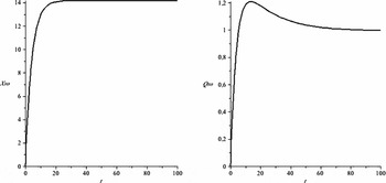
Figure 1 illustrates the accumulation patterns of the collective and individual stocks for a set of parameters such that both initial stocks are below their steady-state levels (see appendix A-3). The groundwater stock is indeed monotonously increasing, while the salt path first follows an increasing trend then decreases to approach the steady state. The first phase corresponds to the highly increasing part of the groundwater path; when it stabilizes, the high level of Q induces a higher rootzone salt decay rate so that the stock approaches its steady-state level from above.
Groundwater and rootzone salt socially optimal accumulation paths.

The remainder of this paper is dedicated to the design of corrective schemes to align individual decisions to the socially optimal ones.Footnote 5 Proposition 4 establishes the existence of taxation schemes allowing the regulator to induce individual agents to take decisions which lead to the socially optimal stationary levels of the stocks. This tax is coined efficient in this paper, as it allows optimal targets to be reached, but is not designed to induce optimal decisions during the transition to the steady state. Inducing the optimal accumulation of both stocks along the whole time horizon is the purpose of the tax whose existence is established in proposition 5.
4. Dynamic taxes in an open-loop framework
In this section, we assess the potential of various dynamic taxes to induce individual agents to take optimal decisions. We focus on two potential tax bases: the level of input and the state of the collective stock, and rule out the individual rootzone salt stocks. Within the framework of this model, this is motivated by the prohibitively high costs that the regulator would incur by monitoring the individual salt stocks. In a more general setting, this reflects the assumption that the regulator has better control and monitoring skills over the collective stock than over the set of individual ones. The following general water tax scheme is considered:

This formulation encompasses various dynamic taxes that have been analyzed in the literature previously: a time-independent emission tax (τ2 = τ3 = 0) (Ko et al., Reference Ko, Lapan and Sandler1992), a linear state-dependent ambient tax (τ1 = τ2 = 0) (Horan et al., Reference Horan, Shortle and Abler1998) and a linear Markov perfect emission tax (τ3 = 0) (Benchekroun and Long, Reference Benchekroun and Long1998).
The analyses are conducted under the assumption that the agents choose open-loop strategies: they base their decisions only on time, and on the initial stock level, and take the other agents' actions as given when determining their optimal trade-off between current and future irrigation decisions. This choice of strategy is motivated by the assumption that the agents can pre-commit to a set of decisions that they do not reassess over the course of the game. This illustrates a far-sighted environmental awareness by the agents (Dockner et al., Reference Dockner, Jorgensen, Long and Sorger2000) that applies more to water management at the catchment scale than to other settings.Footnote 6
Proposition 3 clarifies the impact of each type of parameter, attached either to an individual variable (τ1), a collective one (τ3) or both (τ2), on the steady-state level and the accumulation rate of the collective and individual stocks. Then in propositions 4 and 5, we show that the properties of efficiency and optimality of particular tax schemes, established in a single stock setting, extend to the framework with multiple correlated stocks analysed in this paper.
Proposition 3. When the tax scheme described in equation (7) is implemented, all the parameters of the tax impact on the steady-state levels of both stocks. However, only parameter τ2 impacts on the groundwater stock accumulation rate, thus indirectly on the accumulation of the rootzone salt stocks.
Proof. The first-order conditions and MHDS obtained in the case of taxed agents are presented in appendix B-1. The steady-state levels and eigenvalues are given by the following expressions:

with u τ∞(τ2) and M(τ2) given in appendix B-1.
From Proposition 3, the simple tax parameters, attached to the individual or the collective variables, have a clear effect on the steady-state stock levels. Indeed,  : a higher level of the tax decreases the steady-state accumulation level, not only of the collective stock that is directly targeted, but also of the individual stocks.
This proposition also highlights the special status of τ2, as it affects the accumulation rate ρτ1. A higher τ2 reduces the speed of accumulation of the collective stock (since  ). This indirectly affects the accumulation pattern of the individual stock:

Furthermore, as would be expected,  . However,
 cannot be signed analytically (see appendix B-1). This reflects the fact that τ2 impacts on the salt stock directly through its impact on the input level and indirectly through its impact on the groundwater stock level.
Next we provide the full derivation of the tax parameters in two settings. In the first step, the regulator is assumed to require the agents to comply with the optimal stock levels at the steady state. Considering multiple stocks does not alter the potential of single-parameter taxes to do so (see proposition 4). In the second step, we assume that the regulator adopts a more standard definition of efficiency, which is the requirement that the agents comply with the optimal stock levels along the whole time horizon. The type of tax that has been shown to bear this property in the case of a single stock is also optimal in the framework described in this paper (see Proposition 5).
Proposition 4. In a context where two pollution stocks interact as described by equations (1) and (2), a single-parameter tax induces the agents to reach the optimal steady-state level of the collective stock, as in the single stock setting, but also of the individual stocks, as an open-loop Nash equilibrium.
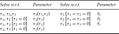
Proof. We solve the system {X ∞so = X ∞τ, Q ∞so = Q ∞τ} with respect to different combinations of the tax parameters, as described in table 1.
Efficient taxes (w.r.t.: with respect to)

The expressions of  and
 are provided in appendix B-2.
From table 1, any combination of the tax parameters defined in equation (7) allows the regulator to achieve the efficient solution, in the sense that has been defined in the paper. In particular, all single-parameter taxes are able to induce agents to reach the optimal stock levels at the steady state as an open-loop Nash equilibrium (OLNE). However, this does not guarantee that these levels are not reached earlier, or even exceeded, in the rootzone salts stock case. Indeed, the monotonicity of its accumulation path is not given (see appendix B-1).
The impact of the correlation term α on the tax parameters is as follows:

where  is given in appendix B-2. These expressions cannot be signed. However, the impact of the correlation term on the value of the taxes decreases as the social damage parameter increases. The higher the social damage associated to the collective stock, the smaller the relative impact of its indirect effect on the individual stocks.
Next we assess the potential of the tax scheme described in equation (7) to induce optimal decisions along the whole time horizon, rather than at the steady state only.
Proposition 5. In a context where two pollution stocks interact as described by equations (1) and (2), a tax τ* = u(τ*1 + τ*2X) induces the agents to achieve the optimal accumulation not only of the collective stock, as in the case of a single stock, but also of the individual stocks, as an OLNE.
Proof. We follow the methodology used by Benchekroun and Long (Reference Benchekroun and Long1998). We seek to have the agents, subject to the optimal tax scheme τ*(τ1, τ2, τ3), use the optimal reaction function uso(X) obtained in the socially optimal programme. Consider the following conditions derived from the programme of a taxed agent:


We extract an expression of λ from equation (8), derive it with respect to time and equate it to equation (9) to get:

In equation (10), we set  and
 . Finally, we replace u by uso(X) (hence
 by
 )Footnote 7 to get a first-order equation in X which has to equate zero for all values of X:

Refer to appendix B-3 for the expressions of R(τ2) and S(τ1, τ2, τ3). The optimal tax, obtained by solving {R(τ2) = 0, S(τ1, τ2, τ3) = 0} can take two forms,Footnote 8 either τ* = u(τ*1 + τ*2X) or τ* = X(τ*3 + τ*2u), with


According to proposition 5, the regulator can induce open-loop agents to achieve the optimal management of a collective stock and of a set of correlated individual stocks, by implementing a linear Markov perfect taxation scheme based on the collective stock and the individual levels of input. Inclusion of the individual stocks in the tax scheme is not necessary. This result is driven by the features of the correlation analysed in the paper: the collective stock has a linear impact on the individual ones. Furthermore, the social and individual valuations of the salt-related damage are equal: if the agents are induced to manage the groundwater stock optimally then they do not need further incentive relating to the salt stocks.
Proposition 5 also states that two configurations of the mixed corrective scheme lead to optimal irrigation decisions: a stock-dependent input tax and an ambient tax whose rate evolves with the individual input levels. The former expression of the corrective scheme applies more easily to the irrigation-induced salinity context, as water taxes are already implemented. Consequently, the following remarks are formulated for an optimal tax defined as τ* = u(τ*1 + τ*2X).
Remark 1. The optimal tax rate is composed of a term positively related to the collective stock level and of a constant whose sign cannot be determined analytically.
Refer to appendix B-4 for the demonstration that τ*2 > 0: the tax rate unambiguously increases with the collective stock, as for a unique stock (Benchekroun and Long, Reference Benchekroun and Long1998; Legras and Lifran, Reference Legras and Lifran2006). This is not surprising since inducing the agents to correctly internalize their impact on the current and future states of the stocks, the tax should send them the message that the more they contribute to the stocks now, the higher their tax liability will be in the future. The sign of τ*1 is more difficult to grasp. The first line of the right-hand side of equation (12) contains positive terms, the second line groups the negative ones. It can be noted that τ*1 is positively related to τ*2. Benchekroun and Long (Reference Benchekroun and Long1998) show that the polluting emissions of oligopolistic producers may be subsidized at the beginning of the time horizon in order to counterbalance the market power effect that arises in oligopolistic settings. In the case of groundwater management, no such strategic incentive was found (Legras and Lifran, Reference Legras and Lifran2006). However, numerical simulations conducted with the set of parameters depicted in appendix A-3 put in perspective that negative values of τ*1 are compatible with low values of β and high values of k 3; in other words, the rootzone salt stocks are highly detrimental, either because they accumulate fast or because the damage term is high. Subsidizing irrigation, in this case, increases the decay process of the rootzone stock by increasing the stock at the beginning of the time horizon.
Remark 2. The correlation term α only affects the constant term of the optimal tax.
It can easily be noted that  since
 . The sign of
 is ambiguous (appendix B-4). However, it is positive for the set of parameters used in our numerical simulations: the tax increases with the indirect impact of groundwater. As the marginal damage due to the rootzone salt is constant over time, it is accommodated by the constant part of the tax rate.
5. Conclusion
This paper examines the design of optimal water taxes to induce irrigators to take socially optimal decisions in a context where irrigation decisions contribute to the accumulation of individual stocks of rootzone salt and of a collective stock of groundwater. A key feature of this context is the fact that the collective stock has a direct impact on the individual ones. In this regard, it constitutes a special case of correlated stock externalities.
The main result of this paper is that optimal taxation schemes, to manage irrigation-induced salinity, need not be based on both types of stocks. Indeed, we show that individual agents take optimal decisions when they are subject to a linear Markov perfect tax, a water input tax whose rate depends on the state of the collective stock. Such a tax has been shown to be able to induce the optimal management of a groundwater stock by a group of agents. Due to the type of correlation described in this paper – a collective stock that affects a set of individual stocks in a linear fashion – the same type of tax scheme can be applied to induce the optimal management of both types of stocks. We also show that if the regulator's objective is to reach the optimal stock level at the steady state, she can rely on even simpler taxes, based on only one variable, the water input or the collective stock, as when there is only one stock to manage.
We restricted the analysis to a particular informational setting, which leaves strategic interaction issues aside. An extension to the case where agents choose feedback, rather than open-loop, strategies would introduce the strategic management of groundwater. In the single stock context, the feedback Nash equilibrium is characterized by higher stock levels than the OLNE. The most common assumption regarding feedback strategies in an accumulation problem is that each agent thinks that the others will react to an increase in the collective stock level by reducing their water input; consequently he's induced to increase his irrigation level to benefit from the others' reactions. In the present context, as the individual stocks are independent and cause damage to each irrigator, the strategic effect should be less important. Consequently, we expect the optimal feedback tax to be of the same form as in the single stock case, and to compare to the open-loop tax in the same manner (a higher tax rate to reduce strategic incentives).
The interactions between the stocks which are peculiar to the situation considered here enable us to capture the main features of irrigation-induced salinity. Alternative configurations would better describe other contexts; in the case of climate change, regional stocks of sulphur have a cooling effect on the global stock of carbon: the correlation is negative and directed from the individual stocks to the collective one. Extending the analysis of policy design to other cases of multiple, correlated pollutants is important as examples of such settings count among the most stringent current environmental issues.
Appendix A
A-1. Accumulation paths in the socially optimal programme. First note that

The eigenvalues and associated eigenvectors in the regulator's programme are

As ρ1μ = ρ2μ = ρ2X = ρ2λ = 0, the state and co-state accumulation paths are given by the following expressions, where the so subscripts have been dropped for the sake of readability:


Constants c 1 and c 2 solve the system of equations (14)–(15) for all t, in particular, t = 0:

A-2. Monotonicity properties of Qso(t). Qso(t) is non-monotonous if there is a non-nul time t at which its time-derivative changes sign (the so subscripts have been dropped):

A-3. Value of the parameters used in the numerical illustrations. n = 10, k 0 = 0.05, k 1 = 1.95, k 2 = 0.8, k 3 = 0.01, k 4 = 0.0005, k 5 = 0.01, δ = 0.02, α = 0.05, γ = 0.01, p = 1, β = 0.05, a = 0.6, b = 0.6, r = 0.04, Q 0 = X 0 = 0.
A-4. Programme of an individual agent. An agent using open-loop strategies has the following programme, where ū denotes the other agents' (exogenous) input choice:

The MHDS associated to this programme is as follows:

The accumulation paths are of similar form as in the socially optimal case, with

Appendix B
B-1. Programme of a taxed agent. An agent subject to the tax scheme described in equation (7) has the following programme, where ū denotes the other agents' (exogenous) input choice:

Rearranging the necessary conditions leads to

Then the Jacobian and the constant matrices are

The steady-state values are

The eigenvalues and eigenvectors are

The individual and collective stocks' accumulation paths are

Considering the following:

it is difficult to sign . Indeed, all expressions are negative except for  .
B-2. Parameters of the efficient taxes. The efficient taxes are given by  and
 , with

B-3. Value of R(τ2) and S(τ1, τ2, τ3).

B-4. Proof of Remark 1. From equation (11), we have

The denominator of τ*2 is positive as n > 1>a and ρso1 + δ + γ < 0. Then, we consider the following:

Noting R(a) = ρ*1−ρso1, we have:  and R(1) > 0. Hence the positivity of τ*2 is ensured. Furthermore, as
 : the value and sign of the correlation term has no direct impact on this parameter.
The sign of τ*3, hence of τ*1, is not clear. Remember that

The impact of α on τ*3 is not clear either:

 .
![$u_{\infty}^{m}=\frac{1}{pk_{2}}[pk_{1}+a\lambda _{\infty}^{m}+b\mu _{\infty}^{m}] (m\in \lbrack ol,so]), \mu _{\infty}^{so}=\mu _{\infty}^{ol}$](https://static.cambridge.org/binary/version/id/urn:cambridge.org:id:binary:20160920233657251-0920:S1355770X10000021:S1355770X10000021_inline20.gif?pub-status=live) and λol∞ > λso∞, it is straightforward to show that, with α > 0, Xso ∞ < Xol ∞ and Qso ∞ < Qol ∞. This motivates the need for a corrective instrument to align individual decisions to the social optimum.
 , since λso(t) = ρ1λXso(t) − ρ1λXso ∞ + λso∞.
 .