


%20--%3e%3c!DOCTYPE%20svg%20PUBLIC%20'-//W3C//DTD%20SVG%201.0//EN'%20'http://www.w3.org/TR/2001/REC-SVG-20010904/DTD/svg10.dtd'%3e%3csvg%20version='1.0'%20id='Layer_1'%20xmlns='http://www.w3.org/2000/svg'%20xmlns:xlink='http://www.w3.org/1999/xlink'%20x='0px'%20y='0px'%20width='64px'%20height='64px'%20viewBox='5.5%20-3.5%2064%2064'%20enable-background='new%205.5%20-3.5%2064%2064'%20xml:space='preserve'%3e%3cg%3e%3ccircle%20fill='%23FFFFFF'%20fill-opacity='0'%20cx='37.785'%20cy='28.501'%20r='28.836'/%3e%3cpath%20fill='%23595959'%20d='M37.441-3.5c8.951,0,16.572,3.125,22.857,9.372c3.008,3.009,5.295,6.448,6.857,10.314%20c1.561,3.867,2.344,7.971,2.344,12.314c0,4.381-0.773,8.486-2.314,12.313c-1.543,3.828-3.82,7.21-6.828,10.143%20c-3.123,3.085-6.666,5.448-10.629,7.086c-3.961,1.638-8.057,2.457-12.285,2.457s-8.276-0.808-12.143-2.429%20c-3.866-1.618-7.333-3.961-10.4-7.027c-3.067-3.066-5.4-6.524-7-10.372S5.5,32.767,5.5,28.5c0-4.229,0.809-8.295,2.428-12.2%20c1.619-3.905,3.972-7.4,7.057-10.486C21.08-0.394,28.565-3.5,37.441-3.5z%20M37.557,2.272c-7.314,0-13.467,2.553-18.458,7.657%20c-2.515,2.553-4.448,5.419-5.8,8.6c-1.354,3.181-2.029,6.505-2.029,9.972c0,3.429,0.675,6.734,2.029,9.913%20c1.353,3.183,3.285,6.021,5.8,8.516c2.514,2.496,5.351,4.399,8.515,5.715c3.161,1.314,6.476,1.971,9.943,1.971%20c3.428,0,6.75-0.665,9.973-1.999c3.219-1.335,6.121-3.257,8.713-5.771c4.99-4.876,7.484-10.99,7.484-18.344%20c0-3.543-0.648-6.895-1.943-10.057c-1.293-3.162-3.18-5.98-5.654-8.458C50.984,4.844,44.795,2.272,37.557,2.272z%20M37.156,23.187%20l-4.287,2.229c-0.458-0.951-1.019-1.619-1.685-2c-0.667-0.38-1.286-0.571-1.858-0.571c-2.856,0-4.286,1.885-4.286,5.657%20c0,1.714,0.362,3.084,1.085,4.113c0.724,1.029,1.791,1.544,3.201,1.544c1.867,0,3.181-0.915,3.944-2.743l3.942,2%20c-0.838,1.563-2,2.791-3.486,3.686c-1.484,0.896-3.123,1.343-4.914,1.343c-2.857,0-5.163-0.875-6.915-2.629%20c-1.752-1.752-2.628-4.19-2.628-7.313c0-3.048,0.886-5.466,2.657-7.257c1.771-1.79,4.009-2.686,6.715-2.686%20C32.604,18.558,35.441,20.101,37.156,23.187z%20M55.613,23.187l-4.229,2.229c-0.457-0.951-1.02-1.619-1.686-2%20c-0.668-0.38-1.307-0.571-1.914-0.571c-2.857,0-4.287,1.885-4.287,5.657c0,1.714,0.363,3.084,1.086,4.113%20c0.723,1.029,1.789,1.544,3.201,1.544c1.865,0,3.18-0.915,3.941-2.743l4,2c-0.875,1.563-2.057,2.791-3.541,3.686%20c-1.486,0.896-3.105,1.343-4.857,1.343c-2.896,0-5.209-0.875-6.941-2.629c-1.736-1.752-2.602-4.19-2.602-7.313%20c0-3.048,0.885-5.466,2.658-7.257c1.77-1.79,4.008-2.686,6.713-2.686C51.117,18.558,53.938,20.101,55.613,23.187z'/%3e%3c/g%3e%3c/svg%3e)
%20--%3e%3c!DOCTYPE%20svg%20PUBLIC%20'-//W3C//DTD%20SVG%201.0//EN'%20'http://www.w3.org/TR/2001/REC-SVG-20010904/DTD/svg10.dtd'%3e%3csvg%20version='1.0'%20id='Layer_1'%20xmlns='http://www.w3.org/2000/svg'%20xmlns:xlink='http://www.w3.org/1999/xlink'%20x='0px'%20y='0px'%20width='64px'%20height='64px'%20viewBox='5.5%20-3.5%2064%2064'%20enable-background='new%205.5%20-3.5%2064%2064'%20xml:space='preserve'%3e%3cg%3e%3ccircle%20fill='%23FFFFFF'%20fill-opacity='0'%20cx='37.637'%20cy='28.806'%20r='28.276'/%3e%3cg%3e%3cpath%20fill='%23595959'%20d='M37.443-3.5c8.988,0,16.57,3.085,22.742,9.257C66.393,11.967,69.5,19.548,69.5,28.5c0,8.991-3.049,16.476-9.145,22.456%20C53.879,57.319,46.242,60.5,37.443,60.5c-8.649,0-16.153-3.144-22.514-9.43C8.644,44.784,5.5,37.262,5.5,28.5%20c0-8.761,3.144-16.342,9.429-22.742C21.101-0.415,28.604-3.5,37.443-3.5z%20M37.557,2.272c-7.276,0-13.428,2.553-18.457,7.657%20c-5.22,5.334-7.829,11.525-7.829,18.572c0,7.086,2.59,13.22,7.77,18.398c5.181,5.182,11.352,7.771,18.514,7.771%20c7.123,0,13.334-2.607,18.629-7.828c5.029-4.838,7.543-10.952,7.543-18.343c0-7.276-2.553-13.465-7.656-18.571%20C50.967,4.824,44.795,2.272,37.557,2.272z%20M46.129,20.557v13.085h-3.656v15.542h-9.944V33.643h-3.656V20.557%20c0-0.572,0.2-1.057,0.599-1.457c0.401-0.399,0.887-0.6,1.457-0.6h13.144c0.533,0,1.01,0.2,1.428,0.6%20C45.918,19.5,46.129,19.986,46.129,20.557z%20M33.042,12.329c0-3.008,1.485-4.514,4.458-4.514s4.457,1.504,4.457,4.514%20c0,2.971-1.486,4.457-4.457,4.457S33.042,15.3,33.042,12.329z'/%3e%3c/g%3e%3c/g%3e%3c/svg%3e)
1. Introduction
Baran et al. (Reference Baran2023, Reference Baran, Charpinet, Østensen, Reed, Van Grootel, Lyu, Telting and Németh2024) searched for short period hot subdwarf pulsators observed by the Transiting Exoplanet Survey Satellite (TESS). Baran et al. (Reference Baran, Charpinet, Østensen, Reed, Van Grootel, Lyu, Telting and Németh2024) also reported conclusions on correlations between asteroseismic and atmospheric parameters, as well as the instability strip of hot subdwarfs. They reported 93 pulsators, i.e. 67 subdwarf B (sdB) stars, 23 subdwarf OB (sdOB) stars, two subdwarf O (sdO) stars, and, significantly, one He-sdOB star, which is the first of this kind to show short-period pulsations.
We continued the effort originally started by Baran et al. (Reference Baran2023), with the ultimate goal to provide a census of the pressure-mode (p-mode) dominated hot-subdwarf stars surveyed by the TESS mission, along with an ensemble analysis on the presence of p-mode pulsators among hot subdwarfs. In this report we present results of our analysis of p-mode hot subdwarf pulsators found in TESS data collected over Sectors 61 and 97, i.e. Years 5–7 of TESS operations + Sector 97.
2. Classification spectra
To verify or establish the spectral classification of unclassified objects, for which we do not possess reliable spectroscopic data, we obtained new spectra using the ALFOSC spectrograph on the 2.56 m Nordic Optical Telescope (NOT). We utilised grism #18 that covers the Balmer series from H
 $_\beta$
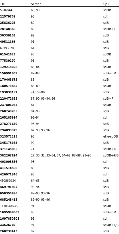
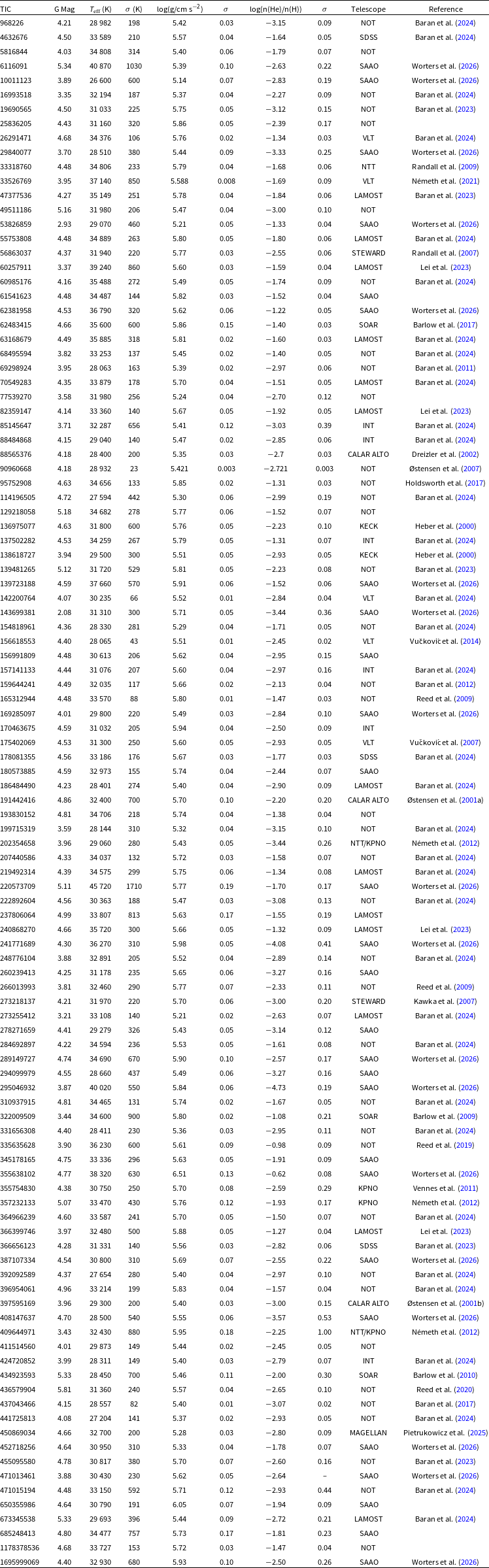
blueward, spanning 3 450–5 350 Å. We made use of a 0.5-arcsec slit resulting in 0.93 Å/pixel dispersion. The values we derived are listed in Section 4. Another set of spectrograms for the target stars was obtained with the 1.9 m telescope at the Sutherland site of the South African Astronomical Observatory (SAAO) using the Cassegrain spectrograph with grating 6 and a 1.0-arcsec slit to give a spectral range of about 3 500–6 000 Å, at around 1.35 Å/pixel. Spectral types (SpT), either from the literature or from new spectroscopy that we acquired for this work, are listed in Table 1. We followed the classification convention adopted by Baran et al. (Reference Baran2023). Spectroscopic parameters are listed in Table 2. To determine spectroscopic parameters,
 $T_\textrm{eff}$
,
 $\log\,g$
, and
 $\log$
(n(He)/n(H)), for which we have obtained new spectra, we fitted the LTE model atmospheres (Heber et al. Reference Heber, Reid and Werner2000; Edelmann et al. Reference Edelmann, Heber, Hagen, Lemke, Dreizler, Napiwotzki and Engels2003) used in many previous works including Baran et al. (Reference Baran, Charpinet, Østensen, Reed, Van Grootel, Lyu, Telting and Németh2024). This minimised the systematic effects when comparing atmospheric parameters. For all the spectra we fitted the hydrogen lines, H
 $_{\beta}$
through H
 $_{12}$
, as well as the HeI lines at 4 026 and 4 472 Å, and the HeII line at 4 686 Å. The continuum was fitted outside the wings of each line, following the classic method described in Heber et al. (Reference Heber, Reid and Werner1999). As long as the highest order of Balmer lines visible are included and there are no spectroscopic artifacts in this region, the continuum placement should not affect the surface gravity.
The list of pulsating hot subdwarfs found in the TESS data. Only sectors with the USC data collected are listed. New pulsators, found only in the TESS data, are marked with bold font. The first p-mode dominated heavy-metal hot subdwarf and another hot subdwarf pulsator detected in Sector 97 of TESS are listed at the bottom and are separated from the targets observed during Years 5–7.

Table 1. Long description
The table lists pulsating hot subdwarfs identified in the TESS data, detailing their TIC identifiers, sectors, and spectral types. The table has three columns: TIC, Sector, and SpT. The TIC column lists unique identifiers for each object. The Sector column lists the sectors in which the data were collected, with some sectors containing multiple values. The SpT column lists the spectral types of the objects. Notable entries include new pulsators found only in the TESS data, marked with bold font, and specific objects listed at the bottom of the table. The table includes 40 rows of data.
3. TESS photometry
We follow the approach of Baran et al. (Reference Baran2023, Reference Baran, Charpinet, Østensen, Reed, Van Grootel, Lyu, Telting and Németh2024). Data were downloaded from the Barbara A. Mikulski Archive for Space Telescopes (MAST).Footnote
a
Unlike previous reports, here we used only the USC data (ultra-short cadence with a total of 20 s integration, including any overheads), which practically guarantee that the entire p-mode frequency range is sampled. We used PDCSAP_FLUX and first we clipped fluxes at 4.5
 $\unicode{x03C3}$
to remove outliers, if necessary. Next, we de-trended long-term variations with spline fitting, and scaled the flux making the amplitude of the flux variation to be given as parts-per-thousand (ppt). The ppt does not apply to six stars, i.e. TIC 10011123, TIC 289149727, TIC 295046932, TIC 450869034, TIC 1178378536 and TIC 1695999069. We suspect that their fluxes are underestimated by an overestimated background level or incorrect crowding correction, which caused the average flux level to be unrealistic. Therefore, the amplitudes of their flux variations are not accurate.
4. Fourier analysis
We used a standard prewhitening technique. More details can be found in Baran et al. (Reference Baran2023). Based on results presented by Baran & Koen (Reference Baran and Koen2021), we adopted a detection threshold at a signal-to-noise (S/N) of 5 times the median noise level, regardless of the data coverage. Significant signal in the p-mode region was found in 36 hot subdwarfs, including 33 stars not known to pulsate prior to the TESS mission. A list of all 36 p-mode hot subdwarf pulsators is given in Table 1. Below, we describe each target, including relevant pre-TESS history. To be consistent with the previous studies, the layout of each paragraph is adopted from Baran et al. (Reference Baran2023, Reference Baran, Charpinet, Østensen, Reed, Van Grootel, Lyu, Telting and Németh2024). Amplitude spectra and the list of frequencies detected from the TESS light curves are also included. In the case of the TESS discoveries, we only refer to those papers that supplement our results, and hence advance the knowledge of a specific star.
The Nyquist frequency of USC data, 25 000
 $\unicode{x03BC}$
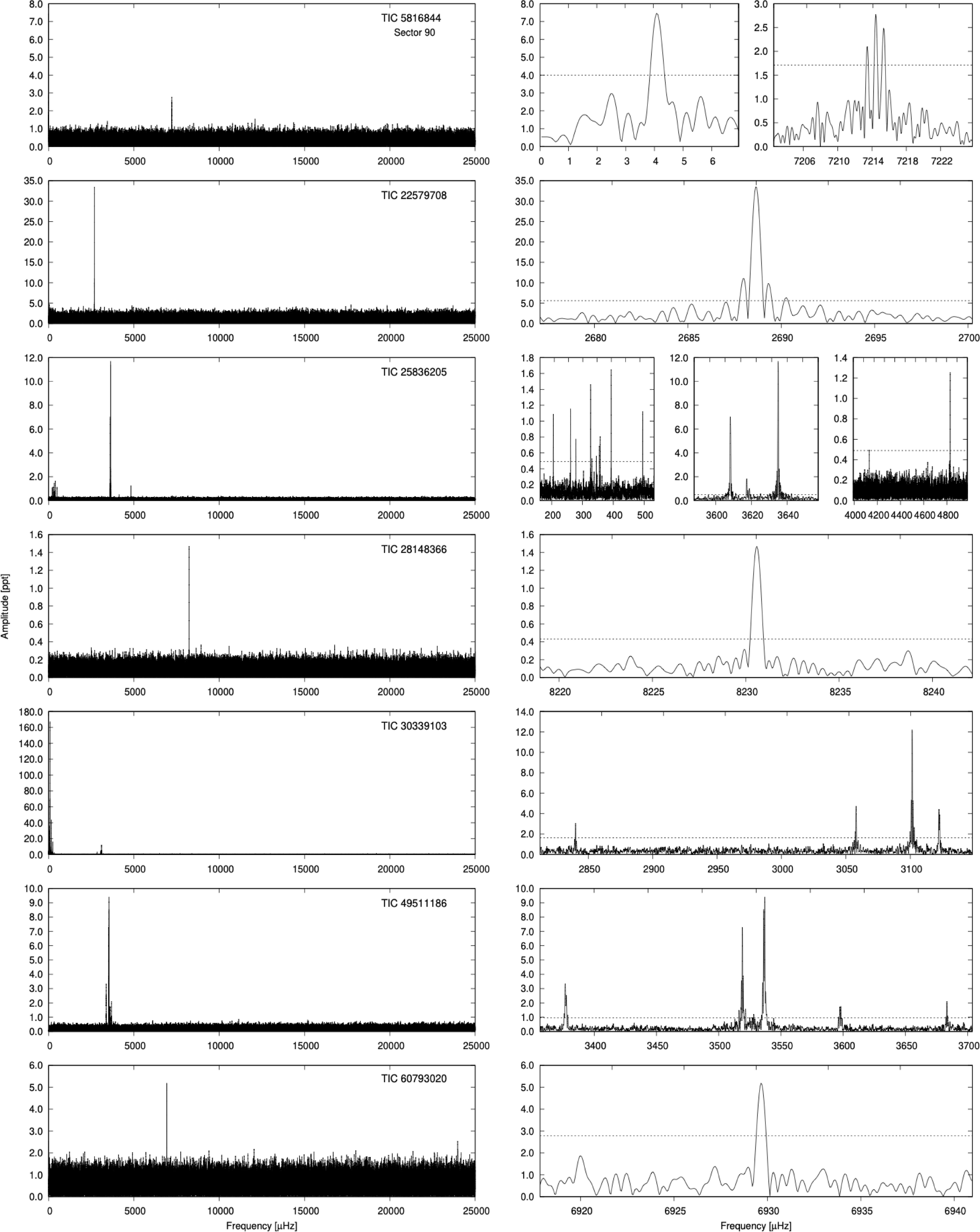
Hz, is well beyond the expected pulsation frequencies of virtually all known hot subdwarfs, so the USC mode provides us with a unique frequency identification. Therefore, we decided not to include any SC data in this paper, even those taken in sectors without available USC data. Table 1 provides detailed sector information. We show the amplitude spectra of USC-observed sdBV stars in Figures 1 through 5 and provide the seismic properties in Table 3.
Spectroscopic estimates of pulsating hot subdwarfs reported here, for which we derived acceptable spectroscopic fits. Blank reference means ‘this work’. The stars already listed in Table 3 of Baran et al. (Reference Baran, Charpinet, Østensen, Reed, Van Grootel, Lyu, Telting and Németh2024) are also included to account for more recent measurements and to complement the whole sample with Gaia absolute magnitudes.

Table 2. Long description
Panel A: Line graph displaying spectroscopic estimates of pulsating hot subdwarfs. The x-axis represents different stars, and the y-axis represents spectroscopic estimates in unspecified units. Panel B: Line graph showing Gaia absolute magnitudes for the same stars. The x-axis represents different stars, and the y-axis represents absolute magnitudes in unspecified units. Panel C: Table listing spectral types and other parameters for the stars, including effective temperature, surface gravity, and helium to hydrogen ratio.
TIC 5816844 (Gaia DR3 3517127900988821504) was not identified as a pulsator prior to the TESS mission. Kilkenny et al. (Reference Kilkenny, O’Donoghue, Koen, Stobie and Chen1997b) classified the star as sdO. From our fit to a spectrum taken with the NOT, we derived
 $T_\textrm{eff}$
= 34 808(314) K,
 $\log$
(g/
 $\mbox{cm}\,\mbox{s}^{-2}$
) = 5.40(6) and
 $\log$
(n(He)/n(H)) =
 $-1.79(7)$
, which indicates an sdOB type. TESS observed the star during Sectors 63 and 90. We detected three frequencies in Sector 63 and four frequencies in Sector 90 – all in the p-mode region. We show the amplitude spectrum calculated from Sector 63 data in Figure 1, and we list the prewhitened frequencies in Table 3. The dominant amplitude frequency is usually interpreted as a binary frequency. In this case, however, the amplitude decreased by a factor of nearly three over two years, suggesting that the binary interpretation may not survive. Three frequencies, detected in Sector 90, make a slightly asymmetric triplet. Assuming they are rotationally split modes, the average rotation period is 12.4(0.2) days.
TIC 22579708 (Gaia DR3 5954753799767211904) was not identified as a pulsator prior to the TESS mission. Based on the Gaia colour index
 $B_{p}-R_{p}=-0.21$
and absolute magnitude
 $G_\textrm{ Mag}$
= 4.55, the star is considered a hot subdwarf. TESS observed the star during Sector 93. We detected only one frequency in the p-mode region. We show the amplitude spectrum in Figure 1, and we list the prewhitened frequency in Table 3.
TIC 25836205 (Gaia DR3 5439887654492064256) was not identified as a pulsator prior to the TESS mission. Sahoo et al. (Reference Sahoo, Baran, Sanjayan and Ostrowski2020) found it to be a pulsator candidate, while Sahoo et al. (Reference Sahoo, Baran, Worters, Németh and Kilkenny2023) classified the star as sdB. Worters et al. (Reference Worters, Kilkenny, Nemeth, Baran and Østensen2026) reported
 $T_\textrm{eff}$
,
 $\log$
(g/
 $\mbox{cm}\,\mbox{s}^{-2}$
) and
 $\log$
(n(He)/n(H)) to be 31,160(320) K, 5.86(5) and
 $-2.39(17)$
, respectively. TESS observed the star during Sector 89. We detected 16 frequencies, 10 in the gravity mode (g-mode) region, and six in the p-mode region. The star is a hybrid pulsator. We show the amplitude spectrum in Figure 1, and we list the prewhitened frequencies in Table 3. Figure 7 in Sahoo et al. (Reference Sahoo, Baran, Worters, Németh and Kilkenny2023) shows most of the frequencies we detected in Sector 89. The low Nyquist frequency of the data analysed by Sahoo et al. (Reference Sahoo, Baran, Worters, Németh and Kilkenny2023) resulted in no p-mode detection.
TIC 28148366 (Gaia DR3 1880197529545177856) was not identified as a pulsator prior to the TESS mission. Based on the absorption features in a spectrum collected with the William Herschel Telescope (WHT) in 2010, we classified this star as sdOB+F. TESS observed the star during Sector 83. We detected only one frequency in the p-mode region. We show the amplitude spectrum in Figure 1, and we list the prewhitened frequency in Table 3.
TIC 30339103 (Gaia DR3 6760700912479537536) was not identified as a pulsator prior to the TESS mission. Sahoo et al. (Reference Sahoo, Baran, Sanjayan and Ostrowski2020) detected one frequency at around 80
 $\unicode{x03BC}$
Hz, too low to be considered a hot subdwarf pulsator. Subsequently, Sahoo et al. (Reference Sahoo, Baran, Worters, Németh and Kilkenny2023) reported that the signal was from a contaminator, which is Gaia DR2 6760700912479534336. Based on the absorption features in a spectrum, collected with the NTT telescope, we classified this star as sdB. TESS observed the star during Sector 92. We detected five frequencies in the p-mode region. We also detected a low frequency along with its six harmonics, intrinsic to Gaia DR2 6760700912479534336. We detected the fundamental frequency at 40.14315(17)
 $\unicode{x03BC}$
Hz, which translates to an orbital period of 0.2883200(12) days. Comparing frequencies we find that Sahoo et al. (Reference Sahoo, Baran, Sanjayan and Ostrowski2020) detected only the first harmonic, which is the highest amplitude signal in the data. We show the amplitude spectrum limited to the p-modes of our target in Figure 1, and we list the prewhitened p-mode frequencies in Table 3.
TIC 49511186 (Gaia DR3 6245429322278170880) was not identified as a pulsator prior to the TESS mission. From our fit to a spectrum taken with the NOT, we derived
 $T_\textrm{eff}$
= 31 980(206) K,
 $\log$
(g/
 $\mbox{cm}\,\mbox{s}^{-2}$
) = 5.47(0.04) and
 $\log$
(n(He)/n(H)) =
 $-3.00(10)$
, which indicates an sdB type. TESS observed the star during Sector 91. We detected nine frequencies, all in the p-mode region. We show the amplitude spectrum in Figure 1, and we list the prewhitened frequencies in Table 3.
Amplitude spectra of targets observed in the USC mode. If sector is not specified, we included all USC data. Left panels: Frequency range up to the Nyquist frequency. Right panels: Close-ups of the detected frequencies. In case of TIC 5816844 only local frequency range was used to calculate the threshold dashed line for the
 $\Omega$
frequency.

List of frequencies we detected in the targets observed in the USC. If sector is not specified, we included all USC data.

Table 3. Long description
The table presents a detailed list of frequencies detected in targets observed in the USC. It includes columns for Did, N 1, Bucket, Sector, T mag, log10Q, and Telescope. The table has 100 rows and 8 columns. Column headers are Did, N 1, Bucket, Sector, T mag, log10Q, and Telescope. Row labels are not present. The table provides specific values for each row under these headers. For example, Row 1: Did, 9; N 1, 28.221196; Bucket, bucket_2; Sector, 1; T mag, 10.35; log10Q, -3.05; Telescope, TESS. Row 2: Did, 10; N 1, 28.221196; Bucket, bucket_2; Sector, 1; T mag, 10.35; log10Q, -3.05; Telescope, TESS. The table continues in this format, providing detailed frequency information for each target. Notable trends or outliers are not explicitly mentioned as the table focuses on presenting raw data.
TIC 60793020 (V361 Hya, Gaia DR3 6270542648891154304) is the prototype of pulsating hot subdwarfs (EC14026-2647). It was reported as an sdB pulsator by Kilkenny et al. (Reference Kilkenny, Koen, O’Donoghue and Stobie1997a). TESS observed the star during Sector 64 from which we detected only one frequency in the p-mode region. It is the same signal as reported in the discovery paper by Kilkenny et al. (Reference Kilkenny, Koen, O’Donoghue and Stobie1997a). We show the amplitude spectrum in Figure 1, and we list the prewhitened frequency in Table 3.
TIC 61541623 (Gaia DR3 5379010620540123904) was not identified as a pulsator prior to the TESS mission. From our fit to a spectrum taken with the 1.9 m telescope at SAAO, we derived
 $T_\textrm{eff}$
= 34 847(144) K,
 $\log$
(g/
 $\mbox{cm}\,\mbox{s}^{-2}$
) = 5.82(3) and
 $\log$
(n(He)/n(H)) =
 $-1.52(4)$
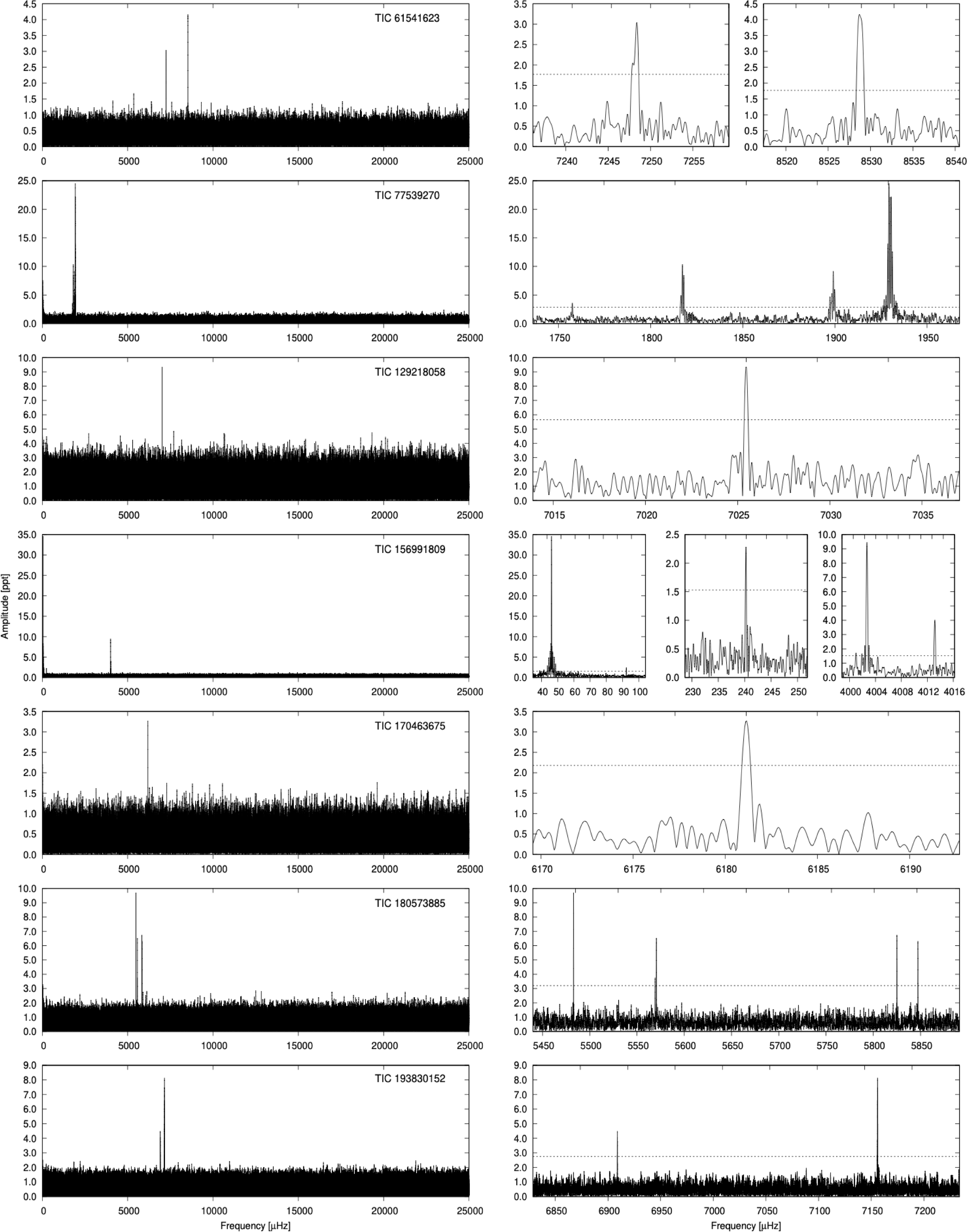
, which indicates an sdOB type. TESS observed the star during Sector 90. We detected four frequencies, all in the p-mode region. We show the amplitude spectrum in Figure 2, and we list the prewhitened frequencies in Table 3.
TIC 77539270 (Gaia DR3 6041128894929311872) was not identified as a pulsator prior to the TESS mission. From our fit to a spectrum taken with the NOT, we derived
 $T_\textrm{eff}=31\,980(256)$
K,
 $\log$
(g/
 $\mbox{cm}\,\mbox{s}^{-2}$
) = 5.24(4) and
 $\log$
(n(He)/n(H)) =
 $-2.70(12)$
, which indicates an sdB type. TESS observed the star during Sector 91. We detected seven frequencies, all in the p-mode region. The low-frequency sequence of harmonics is a contamination from CRTS J155634.6-290230, which is a known eclipsing binary system. We show the amplitude spectrum in Figure 2, and we list the prewhitened frequencies in Table 3.
TIC 129218058 (Gaia DR3 1932829364462415488) was not identified as a pulsator prior to the TESS mission. Mickaelian (Reference Mickaelian2008) classified the star as a hot subdwarf star. From our fit to a spectrum taken with the NOT, we derived
 $T_\textrm{eff}=34\,682(278)$
K,
 $\log$
(g/
 $\mbox{cm}\,\mbox{s}^{-2}$
) = 5.77(6) and
 $\log$
(n(He)/n(H)) =
 $-1.52(7)$
, which indicates an sdOB type. TESS observed the star during Sectors 83–84. We detected only one frequency in the p-mode region. We show the amplitude spectrum in Figure 2, and we list the prewhitened frequency in Table 3.
Amplitude spectra of targets observed in the USC mode. If sector is not specified, we included all USC data. Left panels: Frequency range up to the Nyquist frequency. Right panels: Close-ups of the detected frequencies.

Figure 2. Long description
The image contains multiple line graphs showing amplitude spectra of targets observed in the USC mode. Each target is represented by a pair of graphs: one showing the frequency range up to the Nyquist frequency and another providing a close-up of the detected frequencies. Panel A: The first pair of graphs for TIC 61541623 shows a broad frequency range up to 25000 microhertz on the left and a zoomed-in view of frequencies around 7240 to 7255 microhertz and 8520 to 8540 microhertz on the right. Panel B: The second pair of graphs for TIC 77539270 displays a similar broad frequency range up to 25000 microhertz on the left and a zoomed-in view of frequencies around 1750 to 1950 microhertz on the right. Panel C: The third pair of graphs for TIC 129218058 shows a broad frequency range up to 25000 microhertz on the left and a zoomed-in view of frequencies around 7015 to 7035 microhertz on the right. Panel D: The fourth pair of graphs for TIC 156991809 includes a broad frequency range up to 25000 microhertz on the left and zoomed-in views of frequencies around 40 to 100 microhertz, 230 to 250 microhertz, and 4000 to 4016 microhertz on the right. Panel E: The fifth pair of graphs for TIC 170463675 shows a broad frequency range up to 25000 microhertz on the left and a zoomed-in view of frequencies around 6170 to 6190 microhertz on the right. Panel F: The sixth pair of graphs for TIC 180573885 displays a broad frequency range up to 25000 microhertz on the left and a zoomed-in view of frequencies around 5450 to 5850 microhertz on the right. Panel G: The seventh pair of graphs for TIC 193830152 shows a broad frequency range up to 25000 microhertz on the left and a zoomed-in view of frequencies around 6850 to 7200 microhertz on the right. Each graph has amplitude in percent on the vertical axis and frequency in microhertz on the horizontal axis. The close-up graphs highlight specific frequency ranges where detected frequencies are observed, providing detailed views of the spectral characteristics of each target.
TIC 156991809 (Gaia DR3 5557300038753212544) was not identified as a pulsator prior to the TESS mission. From our fit to a spectrum taken with the 1.9 m telescope at SAAO, we derived
 $T_\textrm{eff}$
=
 $30\,613(206)$
K,
 $\log$
(g/
 $\mbox{cm}\,\mbox{s}^{-2}$
) = 5.62(4) and
 $\log$
(n(He)/n(H)) =
 $-2.95(15)$
, which indicates an sdB type. TESS observed the star during Sectors 87–88. We detected five frequencies. The dominant amplitude frequency and its first harmonic probably result from binary variability, with the secondary companion being a main sequence M star. One frequency was found in the g-mode region, while the remaining two were found in the p-mode region. The star is a hybrid pulsator. We show the amplitude spectrum in Figure 2, and we list the prewhitened frequency in Table 3.
TIC 170463675 (Gaia DR3 3063581068223451904) was not identified as a pulsator prior to the TESS mission. From our fit to a spectrum taken with the Isaac Newton Telescope (INT) in 2011, we derived
 $T_\textrm{eff}=31\,032(205)$
K,
 $\log$
(g/
 $\mbox{cm}\,\mbox{s}^{-2}$
) = 5.94(4) and
 $\log$
(n(He)/n(H)) =
 $-2.50(9)$
, which indicates an sdB type. TESS observed the star during Sector 88 and we detected only one frequency in the p-mode region. We show the amplitude spectrum in Figure 2, and we list the prewhitened frequency in Table 3.
TIC 180573885 (Gaia DR3 5530407633618087808) was not identified as a pulsator prior to the TESS mission. From our fit to a spectrum taken with the 1.9 m telescope at SAAO, we derived
 $T_\textrm{eff}=32\,973(155)$
K,
 $\log$
(g/
 $\mbox{cm}\,\mbox{s}^{-2}$
) = 5.74(4) and
 $\log$
(n(He)/n(H)) =
 $-2.44(7)$
, which indicates an sdOB type. TESS observed the star during Sectors 88–89. We detected five frequencies, all in the p-mode region. We show the amplitude spectrum in Figure 2, and we list the prewhitened frequencies in Table 3.
TIC 193830152 (Gaia DR3 1346490462254006656) was not identified as a pulsator prior to the TESS mission. Mickaelian (Reference Mickaelian2008) classified the star as sdB. From our fit to a spectrum taken with the NOT, we derived
 $T_\textrm{eff}=34\,706(218)$
K,
 $\log$
(g/
 $\mbox{cm}\,\mbox{s}^{-2}$
) = 5.74(4) and
 $\log$
(n(He)/n(H)) =
 $-1.38(4)$
, which indicates an sdB type. TESS observed the star during Sectors 74, 79–80 and we detected two frequencies, both in the p-mode region. We show the amplitude spectrum in Figure 2, and we list the prewhitened frequencies in Table 3.
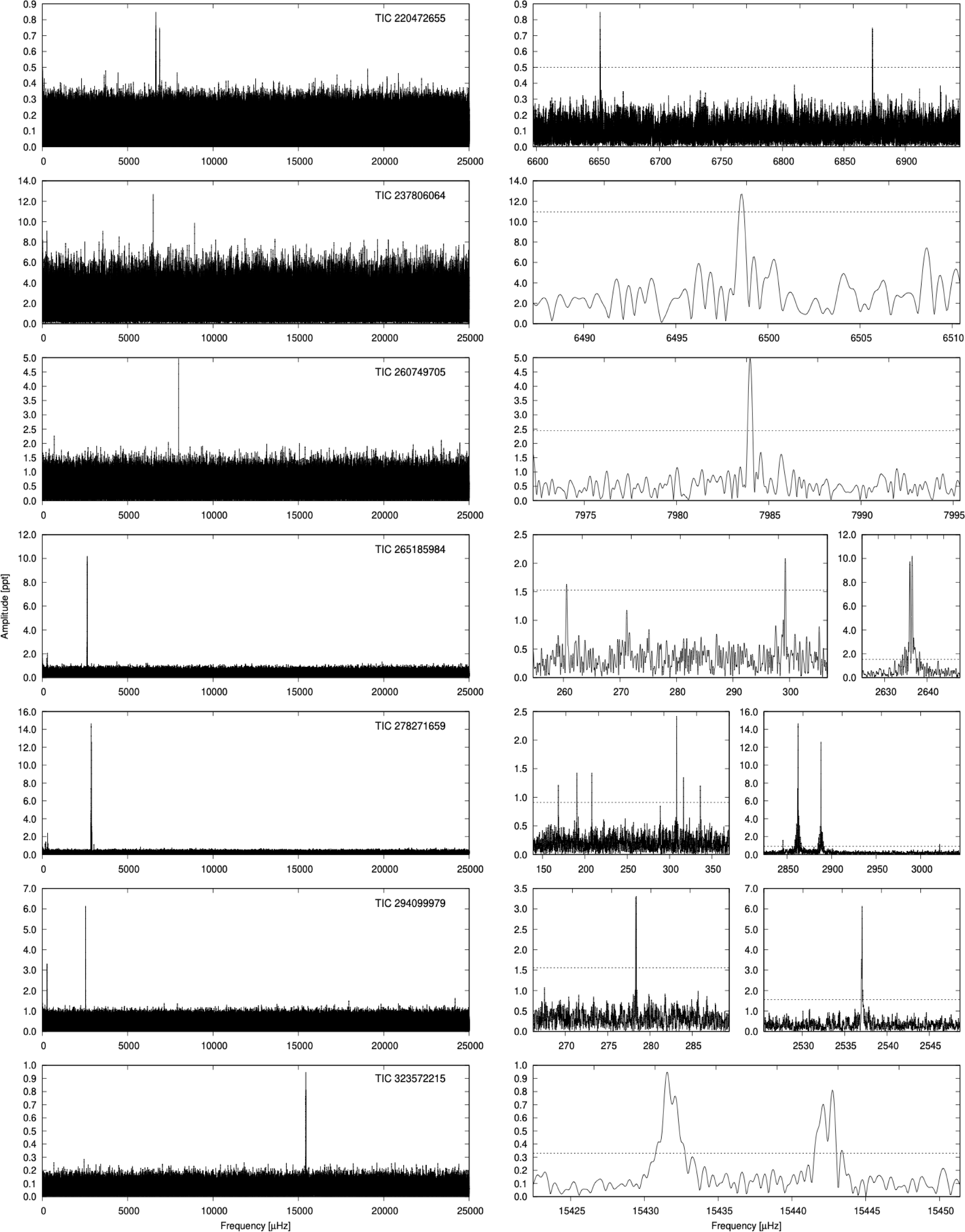
TIC 220472655 (Gaia DR3 4764744256126479104) was not identified as a pulsator prior to the TESS mission. O’Donoghue et al. (Reference O’Donoghue, Kilkenny, Koen, Hambly, MacGillivray and Stobie2013) classified the star as sdB+F. TESS observed the star during Sectors 87, 90, 93 – 94, 96. We detected three frequencies, all in the p-mode region. We show the amplitude spectrum in Figure 3, and we list the prewhitened frequencies in Table 3.
Amplitude spectra of targets observed in the USC mode. If sector is not specified, we included all USC data. Left panels: Frequency range up to the Nyquist frequency. Right panels: Close-ups of the detected frequencies.

TIC 237806064 (Gaia DR3 3129475762151272448) was not identified as a pulsator prior to the TESS mission. Luo et al. (Reference Luo, Németh, Wang, Wang and Han2021) derived
 $T_\textrm{eff}$
and
 $\log$
(g/
 $\mbox{cm}\,\mbox{s}^{-2}$
) to be 34 160(313) K and 5.71(6), respectively. From our fit to a spectrum taken with the LAMOST telescope, we derived
 $T_\textrm{eff}=33\,807(813)$
K,
 $\log$
(g/
 $\mbox{cm}\,\mbox{s}^{-2}$
) = 5.63(17) and
 $\log$
(n(He)/n(H))
 $=-1.55(19)$
, which indicates an sdOB type. The
 $T_\textrm{eff}$
and
 $\log$
(g/
 $\mbox{cm}\,\mbox{s}^{-2}$
) we derived are consistent with the values reported by Luo et al. (Reference Luo, Németh, Deng and Han2019). TESS observed the star during Sector 87 and we detected only one frequency in the p-mode region. We show the amplitude spectrum in Figure 3, and we list the prewhitened frequency in Table 3.
TIC 260749705 (Gaia DR3 6390633817137530752) was not identified as a pulsator prior to the TESS mission. Kilkenny et al. (Reference Kilkenny, O’Donoghue, Worters, Koen, Hambly and MacGillivray2015) classified the star as sdB. TESS observed the star during Sectors 94–95. We detected only one frequency in the p-mode region. We show the amplitude spectrum in Figure 3, and we list the prewhitened frequency in Table 3.
TIC 265185984 (Gaia DR3 6347311787693734784) was not identified as a pulsator prior to the TESS mission. Based on the Gaia colour index
 $B_{p}-R_{p}=-0.12$
and absolute magnitude
 $G_\textrm{ Mag}=4.61$
, the star is considered a hot subdwarf. TESS observed the star during Sectors 93–94. We detected five frequencies, two in the g-mode region and three in the p-mode region, which makes this star a hybrid pulsator. We show the amplitude spectrum in Figure 3, and we list the prewhitened frequency in Table 3. The p-modes are equally spaced in frequency. If we assume the frequency splitting of 0.540(11)
 $\unicode{x03BC}$
Hz is rotationally induced, this translates into a rotation period of 21.43(44) days.
TIC 278271659 (Gaia DR3 5194429968584799360) was not identified as a pulsator prior to the TESS mission. From our fit to a spectrum taken with the 1.9 m telescope at SAAO, we derived
 $T_\textrm{eff}=29\,279(326)$
K,
 $\log$
(g/
 $\mbox{cm}\,\mbox{s}^{-2}$
) = 5.43(5) and
 $\log$
(n(He)/n(H))
 $=-3.14(15)$
, which indicates an sdB type. TESS observed the star during Sectors 93–94. We detected 14 frequencies, both in the g- and p-mode regions, which makes this star a hybrid pulsator. We show the amplitude spectrum in Figure 3, and we list the prewhitened frequencies in Table 3. Frequencies around
 $f_9$
and
 $f_{12}$
could be triplets, although the splittings, if rotationally induced, are not symmetric. The average splitting in each triplet is around 0.47 and 0.56
 $\unicode{x03BC}$
Hz, which translates into a rotation period between 20 and 25 days.
TIC 294099979 (Gaia DR3 5485756878718056448) was not identified as a pulsator prior to the TESS mission. From our fit to a spectrum taken with the 1.9 m telescope at SAAO, we derived
 $T_\textrm{eff}=28\,660(437)$
K,
 $\log$
(g/
 $\mbox{cm}\,\mbox{s}^{-2}$
) = 5.49(6) and
 $\log$
(n(He)/n(H))
 $=-3.27(16)$
, which indicates an sdB type. TESS observed the star during Sectors 87–90, 93–96. We detected three frequencies, two in the g-mode region and one in the p-mode region. This star is a hybrid pulsator. We show the amplitude spectrum in Figure 3, and we list the prewhitened frequencies in Table 3.
TIC 323572215 (Gaia DR3 5196716471734490368) was not identified as a pulsator prior to the TESS mission. Based on the absorption features in a spectrum, collected with the 1.9 m telescope at SAAO, we classified this star as He-sdOB with a temperature above 40 000 K, a high surface gravity of around 6, and a He-abundance of 100x solar. In fact, according to the definition used by Baran et al. (Reference Baran2023), this star qualifies as a He-enhanced hot subdwarf. Sahoo et al. (Reference Sahoo, Baran, Worters, Németh and Kilkenny2023) found no pulsators in the He-enriched domain, therefore TIC 323572215 must be considered as the first detection of a pulsating He-enhanced hot subdwarf. TESS observed the star during Sector 93. We detected two signals at very high frequencies. The profiles of the peaks are very complex, indicative of unresolved frequencies, unstable amplitudes or unstable frequencies, similar to KIC 10139564 and KIC 2991276, which both show stochastic pulsations (Baran et al. Reference Baran2012; Østensen et al. Reference Østensen, Reed, Baran and Telting2014). We show the amplitude spectrum in Figure 3. Since prewhitening of such signals is hardly possible, in Table 3 we only list eyeball estimations of the signal.
TIC 345178165 (Gaia DR3 3460265248409925888) was not identified as a pulsator prior to the TESS mission. From our fit to a spectrum taken with the 1.9 m telescope at SAAO, we derived
 $T_\textrm{eff}=33\,336(296)$
K,
 $\log$
(g/
 $\mbox{cm}\,\mbox{s}^{-2}$
) = 5.63(5) and
 $\log$
(n(He)/n(H))
 $=-1.91(9)$
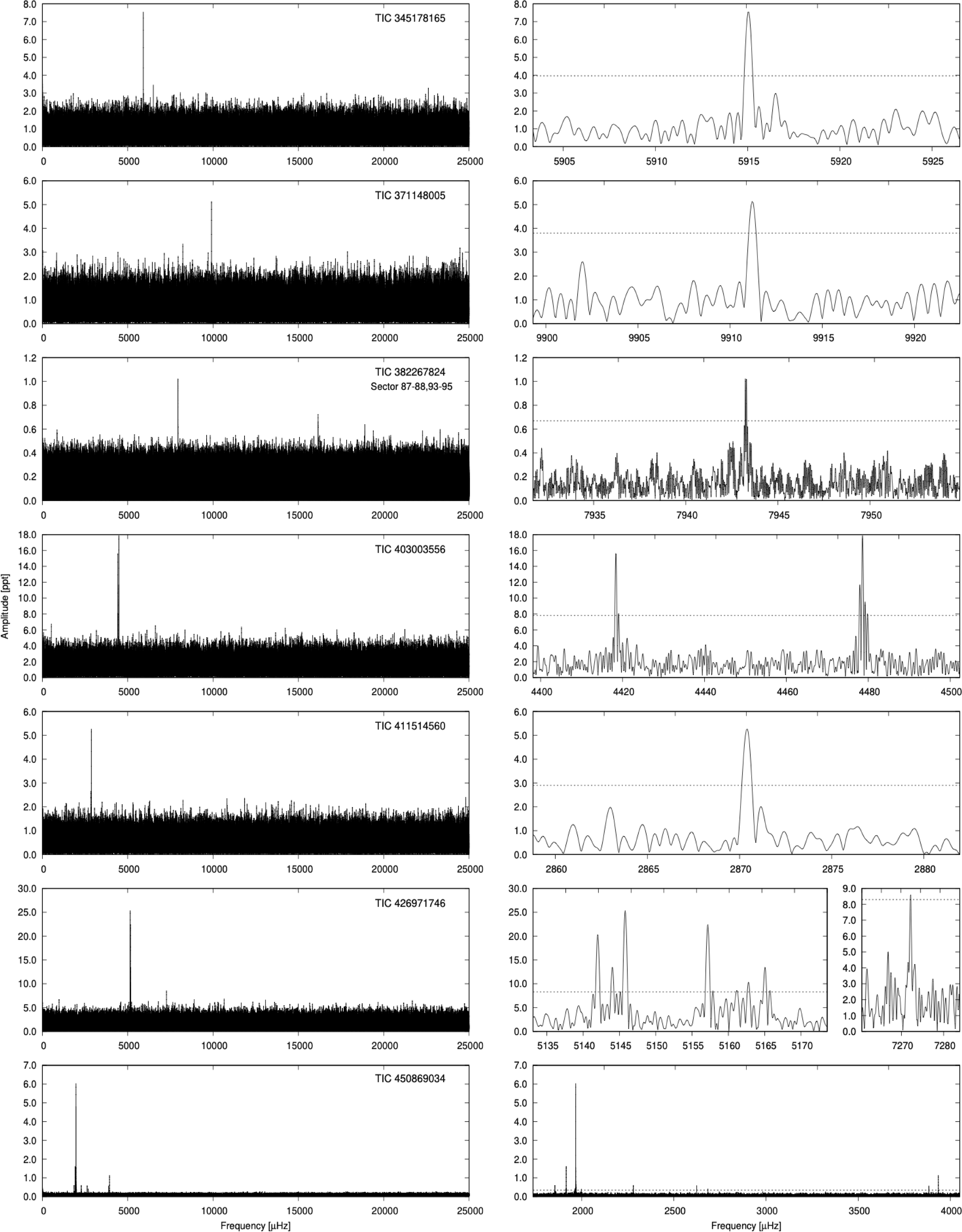
, which indicates an sdB type. TESS observed the star during Sector 90. We detected only one frequency in the p-mode region. We show the amplitude spectrum in Figure 4, and we list the prewhitened frequency in Table 3.
Amplitude spectra of targets observed in the USC mode. If sector is not specified, we included all USC data. As explained in Section 3 the ppt unit does not apply to TIC 450869034. Left panels: Frequency range up to the Nyquist frequency. Right panels: Close-ups of the detected frequencies.

Figure 4. Long description
The image contains multiple line graphs showing amplitude spectra of targets observed in the USC mode. Each target is represented by a pair of graphs: one showing the frequency range up to the Nyquist frequency and another providing a close-up of the detected frequencies. Panel A: The left graph for TIC 345178165 shows amplitude on the vertical axis and frequency in microhertz on the horizontal axis, with a notable peak around 5915 microhertz. The right graph zooms in on this frequency range, highlighting the peak. Panel B: The left graph for TIC 371148005 displays amplitude versus frequency, with a significant peak around 9910 microhertz. The right graph provides a detailed view of this frequency range. Panel C: The left graph for TIC 382267824 shows amplitude versus frequency, with a prominent peak around 7945 microhertz. The right graph zooms in on this frequency range. Panel D: The left graph for TIC 403003556 displays amplitude versus frequency, with a notable peak around 4440 microhertz. The right graph provides a detailed view of this frequency range. Panel E: The left graph for TIC 411514560 shows amplitude versus frequency, with a significant peak around 2870 microhertz. The right graph zooms in on this frequency range. Panel F: The left graph for TIC 426971746 displays amplitude versus frequency, with a prominent peak around 5160 microhertz. The right graph provides a detailed view of this frequency range. Panel G: The left graph for TIC 450869034 shows amplitude versus frequency, with a notable peak around 2000 microhertz. The right graph zooms in on this frequency range.
TIC 371148005 (Gaia DR3 896307108572160768) was not identified as a pulsator prior to the TESS mission. Wegner & Swanson (Reference Wegner and Swanson1990) classified the star as sdB. A spectrum we obtained with the NOT indicates an sdOB+G spectral classification. TESS observed the star during Sector 71 and we detected only one frequency in the p-mode region. We show the amplitude spectrum in Figure 4, and we list the prewhitened frequency in Table 3.
TIC 382267824 (Gaia DR3 4768581590363727616) was not identified as a pulsator prior to the TESS mission. O’Donoghue et al. (Reference O’Donoghue, Kilkenny, Koen, Hambly, MacGillivray and Stobie2013) classified the star as sdOB. A spectrum taken with the 1.9 m at SAAO indicates an sdOB+F/G classification. TESS observed the star during Sectors 27, 30, 31, 33–34, 37, 64–68, 87–88, 93–95. We detected no significant signal in an amplitude spectrum calculated from the combined dataset collected during Sectors 27, 30, 31, 33, 34, 37. However, we detected one frequency in the p-mode region in each of the combined datasets collected during Sectors 64–68 and 87–88, 93–95. The noise levels in these three distinct groups of sectors are very similar, which indicates variable amplitude of the pulsation – probable cause of the null detection in the early sectors. We show the amplitude spectrum calculated from the latter dataset in Figure 4, and we list the prewhitened frequency in Table 3.
TIC 403003556 (Gaia DR3 5830605541014576512) was not identified as a pulsator prior to the TESS mission. Based on the Gaia colour index
 $B_{p}-R_{p}=-0.26$
and absolute magnitude
 $G_\textrm{Mag}=4.66$
, the star is considered a hot subdwarf. TESS observed the star during Sector 93 and we detected two frequencies, both in the p-mode region. We show the amplitude spectrum in Figure 4, and we list the prewhitened frequencies in Table 3.
TIC 411514560 (Gaia DR3 2772359715502793088) was not identified as a pulsator prior to the TESS mission. Robinson & Winget (Reference Robinson and Winget1983) classified the star as a horizontal branch object. Pérez-Fernández et al. (Reference Pérez-Fernández, Ulla, Solano, Oreiro and Rodrigo2016) reclassified the star as a hot subdwarf with a
 $T_\textrm{eff}$
to be 27 000 K, which indicates an sdB type. From our fit to a spectrum taken with the NOT, we derived
 $T_\textrm{eff}=29\,873(149)$
K,
 $\log$
(g/
 $\mbox{cm}\,\mbox{s}^{-2}$
) = 5.44(2) and
 $\log$
(n(He)/n(H))
 $=-2.45(5)$
, which indicates an sdOB type. TESS observed the star during Sector 83 and we detected only one frequency in the p-mode region. We show the amplitude spectrum in Figure 4, and we list the prewhitened frequency in Table 3.
TIC 426971746 (Gaia DR3 6423384454599994880) was not identified as a pulsator prior to the TESS mission. Based on the Gaia colour index
 $B_{p}-R_{p}=-0.36$
and absolute magnitude
 $G_\textrm{ Mag}=4.52$
, the star is considered a hot subdwarf. TESS observed the star during Sector 93 and we detected eight frequencies, all in the p-mode region. We show the amplitude spectrum in Figure 4, and we list the prewhitened frequencies in Table 3. Frequencies
 $f_1-f_3$
are closely spaced together, with spacings of 1.95(30) and 1.86(32)
 $\unicode{x03BC}$
Hz. If these are rotationally induced split modes, the average rotation period is 6.08(26) days.
TIC 450869034 (Gaia DR3 5820575349265385600) was identified as a pulsator prior to the TESS mission. Borowicz et al. (Reference Borowicz2023) classified the star as a blue large amplitude pulsator. Pietrukowicz et al. (Reference Pietrukowicz2025) provided
 $T_\textrm{eff}$
,
 $\log$
(g/
 $\mbox{cm}\,\mbox{s}^{-2}$
) and
 $\log$
(n(He)/n(H)) to be 32 700(200) K, 5.28(3) and
 $-2.80(9)$
, respectively. TESS observed the star during Sectors 64–65 and we detected ten frequencies, with two being combination frequencies of the two largest amplitude frequencies. We show the amplitude spectrum in Figure 4, and we list the prewhitened frequency in Table 3. The amplitudes of flux variability are large but not too large for a pulsating hot subdwarf (e.g. Baran et al. Reference Baran2009). Moreover, the atmospheric parameters are well within the range for hot subdwarfs. Since this target could well be an sdB pulsator, we include it in our sample and we consider it to be a pulsating hot subdwarf star, until proven otherwise.
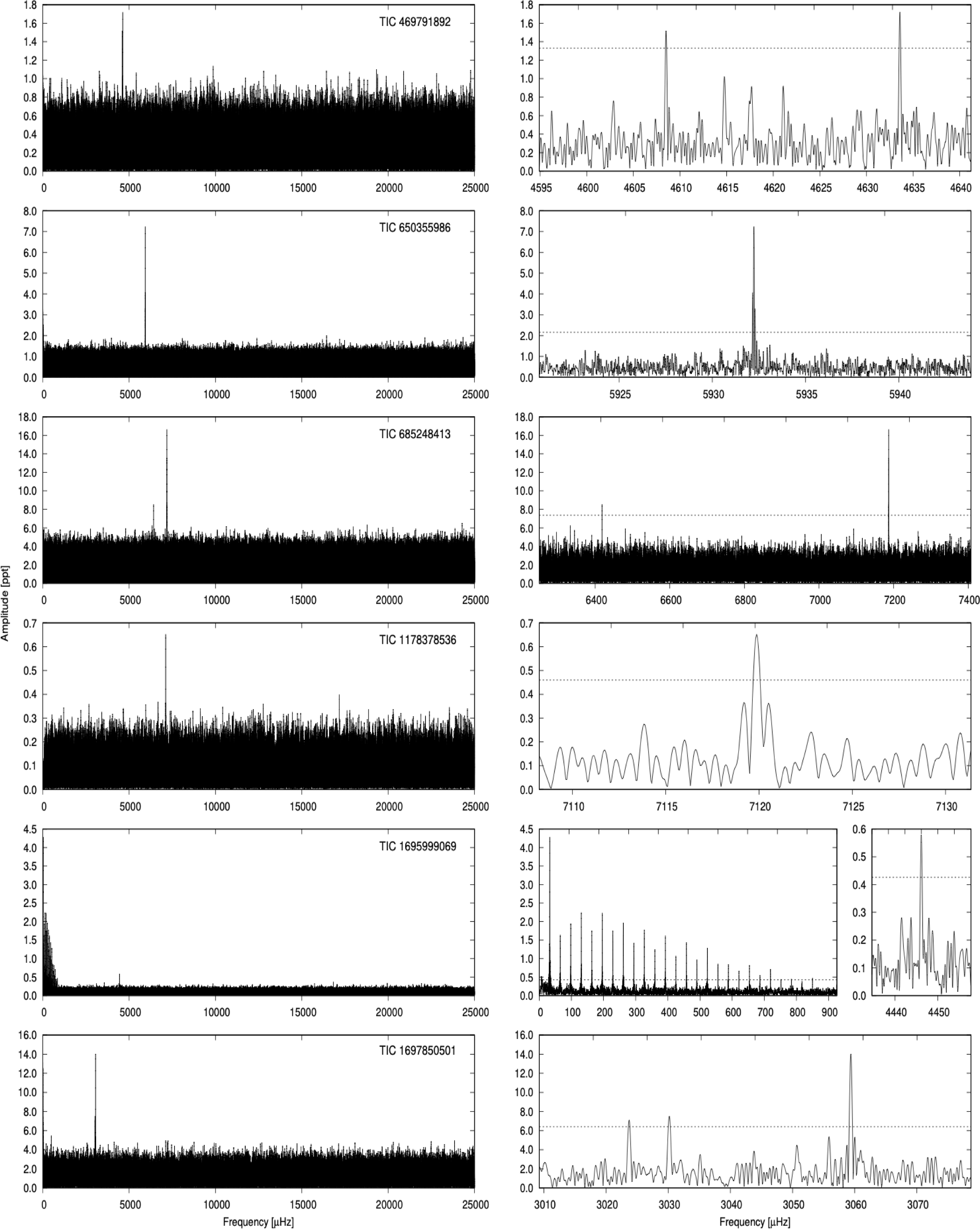
TIC 469791892 (Gaia DR3 6423384454599994880) was not identified as a pulsator prior to the TESS mission. O’Donoghue et al. (Reference O’Donoghue, Kilkenny, Koen, Hambly, MacGillivray and Stobie2013) classified the star as sdB. TESS observed the star during Sectors 93–94 and we detected two frequencies in the p-mode region. We show the amplitude spectrum in Figure 5, and we list the prewhitened frequencies in Table 3.
Amplitude spectra of targets observed in the USC mode. If sector is not specified, we included all USC data. As explained in Section 3 the ppt unit does not apply to TIC 1178378536 and TIC 1695999069. Left panels: Frequency range up to the Nyquist frequency. Right panels: Close-ups of the detected frequencies.

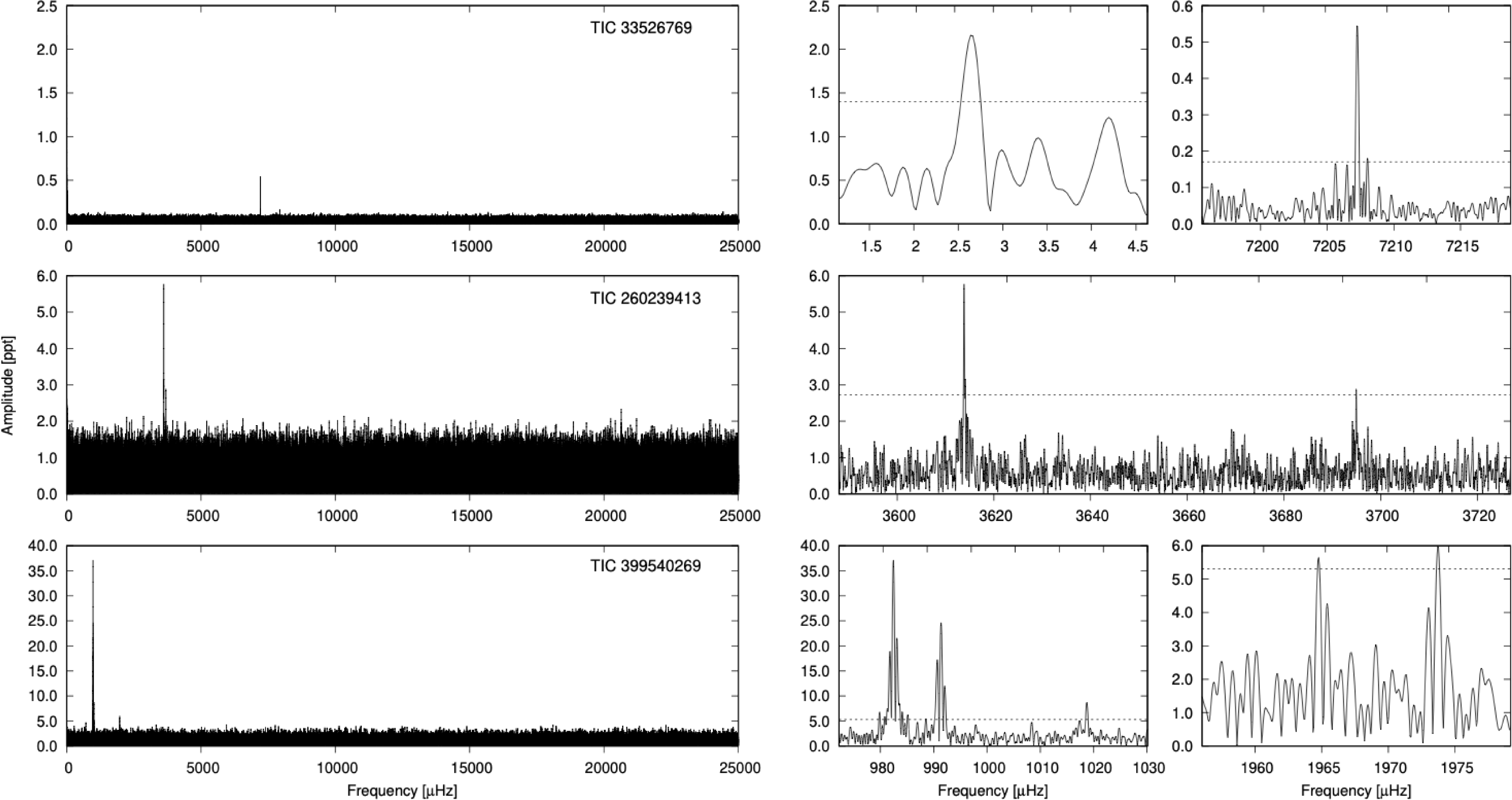
Amplitude spectra of two stars observed during Sector 97 (top two panels) and a BLAP star (bottom panel). Left panels: Frequency range up to the Nyquist frequency. Right panels: Close-ups of the detected frequencies. In case of TIC 33526769 only local frequency range was used to calculate the threshold dashed line for the
 $\Omega$
frequency.

Figure 6. Long description
The image contains six line graphs depicting amplitude spectra of stars observed during Sector 97 and a BLAP star. The graphs are organized into three rows, each with two panels. Panel A: The top left graph shows the amplitude spectrum for TIC 33526769. The x-axis represents frequency in microhertz (µHz) ranging from 0 to 25000, and the y-axis represents amplitude in parts per thousand (ppt) ranging from 0 to 2.5. The graph shows a relatively flat amplitude spectrum with a few small peaks. The top right graph is a close-up of the detected frequencies for TIC 33526769. The x-axis ranges from 7200 to 7215 µHz, and the y-axis ranges from 0 to 0.6 ppt. This graph shows a prominent peak around 7207 µHz. Panel B: The middle left graph shows the amplitude spectrum for TIC 260239413. The x-axis ranges from 0 to 25000 µHz, and the y-axis ranges from 0 to 6 ppt. The graph shows a relatively flat amplitude spectrum with a few small peaks. The middle right graph is a close-up of the detected frequencies for TIC 260239413. The x-axis ranges from 3600 to 3720 µHz, and the y-axis ranges from 0 to 6 ppt. This graph shows several prominent peaks, with the highest around 3620 µHz. Panel C: The bottom left graph shows the amplitude spectrum for TIC 399540269. The x-axis ranges from 0 to 25000 µHz, and the y-axis ranges from 0 to 40 ppt. The graph shows a relatively flat amplitude spectrum with a few small peaks. The bottom right graph is a close-up of the detected frequencies for TIC 399540269. The x-axis ranges from 980 to 1030 µHz and from 1960 to 1975 µHz, and the y-axis ranges from 0 to 6 ppt. This graph shows several prominent peaks, with the highest around 990 µHz and 1965 µHz.
TIC 650355986 (Gaia DR3 4667580383516276864) was not identified as a pulsator prior to the TESS mission. From our fit to a spectrum taken with the 1.9 m telescope at SAAO, we derived
 $T_{\rm eff}=30\,790(191)$
K,
 $\log$
(g/
 $\mbox{cm}\,\mbox{s}^{-2}$
) = 6.05(7) and
 $\log$
(n(He)/n(H)) =
 $-1.94(9)$
, which indicates an sdB type. TESS observed the star during Sectors 87–90, 93–96 and we detected only one frequency in the p-mode region in all-sector combined dataset. We show the amplitude spectrum in Figure 5, and we list the prewhitened frequency in Table 3.
TIC 685248413 (Gaia DR3 4774297672143006592) was not identified as a pulsator prior to the TESS mission. From our fit to a spectrum taken with the 1.9 m telescope at SAAO, we derived
 $T_\textrm{eff}=34\,477(757)$
K,
 $\log$
(g/
 $\mbox{cm}\,\mbox{s}^{-2}$
) = 5.73(17) and
 $\log$
(n(He)/n(H)) =
 $-1.81(23)$
, which indicates an sdB type. Kilkenny et al. (Reference Kilkenny, O’Donoghue, Worters, Koen, Hambly and MacGillivray2015) classified the star as sdB. TESS observed the star during Sectors 89–90, 93–96. We detected two frequencies in the p-mode region in an all-sector combined dataset. We show the amplitude spectrum in Figure 5, and we list the prewhitened frequencies in Table 3.
TIC 1178378536 (Gaia DR3 6257666302578107008) was found to be a pulsator prior to the TESS mission by Kilkenny et al. (Reference Kilkenny, Worters, O’Donoghue, Koen, Koen, Hambly, MacGillivray and Stobie2016) who reported three significant frequencies. Kilkenny et al. (Reference Kilkenny, O’Donoghue, Koen, Stobie and Chen1997b) classified the star as sdB. From our fit to a spectrum taken with the NOT, we derived
 $T_\textrm{eff}=33\,727(153)$
K,
 $\log$
(g/
 $\mbox{cm}\,\mbox{s}^{-2}$
) = 5.72(3) and
 $\log$
(n(He)/n(H)) =
 $-1.47(4)$
, which indicates an sdOB type. TESS observed the star during Sector 91. We detected only one frequency in the p-mode region, which overlaps with the dominant amplitude signal reported by Kilkenny et al. (Reference Kilkenny, Worters, O’Donoghue, Koen, Koen, Hambly, MacGillivray and Stobie2016). Assuming the same amplitude ratio between the signal detected by Kilkenny et al. (Reference Kilkenny, Worters, O’Donoghue, Koen, Koen, Hambly, MacGillivray and Stobie2016), the other two frequencies would be below the detection threshold in TESS datasets analysed in this work. We show the amplitude spectrum in Figure 5, and we list the prewhitened frequency in Table 3.
TIC 1695999069 (Gaia DR3 6720657317455798400) was not identified as a pulsator prior to the TESS mission. Sahoo et al. (Reference Sahoo, Baran, Sanjayan and Ostrowski2020) found it to be an eclipsing binary with an orbital period of 0.3536 days. Worters et al. (Reference Worters, Kilkenny, Nemeth, Baran and Østensen2026) reported
 $T_\textrm{eff}=32\,930(680)$
K,
 $\log$
(g/
 $\mbox{cm}\,\mbox{s}^{-2}$
) = 5.93(10) and
 $\log$
(n(He)/n(H)) =
 $-2.50(26)$
, which indicates an sdB type. TESS observed the star during Sector 93. We detected two frequencies, with the dominant one at half the orbital frequency reported by Sahoo et al. (Reference Sahoo, Baran, Sanjayan and Ostrowski2020), and the other in the p-mode region. We show the amplitude spectrum in Figure 5 and we list the prewhitened frequencies in Table 3.
TIC 1697850501 (Gaia DR3 6723398326932092032) was not identified as a pulsator prior to the TESS mission. Based on the Gaia colour index
 $B_{p}-R_{p}=-0.05$
and absolute magnitude
 $G_\textrm{ Mag}=4.45$
, the star is considered a hot subdwarf. TESS observed the star during Sector 93 and we detected three frequencies, all in the p-mode region. There may also be a real signal at a very low frequency that would correspond to a period of 0.7 day. If the signal is intrinsic to the star (we can rule out any contamination), it indicates binarity. We show the amplitude spectrum in Figure 5, and we list the prewhitened frequencies in Table 3.
4.1. Two pulsating hot subdwarfs detected in Sector 97
Even though our main focus was on Years 5–7 of TESS – which are already completed – while working on this paper, we took advantage of the very first sector of Year 8, which was already accessible and added the following two stars observed in Sector 97 (during Year 8) of the TESS mission.
TIC 33526769 (Gaia DR3 5025362802928256640, SB 744) was not identified as a pulsator prior to the TESS mission. TESS observed the star during Sector 97. We detected two frequencies in the p-mode region, and one very low frequency. The latter cannot be associated with g-modes, hence, if real, it may be a signature of the rotation of the main sequence component. We show the amplitude spectrum in Figure 6, and we list the prewhitened frequencies in Table 3. This star is the first case of its kind, specifically, it is the very first p-mode dominated heavy-metal hot subdwarf star. The star was found to be the sdOB+F/G binary consisting of the hot subdwarf component identified as a heavy-metal star (Németh et al. Reference Németh, Vos, Molina and Bastian2021). There are three other heavy-metal hot subdwarfs, so-called V366 Aquarid stars, reported thus far (Ahmad & Jeffery Reference Ahmad and Jeffery2005; Latour et al. Reference Latour, Green and Fontaine2019; Østensen et al. Reference Østensen2020), however they are all g-mode dominated, while TIC 33526769 is p-mode dominated.
TIC 260239413 (Gaia DR3 5482554001345846272) was not identified as a pulsator prior to the TESS mission. From our fit to a spectrum taken with the 1.9 m telescope at SAAO, we derived
 $T_\textrm{eff}=31\,178(235)$
K,
 $\log{(\mathrm{g}/{\mbox{cm}\,\mbox{s}^{-2}})}\,=\,5.65(6)$
and
 $\log$
(n(He)/n(H)) =
 $-3.27(16)$
, which indicates an sdB type. Kilkenny et al. (Reference Kilkenny, O’Donoghue, Worters, Koen, Hambly and MacGillivray2015) classified the star as sdB. TESS observed the star during Sector 97. We detected two frequencies in the p-mode region. We show the amplitude spectrum in Figure 6, and we list the prewhitened frequencies in Table 3.
4.2 An unusual blue large-amplitude pulsator
TIC 399540269 (Gaia DR3 4139067134284899456) was detected to have strong peaks around 1 000
 $\unicode{x03BC}$
Hz, and therefore flagged for follow-up spectroscopy. The main mode has an amplitude that reaches 3.7%, which is very high for any hot subdwarf pulsator. Our spectrum taken with the NOT revealed that the target is an unusual blue star. The surface gravity is certainly lower than the classic sdB limit of
 $\log$
 $g\lt 5.0$
dex, and therefore outside the limits of our model grid. We roughly extrapolated physical parameters to be
 $T_\textrm{eff}=27\,500\,K$
,
 $\log{(\mbox{g}/{\mbox{cm}\,\mbox{s}^{-2}})}\,=\,4.7$
, and
 $\log$
(n(He)/n(H))
 $=-0.6$
. This places the object in a sparsely populated part of the parameter space, well above the Extreme Horizontal Branch, and well below the Main Sequence. The object was identified as a blue large-amplitude pulsator (BLAP) in the sample of hot subdwarfs observed in the course of the Zwicky Transient Facility survey (Kupfer et al. Reference Kupfer2021). It was found to be a single mode pulsator with an amplitude of 37.3 mmag and a pulsation period of 995.479 s. TESS observed the star during Sector 91. We detected five frequencies. The two highest frequencies may actually be combinations of the two frequencies with the highest amplitudes, i.e.
 $f_4=2\cdot f_1$
and
 $f_5=f_1+f_2$
. None of the frequencies we detected corresponds strictly to the one reported in the literature, while the amplitude of the highest amplitude frequency in our work agrees with the one reported in the literature. This star cannot be considered a single mode pulsator (Kupfer et al. Reference Kupfer2021) any longer. We show the amplitude spectrum in bottom panel of Figure 6, and we list the prewhitened frequencies in Table 3.
5. SC targets re-observed in the USC mode
Twenty four targets included in work by Baran et al. (Reference Baran2023) and (2024) were observed in the SC mode in TESS years 1–4. Once they were found to be pulsators, the majority of these targets, specifically 20 out of 24, were re-observed in the USC mode, to ensure that the pulsation spectrum is identified properly, and potentially to detect more p-mode frequencies. As mentioned by Baran et al. (Reference Baran2023) the Nyquist frequency in the SC mode happens to be in the middle of the p-mode range for hot subdwarfs and signals can be mirrored across the Nyquist frequency, preventing a proper identification of a signal. As shown by Baran et al. (Reference Baran2012) such a crossover can be disentangled when data are collected over a substantial part of Earth’s orbit. In the case of TESS many stars are observed during single sectors, so the disentangling technique is hardly applicable.
Our main intention to re-analyse those SC targets, now re-observed in the USC mode, is to update Figures 5 and 6 originally presented by Baran et al. (Reference Baran, Charpinet, Østensen, Reed, Van Grootel, Lyu, Telting and Németh2024). To be consistent with Baran et al. (Reference Baran, Charpinet, Østensen, Reed, Van Grootel, Lyu, Telting and Németh2024), for this part of our work, we accepted amplitudes that satisfy S/N
 $\geq$
4.5, but frequencies with S/N
 $\leq$
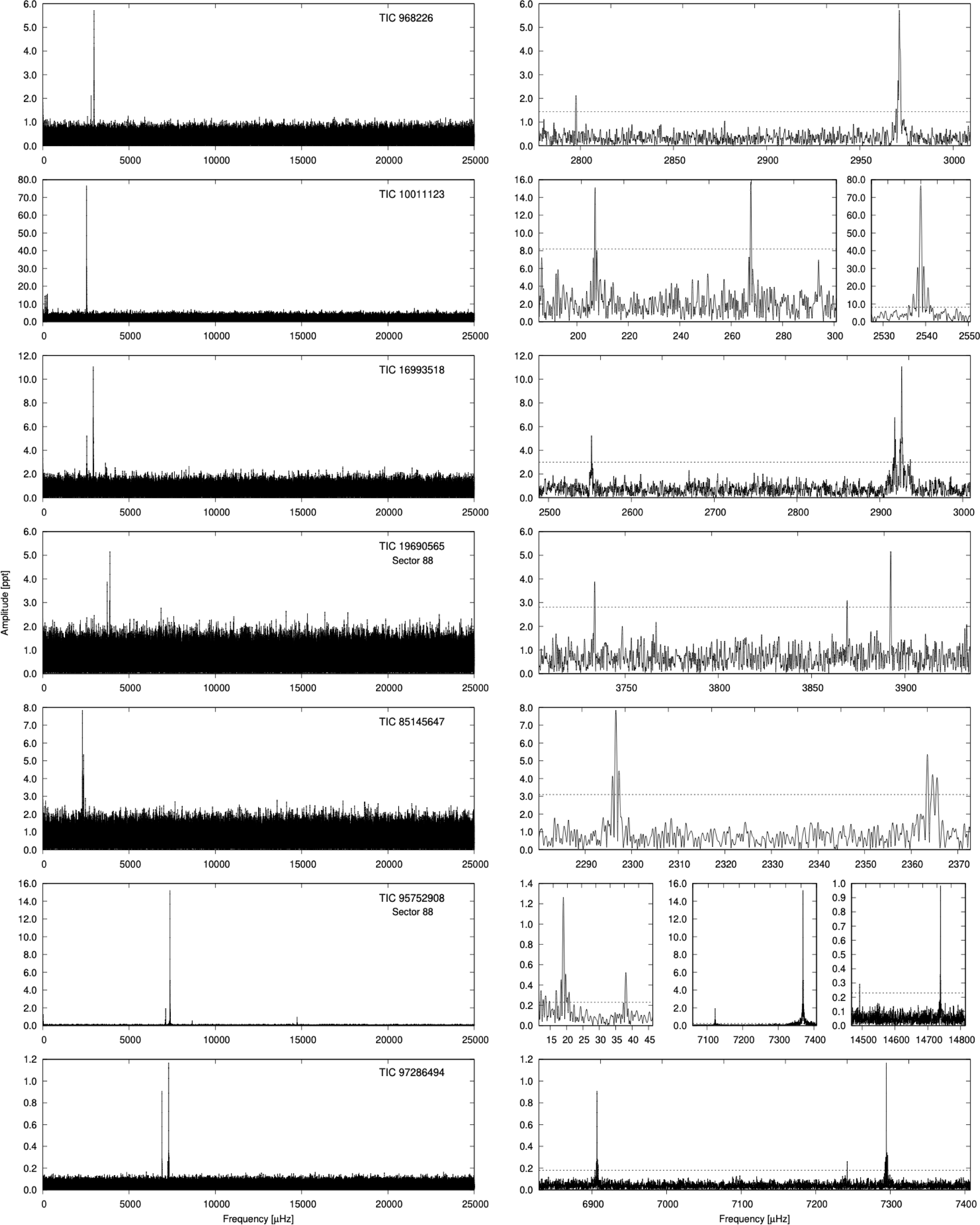
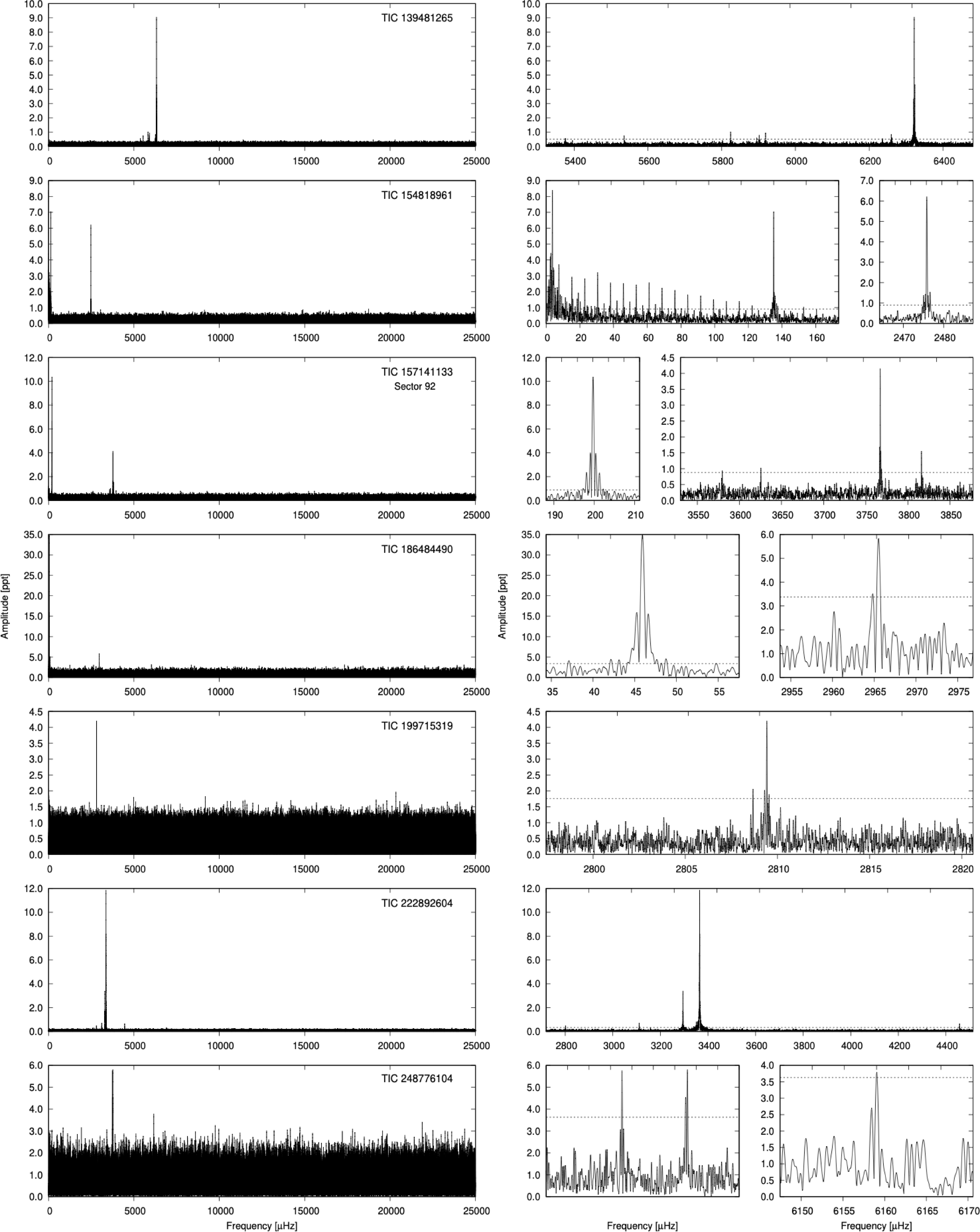
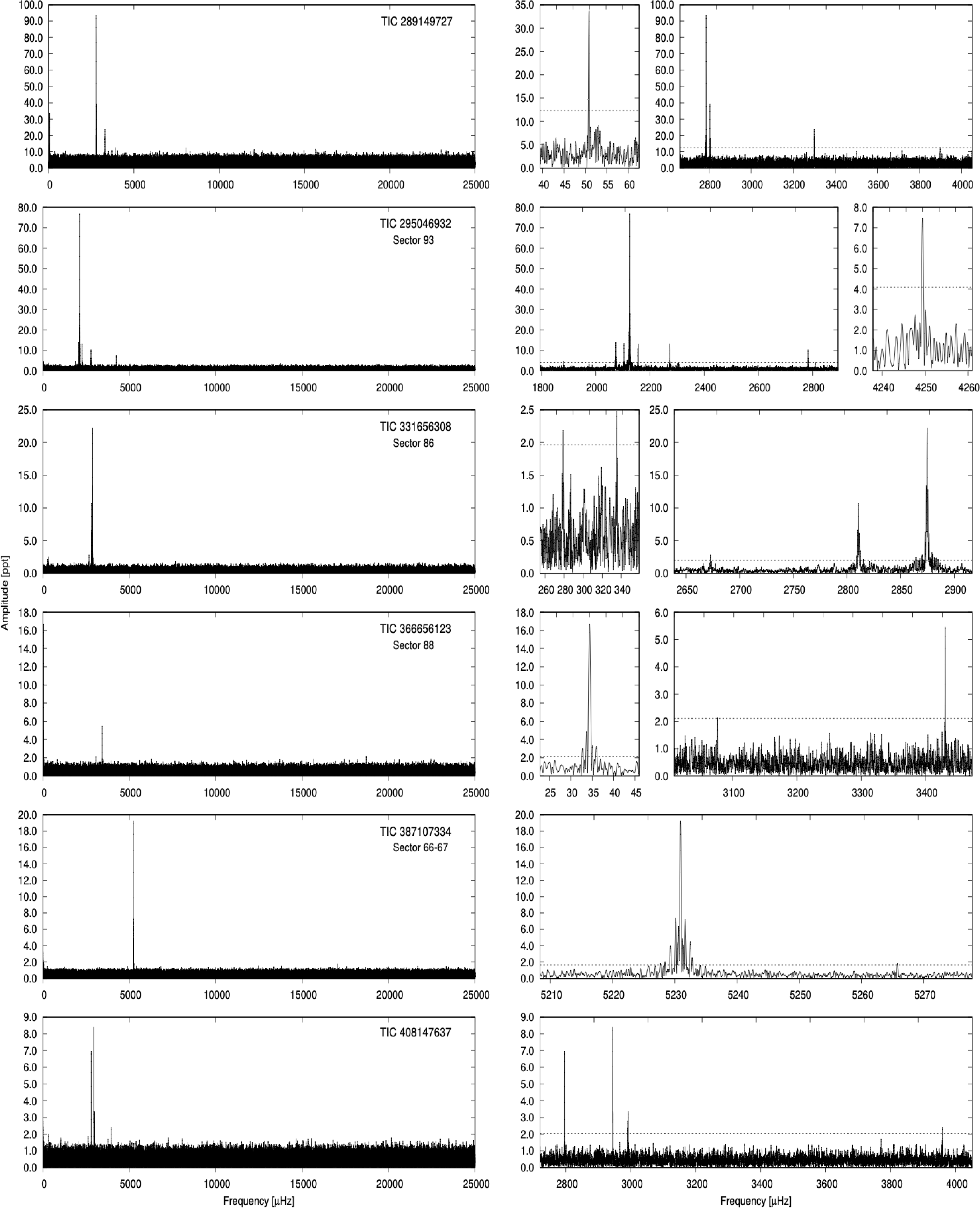
5.5 should always be considered tentative. We do not describe the targets in individual paragraphs, however, below we provide a summary of our analysis of the USC data. The significant frequencies are listed in Table 4 (the SC data); we included sector numbers for each analysed star/dataset. We show the amplitude spectra in Figures 7–9.
List of frequencies detected in the previously analysed SC targets, now re-observed in the USC.

Table 4. Long description
Panel A: Line graph displaying amplitude spectra with frequency on the x-axis in microhertz and amplitude on the y-axis in parts per million. Panel B: Line graph showing another set of amplitude spectra with similar axes. Panel C: Line graph with frequency on the x-axis and amplitude on the y-axis, highlighting significant frequencies.
One star in this sample needs a spectroscopic correction. TIC 10011123 was reported by Baran et al. (Reference Baran2023) as sdOB. According to Worters et al. (Reference Worters, Kilkenny, Nemeth, Baran and Østensen2026) the star is classified as an sdB. Our final statistics will reflect this update. Two stars, i.e. TIC 392092589 and TIC 455095580, show no significant signal. The former star was observed during Sectors 71–72 whereas the latter was observed during Sectors 61 and 88. TIC 392092589 was reobserved in the USC during one sector only, however if the amplitudes of the modes have not changed, three out of four frequencies should still be detectable, even given about 30% higher average noise level. In the SC mode TIC 455095580 was observed during one sector only. In the case of both stars the lack of signal can be explained by the amplitude change. In case of 13 stars, the USC data confirmed the right choice of either sub- or super-Nyquist frequencies made by Baran et al. (Reference Baran2023, Reference Baran, Charpinet, Østensen, Reed, Van Grootel, Lyu, Telting and Németh2024). For seven stars (TICs: 10011123, 16993518, 19690565, 222892604, 289149727, 295046932, 408147637) the reported SC frequencies happened to be aliases across Nyquist; the true frequencies originate from the sub-Nyquist region. It is well known that amplitudes of pulsations in hot subdwarfs are variable (see, for example, Kilkenny Reference Kilkenny2010), therefore we checked to see if the highest amplitude modes remained the same or changed, and in the case of change, how different the frequencies are. The latter could have a strong impact on the relationship between asteroseismic and atmospheric parameters discussed in Section 6. If only one solution is given for both the previously reported SC and USC data analysed here, the comparison is fairly easy. In case of multiple solutions, the outcome of the comparison may depend on the solutions considered. For 12 stars we find that the modes with the highest amplitude modes remained the same. In case of four stars the modes with the highest amplitudes changed. While for the remainder, i.e. three stars, it depends on which sectors we compared. We did account for a super- to sub-Nyquist swap. In neither case listed above was the frequency change large enough to influence the picture of the analysis presented in Section 6. Since the noise level in an amplitude spectrum calculated either from the SC or USC data should roughly stay the same (assuming both datasets are roughly complete and taken over comparable timespan), we do not expect the USC data alone to be the cause of more or fewer frequencies detected. We preserved the same detection threshold, so any significant change in a number of detected frequencies will probably come from the intrinsic behaviour of stars. This statement remains valid as long as we are not considering frequencies close to the Nyquist frequency or its multiples. For the majority of stars, we found roughly the same number of frequencies are reported by Baran et al. (Reference Baran2023, Reference Baran, Charpinet, Østensen, Reed, Van Grootel, Lyu, Telting and Németh2024). For some of those stars there is a gain or loss of one or two frequencies. There are a few stars that show exceptionally different frequency content compared to the results from the SC data. TIC 95752908 shows more pulsation modes along with combination frequencies, as well as a binary signature. The latter two features were not detected in the SC data. In TIC 97286494 we found four frequencies, while only one was reported prior. For TIC 139481265, the increase in the number of frequencies is substantial, i.e. only three detected in the SC data whereas 13 in the USC data. Depending on a Sector, for TIC 295046932, the increase is either by one or six frequencies.
6. Discussion
Following TESS Sector 60 (at the end of TESS year 4), we found another 36 p-mode pulsating hot subdwarfs, including 20 sdB and 10 sdOB stars, one eHe-sdOB star, and five stars that are classified as hot subwarfs of yet undefined type. Only three pulsators in our sample were known prior to the TESS mission. Overall, including the results of the search in both ecliptic hemispheres reported by Baran et al. (Reference Baran2023, Reference Baran, Charpinet, Østensen, Reed, Van Grootel, Lyu, Telting and Németh2024), p-mode pulsations in 129 hot subdwarfs observed by TESS were found. Another star reported by Baran et al. (Reference Baran2023) needs a spectroscopic update. TIC 60257911 was reported by the authors as sdB, in accordance to previous findings, while Lei et al. (Reference Lei, He, Németh, Vos, Zou, Hu, Xiao, Yan and Zhao2023) classified it as an sdOB. That being said, we now count this star as an sdOB, so the final sample includes 86 sdB, 34 sdOB, two sdO, two He-sdOB stars, and five stars of yet undetermined types.
Amplitude spectra of SC targets re-observed in the USC mode. Left panels: Frequency range up to the Nyquist frequency. Right panels: Close-ups of the detected frequencies. We show only one amplitude spectrum per star. In case of multiple solutions for a given star provided in Table 4 the Sector(s) number is also added.

Amplitude spectra of SC targets re-observed in the USC mode. Left panels: Frequency range up to the Nyquist frequency. Right panels: Close-ups of the detected frequencies. We show only one amplitude spectrum per star. In case of multiple solutions for a given star provided in Table 4 the Sector(s) number is also added.

Figure 8. Long description
The image contains multiple line graphs depicting amplitude spectra of various stars re-observed in the USC mode. Each row represents a different star, with two panels per row. Panel A on the left shows the frequency range up to the Nyquist frequency, while Panel B on the right provides close-ups of the detected frequencies. Each graph has amplitude on the vertical axis and frequency in microhertz (uHz) on the horizontal axis. The stars are identified by their TIC numbers, and some graphs include sector numbers indicating multiple solutions for a given star. Notable trends include prominent peaks at specific frequencies, indicating significant amplitude at those points. The graphs vary in the number and height of peaks, reflecting the different characteristics of each star‘s amplitude spectrum.
Amplitude spectra of SC targets re-observed in the USC mode. Left panels: Frequency range up to the Nyquist frequency. Right panels: Close-ups of the detected frequencies. We show only one amplitude spectrum per star. In case of multiple solutions for a given star provided in Table 4 the Sector(s) number is also added.

Atmospheric parameters for 108 stars out of 129 stars, presented in Baran et al. (Reference Baran2023, Reference Baran, Charpinet, Østensen, Reed, Van Grootel, Lyu, Telting and Németh2024) and this work, are listed in Table 2. It does not represent a uniform sample, since the parameters were derived either with the non-local thermodynamic equilibrium (NLTE) or local thermodynamic equilibrium (LTE) models. There is an expected systematic shift between LTE and NLTE that increases at higher temperature. That is why the LTE models are not calculated for
 $T_\textrm{eff}$
higher than 40 000 K. Both models are comparable for
 $T_\textrm{eff}$
below 30 000 K and become progressively worse above this temperature.
LTE models overpopulate higher energy levels and therefore systematically overestimate
 $T_\textrm{eff}$
compared to NLTE models by 1 000–2 000 K. Because NLTE lowers the ionisation fraction in the line-forming regions, the equivalent widths of Balmer lines change. Consequently, LTE models typically yield surface gravities that are underestimated by 0.1–0.2 dex compared to NLTE results. In cases discussed in Sections 6.2 and 6.3 the systematics between NLTE and LTE models do not matter much, since we are only looking for rough trends and the intrinsic scatter is dominant.
Four stars in Table 2 have spectroscopic parameters reported prior, while we refer to the work by Worters et al. (Reference Worters, Kilkenny, Nemeth, Baran and Østensen2026). TIC 6116091, parameters were included in Baran et al. (Reference Baran2023) but they were derived from UVES spectra and no uncertainties were given, so we used the values from Worters et al. (Reference Worters, Kilkenny, Nemeth, Baran and Østensen2026). TIC 62381958 – parameters reported by Worters et al. (Reference Worters, Kilkenny, Nemeth, Baran and Østensen2026) are comparable with the ones reported by Baran et al. (Reference Baran, Charpinet, Østensen, Reed, Van Grootel, Lyu, Telting and Németh2024). TIC 241771689 and TIC 471013461 –
 $T_\textrm{eff}$
and
 $\log$
g reported by Worters et al. (Reference Worters, Kilkenny, Nemeth, Baran and Østensen2026) have smaller uncertainties compared to those reported previously.
6.1. Summary of our discovery of new, or revision of previously reported, pulsating hot subdwarf stars
We report the discovery of the first known pulsating helium enhanced sdOB star, TIC 323572215. As pointed out by Sahoo et al. (Reference Sahoo, Baran, Worters, Németh and Kilkenny2023), such pulsators were unknown prior to the TESS mission, and our discovery indicates that the enhanced helium abundance does not prevent hot subdwarfs from pulsating, contrary to previous assumptions. This finding completes the known range of hot subdwarf pulsators across all atmospheric helium contents, which should be included in studies related to the driving mechanism in hot subdwarfs.
One of the objects, TIC 33526769, is the first p-mode-dominated sdOB in a binary system, identified as a heavy metal star. In contrast, three previously known similar stars – V366 Aqr stars – were all g-mode-dominated (Ahmad & Jeffery Reference Ahmad and Jeffery2005; Latour et al. Reference Latour, Green and Fontaine2019; Østensen et al. Reference Østensen2020). Theoretical studies of V366 Aqr stars must now account for both types of pulsations.
The next interesting object is TIC 399540269, which lies outside the typical surface gravity range of hot subdwarfs and is located in a sparsely populated part of the Hertzsprung–Russell diagram. We detected multiple pulsation modes in this star, removing it from the single-mode blue large-amplitude pulsator definition previously reported by Kupfer et al. (Reference Kupfer2021).
Another object that deserves special attention is TIC 450869034. It was previously classified as a BLAP, primarily based on a relatively large pulsation amplitude. However, the spectrum reported by Pietrukowicz et al. (Reference Pietrukowicz2025) shows a typical sdB or sdOB classification. For a star to be classified as a high gravity BLAP, the amplitude must exceed what is typically observed in hot subdwarf pulsators; otherwise, they present as the same class. To discuss amplitudes, a comparison with another high amplitude hot subdwarf, such as V585 Peg (Baran et al. Reference Baran, Pigulski, Kozieł, Ogłoza, Silvotti and Zoła2005) is appropriate. TIC 450869034 has also a sufficiently low gravity that it resembles objects discussed in previous papers as either true Extreme Helium-Burning (EHB) stars or post-EHB stars, such as V338 Ser (Holdsworth et al. Reference Holdsworth, Østensen, Smalley and Telting2017) and GALEX J201337.6+092801 (Østensen et al. Reference Østensen2011). In fact, GALEX J201337.6+092801 has
 $T_\textrm{eff}=32\,100(1000)$
K,
 $\log$
(g/
 $\mbox{cm}\,\mbox{s}^{-2}$
) = 5.15(20), and
 $\log$
(n(He)/n(H)) =
 $-2.8(2)$
, which overlaps with the values for TIC 450869034 within the uncertainties. As discussed by Østensen et al. (Reference Østensen2011), low surface gravity indicates that a star is either a post-EHB (shell-He burning) object or a WD+WD merger product (core-He burning).
Lastly, two stars were spectroscopically reclassified. A spectral classification of sdB is adopted for TIC 10011123, while sdOB is adopted for TIC 60257911.
6.2. Evolutionary status and instability strip
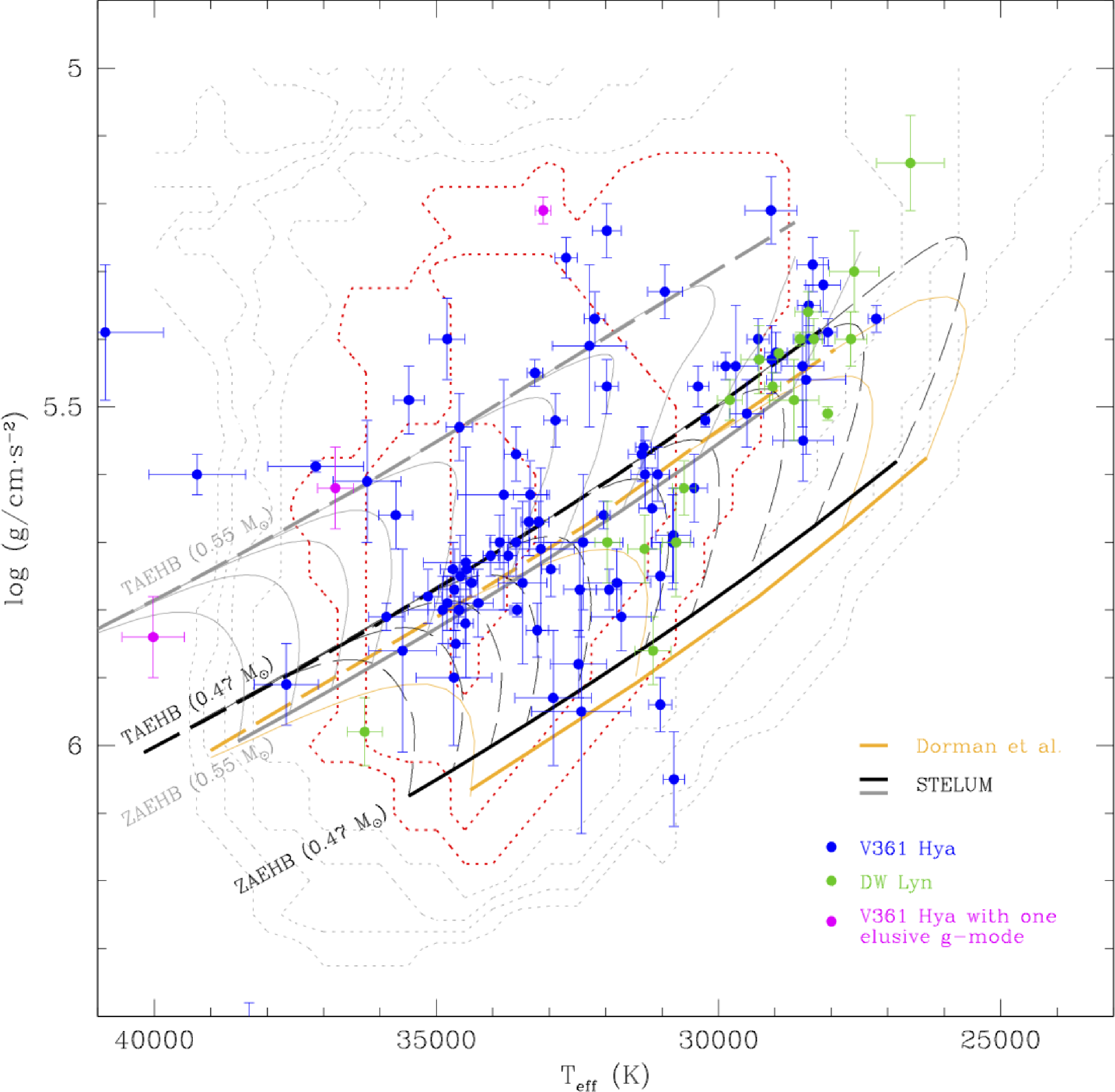
Figure 10 provides an updated version of Figure 4 of Baran et al. (Reference Baran, Charpinet, Østensen, Reed, Van Grootel, Lyu, Telting and Németh2024) showing the distribution, in the Kiel-diagram, of p-mode and hybrid hot subdwarf pulsators monitored by TESS up to Sector 97. The increased sample improves both the mapping of the instability region where p-mode pulsations are found and the comparison with evolutionary tracks and the theoretical instability strip derived from non-adiabatic pulsation calculations. We refer the reader to the detailed discussion of Baran et al. (Reference Baran, Charpinet, Østensen, Reed, Van Grootel, Lyu, Telting and Németh2024), which is still valid for this updated version. We simply point out four objects now tagged as hybrid pulsators, which – if confirmed – would greatly extend the range where such stars are typically found and challenge our understanding of the instability regions. Three of them (TIC 62381958, TIC 273255412, and TIC 295046932; magenta symbols in Figure 10) are detections of a single low-frequency signal slightly above our detection threshold and should therefore be regarded as tentative. The fourth star (also included in Figure 10) is TIC 241771689, which features, beyond any doubt, a fairly rich spectrum of both p- and g-modes, yet has atmospheric parameters (
 $T_\textrm{eff}$
 $\sim$
36 270 K and
 $\log$
(g/
 $\mbox{cm}\,\mbox{s}^{-2}$
) around 5.98) well outside the usual range for hybrid pulsators. These parameters were reported by Worters et al. (Reference Worters, Kilkenny, Nemeth, Baran and Østensen2026) and have smaller uncertainties compared to those reported previously. The short periods of the detected p-modes indeed suggest a fairly high surface gravity, while the presence of a very cool and faint companion should hardly affect the spectrum and the determination of the effective temperature (Kawka et al. Reference Kawka, Vennes, O’Toole, Németh, Burton, Kotze and Buckley2015; Németh et al. Reference Németh, Kawka and Vennes2012). The star is in a relatively crowded field and contamination could be an issue, but examination of the pixel data indicate that the pulsation signal (both low and high frequencies) are from TIC 241771689. Undoubtedly, this puzzling object will deserve special attention in future studies.
Distribution of p-mode hot-subdwarf pulsators observed by TESS (up to sector 97) in the Kiel diagram. Pure p-mode pulsators (V361 Hya stars) are shown as blue dots, while hybrid pulsators (also displaying g-modes – DW Lyn stars) are represented by green dots. Overlaid on this sample are the ZAEHB and TAEHB positions for assumed core masses of 0.47 M
 $_{\odot}$
(black curves) and 0.55 M
 $_{\odot}$
(grey curves), illustrating the dependence of the EHB location on stellar mass. The EHB tracks are computed using the STELUM code for the specified core masses and varying envelope masses, with D(H)
 $\equiv$
 $\log$
[Menv/(Mcore + Menv)] values ranging from –6.0 to –2.0 (from high to low
 $T_\textrm{eff}$
see (see Baran et al. Reference Baran, Charpinet, Østensen, Reed, Van Grootel, Lyu, Telting and Németh2024, for details). For comparison, typical 0.47 M
 $_{\odot}$
tracks assuming a solar uniform envelope composition are also shown (yellow curves; Charpinet et al. Reference Charpinet, Fontaine, Brassard and Dorman2000; Dorman et al. Reference Dorman, Rood and O’Connell1993). The background dotted-line contours represent the predicted number of excited
 $\textit l$
= 0 p-modes from non-adiabatic pulsation calculations, serving as a proxy for the
 $\kappa$
– mechanism efficiency (Charpinet et al. 2001). The three innermost contours (highlighted in red) outline the region of the
 $\log$
g –
 $T_\textrm{eff}$
plane where p-mode driving is strongest.

6.3. Pulsation periods vs
 $T_\textrm{eff}$
and
$\log\,g$


As reported by Charpinet et al. (Reference Charpinet, Fontaine, Brassard and Dorman2002) pulsation periods of p-modes show a relation with
 $T_\textrm{eff}$
and
 $\log\,g$
. In the case of non-radial modes, their behaviour depends on both modal degree and radial order and is noticeable for
 $T_\textrm{eff}$
and
 $\log\,g$
. Radial modes are only affected by
 $\log\,g$
. Baran et al. (Reference Baran, Charpinet, Østensen, Reed, Van Grootel, Lyu, Telting and Németh2024) showed two diagrams to investigate if such a correlation between pulsation periods and model atmospheric parameters can be established observationally.
In Figure 9 of Charpinet et al. (Reference Charpinet, Fontaine, Brassard and Dorman2002), results for radial (
 $l=0$
) and non-radial (
 $l=1,2,3$
) modes of radial orders
 $k=0, 1$
and 10 are presented. Pulsation periods of radial modes do not depend much on
 $T_\textrm{eff}$
while they are strongly and monotonically affected by
 $\log\,g$
. For non-radial modes, both the temperature and gravity can influence the pulsation periods. These change more rapidly with temperature for low radial order cases, and with surface gravity for higher radial order cases. Modal degree does not influence pulsation periods significantly.
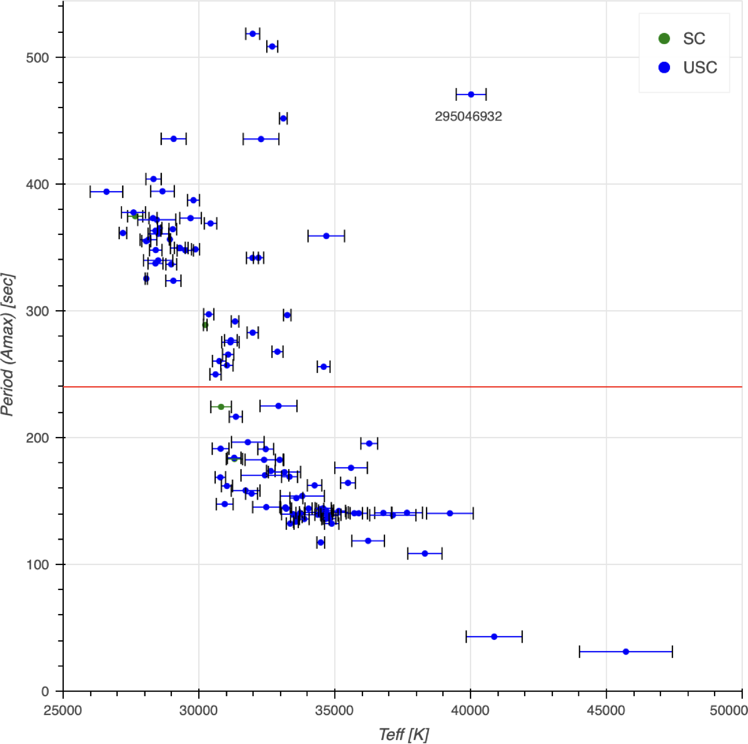
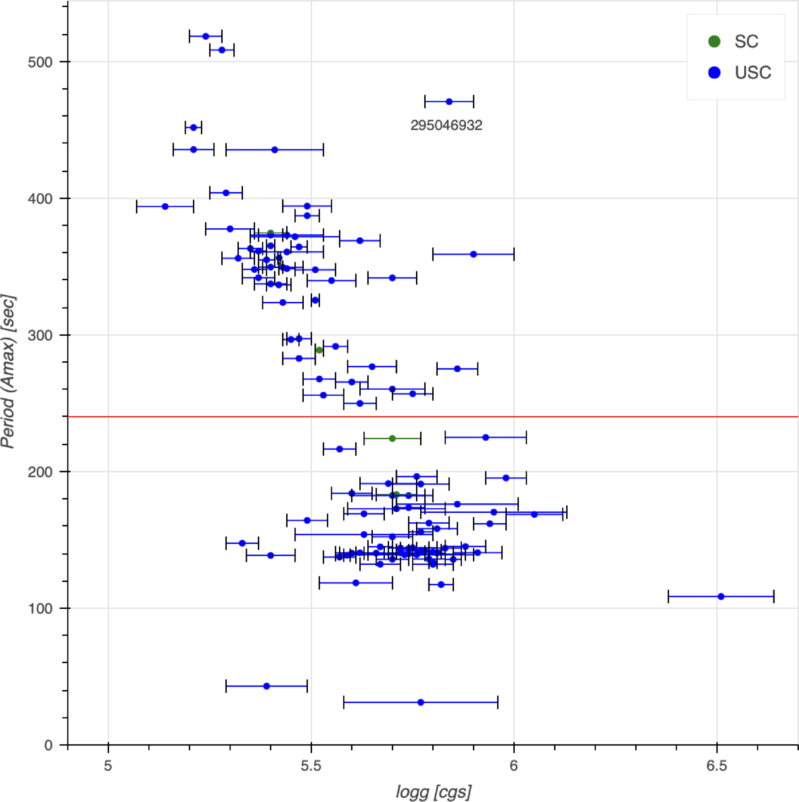
Only four stars were still unobserved in the USC mode, therefore the majority of them have pulsation frequencies not affected by the ambiguity of aliasing across the Nyquist frequency. This is a substantial update from Figures 5 and 6 in Baran et al. (Reference Baran, Charpinet, Østensen, Reed, Van Grootel, Lyu, Telting and Németh2024). These two graphs depict a rather obvious linear trend. Our Figures 11 and 12 contain a larger sample of TESS observed p-mode hot subdwarfs and now the linear trend is no longer as clear. Note that pulsators observed in the USC and reported in Baran et al. (Reference Baran2023, Reference Baran, Charpinet, Østensen, Reed, Van Grootel, Lyu, Telting and Németh2024) were not re-analysed in this work, hence the frequency detection has not changed. There are stars at the long end of the pulsation period axis in the
 $T_\textrm{eff}$
domain that blur the previous image, wiggling the expected linear trend to the opposite side. In the
 $\log\,g$
domain, the wiggle happens at the short end of the period. Even though the linear trend is somewhat expected, based on typical observations that lower
 $T_\textrm{eff}$
hot subdwarfs have larger radii and therefore longer pulsation periods, the figures in Charpinet et al. (Reference Charpinet, Fontaine, Brassard and Dorman2002) are not as linear and the trend is pulsation-mode geometry dependent, mostly in radial order. Clearly, larger samples in plots showing a relation between atmospheric parameters and pulsation periods demonstrated that the initial simple relation is misleading. One of the exceptions is TIC 295046932, one of the highest
 $T_\textrm{eff}$
hot subdwarfs. The majority of such hot subdwarfs are pulsating with periods slightly longer than 100 s while for that star it is closer to 500 s. TIC 295046932 was re-observed in the USC mode with all pulsation modes clustering around that period, therefore there is no ambiguity in selecting a period of a highest amplitude mode.
Pulsation periods with the highest amplitudes as a function of
 $T_\textrm{eff}$
. Horizontal solid red line is the Nyquist period for the SC data.

Same as in Figure 11 but as a function of
 $\log g$
.

Following Baran et al. (Reference Baran, Charpinet, Østensen, Reed, Van Grootel, Lyu, Telting and Németh2024) we use pulsation periods with the highest amplitudes, which are not necessarily of the same modal degree and radial order, as those presented in Figure 9 by Charpinet et al. (Reference Charpinet, Fontaine, Brassard and Dorman2002). Because of the surface cancellation effect, it is more likely that we will detect low degree modes, hence we expect those highest amplitude frequencies will probably be assigned with either l = 0 or 1, whereas a radial order remains unconstrained. As the graphs in Figures 11 and 12 become more complete, to sort out the true observational behaviour of modes with highest amplitudes as a function of atmospheric parameters, the modal geometry must be taken into account, in accordance with predictions by Charpinet et al. (Reference Charpinet, Fontaine, Brassard and Dorman2002). Such a task is hardly possible with the current datasets.
7. Summary and conclusions
We report results of the continuation of the analyses originally started by Baran et al. (Reference Baran2023, Reference Baran, Charpinet, Østensen, Reed, Van Grootel, Lyu, Telting and Németh2024). From TESS Sectors 61–97 we identified 36 p-mode pulsating hot subdwarfs, including regular sdB and sdOB types, as well as the first known pulsating helium enhanced sdOB star, TIC 323572215. Altogether, we increased the sample of TESS p-mode hot subdwarfs to 129, making an ensemble analysis of these stars more reliable. We provided prewhitening solutions for all the stars in our sample. In addition to the originally considered Years 5–7 of the TESS mission, we added two stars observed during Sector 97 – the first sector in Year 8. One of these objects, TIC 33526769, turned out to be the first p-mode dominated sdOB in a binary system, identified as a heavy metal star. Three previously known similar stars – called V366 Aqr stars – were all g-mode dominated (Ahmad & Jeffery Reference Ahmad and Jeffery2005; Latour et al. Reference Latour, Green and Fontaine2019; Østensen et al. Reference Østensen2020). Another interesting object is TIC 399540269, which is outside the surface gravity range of hot subdwarfs and is located in a sparsely populated part of the Hertzsprung–Russell diagram. We detected multiple pulsation modes in this star removing it from the single-mode blue large amplitude pulsator definition previously reported in the literature (Kupfer et al. Reference Kupfer2021). We have also revised a classification of TIC 450869034, which was previously reported as a BLAP star (Pietrukowicz et al. Reference Pietrukowicz2025).
We discussed the evolutionary status and instability strips of the hot subdwarf pulsators based on the sample reported by Baran et al. (Reference Baran, Charpinet, Østensen, Reed, Van Grootel, Lyu, Telting and Németh2024) and in this work, and compared graphs of pulsation periods as a function of both effective temperature and surface gravity with theoretical predictions. The Kiel-diagram included in our work is a more populated version of the one reported by Baran et al. (Reference Baran, Charpinet, Østensen, Reed, Van Grootel, Lyu, Telting and Németh2024). The earlier conclusions on the instability strip and evolutionary status still hold, but our updated diagram indicates a significantly greater range for hybrid sdB pulsators than previously supposed. Three stars are still considered as tentative hybrids, but if confirmed, will revise our view on the
 $T_\textrm{eff}$
and
 $\log$
g ranges that allow both p- and g-modes to be driven. One confirmed hybrid pulsator, TIC 241771689 (
 $T_\textrm{eff}$
 $\sim$
36 300 K) is definitely well above the previously expected upper limit for temperature (
 $\sim $
31 000 K) and this object may deserve a dedicated study to improve our understanding of the instability strip for hot subdwarf stars. Finally, we derive the distribution of pulsation periods as functions of
 $T_\textrm{eff}$
and
 $\log$
g. The updated results no longer confirm the linear trend previously reported by Baran et al. (Reference Baran, Charpinet, Østensen, Reed, Van Grootel, Lyu, Telting and Németh2024). The reason for this deviation may come from the random distribution of modal degrees across the diagrams, which probably blurs the theoretical predictions reported by Charpinet et al. (Reference Charpinet, Fontaine, Brassard and Dorman2002). A mode identification of the highest amplitude modes used in this analysis would be of value to test this.
Acknowledgements
This paper includes data collected with the TESS mission, obtained from the MAST data archive at the Space Telescope Science Institute (STScI). Funding for the TESS mission is provided by the NASA Explorer Program. STScI is operated by the Association of Universities for Research in Astronomy, Inc., under NASA contract NAS 5–26555. This paper uses observations made at the South African Astronomical Observatory (SAAO). This paper uses observations made with the Nordic Optical Telescope, owned in collaboration by the University of Turku and Aarhus University, and operated jointly by Aarhus University, the University of Turku and the University of Oslo, representing Denmark, Finland and Norway, the University of Iceland and Stockholm University at the Observatorio del Roque de los Muchachos, La Palma, Spain, of the Instituto de Astrofisica de Canarias. This research has made use of the SIMBAD database, operated at CDS, Strasbourg, France. This work has also made use of data from the European Space Agency (ESA) mission Gaia (https://www.cosmos.esa.int/gaia), processed by the Gaia Data Processing and Analysis Consortium (DPAC, https://www.cosmos.esa.int/web/gaia/dpac/consortium). Funding for the DPAC has been provided by national institutions, in particular the institutions participating in the Gaia Multilateral Agreement. This work was supported in part by the National Science Foundation under Grant No. 2510046.
 Ω

 Ω

 ⊙
 ⊙
 ≡
 log
 Teff
 ⊙
 l
 κ
 log
 Teff
 Teff
 logg

 Open access

