1 Introduction
The study of shock interaction with particles has been largely motivated by its wide-ranging applications in engineering systems and natural phenomena. It has applications in drug delivery systems (Liu & Kendall Reference Liu and Kendall2006), volcanic eruptions, dust storms in mines, supernovae and explosive dispersal of particles using a smoke grenade. Shock interaction with a bed of particles has also been studied to predict blast wave attenuation using porous media to design products for blast wave mitigation. The complex interaction between the compressible flow features, such as shock wave and expansion fan, the dispersed phase, and the resulting turbulence makes these multiphase flows very difficult to predict and control. Furthermore, these problems encompass a wide range of spatial and temporal scales, resulting in challenges for modelling and numerical simulations. Experimental measurements of high-speed multiphase flows are also fraught with difficulties. Nonetheless, the problem of shock interactions with particles has been actively researched using different computational and experimental approaches over the past couple of decades.
Multiple experiments and numerical solutions have been carried out to investigate the problem of shock–particle interaction. At the level of an isolated particle, a number of investigators (Igra & Takayama Reference Igra and Takayama1993; Britan et al. Reference Britan, Elperin, Igra and Jiang1995; Tanno et al. Reference Tanno, Itoh, Saito, Abe and Takayama2003, Reference Tanno, Komuro, Takahashi, Takayama, Ojima and Onaya2004; Sun et al. Reference Sun, Saito, Takayama and Tanno2005) have carried out experiments and simulations to report the unsteady drag experienced by a particle during shock impingement. Parmar, Haselbacher & Balachandar (Reference Parmar, Haselbacher and Balachandar2009, Reference Parmar, Haselbacher and Balachandar2011, Reference Parmar, Haselbacher and Balachandar2012) rigorously solved the linearized compressible Navier–Stokes equations to obtain a model that accurately predicts the unsteady force on the particle during shock propagation, that compared well with the experimental data reported by Sun et al. (Reference Sun, Saito, Takayama and Tanno2005). More recently, a number of numerical solutions of shock interaction with multiple particles have been reported. Lu et al. (Reference Lu, Sambasivan, Kapahi and Udaykumar2012) performed direct numerical simulations of shock interaction with a cloud of particles and built a multi-scale model using a neural network to predict the particle motion. Regele et al. (Reference Regele, Rabinovitch, Colonius and Blanquart2014) carried out two-dimensional simulations of shock interaction with cylinders. They reported a pressure drop inside the bed and reduced the two-dimensional phase-averaged information to a one-dimensional model to predict the flow behaviour. They also highlighted the effect of Reynolds stress induced in the flow because of the presence of the particles. Collins et al. (Reference Collins, Poludnenko, Cunningham and Frank2005) reported the flow field fluctuations during shock interaction with randomly distributed foam fibres and investigated collapse of foam fibres and eventual mixing caused by unsteady flow in the particle bed. Sridharan et al. (Reference Sridharan, Jackson, Zhang and Balachandar2015) considered shock propagation over a streamwise array of particles and investigated the effect of particle spacing and shock Mach number on the drag experienced by the array of particles. They reported an increase in the peak drag coefficient as the shock travelled deep into the array. Mehta et al. (Reference Mehta, Jackson, Zhang and Balachandar2016a ) carried out simulations of shock interaction with a one-dimensional transverse array of particles and reported that temporal deviations in the drag coefficient from that of a single particle can be correlated to the acoustic–particle interaction time. More recently Mehta et al. (Reference Mehta, Neal, Jackson, Balachandar and Thakur2016b ) performed fully resolved three-dimensional inviscid numerical simulations of shocks interacting with a structured array of particles. They examined the effect of shock Mach number and volume fraction on the drag experienced by the particles. They also reported pressure fluctuations inside the particle bed and pressure attenuation behind the particle curtain.
When an incident shock encounters a particle bed, one of the primary effects of the particle bed is to act as a sudden contraction, since the area of cross-section for the flow rapidly decreases from 100 % to
 $(100-\unicode[STIX]{x1D719}_{1})$
% across the leading front of the bed, where
 $\unicode[STIX]{x1D719}_{1}$
is the volume fraction of particles within the bed. For the moment, if we ignore the role of particles in diffracting the shock wave and the resulting momentum exchange between the particles and the flow, we can simplify the problem as a planar shock propagating in a duct with a sudden area reduction. We note that an analytical solution of the Riemann problem for a duct with a sudden change in cross-sectional area has been obtained by Lefloch & Thanh (Reference Lefloch and Thanh2003), Kröner & Thanh (Reference Kröner and Thanh2005) and Han, Hantke & Warnecke (Reference Han, Hantke and Warnecke2012). Unlike the standard problem of a planar shock tube of uniform cross-section, with a sudden area change, a total of four different waves (a combination of shocks, expansion fans, contact discontinuity and stationary wave) propagate upstream and downstream. A variety of possible flow configurations, including the possibility of resonance, has been shown to exist. Resonance occurs when different elementary waves are not well separated and they coincide.
After the incident shock encounters the leading front of the particle bed, a reflected wave travels upstream of the particle bed and a transmitted shock travels downstream through the particle bed. The strength and nature of the reflected wave, whether it is a shock wave or an expansion fan, depends on parameters such as the incident shock strength and the volume fraction of the particle bed. On average the strength of the transmitted shock is less than that of the incident shock, i.e., shock interaction with a particle bed results in pressure attenuation behind the particle bed (Suzuki et al. Reference Suzuki, Himeki, Watanuki and Abe2000; Bulat et al. Reference Bulat, Ilyina, Volkov, Silnikov and Chernyshov2016). However, it has been observed in the case of a shock propagation through a structured array of particles or rods that there are localized regions within the array where the shock pressure can be amplified due to constructive interference or shock focusing (Naiman & Knight Reference Naiman and Knight2007). Recent three-dimensional simulations, however, have shown that the overall effect is to weaken the transmitted shock because of energy dissipation inside the particle bed (Mehta et al. Reference Mehta, Neal, Jackson, Balachandar and Thakur2016b ). In this work we obtain solutions of the Riemann problem considering only the effect of the area reduction on shock propagation. The area reductions and the shock strengths to be considered are the same as in the numerical simulations. The Riemann solutions show the nature of waves other than the reflected and transmitted shocks that propagate through the bed. The Riemann solutions can then be compared to those of numerical simulations of shock propagation through a bed of particles to highlight the role of particles in diffracting the flow.
For an isolated spherical particle the critical Mach number is 0.6. If the Mach number based on the relative velocity between the oncoming flow and the particle exceeds the critical Mach number, the flow as it negotiates around the particle becomes supersonic around the particle, resulting in the formation of shocklets. If the Mach number of the oncoming flow is greater than unity, a bow shock will form ahead of the particle. In the case of an incident shock wave in air, for shock Mach numbers less than 1.50, the Mach number of the post-incident shock uniform flow is below critical. Since there are transmitted and reflected shocks, apart from the incident shock, we will be specific as to which of these three shocks is being referred to. Incident shock Mach numbers greater than 1.50 will result in the formation of shocklets during the post-incident shock flow. For incident shock Mach numbers greater than 2.0 there will be a bow shock forming ahead of the particle. These results are for incident shock propagation past an isolated particle. The behaviour is expected to qualitatively remain the same even for a distribution of particles. The critical values of incident shock Mach number that will result in the formation of shocklets and bow shocks can be expected to decrease with increasing particle volume fraction. Nevertheless, when present, the bow shocks and local shocklets contribute to energy dissipation, which is in addition to dissipation due to viscous mechanisms as the flow goes through the bed of particles.
As the transmitted shock travels inside the particle bed, each individual particle inside the bed diffracts the transmitted shock wave and radiates outward compression and expansion waves. Waves from individual particles interact, resulting in a complex flow inside the bed. This complex wave interaction results in large unsteady fluctuations of flow quantities inside the bed. Currently there is very little understanding regarding the strength and nature of these inviscid fluctuations. Flow field fluctuations have a big impact on momentum and heat transfer between the continuous and dispersed phases. There is a need to resolve these fluctuations and understand their relation to the inter-phase momentum and energy coupling. Viscous effects add to this complexity, with the formation of boundary layers and vortical wakes behind individual particles. A bed of particles will lead to wake–wake and wake–particle interactions as well.
To understand the effect of the incident shock wave on the forces experienced by the particle and the back effect of particles on the flow, here we will specifically consider the problem of a planar incident shock encountering a randomly distributed bed of spherical particles. We have carried out fully resolved three-dimensional inviscid numerical simulations of an incident shock interaction with randomly distributed spherical particles. The particle volume fraction,
 $\unicode[STIX]{x1D719}_{1}$
, is varied as 10 %, 15 %, 20 % and 25 %. The simulations to be reported here are inviscid in nature, and furthermore the particles are held fixed in position during the simulations. Thus, the applicability of the present work is limited to the short time immediately following the passage of the transmitted shock. As pointed out by Mehta et al. (Reference Mehta, Neal, Jackson, Balachandar and Thakur2016b
), during this early period, the inviscid mechanisms dominate the flow and the forces experienced by the particles. Also, for large particle-to-gas density ratios, during this early period of transmitted shock propagation, the particles can be assumed nearly stationary.
We start with a planar incident shock of Mach number 3, which propagates inside the particle bed. This planar wave is then distorted as it travels through the bed, resulting in spatial and temporal fluctuations in the transmitted shock wave front. These fluctuations in transmitted shock wave front result in variations in drag experienced by the particles. In other words, as the transmitted shock wave propagates through the bed, there will be substantial particle-to-particle variation in their aerodynamic forces. These force variations are not correlated to local volume fraction but depend on the precise location of neighbouring particles. For example, a particle shielded by an immediate upstream neighbour will experience drag reduction, whereas a particle whose upstream neighbour can be located such that it causes shock focusing and a substantial increase in drag. Currently there is no analytical model that can explain or capture these particle-to-particle variations in drag force. The complex three-dimensional flow within the bed also leads to transverse forces on the individual particles. However, when averaged over a large number of particles, we expect the average to approach zero, since the transverse force on individual particles is randomly oriented depending on the location of its neighbours. Dissipation of energy leads to weakening of the transmitted shock, leading to a decrease in peak drag force experienced by the particles deeper in the bed. We compare this reduction in drag force for random packs of particles with the reduction in drag force experienced by the particles arranged in structured arrays. We also compute cross-section-averaged flow field quantities such as pressure, density, and streamwise and transverse velocity to quantify the level of pseudo-turbulence within the particle bed.
This paper is organized as follows. The governing equations, computational set-up, and a grid resolution study are presented in § 2. The Riemann solution for a planar incident shock propagating in a duct is presented in § 3. The results are presented in § 4. Here, we compute the streamwise and transverse forces as a function of time for each particle in the bed as the transmitted shock propagates through the bed. We also discuss the flow field and the pressure attenuation through the bed. Finally, to gain a deeper understanding of the dynamics as the incident shock propagates into the bed, we compare numerical solutions with the Riemann solution of a planar incident shock propagating in a duct. Finally, conclusions are given in § 5.
2 Basic model
2.1 Governing equations
In this paper we investigate shock–particle interactions, where the interactions are dominated by inviscid mechanisms and so viscous and thermal effects are ignored. For a discussion of relevant time scales see Mehta et al. (Reference Mehta, Neal, Jackson, Balachandar and Thakur2016b ). The appropriate three-dimensional equations governing an inviscid fluid are therefore given by
 $$\begin{eqnarray}\displaystyle & \displaystyle \frac{\unicode[STIX]{x2202}\unicode[STIX]{x1D70C}}{\unicode[STIX]{x2202}t}+\unicode[STIX]{x1D735}\boldsymbol{\cdot }(\unicode[STIX]{x1D70C}\boldsymbol{u})=0, & \displaystyle\end{eqnarray}$$
 $$\begin{eqnarray}\displaystyle & \displaystyle \frac{\unicode[STIX]{x2202}(\unicode[STIX]{x1D70C}\boldsymbol{u})}{\unicode[STIX]{x2202}t}+\unicode[STIX]{x1D735}p+\unicode[STIX]{x1D735}\boldsymbol{\cdot }(\unicode[STIX]{x1D70C}\boldsymbol{u}\boldsymbol{u})=0, & \displaystyle\end{eqnarray}$$
 $$\begin{eqnarray}\displaystyle & \displaystyle \frac{\unicode[STIX]{x2202}E}{\unicode[STIX]{x2202}t}+\unicode[STIX]{x1D735}\boldsymbol{\cdot }((E+p)\boldsymbol{u})=0, & \displaystyle\end{eqnarray}$$
where
 $\unicode[STIX]{x1D70C}$
is the density,
 $\boldsymbol{u}=(u,v,w)$
the velocity,
 $p$
the pressure, and
 $E$
the total energy per unit volume given by
 $$\begin{eqnarray}E=\unicode[STIX]{x1D70C}\left(e+{\textstyle \frac{1}{2}}\boldsymbol{u}\boldsymbol{\cdot }\boldsymbol{u}\right),\end{eqnarray}$$
where
 $e$
is the internal energy. In this work we assume an ideal gas, for which
 $p=(\unicode[STIX]{x1D6FE}-1)\unicode[STIX]{x1D70C}e$
with specific heat ratio
 $\unicode[STIX]{x1D6FE}=1.4$
, specific heat capacity at constant pressure
 $c_{p}=1,004.6~\text{J}~\text{kg}^{-1}~\text{K}^{-1}$
, and universal gas constant
 $R=287.04~\text{J}~\text{kg}^{-1}~\text{K}^{-1}$
.
2.2 Numerical method
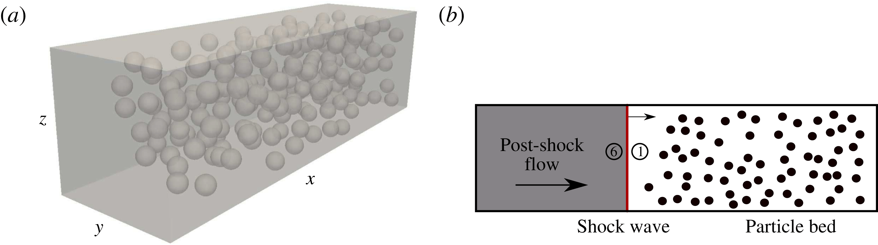
For the numerical simulations we use a finite-volume solver on a body-conforming unstructured grid. A random distribution of monodispersed spheres in a rectangular box, as shown in figure 1(a), is considered. The region of gas flow exterior to the spheres is discretized with a well-resolved unstructured grid. A second-order-accurate AUSM+ (Liou Reference Liou1996) scheme is used for the flux computation and the gradients are modified using a weighted essentially non-oscillatory (WENO) reconstruction technique (Haselbacher Reference Haselbacher2005). Time integration is performed using a third-order Runge–Kutta method. This code has been tested and validated previously for numerous problems involving compressible flows with shock waves. Validation and verification of the numerical scheme can be found in Ling, Haselbacher & Balachandar (Reference Ling, Haselbacher and Balachandar2009), Parmar et al. (Reference Parmar, Haselbacher and Balachandar2009), Ling et al. (Reference Ling, Wagner, Beresh, Kearney and Balachandar2012, Reference Ling, Haselbacher, Balachandar, Najjar and Stewart2013).
During the passage of the shock, the particles are assumed to remain rigid and immobile during the short durations that are considered in this study. The configuration shown in figure 1(a) can thus serve as a good approximation for an incident shock propagating through a porous medium. We also consider this configuration to well approximate incident shock propagation through a random dispersion of spherical particles. The short-lived transient force, created as the shock interacts with the particle, imparts a near impulsive force on the particle. If the particle was allowed to freely move, as shown by Ling et al. (Reference Ling, Haselbacher, Balachandar, Najjar and Stewart2013), the ratio of change in particle velocity due to this impulsive force to that of fluid velocity across the shock scales as the fluid-to-particle density ratio. For example, for an aluminium particle in air, the density ratio is
 $O(1000)$
and the initial impulsive gain in particle velocity is small. The time scale associated with significant particle movement is therefore relatively long due to the large inertia of the particle (fluid-to-particle density ratio is large). Thus, for the situation and time scales considered here, it is reasonable to ignore particle movement.
2.3 Drag
The drag coefficient is defined by
 $$\begin{eqnarray}\boldsymbol{C}_{D}={\displaystyle \frac{\boldsymbol{F}}{{\textstyle \frac{1}{2}}\unicode[STIX]{x1D70C}_{6}u_{6}^{2}A}},\end{eqnarray}$$
where
 $\boldsymbol{F}$
is the force,
 $\unicode[STIX]{x1D70C}_{6}$
the post-incident shock density,
 $u_{6}$
the corresponding post-incident shock velocity, and
 $A$
the cross-section of the particle. Subscript 6 is assigned to the post-incident shock properties and subscript 1 is assigned to the ambient state. Subscripts 2–5 are introduced in § 3 and are assigned to the intermediate states that connect the post-incident shock state with the ambient state. For a sphere,
 $A=\unicode[STIX]{x03C0}d_{p}^{2}/4$
, where
 $d_{p}$
is the particle diameter. Note that since we are carrying out inviscid simulations, only the pressure contributes to the force. The force components are therefore given by
 $$\begin{eqnarray}F_{i}=\boldsymbol{F}\boldsymbol{\cdot }\hat{\boldsymbol{e}}_{i}\equiv \int _{S_{p}}p\,\hat{\boldsymbol{n}}\boldsymbol{\cdot }\hat{\boldsymbol{e}}_{i}\,\text{d}S,\end{eqnarray}$$
where
 $\hat{\boldsymbol{e}}_{i}$
is the unit vector in the
 $x_{i}$
-direction,
 $\hat{\boldsymbol{n}}$
the outward pointing normal, and
 $S_{p}$
the surface of the particle. In this way the drag coefficients in the (
 $x,y,z$
)-directions are given by
 $$\begin{eqnarray}C_{D}={\displaystyle \frac{F_{x}}{{\textstyle \frac{1}{2}}\unicode[STIX]{x1D70C}_{6}u_{6}^{2}A}},\quad C_{D,y}={\displaystyle \frac{F_{y}}{{\textstyle \frac{1}{2}}\unicode[STIX]{x1D70C}_{6}u_{6}^{2}A}},\quad C_{D,z}={\displaystyle \frac{F_{z}}{{\textstyle \frac{1}{2}}\unicode[STIX]{x1D70C}_{6}u_{6}^{2}A}}.\end{eqnarray}$$
The total transverse drag coefficient is given by
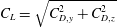 $C_{L}=\sqrt{C_{D,y}^{2}+C_{D,z}^{2}}$
, and the total drag coefficient is given by
 $C_{D,T}=\sqrt{C_{D}^{2}+C_{D,y}^{2}+C_{D,z}^{2}}$
.
2.4 Geometry, simulation set-up, and boundary conditions
In this paper we consider particles placed randomly in a three-dimensional rectangular box; the computational domain and distribution of particles for a fixed volume fraction of 10 % can be seen in figure 1(a). The computational domain has equal
 $y$
and
 $z$
edge lengths, with an extended
 $x$
length that is in the direction of the flow. The computational domain shown in figure 1(a) can be separated into two distinct regions: (i) a shocked air side that is upstream of the incident shock wave (the state in this region is denoted by
 $\unicode[STIX]{x2465}$
), and (ii) a pre-shocked quiescent ambient air into which the incident shock wave is moving (the state in this region is denoted by
 $\unicode[STIX]{x2460}$
). The two regions are marked in figure 1(b).
(a) Diagram of computational domain with 200 rigid particles randomly dispersed. (b) Incident shock wave moving into a bed of particles.

Since we are solving the inviscid equations, there are only a few relevant length scales in the problem. These are the particle diameter, the mean inter-particle distance, and the length scale associated with the unit cell of the particle bed. The mean inter-particle distance is related to global particle volume fraction defined by
 $$\begin{eqnarray}\unicode[STIX]{x1D719}_{1}={\displaystyle \frac{V_{p}N_{p}}{V_{c}}}.\end{eqnarray}$$
All the particles have the same diameter and the volume of a single particle is given by
 $V_{p}=(\unicode[STIX]{x03C0}/6)d_{p}^{3}$
. Here,
 $N_{p}$
is the total number of particles within the computational domain and
 $V_{c}$
is the volume of the unit cell that contains the
 $N_{p}$
particles. The domain is chosen to be 8 particle diameters in length along the
 $y$
and
 $z$
directions. Along the streamwise direction the computational domain is separated into an upstream region without particles and a downstream region containing a random distribution of particles. The streamwise length of the computational domain containing the particles is chosen to be approximately 12 particle diameters, with the precise value chosen such that as the particle volume fraction varied from 10 % to 25 %; the number of particles within the computational domain varied from 200 to 500, respectively. Particles are randomly placed following a process known as the random sequential addition process (Torquato Reference Torquato2002), where each new particle’s location is randomly chosen within the downstream section of the computational domain with the following two constraints: (i) a minimum allowable inter-particle spacing is maintained at
 $d_{p}/20$
, and (ii) a minimum allowable spacing between a particle and the domain walls along the
 $y$
and
 $z$
directions is also maintained at
 $d_{p}/20$
.
The pre-shock state is quiescent ambient air with
 $p_{1}=101.325$
kPa and
 $\unicode[STIX]{x1D70C}_{1}$
 $=1.2048~\text{kg}~\text{m}^{-3}$
. The post-shock conditions for a moving air shock Mach number of
 $M_{s}=3.0$
, as determined by the Rankine–Hugoniot relations for an ideal gas with
 $\unicode[STIX]{x1D6FE}=1.4$
and
 $R=287.04~\text{J}~\text{kg}^{-1}~\text{K}^{-1}$
, are
 $p_{6}=1047.025$
kPa,
 $T_{6}=784.951$
K,
 $\unicode[STIX]{x1D70C}_{6}=4.647~\text{kg}~\text{m}^{-3}$
, and
 $u_{6}=762.529~\text{m}~\text{s}^{-1}$
. The post-shock Mach number is
 $M_{6}=1.36$
. The shock speed in the absence of particles is
 $u_{s}=1029.678~\text{m}~\text{s}^{-1}$
. Note that the post-shock pressure
 $p_{6}$
in air remains well below the yield strength for most materials (0.2 GPa), and so we do not expect the particles to deform.
For each volume fraction the simulation domain length in the streamwise
 $x$
-direction is chosen large enough to avoid disturbances/reflections from upstream and downstream boundaries. The upstream boundary is treated as a constant inflow boundary with inflow at post-incident shock properties, while all other boundaries, including the particle surfaces, are treated as slip walls.
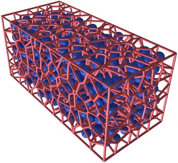
Voronoi tessellation of the domain with 500 randomly placed particles;
 $\unicode[STIX]{x1D719}_{1}=25\,\%$
.

2.5 Data analysis
We characterize the randomized particle bed by generating a three-dimensional Voronoi tessellation of the domain, where the centres of the Voronoi cells are the centres of the particles in the computational domain. Voro++ (Rycroft Reference Rycroft2009) is used to compute the Voronoi tessellation. Figure 2 shows a sample Voronoi tessellation of a random particle bed for a 25 % volume fraction bed. The orange lines in figure 2 mark the boundaries of the Voronoi cells. The blue objects are the particles in the domain. Thus, each particle is associated with a Voronoi cell and the number of Voronoi cell faces corresponds to the number of closest neighbours. By definition, all points within the Voronoi cell are closer to the corresponding particle than all the neighbours. The size of the Voronoi cell around each particle is the measure of the local volume associated with each particle. This local volume fraction was computed for each particle in every simulation. The equation used to calculate the local volume fraction of the
 $i$
th particle is given by
 $$\begin{eqnarray}\unicode[STIX]{x1D719}_{1,i}=\frac{V_{p}}{V_{V,i}},\end{eqnarray}$$
where
 $V_{V,i}$
is the Voronoi volume associated with the
 $i$
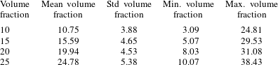
th particle. Each simulation for a different volume fraction has a unique distribution of particles. Even for the same volume fraction, different realizations with different distributions of particles can be considered. The distribution of particles within the computational domain will result in a unique distribution of local volume fractions associated with the particles. The mean, standard deviation, minimum and maximum values of the local volume fraction based on Voronoi volumes for the different simulations are tabulated to provide additional characterization of the different particle distributions. These values are provided in table 1. By definition
 $\sum _{i=1}^{N_{p}}V_{V,i}=V_{c}$
, and as a result it can be seen that the mean local volume fraction based on Voronoi cells will not be precisely equal to
 $\unicode[STIX]{x1D719}_{1}$
. As can be seen from the table, the difference between the two definitions of mean volume fraction is small, but non-zero. At
 $\unicode[STIX]{x1D719}_{1}=10\,\%$
the standard deviation is approximately 36 % of the mean volume fraction, and with increasing volume fraction the standard deviation decreases to approximately 22 % of the mean at
 $\unicode[STIX]{x1D719}_{1}=25\,\%$
. This reduction is consistent with the fact that with increasing volume fraction there is less freedom in the relative position of the neighbouring particles. Observe that for
 $\unicode[STIX]{x1D719}_{1}$
the volume of the smallest Voronoi cell is only 30 % of the mean and the largest Voronoi cell is 250 % of the mean, indicating large variations in the local volume fraction, even though the particles are randomly distributed with uniform probability. The level of variation decreases with increasing
 $\unicode[STIX]{x1D719}_{1}$
, but remains substantially large even at
 $\unicode[STIX]{x1D719}_{1}=25\,\%$
. Another way to quantify this local volume fraction variation is given by
 $$\begin{eqnarray}\unicode[STIX]{x1D719}_{flu_{i}}=\frac{\unicode[STIX]{x1D719}_{1,i}-\unicode[STIX]{x1D719}_{1}}{\unicode[STIX]{x1D719}_{1}},\end{eqnarray}$$
which is just the relative difference between the local volume fraction of the Voronoi cell and the packing fraction.
Statistics of the Voronoi cell volume fractions for different volume fraction grids. The columns correspond to volume fraction
 $\unicode[STIX]{x1D719}_{1}$
as defined by (2.8); the mean volume fraction as determined from Voronoi tessellation; the standard deviation; and the minimum and maximum volume fractions based on (2.9). Note that all quantities are in percentages.

2.6 Grid resolution
Unstructured tetrahedral grids are used for carrying out the fully resolved three-dimensional simulations of an incident shock propagating over a random bed of particles. DistMesh (Persson & Strang Reference Persson and Strang2004) is used to generate the mesh on the surface of the spherical particles. Once a surface mesh is created around the particles, TetGen (Si Reference Si2015) is used to generate the body-conforming unstructured tetrahedral mesh inside the simulation domain. The quality and size of the elements in the domain determines the sharpness of the shock and the accuracy of the solution. Similarly, adequate mesh resolution on the particle surface is required to properly compute aerodynamic forces, which are determined by integrating the pressure on the surface of each particle. The quality and size of the elements are controlled by monitoring the element aspect ratio and maximum element volume. Surface mesh resolution is controlled by specifying the maximum element area.
Previously, a grid resolution study was performed for a face-centred cubic (FCC) array of particles to determine the effect of two constraints – namely, the size of the elements in the domain and the surface mesh resolution per particle – on the solution (Mehta et al.
Reference Mehta, Neal, Jackson, Balachandar and Thakur2016b
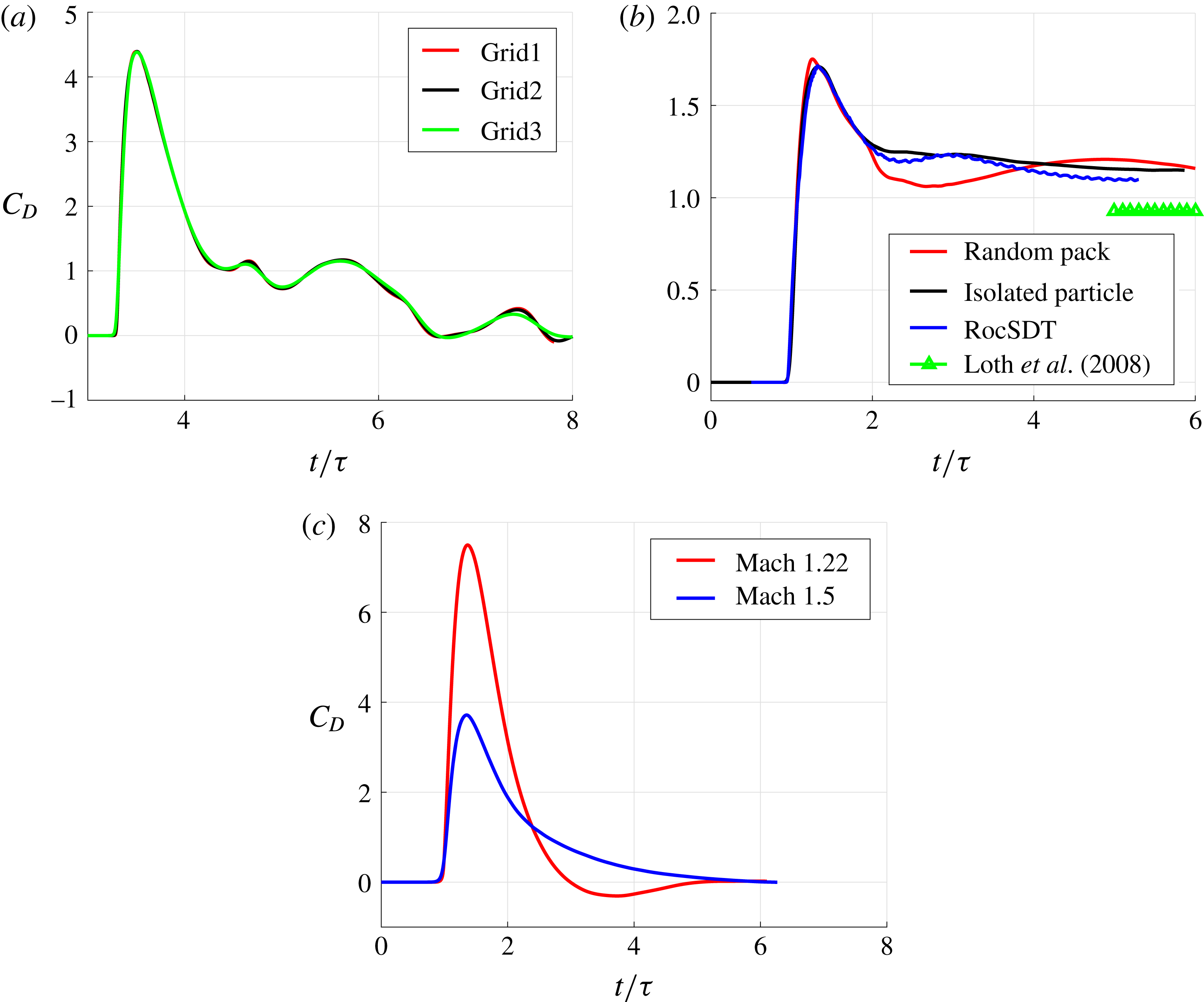
). Twenty-five grids were generated by varying the volume mesh and the surface mesh. Results from three representative simulations are presented in figure 3(a). Here,
 $\unicode[STIX]{x1D70F}$
is the shock–particle interaction time defined by
 $$\begin{eqnarray}\unicode[STIX]{x1D70F}=d_{p}/u_{s},\end{eqnarray}$$
where
 $u_{s}$
is the incident shock speed and
 $d_{p}$
is the particle diameter. For each mesh, the drag coefficient was sampled at a few time instances and compared to that of a well-resolved simulation. In this way the error as a function of resolution was quantified. Based on the results, an optimum grid resolution (mesh size) was selected which provided the best compromise between the numerical error and the computational cost. We then generated unstructured grids for volume fractions of 10, 15, 20 and 25 %. The total cell count for the grids and the number of particles in the random bed as a function of volume fraction are shown in table 2.
Plot of streamwise drag,
 $C_{D}$
, as a function of non-dimensional time,
 $t/\unicode[STIX]{x1D70F}$
, for (a) three grids from a previous grid resolution study (Mehta et al.
Reference Mehta, Neal, Jackson, Balachandar and Thakur2016b
), Grid1 (30 million total elements, 110 000 surface mesh), Grid2 (18 million total elements, 70 000 surface mesh), and Grid3 (6 million total elements, 43 000 surface mesh), here
 $M_{s}=1.5$
and
 $\unicode[STIX]{x1D719}_{1}=10\,\%$
; (b) isolated particle (black), the leading particle in the random pack (red), results from previously published data using RocSDT (Mehta et al.
Reference Mehta, Jackson, Zhang and Balachandar2016a
) (blue), and steady state drag predicted using curve fit presented by Loth (Reference Loth2008) (green), here
 $M_{s}=3.0$
; (c) isolated particle at
 $M_{s}=1.22$
(red) and
 $M_{s}=1.5$
(blue).

Tetrahedral cell counts and number of particles for different volume fractions.

To determine the adequacy of the grid used in these simulations, we show in figure 3(b) a plot of the drag coefficient as a function of non-dimensional time
 $t/\unicode[STIX]{x1D70F}$
for a single isolated particle (black) with that of the first particle in the random bed (red). The metrics that can be compared between the two simulations are the initial rise of the drag coefficient, the peak value of the drag coefficient, and the initial decay of the drag coefficient as the transmitted shock passes over the particle. From the figure we note that (i) both the initial rise and the initial decay in the drag coefficient compare well with that of the single particle; (ii) there is a small deviation of approximately 2 % in the value of the peak drag coefficient; and (iii) that the time that the peak occurs is slightly shifted from that of the single-particle result. The time shift in the peak and the difference in peak values are due to the reduced mesh resolution of each particle compared to the resolution used for the isolated particle. This reduction was necessary to keep the simulation at a reasonable size and cost. Also from the figure we see that for
 $t/\unicode[STIX]{x1D70F}>2$
the drag coefficient of the leading particle deviates from the drag coefficient of the isolated particle. This is because the force history of a particle at later times is influenced by the presence of neighbouring particles. It is evident from the black curve in figure 3(b) that a single isolated particle experiences a constant non-zero drag force at later times. This drag force is the result of a bow shock that forms in front of the spherical particle because of the supersonic post-incident shock flow. The value of this steady state drag force has been previously compared against experimental and numerical fits (Mehta et al.
Reference Mehta, Neal, Jackson, Balachandar and Thakur2016b
). In the same figure, the result from a different numerical code (RocSDT) (Mehta et al.
Reference Mehta, Jackson, Zhang and Balachandar2016a
), but for the same conditions, is also plotted. We can see that the results from these two different codes are in good agreement. The steady state drag force predicted using the curve fit of Loth (Reference Loth2008) is also plotted as symbols. The steady state drag for the black and blue curves gradually approaches the asymptotic limit given by the curve fit of Loth (Reference Loth2008).
Another important factor to consider while analysing the numerical error is the effect of artificial viscosity. The numerical method described in § 2.2 uses the AUSM+ scheme (Liou Reference Liou1996) for shock capturing. We believe that the impact of the associated numerical dissipation on our force results is quite small. To demonstrate this, we plot the non-dimensional drag force on a single isolated particle for incident shock Mach numbers
 $M_{s}=1.22$
and 1.50 in figure 3(c). The post-incident shock Mach numbers are subsonic and their values are 0.31 and 0.60, respectively. Since the post-incident shock flow is inviscid and subsonic, the steady state drag force is zero, as seen in the figure. If the impact of numerical dissipation was significant, then the steady state drag force would have been non-zero for these two simulations. The vorticity magnitude for a Mach 3.0 incident shock interacting with a single isolated spherical particle was monitored over a period of time and was found to be negligible (and therefore not shown here), further indicating that the influence of numerical dissipation is quite small in the present simulation.
3 Riemann solution
Before we proceed to numerical simulations of a planar incident shock propagating through a random bed of particles, in this section we consider shock evolution in a one-dimensional duct with a sudden area reduction. We take the shock to be same as the incident shock of the numerical simulations and to be initially located at the area reduction, where the area changes from 1 to
 $1-\unicode[STIX]{x1D719}_{1}$
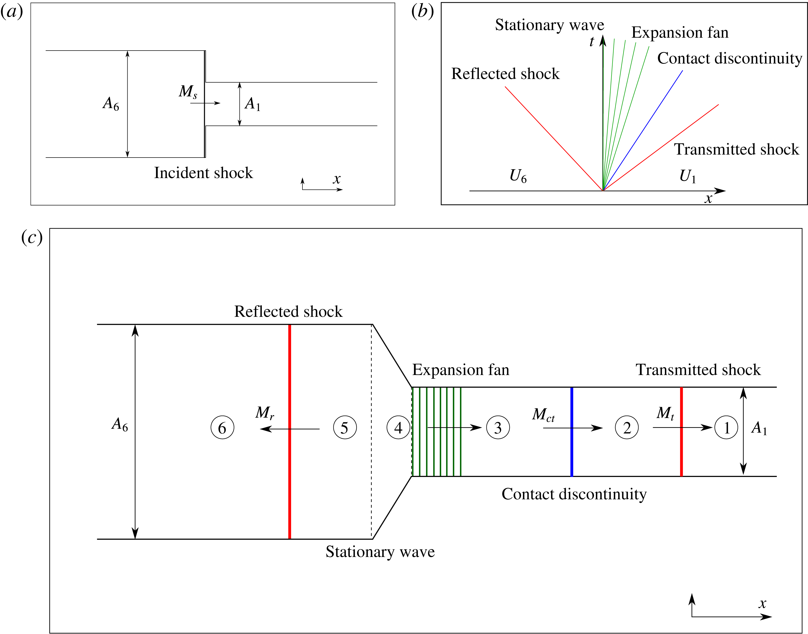
. The subsequent evolution of the flow in this Riemann problem can then be compared with the numerical simulations. As will be discussed below, the Riemann solution allows us to clearly identify four waves (two shocks, one expansion fan, and one contact discontinuity) within the flow and their dependence on area reduction (or particle volume fraction). Due to the chaotic nature of the flow, identification of these waves from the numerical simulations is difficult without the guidance of the Riemann solution. We will quantify the strength of the transmitted shock, reflected shock, and the contact discontinuity as obtained from the Riemann solution, and compare them with those obtained from the numerical simulations in order to assess the effect of shock diffraction and the dissipative role of the shocklets. Similarly, the presence of a resonant expansion fan will be revealed by the Riemann solution, which can be compared with the pressure drop that is observed in the numerical simulations. The instant when the incident shock is positioned exactly at the location of area reduction is shown in figure 4(a), with the pre-shock ambient state on the right marked by
 $\unicode[STIX]{x2460}$
and the post-incident shock high-pressure state on the left marked by
 $\unicode[STIX]{x2465}$
. The left and the right states are related through the Rankine–Hugoniot relations for the incident shock of Mach number
 $M_{s}$
. Figure 4(b) then represents a Riemann problem, where across an imaginary diaphragm located at
 $x=0$
we have the classic problem of a jump in the flow state represented by velocity, pressure and density, but in addition we also have a jump in the cross-sectional area. The solution to this Riemann problem can be obtained by solving (2.1)–(2.3), along with the following equation for the volume fraction evolution
 $$\begin{eqnarray}\frac{\unicode[STIX]{x2202}\unicode[STIX]{x1D719}}{\unicode[STIX]{x2202}t}=0,\end{eqnarray}$$
which simply states that the initial area change remains unchanged over time.
Plot of (a) one-dimensional set-up of incident shock propagation over discontinuous area change, (b) wave configuration based on initial data and (c) approximate locations of waves in the domain.

The above Riemann problem represented by figure 4(a) has been investigated by Lefloch & Thanh (Reference Lefloch and Thanh2003), Kröner & Thanh (Reference Kröner and Thanh2005) and Han et al. (Reference Han, Hantke and Warnecke2012). These investigations are more general than the particular case of an incident shock propagating through a duct of sudden area reduction, as they presented solutions for any combination of values for gas velocity, pressure, density and change in cross-sectional area across the diaphragm. In particular, Han et al. (Reference Han, Hantke and Warnecke2012) classified the general solution into six basic cases for the left-to-middle (L–M) waves and a matching six basic cases for the right-to-middle (R–M) waves, which taken together covers all solutions for all possible initial conditions. The six L–M cases are differentiated according to (i) whether the flow in state
 $\unicode[STIX]{x2465}$
is supersonic or subsonic, and (ii) the ordering of two different areas
 $A_{s}$
and
 $A_{T}$
(defined below) with respect to
 $A_{6}$
and
 $A_{1}$
. The six R–M cases on the right are differentiated similarly. In the absence of resonance there are four waves: a stationary wave with three other elementary waves that can be a shock wave, expansion fan, or a contact discontinuity. For some initial conditions the solution exhibits resonance, which results in a complex resonant wave with two other elementary waves.
Here we apply this general theory for the present case of the post-incident shock state
 $\unicode[STIX]{x2465}$
on one side and pre-shock ambient state
 $\unicode[STIX]{x2460}$
on the other side of the sudden area reduction, as shown in figure 4(a). Let the gas velocity, pressure, density and speed of sound in the left state be
 $u_{6}$
,
 $p_{6}$
,
 $\unicode[STIX]{x1D70C}_{6}$
and
 $c_{6}$
, respectively. The corresponding values on the right are
 $u_{1}$
,
 $p_{1}$
,
 $\unicode[STIX]{x1D70C}_{1}$
and
 $c_{1}$
. Non-dimensional values for our problem for a Mach 3.0 incident shock wave moving into quiescent ambient are given in table 3. For this case the post-incident shock flow on the left is supersonic, therefore
 $u_{6}-c_{6}>0$
and also
 $u_{1}+c_{1}\geqslant 0$
. Furthermore, the particle bed represents an area reduction (i.e.,
 $A_{6}>A_{1}$
). Following Han et al. (Reference Han, Hantke and Warnecke2012), two more area parameters
 $A_{T}$
and
 $A_{S}$
are defined as
 $$\begin{eqnarray}\displaystyle & \displaystyle A_{T}=A_{1}\left|\frac{u_{6}}{c_{6}}\right|\left[\left(\frac{\unicode[STIX]{x1D6FE}-1}{\unicode[STIX]{x1D6FE}+1}\right)\left(\frac{u_{6}}{c_{6}}\right)^{2}+\left(1-\frac{\unicode[STIX]{x1D6FE}-1}{\unicode[STIX]{x1D6FE}+1}\right)\right]^{-(1/(2((\unicode[STIX]{x1D6FE}-1)/(\unicode[STIX]{x1D6FE}+1))))}, & \displaystyle\end{eqnarray}$$
 $$\begin{eqnarray}\displaystyle & \displaystyle A_{S}=A_{1}\left|\frac{{u_{6}}^{0}}{{c_{6}}^{0}}\right|\left[\left(\frac{\unicode[STIX]{x1D6FE}-1}{\unicode[STIX]{x1D6FE}+1}\right)\left(\frac{{u_{6}}^{0}}{{c_{6}}^{0}}\right)^{2}+\left(1-\frac{\unicode[STIX]{x1D6FE}-1}{\unicode[STIX]{x1D6FE}+1}\right)\right]^{-(1/(2((\unicode[STIX]{x1D6FE}-1)/(\unicode[STIX]{x1D6FE}+1))))}, & \displaystyle\end{eqnarray}$$
where
 ${u_{6}}^{0}$
and
 ${c_{6}}^{0}$
are given by
 $$\begin{eqnarray}\displaystyle & \displaystyle {u_{6}}^{0}=\left(\frac{\unicode[STIX]{x1D6FE}-1}{\unicode[STIX]{x1D6FE}+1}\right)u_{6}+\left(1-\frac{\unicode[STIX]{x1D6FE}-1}{\unicode[STIX]{x1D6FE}+1}\right)\frac{(c_{6})^{2}}{u_{6}}, & \displaystyle\end{eqnarray}$$
 $$\begin{eqnarray}\displaystyle ({c_{6}}^{0})^{2} & = & \displaystyle (c_{6}^{2})\left[\left(1+\frac{\unicode[STIX]{x1D6FE}-1}{\unicode[STIX]{x1D6FE}+1}\right)\left(\frac{u_{6}}{c_{6}}\right)-\left(\frac{\unicode[STIX]{x1D6FE}-1}{\unicode[STIX]{x1D6FE}+1}\right)\left(\frac{c_{6}}{u_{6}}\right)\right]\nonumber\\ \displaystyle & & \displaystyle \times \left[\left(\frac{\unicode[STIX]{x1D6FE}-1}{\unicode[STIX]{x1D6FE}+1}\right)\left(\frac{u_{6}}{c_{6}}\right)+\left(1-\frac{\unicode[STIX]{x1D6FE}-1}{\unicode[STIX]{x1D6FE}+1}\right)\left(\frac{c_{6}}{u_{6}}\right)\right].\end{eqnarray}$$
For our initial conditions, the values of
 $A_{T}$
and
 $A_{S}$
are computed, and we note that
 $A_{6}>A_{S}>A_{T}>A_{1}$
. Based on this ordering, we classify the L–M wave structure as belonging to case VI and correspondingly the R–M wave structure as belonging to case II, according to the classification of Han et al. (Reference Han, Hantke and Warnecke2012). The resulting resonant wave structure that is most relevant for our set-up is given in figure 4(b). Immediately following the arrival of the incident shock at the sudden area reduction, there is a reflected shock moving to the left, a stationary wave at
 $x=0$
across which area reduces, followed by a resonant expansion fan whose head is attached to the stationary wave while its tail moves to the right, followed by a contact discontinuity that also travels to the right, and finally a rightward moving transmitted shock. Similar wave structure has been previously discussed by Regele et al. (Reference Regele, Rabinovitch, Colonius and Blanquart2014).
Non-dimensional flow properties across the domain for 10 % area reduction and for an incident shock Mach number of 3. Here,
 $p_{6}=1047.025$
kPa,
 $\unicode[STIX]{x1D70C}_{6}=4.647~\text{kg}~\text{m}^{-3}$
and
 $u_{6}=762.529~\text{m}~\text{s}^{-1}$
.

The wave structure described in figure 4(b) is illustrated with approximate relative positions of different wave components in a duct with sudden area reduction in figure 4(c). State
 $\unicode[STIX]{x2465}$
represents the post-incident shock flow ahead of the reflected shock moving to the right and the Mach number of the reflected shock will be denoted by
 $M_{r}$
. State
 $\unicode[STIX]{x2464}$
represents the subsonic side of the reflected shock, and the fluid continues to travel in the positive streamwise direction. Between states
 $\unicode[STIX]{x2464}$
and
 $\unicode[STIX]{x2463}$
there is a sudden area change where the incoming subsonic flow expands isentropically, and this is the stationary wave mentioned previously. At state
 $\unicode[STIX]{x2463}$
there is a resonant expansion wave that is coincident with the stationary wave. The upstream front of the expansion fan is stationary, while the downstream front is moving into a region whose state is given by
 $\unicode[STIX]{x2462}$
. States
 $\unicode[STIX]{x2462}$
and
 $\unicode[STIX]{x2461}$
are connected by a contact discontinuity across which the density and temperature change. The ambient state
 $\unicode[STIX]{x2460}$
and state
 $\unicode[STIX]{x2461}$
are connected by the transmitted shock, which is travelling in the positive streamwise direction and whose Mach number is denoted by
 $M_{t}$
.
We now describe the step-by-step process involved in obtaining the unique solution represented by the wave structure given in figure 4(c). We consider a representative example with incident shock Mach number 3.0 and an area change of 10 % across the particle bed.
Step 1: We are given the post-incident shock state
 $\unicode[STIX]{x2465}$
, from which for varying values of the reflected shock Mach number
 $M_{r}$
we obtain the reflected shock speed and the flow quantities across it for state
 $\unicode[STIX]{x2464}$
. We now demand that (i) the velocity of the reflected shock
 $u_{r}$
be negative; i.e., that the reflected shock must move upstream, and (ii) the gas velocity of state
 $\unicode[STIX]{x2464}$
be positive. These constraints restrict the possible reflected shock Mach numbers to be between 1.3580 and 2.1040. For these possible values of the reflected shock Mach number, the flow for state
 $\unicode[STIX]{x2464}$
is always subsonic.
Step 2: The next step is to match the post-reflected-shock state
 $\unicode[STIX]{x2464}$
with the stationary wave, which is isentropic flow through an area change, to obtain the flow state
 $\unicode[STIX]{x2463}$
. In our case the area change is like a contracting nozzle, since
 $(A_{6}=A_{5})>(A_{4}=A_{1})$
. A subsonic inflow into a contracting nozzle can at most reach a sonic state. In the present work we consider area reductions of 10 % to 25 %, and in all these cases the flow becomes sonic for state
 $\unicode[STIX]{x2463}$
. This is indeed a condition for resonance, since only then will the head of the expansion fan that is to follow, whose velocity with respect to the local flow must be sonic, remain stationary in the laboratory frame, and coincide with the stationary wave. For smaller area reductions it is possible that the flow at state
 $\unicode[STIX]{x2463}$
may still be subsonic and deviate from the scenario shown in figure 4(c). However, if the flow reaches a sonic state after the area reduction, there is only one unique possible solution for the reflected shock and the post-reflected-shock flow. For example, for an area change of 10 %, the flow must enter the area reduction at a Mach number of 0.6787 to reach the sonic condition (or Mach 1.0) as it exits the area reduction. The corresponding reflected shock Mach number is 1.4180, with a slow upstream velocity of
 $u_{r}/u_{6}=-0.044$
. Table 3 summarizes the flow properties for states
 $\unicode[STIX]{x2464}$
and
 $\unicode[STIX]{x2463}$
.
Step 3: The resonant wave is an expansion fan whose upstream front is stationary and the downstream front is moving at the local speed of sound into a region with state
 $\unicode[STIX]{x2462}$
. The expansion fan is an isentropic process and flow properties within the expansion fan can be easily evaluated in terms of the Mach number corresponding to state
 $\unicode[STIX]{x2462}$
. In particular, we calculate the gas velocity and pressure for state
 $\unicode[STIX]{x2462}$
for varying values of
 $M_{3}$
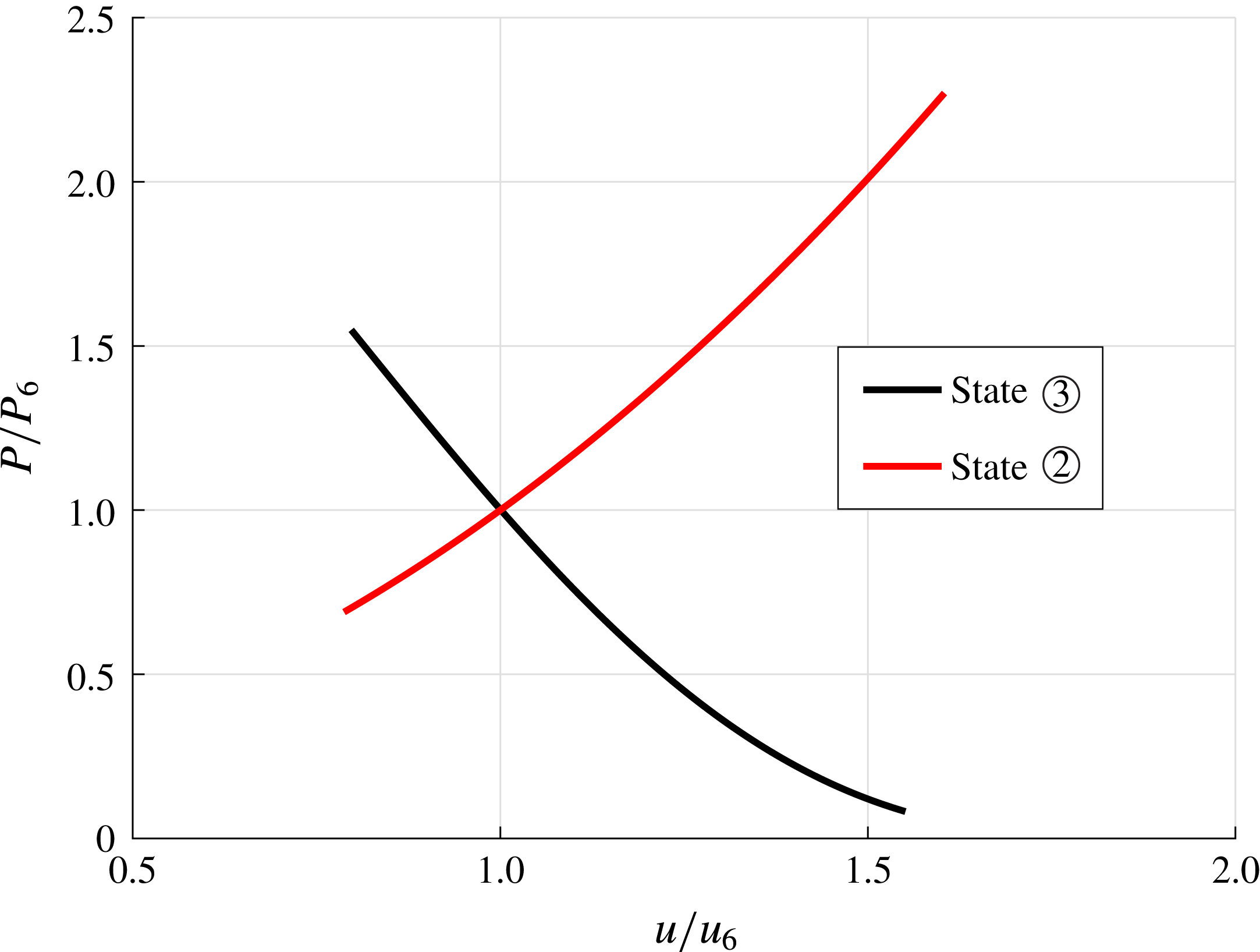
and plot them in figure 5 as the black curve.
Step 4: We know that the flow with state
 $\unicode[STIX]{x2462}$
is followed by a contact discontinuity to state
 $\unicode[STIX]{x2461}$
and a transmitted shock from state
 $\unicode[STIX]{x2461}$
to
 $\unicode[STIX]{x2460}$
. Since the pressure and velocity do not change across a contact discontinuity, the pressure and velocity behind the transmitted shock for state
 $\unicode[STIX]{x2461}$
must match those presented in figure 5 for state
 $\unicode[STIX]{x2462}$
. Since the ambient conditions at
 $\unicode[STIX]{x2460}$
are known, the state of the gas behind the transmitted shock can be fully expressed in terms of the transmitted shock Mach number,
 $M_{t}$
. We vary the transmitted shock number and plot in figure 5 the resulting pressure versus velocity for state
 $\unicode[STIX]{x2461}$
as the red curve. It is clear from the plots that there is a unique solution given by the intersection point between the two curves, which yields a common pressure and velocity for states
 $\unicode[STIX]{x2462}$
and
 $\unicode[STIX]{x2461}$
. We find the transmitted shock Mach number to be nearly the same as that of the incident shock (i.e.,
 $M_{t}\approx 3$
), with a non-dimensional velocity of
 $u_{t}/u_{6}=1.3499$
.
Step 5: The corresponding densities for states
 $\unicode[STIX]{x2462}$
and
 $\unicode[STIX]{x2461}$
, however, are not equal. This results in a contact discontinuity across which both density and temperature change. The contact discontinuity travels downstream at the local gas velocity. In the case of 10 % volume reduction the density jump across the contact discontinuity is 1.0137. Table 3 summarizes the flow properties for states
 $\unicode[STIX]{x2462}$
and
 $\unicode[STIX]{x2461}$
. The strength of the contact discontinuity is computed by taking the ratio of densities in states
 $\unicode[STIX]{x2462}$
and
 $\unicode[STIX]{x2461}$
, which is presented in table 3.
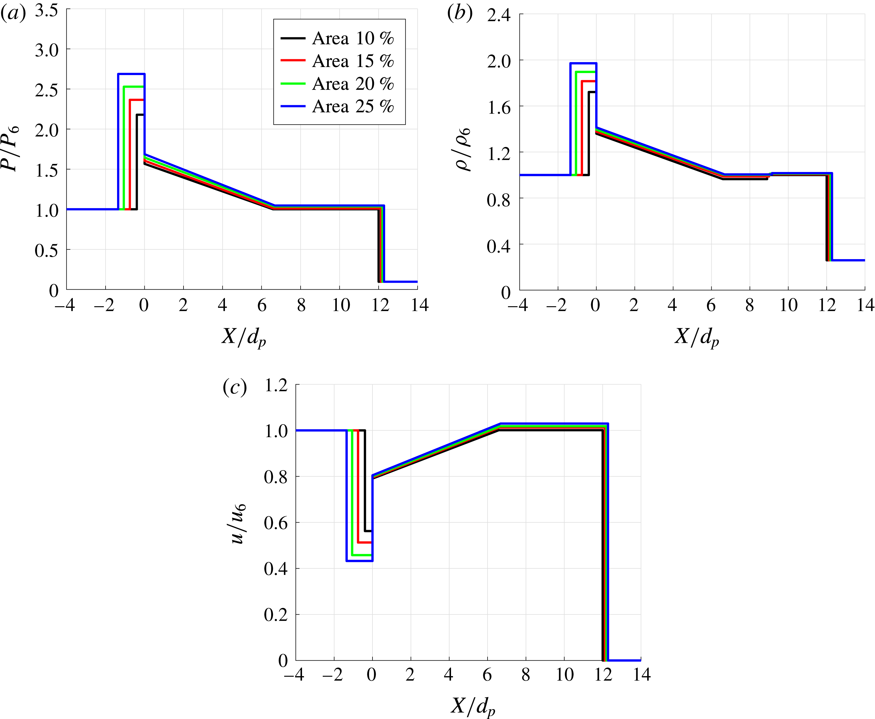
We repeat Steps 1–5 for different area changes to obtain the flow properties across the wave structure. Plots of non-dimensional pressure, density and velocity for different area changes are presented in figure 6. In addition, the key properties of these solutions are listed in table 4. These baseline Riemann solutions of the sudden contraction will be used to compare with those from the numerical simulations of incident shock propagation through a random particle bed to be presented in the subsequent sections.
Plot of non-dimensional pressure,
 $P/P_{6}$
, against non-dimensional velocity,
 $u/u_{6}$
, for varying transmitted shock Mach numbers for states
 $\unicode[STIX]{x2462}$
and
 $\unicode[STIX]{x2461}$
.

Plot of non-dimensionalized (a) pressure, (b) density, and (c) velocity across the domain at
 $t/\unicode[STIX]{x1D70F}=12$
for
 $\unicode[STIX]{x1D719}_{1}=10\,\%$
, 15 %, 20 % and 25 %.

Flow properties across the domain for different area reductions and for an incident shock Mach number of 3.

The key observations from the Riemann solution that will be of importance later in interpreting the numerical solution are (i) the reflected shock continues to move upstream at a very slow velocity and will not reach a steady state as in a bow shock, (ii) the transmitted shock is slightly stronger than the incident shock, (iii) the strength of the contact discontinuity is quite weak, and (iv) there is substantial pressure drop immediately downstream of the area change due to the resonant expansion fan, which is not due to any dissipative mechanism.
4 Simulation results
In this section we present numerical results of an incident shock propagating over a random bed of particles that are held fixed in space and time. We study the effect of volume fraction for a fixed incident shock Mach number
 $M_{s}=3$
. We compute the individual force histories on each particle as well as flow field information to extract data about the behaviour of the shock wave as it propagates through the random particle bed. The main insights that can be obtained from the results are an understanding of how the interaction of a shock with the distribution of particles affects its propagation, as well as how the presence of a large number of adjacent particles modifies the force experienced by each individual particle as it interacts with the shock wave.
4.1 Streamwise force on the particles
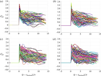
The time histories of streamwise force for an incident shock propagating through a three-dimensional random bed of particles are presented in figure 7 for the four different volume fractions considered in this study. Note that the streamwise force history for each particle is shown in the figure; since each bed contains hundreds of particles, there are hundreds of curves. The time axis has been shifted based on the incident shock arrival time. This makes the force history of all the particles align for each particle on the shifted time axis, even though in reality each particle sees the incident shock at different times based on its streamwise location. The force plots show a chaotic and tangled appearance of the drag force histories. The time-resolved force histories of each particle paint a picture of the flow field that every particle sees during the shock wave interaction and the fluctuations during the post-incident shock flow.
Plot of streamwise drag coefficient,
 $C_{D}$
, as a function of shifted non-dimensional time,
 $(t-t_{arrival})/\unicode[STIX]{x1D70F}$
, and for volume fractions of (a)
 $\unicode[STIX]{x1D719}_{1}=10\,\%$
, (b)
 $\unicode[STIX]{x1D719}_{1}=15\,\%$
, (c)
 $\unicode[STIX]{x1D719}_{1}=20\,\%$
and (d)
 $\unicode[STIX]{x1D719}_{1}=25\,\%$
.

In a sense each time history of force shown in figure 7 qualitatively resembles that shown by the black curve in figure 3(b). This includes the characteristic feature of a rapid rise in the streamwise force due to the incident shock, whose arrival time depends on the streamwise location of the particle. The initial force history for the leading (leftmost) particles in the random bed is identical to that of an isolated particle; i.e., at times before the transverse reflections from the neighbouring particles arrive to disrupt the incident shock, the behaviour of the flow is identical to that of an isolated particle. In the classical single particle shock interaction case, the drag coefficient will quickly rise as the incident shock passes over the particle, and then the drag coefficient will either drop to zero for a subcritical inviscid case or to a constant non-zero value for the supercritical case. For the supercritical case, the post-incident shock velocity is supersonic, and a bow shock forms upstream of the particle, causing the wave drag to be non-zero. Thus, as a result of interaction with the incident shock front, each force history rapidly reaches a peak and decays over time.
However, substantial differences are seen between the different force histories, emphasizing the important role of secondary interactions with the reflected waves and wakes of the other particles in the domain. For example, we can see that there are negative drag coefficients for some of the particles in the bed, indicating that the pressure behind the particle is larger than the pressure in front of it. In comparison, for an isolated particle subjected to a Mach 3 incident shock wave, at all later times the drag coefficient steadily approaches a value close to unity due to the formation of a bow shock ahead of the particle. The presence of large variations in the streamwise force, including negative force values, indicate the strong influence of neighbours on the force history experienced by the different particles. We can clearly observe the effect of volume fraction on the drag force experienced by the particles. As the volume fraction increases, the magnitude of this particle-to-particle variation in the drag force also increases. For higher volume fractions,
 $\unicode[STIX]{x1D719}_{1}=20\,\%$
and 25 %, the magnitude of post-incident shock drag force is comparable to that the of peak drag. There is also substantial variation in the peak drag force experienced by the different particles, which is hard to observe in figure 7. Hence in what follows we will quantify both the mean drag force within the particle bed as well as the particle-to-particle variation in the peak drag force seen within the bed.
Plot of peak streamwise drag coefficient,
 $C_{D,peak}$
, as a function of non-dimensional distance,
 $x/d_{p}$
. The red curve is the least-squares linear fit for the data,
 $\langle C_{D,peak}\rangle$
. Here, (a)
 $\unicode[STIX]{x1D719}_{1}=10\,\%$
, (b)
 $\unicode[STIX]{x1D719}_{1}=15\,\%$
, (c)
 $\unicode[STIX]{x1D719}_{1}=20\,\%$
and (d)
 $\unicode[STIX]{x1D719}_{1}=25\,\%$
.

Least-squares curve fit statistics for peak streamwise drag
 $C_{D,peak}$
.

One way to simplify the characterization of the complex force histories seen in figure 7 is to focus only on the peak values of
 $C_{D}$
for each particle. Figure 8 plots the peak streamwise drag coefficient,
 $C_{D,peak}$
, as a function of non-dimensional streamwise distance
 $x/d_{p}$
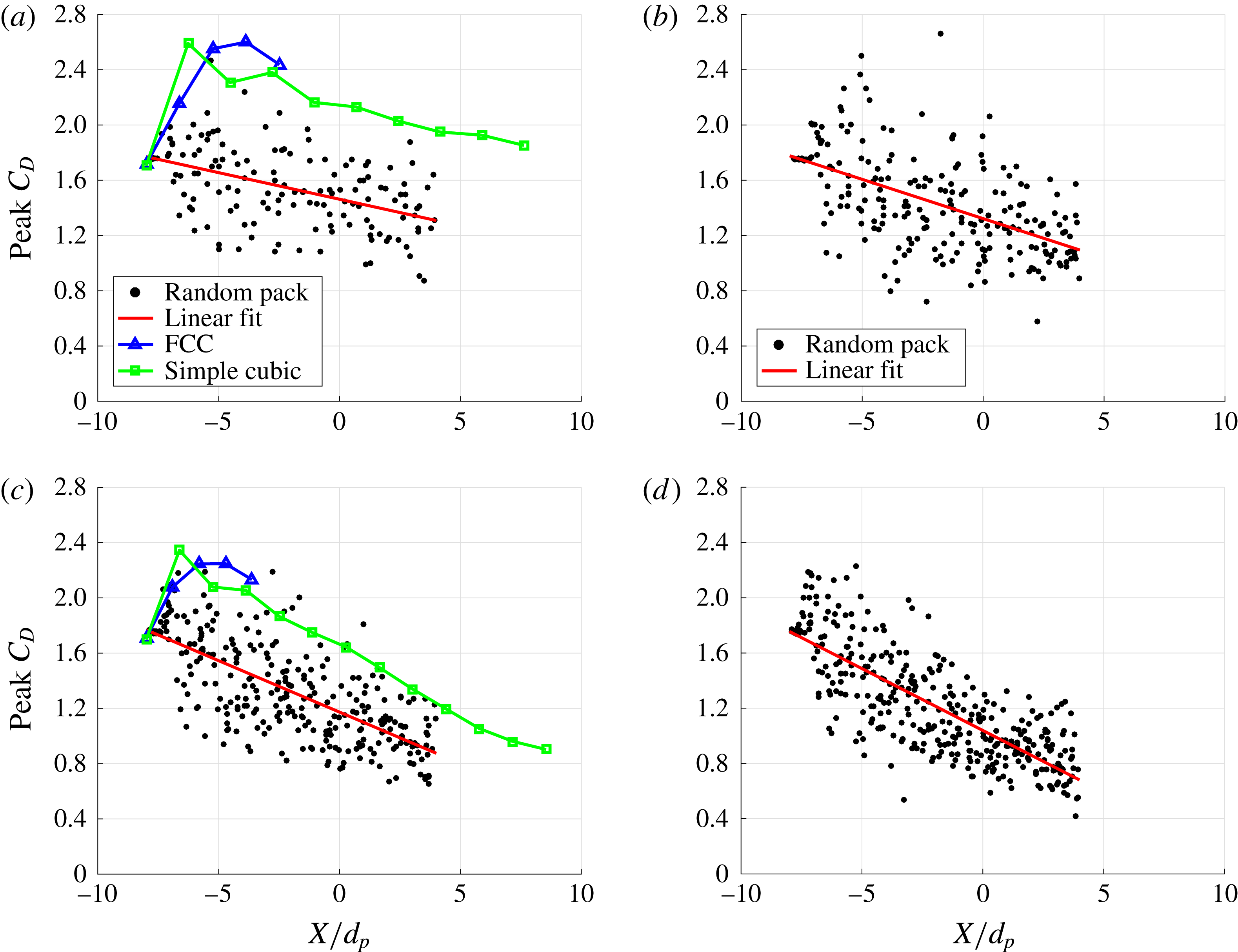
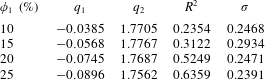
of the particle centre for the same four volume fractions shown in figure 7. It is clear from the figure that there is a downward trend in the peak drag, that there is stochastic variation, and that the rate of decrease in the peak drag increases as the volume fraction increases. For each volume fraction, a least-squares linear fit for the peak drag is carried out. The linear fit is plotted as the red line in the figure, and is given by
 $\langle C_{D,peak}\rangle =q_{1}\unicode[STIX]{x1D709}/d_{p}+q_{2}$
, where
 $\unicode[STIX]{x1D709}$
is measured from the leading edge of the particle bed. Here
 $q_{1}$
is the slope of the line and can be thought of as the rate of decrease of peak drag, and
 $q_{2}$
is the intercept at
 $\unicode[STIX]{x1D709}/d_{p}=0$
, or the mean peak drag experienced by the leading particles. For the four different volume fractions, table 5 presents
 $q_{1}$
and
 $q_{2}$
along with the goodness of the fit measured in terms of the
 $R^{2}$
value and also the rms value (
 $\unicode[STIX]{x1D70E}$
) of the deviation of the actual peak
 $C_{D}$
about the fit. Since
 $\langle C_{D,peak}\rangle$
is typically in the range 0.8 to 1.6, the value of
 $\unicode[STIX]{x1D70E}$
suggests more than 20 % particle-to-particle variation in the peak drag coefficient.
For comparison, also plotted in figure 8(a,c) are the peak drag coefficients obtained in the case of Mach 3 incident shock propagation over a FCC array of particles at 10 % and 20 % volume fractions. The figure clarifies the importance of particle arrangement. The results for the FCC arrangement are for five streamwise planes of particles (Mehta et al. Reference Mehta, Neal, Jackson, Balachandar and Thakur2016b ), which are shown in the figure. By symmetry, all particles within a streamwise plane of FCC array experience the same streamwise drag force. For both volume fractions the drag coefficient of the FCC arrangement increased from the leading (first) plane of particles to the third plane, and then slightly decreased towards the fifth plane of particles. Three mechanisms were identified contributing to the downstream variation of peak drag force. (i) As the incident shock transmits through the particle bed, diffraction around each plane of particles can lead to regions of shock focusing in the wake and contribute to higher drag on the subsequent plane of particles. (ii) If the Mach number of the post-incident shock flow is greater than the critical value, shocklets form around the particles, which dissipate energy from the transmitted shock as it propagates into the bed. This dissipation contributes to the downstream weakening of the transmitted shock, and hence reduction in the peak drag force. (iii) Further wave reflections from the neighbouring particles contribute constructive and destructive interferences and corresponding modifications of the force. In the case of the FCC arrangement, shock focusing effect dominates over the first few planes of particles. In the random array, the effect of shock focusing and constructive interference can be seen as the cause of the above-average peak force experienced by some of the particles. However, since the particles are randomly distributed, some particles locally experience destructive interference, causing a reduction in the peak drag force. When averaged over all the particles at any streamwise location, we see that the combined effect of these two opposing effects is to decrease the mean peak drag force as compared to the peak drag force of a structured array, where for the present volume fractions the effect of interference for each particle is always constructive. This effect highlights the impact of random distribution on the average drag force experienced by the particles. For both the random pack and the structured array, the effect of dissipation is evident from the decreasing peak drag force as the depth of the bed increases, which is approximately the same in both cases.
Also plotted in figure 8(a,c) are the results for simple cubic (SC) array of particles at 10 % and 20 % volume fractions. In this case 10 planes of particles are considered in the streamwise direction and due to symmetry the drag force on all the particles that lie on a streamwise plane are the same. As can be expected, the peak drag force for the leading particle in the random, FCC and simple cubic array are the same. The peak drag force on the subsequent planes of the SC arrangement are qualitatively similar to that of the FCC arrangement. In the case of the SC arrangement, the peak drag increases from the first to the second plane, but steadily decreases from the third plane onwards. It is interesting to observe that the peak drag force in the structured arrays are substantially higher than the mean drag of the random array, thus emphasizing the importance of the arrangement on promoting constructive interference. The streamwise decay of the peak drag force in the SC arrangement is approximately the same as that for the random array, signifying similarities in their shocklet-induced dissipation.
In figure 8(a,c) it is seen that the peak drag force for the structured arrays is substantially higher than the mean drag force for the random pack. We note that this behaviour will not be always true. Depending on the incident shock Mach number and the inter-particle spacing, the particles behind the leading particle in a structured array an have a lower peak drag force (due to destructive interference) compared to the peak drag force of the leading particle. This was investigated by Sridharan et al. (Reference Sridharan, Jackson, Zhang and Balachandar2015).
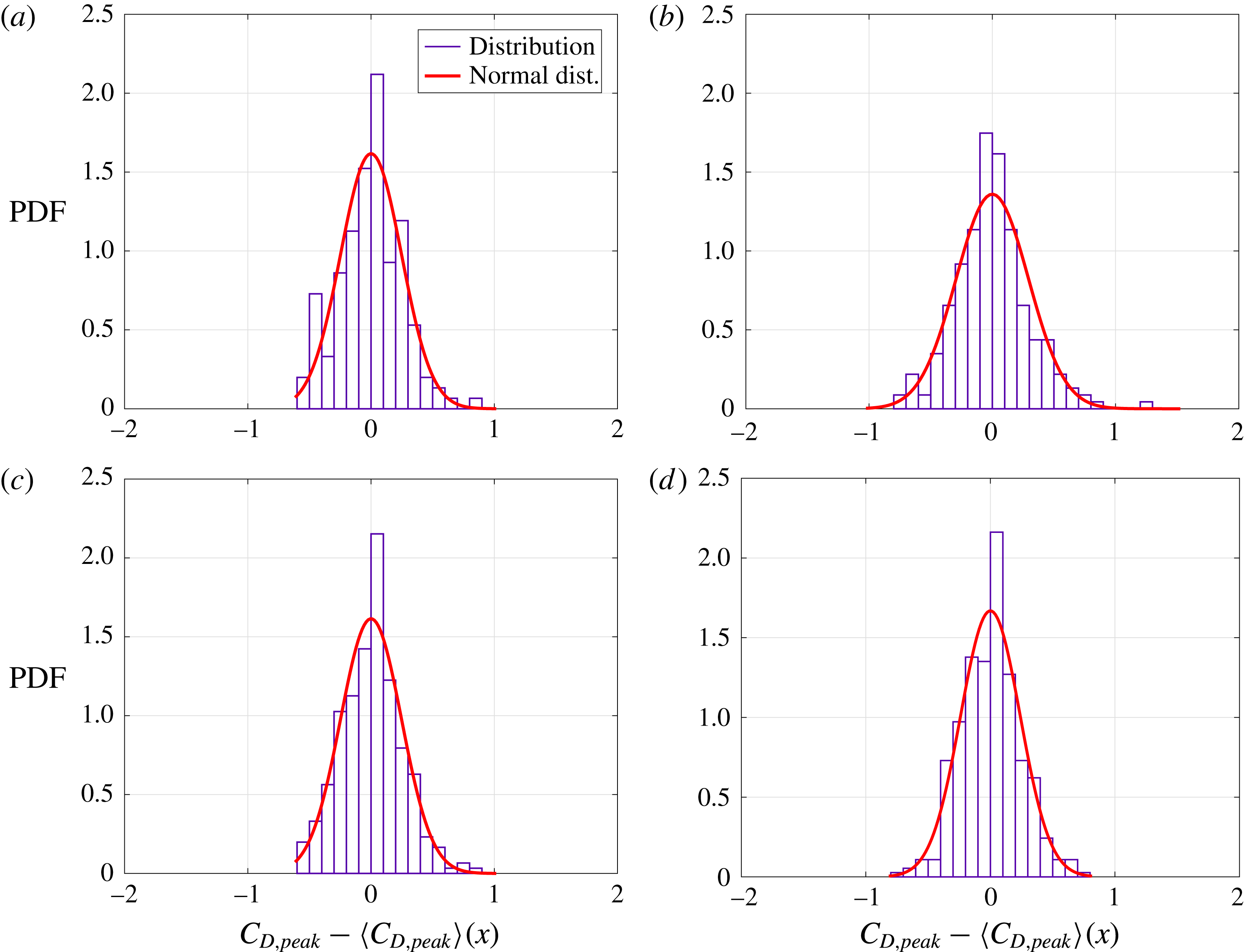
To gain some insight into the variations in peak drag observed in figures 7–8, we plot their corresponding histograms in figure 9 as a function of the scaled peak drag coefficient,
 $C_{D,peak}-\langle C_{D,peak}\rangle$
. The histograms are obtained by sorting the peak drag coefficients into bins of equal width for each volume fraction. Also plotted as the red curve is a normal distribution that best fits the histogram. Note that at all the volume fractions, the distribution of the peak drag coefficient is reasonably close to a normal distribution. If one were to use point-particle drag models for the simulation of incident shock propagation through a random bed, it is not sufficient to capture just the mean drag force. As indicated in figures 7 and 8, the substantial particle-to-particle variation in the drag force must also be taken into account. Based on the near-Gaussian distribution, a stochastic model can be constructed to account for the distribution of drag histories about the mean.
Histogram of scaled peak drag coefficient,
 $C_{D,peak}-\langle C_{D,peak}\rangle$
. The red curve is a normal distribution fit for the data. Here, (a)
 $\unicode[STIX]{x1D719}_{1}=10\,\%$
, (b)
 $\unicode[STIX]{x1D719}_{1}=15\,\%$
, (c)
 $\unicode[STIX]{x1D719}_{1}=20\,\%$
and (d)
 $\unicode[STIX]{x1D719}_{1}=25\,\%$
.

On a local level, if we define the undisturbed flow experienced by each sphere to be the flow in its absence, but in the presence of all other spheres, the local undisturbed shock propagating past each particle will depend on the precise relative arrangement of all its upstream neighbours. The unique neighbourhood of each particle results in a unique undisturbed flow seen by this particle, which then contributes to its departure from the mean drag and lift forces. First, we will consider the local volume fraction of each particle, obtained in terms of its Voronoi volume, to provide an overall measure of its neighbourhood. A particle with a small Voronoi volume is closely surrounded by its neighbours, while a particle with a large Voronoi volume has its neighbours far away. Here we will investigate the correlation of the peak drag coefficient experienced by a particle with its local volume fraction. A positive correlation can be expected, since a higher local volume fraction would indicate higher velocity and a faster propagation of the shock, resulting in a higher drag.
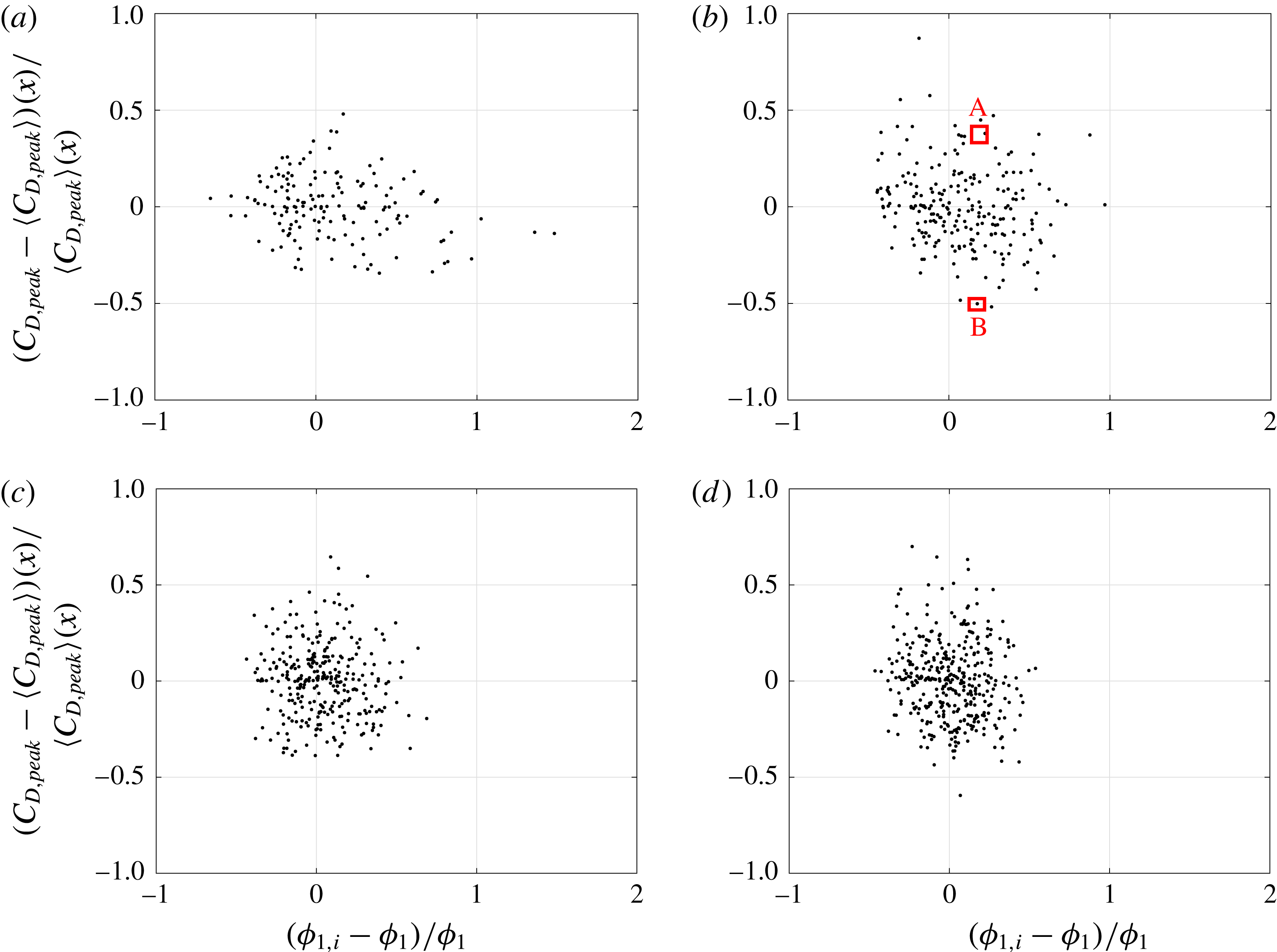
In figure 10 we plot the normalized variation in peak streamwise drag coefficient as a function of scaled local volume fraction. The normalized variation in peak drag coefficient is defined by
 $(C_{D,peak}-\langle C_{D,peak}\rangle )/\langle C_{D,peak}\rangle$
, where
 $C_{D,peak}$
is the peak drag coefficient for each particle and
 $\langle C_{D,peak}\rangle$
is the mean value shown by the red line in figure 8. The scaled local volume fraction is given by
 $(\unicode[STIX]{x1D719}_{1,i}-\unicode[STIX]{x1D719}_{1})/\unicode[STIX]{x1D719}_{1}$
. From the figure we see that increasing the global volume fraction from 10 % to 25 % decreases the spread in the local volume fraction, which is consistent with the statistics provided in table 1. However, with increasing global volume fraction, the spread in the fluctuating peak streamwise drag coefficient increases slightly. Contrary to expectation, this figure shows that the increase (or decrease) in the peak drag coefficient does not correlate with an increase (or decrease) in the local volume fraction. This observation is consistent with the findings of Akiki, Jackson & Balachandar (Reference Akiki, Jackson and Balachandar2016), who also noted that, in the case of a uniform steady incompressible flow over a random bed of particles, the deviation of the drag force on each particle from the bed-averaged mean does not correlate with the local volume fraction. In fact, other definitions of local volume fraction, such as number of particles within a large volume (Quintanilla & Torquato Reference Quintanilla and Torquato1997) or distance to the
 $n$
-nearest neighbour (Yazdchi, Srivastava & Luding Reference Yazdchi, Srivastava and Luding2012; Matsumura & Jackson Reference Matsumura and Jackson2014), can be used instead of the present definition based on local Voronoi volume. Nevertheless, local volume fraction as defined with all such isotropic definitions does not explain the particle-to-particle variation in the drag force (Akiki et al.
Reference Akiki, Jackson and Balachandar2016).
Plot of normalized peak streamwise drag coefficient,
 $(C_{D,peak}-\langle C_{D,peak}\rangle )/\langle C_{D,peak}\rangle$
, as a function of scaled local volume fraction (Voronoi volume),
 $(\unicode[STIX]{x1D719}_{i,1}-\unicode[STIX]{x1D719}_{1})/\unicode[STIX]{x1D719}_{1}$
, for (a)
 $\unicode[STIX]{x1D719}_{1}=10\,\%$
, (b)
 $\unicode[STIX]{x1D719}_{1}=15\,\%$
, (c)
 $\unicode[STIX]{x1D719}_{1}=20\,\%$
and (d)
 $\unicode[STIX]{x1D719}_{1}=25\,\%$
.

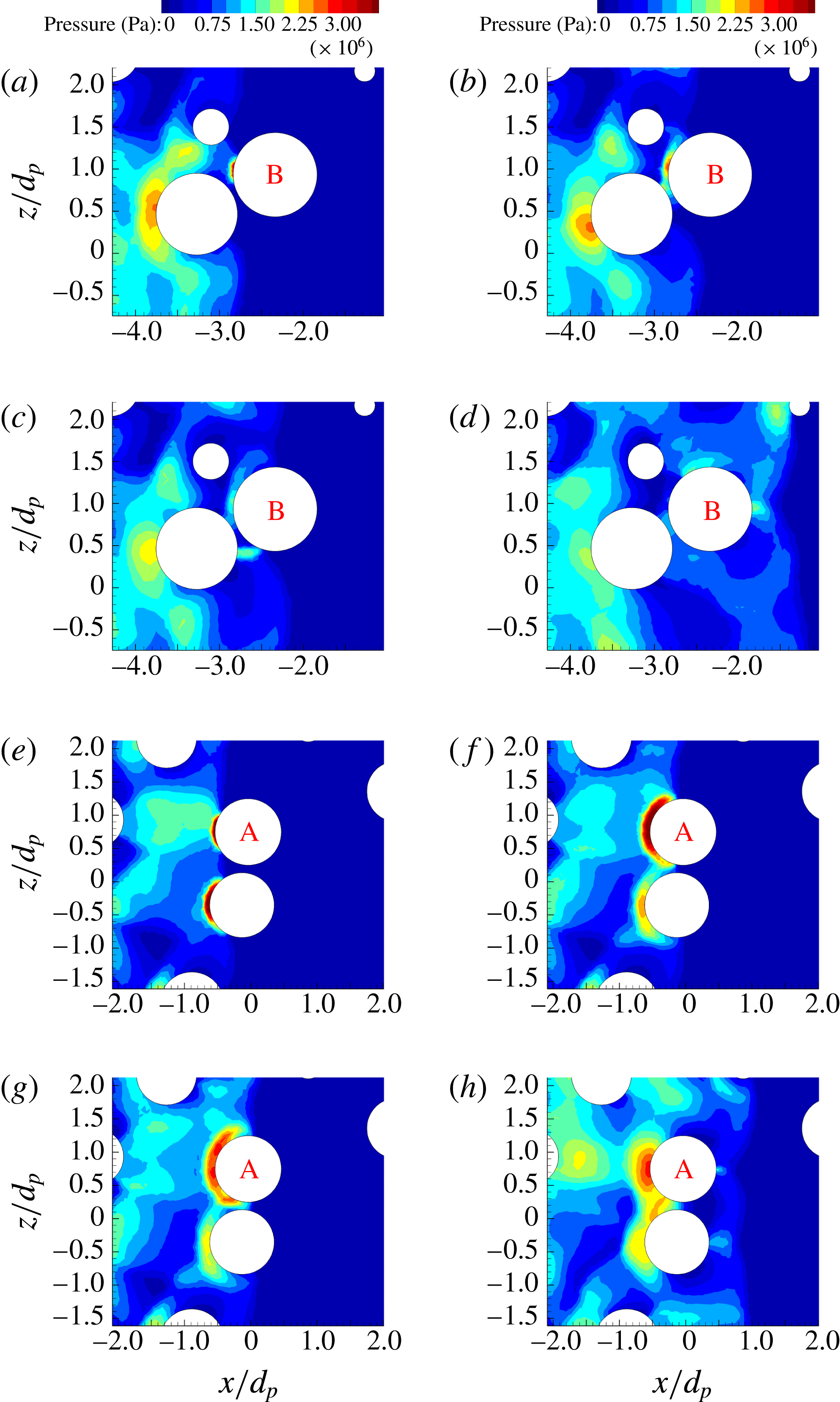
It is clear that two different particles with the same local volume fraction can have vastly different peak drag forces. For example, the two particles marked A and B in figure 10(b) have nearly the same local volume fraction, but their
 $C_{D,peak}$
are 1.9194 and 0.7251, respectively. The particle marked A experiences a peak drag force 45 % higher than the mean, while the particle marked B experiences a peak drag force 50 % lower than the mean. The neighbourhood and the resulting pressure fields around the two particles as the transmitted shock propagates through the neighbourhood of the two particles are shown in figure 11. It is clear that particle B is sheltered by another particle that is located directly upstream and close to it, thus decreasing the local strength of the transmitted shock encountering particle B, whereas particle A’s neighbours are located such that they help in focusing the transmitted shock as it encounters particle A. In both these cases the transmitted shock strength can be estimated from the pressure contours. Thus, the local volume fraction, or local Voronoi volume of a particle, is not an adequate measure (Akiki et al.
Reference Akiki, Jackson and Balachandar2016; Akiki, Jackson & Balachandar Reference Akiki, Jackson and Balachandar2017). A more precise knowledge of where the neighbouring particles (especially upstream neighbours) are located is critical in explaining higher or lower than mean drag forces experienced by the different particles within the bed (Boiko, Klinkov & Poplavskii Reference Boiko, Klinkov and Poplavskii2004; Wagner et al.
Reference Wagner, Beresh, Kearney, Trott, Castaneda, Pruett and Baer2012b
). Anisotropic measures of local neighbourhood involving distances to the nearest neighbours along the upstream, downstream and lateral directions were introduced by Akiki et al. (Reference Akiki, Jackson and Balachandar2016, Reference Akiki, Jackson and Balachandar2017), and these measures were shown to better correlate with the drag force experienced by the different particles.


Plot of streamwise drag coefficient,
 $C_{D}$
, as a function of shifted non-dimensional time,
 $(t-t_{arrival})/\unicode[STIX]{x1D70F}$
, and for volume fraction
 $\unicode[STIX]{x1D719}_{1}=15\,\%$
for (a) bin 1:
 $-8<x/d_{p}<-6$
, (b) bin 3:
 $-4<x/d_{p}<-2$
and (c) bin 5:
 $0<x/d_{p}<2$
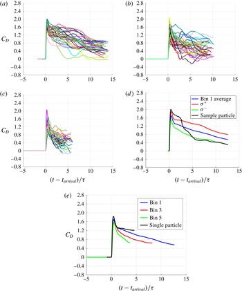
. (d) Force averaged over bin 1 along with the one sigma variation and the force on a sample particle. (e) Bin 1, bin 3, bin 5 averaged along with the force on a single particle.

We now investigate the time history of the mean drag force. In order to avoid the influence of the downstream shock decay, we calculate the mean drag force over bins of particles. We define each bin to be two diameters wide along the streamwise direction. Thus, the first bin will include all particles whose centre lies within
 $-8\leqslant x/d_{p}<-6$
, and correspondingly other bins are similarly defined. The force histories for particles in the first, third and fifth bins for
 $\unicode[STIX]{x1D719}_{1}=10\,\%$
are plotted in figure 12(a–c). It can be seen that the transmitted shock strength within each bin can be taken to be nearly uniform. The time history of
 $C_{D}$
presented in figure 12(a–c) for all the particles within the bin are sifted in time and averaged. The bin-averaged
 $C_{D}$
for bin 1 is shown in figure 12(d). Also plotted in the figure is one sigma variation, along with drag history of a sample particle from the random pack. It can be observed that the level of particle-to-particle variation seen in the peak value of
 $C_{D}$
persists over the entire duration of the simulation. However, as can be seen in the figure, there is no guarantee that the particle with the higher peak will continue to experience higher than mean force at later times. This is due to the fact that the neighbourhood configuration that was responsible for shock focusing and increased peak force may not present favourable conditions for increased drag during post-incident shock flow. Finally, figure 12(e) shows the time history of the bin-averaged force for 15 % volume fraction for bin 1, bin 3 and bin 5, along with the time history of force for an isolated particle subjected to Mach 3 incident shock. Note from the figure that the drag coefficient for a single particle is larger than for those for bins 1, 3 and 5, and that the peak and short-time transient downstream behaviour decreases monotonically as the bin number increases or, in other words, as the depth of the bed increases.
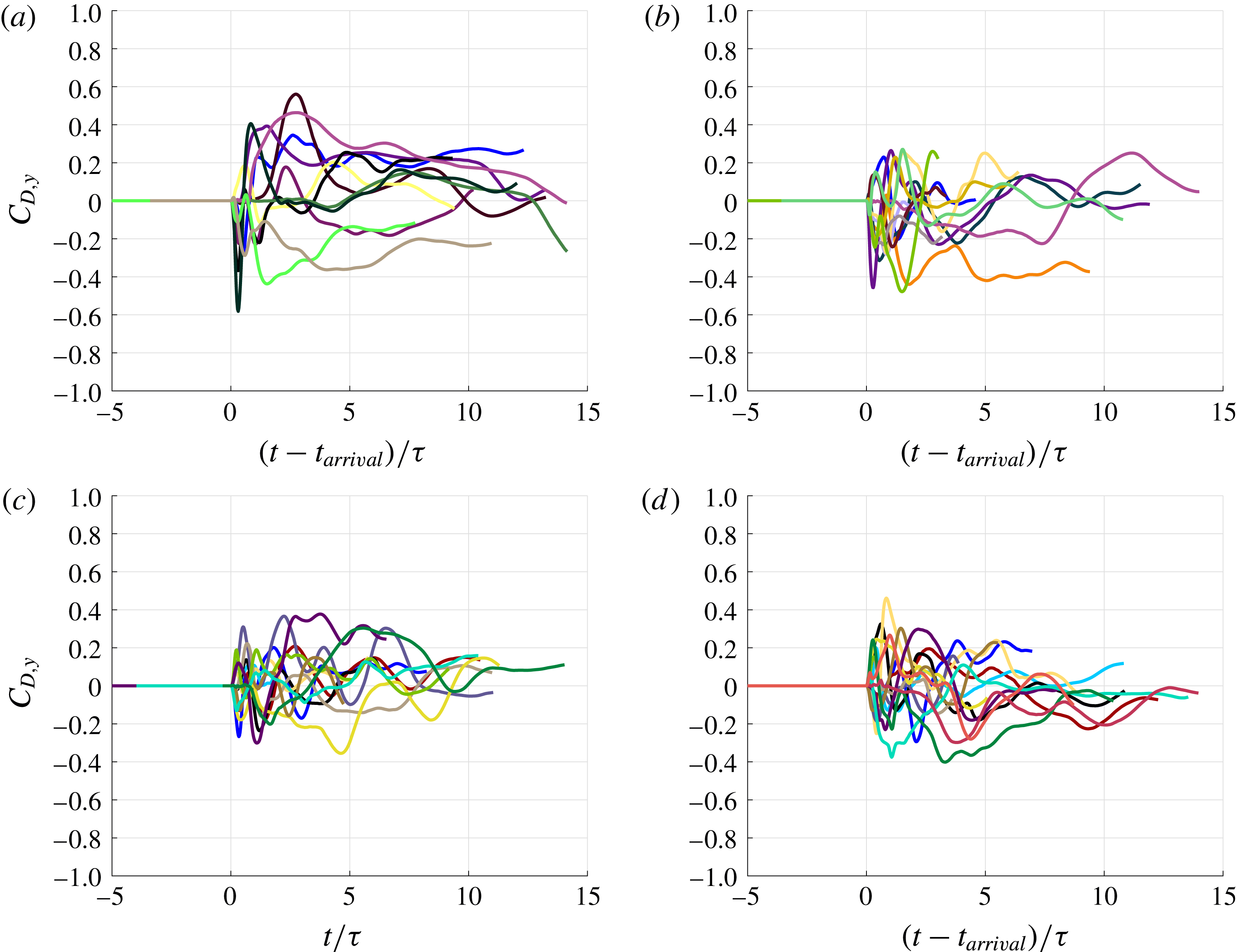
(a) Plot of transverse drag coefficient,
 $C_{D,y}$
, as a function of shifted non-dimensional time,
 $(t-t_{arrival})/\unicode[STIX]{x1D70F}$
, for a few representative particles and for volume fractions of (a)
 $\unicode[STIX]{x1D719}_{1}=10\,\%$
, (b)
 $\unicode[STIX]{x1D719}_{1}=15\,\%$
, (c)
 $\unicode[STIX]{x1D719}_{1}=20\,\%$
and (d)
 $\unicode[STIX]{x1D719}_{1}=25\,\%$
.

4.2 Transverse particle forces
In figure 13 we plot the
 $y$
-force on a few representative particles from the random pack for 10 %–25 % volume fractions. As in figure 7, the time axis has been shifted by the shock arrival time. The results for the force in the
 $z$
-direction show similar behaviour and are not shown here. From the plot we see that the mean transverse force, averaged over all the particles over time, will tend to zero, but that there are significant variations. As with the drag force, the transverse force coefficient is identically zero until the arrival of the transmitted shock. However, the transverse force due to the transmitted shock is significant only in situations where the shock is substantially oblique when it encounters the particle. In most other cases, the transverse force is due to the unsteady nature of the post-incident shock flow as a result of fluctuations generated by the random distribution of particles. Thus, not only the magnitude, but also the instance when the transverse force reaches a peak, varies strongly from particle to particle. It is also important to note that the transverse force can be 20 to 40 % of the streamwise force. Macroscale simulations of incident shock interaction with a point-particle model typically accounts for only the streamwise force on the particle bed. Even though the mean transverse force is zero, the strong instantaneous transverse force on the different particles is likely to play a role in both the shock transmission and the long-term motion of the bed of particles.
The total lift force or the transverse force is defined as
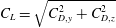 $C_{L}=\sqrt{C_{D,y}^{2}+C_{D,z}^{2}}$
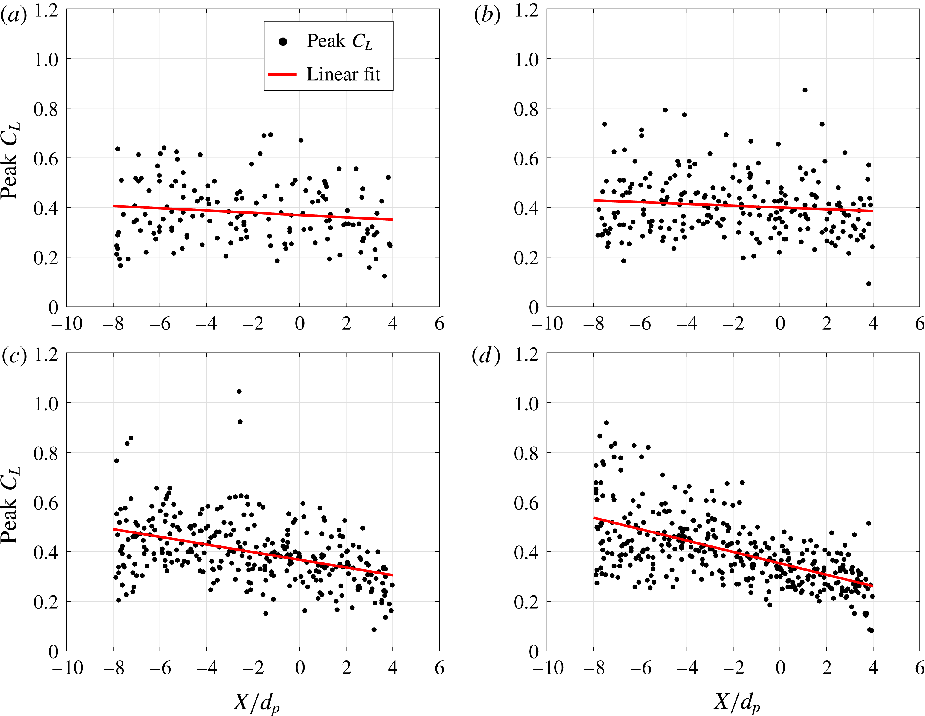
. Figure 14 plots the peak values
 $C_{L,peak}$
for all the particles as a function of their streamwise location. The linear curve shown in figure 14 is given by
 $\langle C_{L,peak}\rangle =q_{3}\unicode[STIX]{x1D709}/d_{p}+q_{4}$
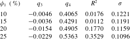
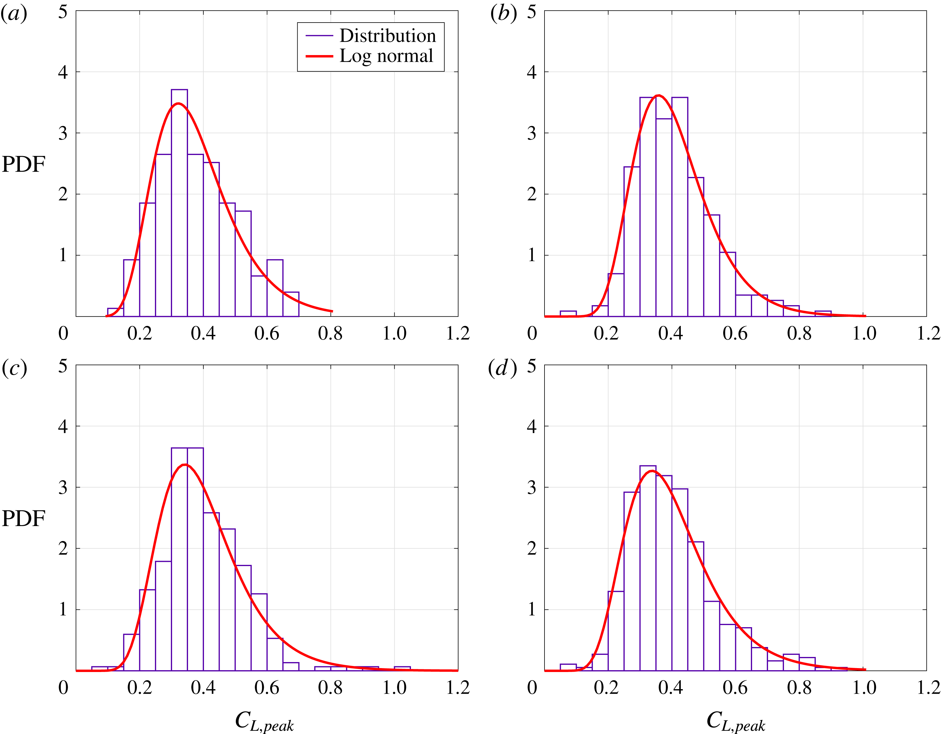
, with the statistics of the least-squares fit given in table 6. The slow decay of the peak transverse force along the streamwise direction is due to dissipation-induced shock weakening. The variability in the peak lift force is of the same magnitude as the variability in the drag force. However, since the mean transverse force is smaller, the relative importance of transverse force variability increases. The histograms of the transverse force variation are presented in figure 15. By definition
 $C_{L,peak}$
is non-negative and as a result the peak transverse force is positively skewed. The variations in peak transverse force are compared to a log-normal distribution in figure 15, and show a good overall fit to the data.
Plot of peak total transverse drag coefficient,
 $C_{L,peak}$
, for each particle. The red curve is the least-squares linear fit for the data. (a)
 $\unicode[STIX]{x1D719}_{1}=10\,\%$
, (b)
 $\unicode[STIX]{x1D719}_{1}=15\,\%$
, (c)
 $\unicode[STIX]{x1D719}_{1}=20\,\%$
and (d)
 $\unicode[STIX]{x1D719}_{1}=25\,\%$
.

Least-squares curve fit statistics for total transverse drag
 $C_{L,peak}$
.

Histogram of peak transverse drag coefficient,
 $C_{L,peak}$
. The red curve is the log-normal distribution fit for the data. (a)
 $\unicode[STIX]{x1D719}_{1}=10\,\%$
, (b)
 $\unicode[STIX]{x1D719}_{1}=15\,\%$
, (c)
 $\unicode[STIX]{x1D719}_{1}=20\,\%$
and (d)
 $\unicode[STIX]{x1D719}_{1}=25\,\%$
.

4.3 Flow fields
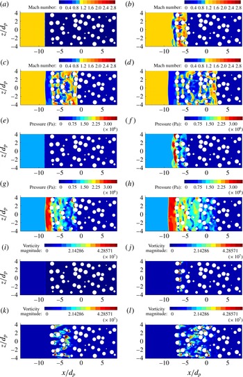
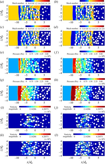
To highlight the flow dynamics as the incident shock propagates through a random pack of particles, in figures 16–17 we show contour plots of the local Mach number, pressure, and vorticity magnitude on the
 $x$
–
 $z$
plane at a fixed transverse (
 $y=0$
) location in the middle of the computational domain. The particles cut by this
 $x$
–
 $z$
plane are marked as white circles. Figure 16 plots contours at four different times and for a volume fraction of
 $\unicode[STIX]{x1D719}_{1}=15\,\%$
. The initial configuration and location of the incident shock are shown in figure 16(a). As time proceeds, the incident shock propagates downstream until it reaches the front of the particle bed. At later times a transmitted shock proceeds through the particle bed, which is visible in the Mach number contours shown in figure 16(b). At this early time, bow shocks can be seen to form ahead of the lead particles. A bow shock around an individual particle is expected to reach a steady stand-off distance from the particle, with the stand-off distance scaling as the size of the particle. In the case of a finite cluster of particles, a reflected shock forms from the coalescence of individual bow shocks. The reflected shock will propagate upstream to form a collective bow shock of the particle cluster (Boiko et al.
Reference Boiko, Klinkov and Poplavskii2004; Mehta et al.
Reference Mehta, Jackson, Zhang and Balachandar2016a
), whose stand-off distance from the cluster will scale as the lateral size of the cluster. In the present simulations, the particle bed is of infinite extent in the lateral directions, due to the symmetry boundary conditions along the
 $y$
and
 $z$
directions. Based on this we can expect the reflected shock to continue to move upstream and reach a constant propagation velocity, in agreement with the Riemann solution of the corresponding nozzle flow. The incident shock is strictly planar and the reflected shock is nearly planar once the bow shocks of the different lead particles coalesce into one. In contrast, the transmitted shock is corrugated as it propagates through the particle bed. But it can be observed that the length scale of these corrugations is smaller than the particle diameter. Thus, shock arrival time in a porous medium can be reasonably well approximated to be that of a planar shock.
After the passage of the transmitted shock, shocklets are seen to form around the particles, which can be identified as regions of higher Mach number in figure 16(f–h). The existence of these shocklets is a direct consequence of the flow being supercritical; i.e., the post-incident shock Mach number is locally greater than one. This observation is consistent with previous findings of an incident shock propagating through a FCC array (Mehta et al.
Reference Mehta, Neal, Jackson, Balachandar and Thakur2016b
). We note that the shocklets appear to connect nearest neighbours as the volume fraction increases beyond the dilute limit. In the pressure contour plots, substantial variation in the pressure distribution around particles that are at roughly the same streamwise location can be observed. Such differences in pressure distribution directly contribute to particle-to-particle variation in the streamwise and transverse drag forces. In interpreting these figures it must be borne in mind that only a single
 $x$
–
 $z$
plane is shown. Nearby particles that do not cut this
 $x$
–
 $z$
plane are not shown. However, such particles will have a strong influence on what is shown in these figures. As the transmitted shock weakens, the pressure drop across it also decreases. However, due to shock reflection the pressure is high in the region between the reflected shock and the upstream particle front. Also due to internal compressional waves and their constructive superposition, regions of high pressure can be seen within the particle bed, typically close to and upstream of the particles.
Contour plot of Mach number (a–d), pressure (e–h), and vorticity (magnitude) (i–l) along the
 $x$
–
 $z$
plane at
 $y=0$
for
 $M_{s}=3.0$
and
 $\unicode[STIX]{x1D719}_{1}=15\,\%$
at
 $t/\unicode[STIX]{x1D70F}=0$
(a,e,i),
 $t/\unicode[STIX]{x1D70F}=4$
(b,f,j),
 $t/\unicode[STIX]{x1D70F}=8$
(c,g,k) and
 $t/\unicode[STIX]{x1D70F}=12$
(d,h,l).

Contour plot of Mach number (a–d), pressure (e–h), and vorticity (magnitude) (i–l) along the
 $x$
–
 $z$
plane at
 $y=0$
for
 $M_{s}=3.0$
at
 $t/\unicode[STIX]{x1D70F}=12$
for
 $\unicode[STIX]{x1D719}_{1}=10\,\%$
(a,e,i),
 $\unicode[STIX]{x1D719}_{1}=15\,\%$
(b,f,j),
 $\unicode[STIX]{x1D719}_{1}=20\,\%$
(c,g,k) and
 $\unicode[STIX]{x1D719}_{1}=25\,\%$
(d,h,l).

Since the simulations are inviscid, the vorticity (magnitude) shown in figure 16(j–l) is baroclinic in origin. In a viscous simulation additional vorticity will be generated on the surface of the sphere due to no-slip boundary condition. As mentioned in § 2.6, for an isolated particle under the same incident shock conditions, negligible vorticity is generated in the present inviscid simulations. In fact the vorticity magnitude for a single particle is at least two orders of magnitude less than that observed in figure 16(j–l). Thus the vorticity seen in figure 16(j–l) is not due to numerical viscosity. It appears that the baroclinic vorticity production is amplified when symmetry is broken by randomly distributed particles. It is interesting to note that most of the vorticity is in the wake region behind the particles. The downstream particles are thus subjected to vorticity generated by the upstream particles. The deformation of the advected vorticity around the downstream particle contributes to rotational forces on the particle (Eames & Hunt Reference Eames and Hunt1997; Auton, Hunt & Prud’Homme Reference Auton, Hunt and Prud’Homme1988), whose magnitude can be estimated in terms of
 $\boldsymbol{u}\times \unicode[STIX]{x1D74E}$
, where
 $\boldsymbol{u}$
and
 $\unicode[STIX]{x1D74E}$
are the undisturbed velocity and vorticity at the particular location.
Figure 17 plots similar quantities but at a fixed time and for different volume fractions. Several points should be noted. First, the upstream propagation speed of the reflected shock is in general small, but the shock appears to form more quickly and travel upstream faster as the volume fraction increases. Comparing with the results of the Riemann problem shown in figure 6, it can be observed that the speed of the reflected shock is higher for the larger-area-reduction cases. The terminal Mach number of the reflected shock,
 $M_{r}$
, is presented in table 7, which can be compared with that shown in table 4 for the Riemann problem. It can be seen that the strength of the reflected shock, computed from numerical simulations, is slightly higher than that predicted by the one-dimensional Riemann theory.
Flow properties across the domain from numerical simulations for different volume fractions;
 $M_{s}=3$
and
 $t/\unicode[STIX]{x1D70F}=12$
.

4.4 Shock attenuation through the particle bed
In this section we plot
 $y$
–
 $z$
-averaged flow quantities in the computational domain to determine, among other things, the strength of the transmitted shock. These cross-stream-averaged plots can be compared to those of the Riemann problem in order to better understand the impact of the particles on the flow, and to investigate the pressure attenuation or local amplification behind the particle (porous) barrier.
To compute averaged flow quantities, the computational domain is decomposed into 200 individual
 $y$
–
 $z$
slices. The flow field variables on the slices are then averaged to obtain a mean value of the quantities on the slice. This process yields a discrete set of averaged flow quantities that vary with time and the streamwise
 $x$
-direction. If a flow variable is denoted as
 $F(x,y,z,t)$
, then the process for determining the averaged value of the flow field variable on a slice is given by
 $$\begin{eqnarray}\langle F\rangle (x,t)=\frac{1}{A_{g}}\int _{L_{y}}\int _{L_{z}}I_{g}(x,y,z)F(x,y,z,t)\,\text{d}y\,\text{d}z,\end{eqnarray}$$
where
 $L_{y}$
and
 $L_{z}$
are the size of the computational domain along the transverse directions. Here,
 $I_{g}(x,y,z)$
is the indicator function that identifies only the region occupied by the gas, outside the particle volume (i.e.,
 $I_{g}=1$
in the gas and
 $I_{g}=0$
inside the particle). Thus, the integral is only over the cross-sectional area occupied by the gas, and correspondingly
 $A_{g}=\int _{L_{y}}\int _{L_{z}}I_{g}(x,y,z)\,\text{d}y\,\text{d}z$
is the cross-sectional area occupied by the gas.
The cross-stream-averaged pressure, density, and
 $(u,v,w)$
velocity components normalized by post-incident shock values are shown in figures 18–20, respectively, and for the four volume fractions considered in this study. Here we consider the flow field results from the 200 two-dimensional slices. Four representative times are used to show the evolution of the averaged flow field with time as the transmitted shock passes through the particle bed. Note that all four cases of volume fraction have the same post-incident shock properties in the absence of a particle bed (i.e., same state
 $\unicode[STIX]{x2465}$
), so the deviation from this state indicates how the flow in each particle bed differs.
Plot of non-dimensionalized streamwise-averaged pressure,
 $\langle p\rangle /p_{6}$
, in the random particle bed at four times and for (a)
 $\unicode[STIX]{x1D719}_{1}=10\,\%$
, (b)
 $\unicode[STIX]{x1D719}_{1}=15\,\%$
, (c)
 $\unicode[STIX]{x1D719}_{1}=20\,\%$
and (d)
 $\unicode[STIX]{x1D719}_{1}=25\,\%$
. Times shown are
 $t/\unicode[STIX]{x1D70F}=0$
(red),
 $t/\unicode[STIX]{x1D70F}=4$
(green),
 $t/\unicode[STIX]{x1D70F}=8$
(blue) and
 $t/\unicode[STIX]{x1D70F}=12$
(black). The location of the incident shock at
 $t/\unicode[STIX]{x1D70F}=0$
is approximately at
 $x/d_{p}=-9$
. The particle bed begins at approximately
 $x/d_{p}=-8$
.

Plot of non-dimensionalized streamwise-averaged density,
 $\langle \unicode[STIX]{x1D70C}\rangle /\unicode[STIX]{x1D70C}_{6}$
, in the random particle bed at four times and for (a)
 $\unicode[STIX]{x1D719}_{1}=10\,\%$
, (b)
 $\unicode[STIX]{x1D719}_{1}=15\,\%$
, (c)
 $\unicode[STIX]{x1D719}_{1}=20\,\%$
and (d)
 $\unicode[STIX]{x1D719}_{1}=25\,\%$
. Times shown are
 $t/\unicode[STIX]{x1D70F}=0$
(red),
 $t/\unicode[STIX]{x1D70F}=4$
(green),
 $t/\unicode[STIX]{x1D70F}=8$
(blue) and
 $t/\unicode[STIX]{x1D70F}=12$
(black).

Plot of non-dimensionalized streamwise-averaged velocity,
 $\langle u\rangle /u_{6}$
, in the random particle bed at four times and for (a)
 $\unicode[STIX]{x1D719}_{1}=10\,\%$
, (b)
 $\unicode[STIX]{x1D719}_{1}=15\,\%$
, (c)
 $\unicode[STIX]{x1D719}_{1}=20\,\%$
and (d)
 $\unicode[STIX]{x1D719}_{1}=25\,\%$
. Times shown are
 $t/\unicode[STIX]{x1D70F}=0$
(red),
 $t/\unicode[STIX]{x1D70F}=4$
(green),
 $t/\unicode[STIX]{x1D70F}=8$
(blue) and
 $t/\unicode[STIX]{x1D70F}=12$
(black).

The transmitted shock front can be seen in figure 18 as the location where the pressure rises rapidly from the ambient pressure state, which is the constant state on the right side of these figures. Since all quantities are scaled by their post-incident shock value, and thus ahead of the reflected shock, all normalized quantities reach a constant value of 1.0 on the left. For 10 % volume fraction, the pressure distribution shown in red of figure 18(a) is the initial condition with the incident shock placed upstream of the particle bed. Hence the region between shocked and unshocked is clearly marked with a sharp pressure discontinuity. As the incident shock moves into the particle bed (green, blue, black) a coalesced bow shock begins to form upstream of the particle bed. The presence of this coherent bow shock can be seen as the steep pressure rise above the post-incident shock pressure ahead of the particle bed. For the 15 % volume fraction case, we can see in figure 18(b) that the pressure distributions are qualitatively similar to those in figure 18(a). The effect of the higher volume fraction in the bed can be seen in the peak upstream pressure increasing by approximately 20 % compared to the peak in figure 18(a). In both these lower volume fraction cases, the pressure across the reflected shock continues to increase over the range of time considered. Thus, it can be concluded that the reflected shock is still developing towards a quasistationary state. For the 20 % volume fraction case shown in figure 18(c), we can see that the pressure distributions are qualitatively similar to those of 10 % and 15 %. However, the pressure increase across the reflected shock upstream of the particle bed has reached a steady value, which is indicated by the near-constant flat pressure distribution between the reflected shock and the front of the particle bed. This flattened peak is approximately 40 % higher than the peak pressure of the 10 % volume fraction case. This increase in pressure between the reflected shock and the front of the particle bed with increasing particle volume fraction is in qualitative agreement with the corresponding behaviour seen in the Riemann problem for sudden area reduction. The pressure ratios are given in table 7 for the four different volume fractions, which can be compared against the corresponding values presented in table 4 for the Riemann problem. From figure 18, note that the growth of the coalesced bow shock is faster with increasing volume fraction. But this temporal development through coalescence of individual bow shocks is only a feature of the particle bed, as the reflected shock instantly forms in the case of the Riemann problem. Furthermore, the temporal development only pertains to the peak pressure, since in figure 18 the location of the reflected shock can be observed to steadily move upstream in all the cases considered. Similar to the previous pressure plot for 20 % volume fraction, we see that the peak upstream pressure across the reflected shock increases and plateaus in figure 18(d) for 25 % volume fraction.
The pressure drops rapidly across the front face of the particle bed, which can be clearly observed in the higher volume fraction cases. The pressure continues to fall steadily across the bed and the pressure gradient increases with volume fraction. The pressure gradient within the bed appears to be nearly a constant in the high-volume-fraction cases, while in the low-volume-fraction cases the gradient seems to be slightly larger close to the front face of the particle bed.
The pressure jump on the right seen in all the plots is due to the transmitted shock. The pressure change across the transmitted shock front in all the cases experiences a decay with time as the transmitted shock front moves through the particle bed. Also, unlike the reflected shock, the pressure jump across the transmitted shock appears to occur over a region of finite thickness. From the Mach number contours shown in figures 16 and 17 it is clear that the transmitted shock is not planar. The undulations in the transmitted shock front as it diffracts around the bed of particles is responsible for the apparent finite thickness of the transmitted shock.
Figure 19 shows the density variation with
 $x/d_{p}$
at four different times for the four different particle bed volume fractions considered in this study. The density profiles are quite similar to those of pressure shown in figure 18. Again the signature of the reflected shock can be seen as the rapid increase in density upstream of the particle bed. The density of the gas rapidly decreases as it enters the particle bed, which is most evident at the higher volume fraction. Again the density linearly decreases within the upstream portion of the bed, and reaches a near-constant value ahead of the transmitted shock. This behaviour is entirely consistent with the density plot of the Riemann solution presented in figure 6. The region of linear density variation within the bed denotes the presence of a resonant expansion fan, whose thickness increases over time. However, such a constant state is not observed in the pressure distribution, since the decrease in pressure within the bed is due to both the resonant expansion fan and shocklet-induced energy dissipation. Nevertheless, the presence of a contact discontinuity cannot be discerned in the density plots, due to the very small value of the density jump that can be expected from the Riemann problem. The density jump seen in figure 19 across the reflected shock is consistent with the reflected shock Mach number presented in table 7, and similarly the density jump across the transmitted shock is consistent with the transmitted shock Mach number presented in table 7.
The normalized streamwise velocity profiles are shown in figure 20. Here the velocity drops across the reflected and the transmitted shocks. As can be expected, the streamwise velocity increases sharply as the flow enters the bed of particles. Within the bed itself the velocity continues to increase. This increase is partially due to the resonant expansion fan and partially due to the dissipative decrease in pressure. We also calculated cross-stream-averaged
 $y$
and
 $z$
components of velocities (but not shown here). They are typically limited to only 2 % to 3 % of the mean streamwise velocity. From statistical considerations we expect the ensemble-averaged transverse velocities to be zero, and thus their small non-zero values are indicative of the effect of the finite dimension of the computational domain in the
 $y$
and
 $z$
directions. With a larger computational domain in the transverse directions the mean
 $y$
and
 $z$
velocities can be further decreased; however, the computational cost will increase as well.
Ratios of pressure, density, and velocity behind the transmitted shock normalized by the post-incident shock properties (
 $P_{2}/P_{6}$
,
 $\unicode[STIX]{x1D70C}_{2}/\unicode[STIX]{x1D70C}_{6}$
, and
 $u_{2}/u_{6}$
) are presented in table 7. These ratios help us quantify the dissipation inside the particle bed, since in the absence of particles the incident shock will be the transmitted shock. Note that the flow properties behind the transmitted shock in the case of the Riemann problem are nearly equal to the post-incident shock properties. Also given in table 7 is the strength of the transmitted shock,
 $M_{t}$
, which can be compared with the Mach number of the transmitted shock for the Riemann problem given in table 4. It is clear that the strength of the transmitted shock decreases as the volume fraction increases. We see from the table that the pressure drop,
 $P_{2}/P_{6}$
, across the particle bed varies between 13 % for
 $\unicode[STIX]{x1D719}_{1}=10\,\%$
to 33 % for
 $\unicode[STIX]{x1D719}_{1}=25\,\%$
. Thus, there is a significant drop in the post-shock pressure of the transmitted shock front. This trend is consistent with the observed drop in the peak particle drag coefficients shown in figure 8. This decay of the transmitted shock is due to the added dissipation within the bulk of the particle bed, which will be further discussed in the following section.
4.5 Approach to equilibrium
The nozzle flow considered in § 3 is similar to the problem of incident shock propagation through a bed of particles, except for the inviscid drag induced on the particles within the bed and the corresponding feedback effect on the flow. In the case of the one-dimensional nozzle flow shown in figure 4, the reflected and the transmitted shocks form very rapidly and propagate at constant velocity without any decay, and thus the one-dimensional nozzle flow can be considered to have reached its equilibrium state. A few additional points should be noted. In the inviscid nozzle limit there is dissipation of energy only at the reflected and the transmitted shocks, but the rate of energy dissipation remains a constant, since the reflected and the transmitted shock strengths remain the same over time; i.e., the reflected and the transmitted shocks are steady in respective frames attached to them. The equilibrium state of shock propagation in a one-dimensional nozzle flow is possible only when the dissipation rate is a constant. From figure 6 it is clear that the reflected shock will continue to move upstream at a constant speed, which is substantially lower than the speed of the transmitted shock.
The most significant difference between the one-dimensional nozzle solution and the results shown in figures 18 to 20 is the continued decay of the transmitted shock as it propagates deeper inside the particle bed. In contrast, the transmitted shock in the one-dimensional nozzle is of constant strength. The difference between the two configurations is the presence of shocklets within the particle bed as the near-uniform flow behind the transmitted shock negotiates around the random distribution of particles. These shocklets contribute to energy dissipation within the particle bed, which is in addition to dissipation that occurs at the reflected and transmitted shocks. As the transmitted shock propagates deeper into the particle bed, an increasing region of shocklets and energy dissipation forms within the bed swept by the transmitted shock. Thus, unlike in the one-dimensional nozzle flow, where dissipation is limited to the reflected and the transmitted shocks and therefore remains a constant over time, in the case of a particle bed the rate of dissipation increases over time. This increasing total dissipation rate is related to (i) the steady reduction in the strength of the transmitted shock, (ii) the enhanced pressure gradient within the particle bed (in the one-dimensional nozzle flow the pressure gradient is only across the resonant expansion fan), and (iii) the net positive inviscid drag experienced by the particles over long time well after the passage of the transmitted shock.
We now can investigate conditions under which an equilibrium state will be approached in the case of incident shock propagation over a bed of particles. When the particle bed is of finite thickness (in other words in case of incident shock propagation past a frozen particle curtain), we can expect an equilibrium state to be approached over a very long time. In this scenario the incident shock will first experience an area reduction as it encounters the particle curtain. The resulting transmitted shock will experience an increase in area as it passes out of the curtain. The Riemann solution to the first problem of area reduction has been discussed in § 3, and the Riemann solution for the second problem of shock propagation into an expansion can be obtained similarly. We expect another set of transmitted and reflected waves for this case as well. The reflected waves which propagate into the bed of particles will interact with the forward propagating contact discontinuity and the expansion fan, before reaching the front face of the particle bed. Similar reflections will occur for the contact as well as the expansion fan as they reach the back end of the particle bed. Over time there will be repeated reflections of waves inside the particle bed, with each reflection contributing to possible transmitted waves. The strength of these reflections decays over time and a final quasiequilibrium state for the original reflected and the original transmitted shocks can be expected. This quasiequilibrium state will depend on the net rate of dissipation that occurs within the bed of particles, which will approach a steady value as the internal reflections decay over time.
Two other factors that were not considered in the present simulations will affect the equilibrium state and its approach. It is appropriate to include viscous effects to represent the flow within the particle bed, even when the high-speed flow away from the particle bed can be satisfactorily represented by the Euler equations. The added viscous effect will enhance the aerodynamic force on the particles, both during the transient state when the transmitted shock and the subsequent internally reflected waves propagate through the bed, and during the long-term stationary state well after the passage of the transmitted shock. The enhanced dissipation within the bed of particles will decrease the equilibrium strengths of the reflected and transmitted shocks.
The relative importance of the viscous drag within the particle bed depends on the strength of the incident shock. For a supercritical post-incident shock Mach number (0.6 for a sphere), there is shocklet-induced dissipation, which will be amplified by the viscous effects. With increasing incident shock Mach number the viscous contribution to dissipation and drag will become smaller. On the other hand, as the incident shock Mach number decreases below a certain critical value (which may depend on the particle volume fraction of the bed) the flow within the bed after the passage of the transmitted shock will remain entirely subsonic and subcritical. In that case, the entire dissipation and drag on the particles is due to viscous effects. At such weak incident shock Mach numbers, an inviscid simulation result can be expected to be in closer agreement with the one-dimensional nozzle theory, as there is no added dissipation within the particle bed.
Substantial differences arise if the bed of particles is allowed to move downstream in response to the aerodynamic forces exerted on it (Ling et al. Reference Ling, Wagner, Beresh, Kearney and Balachandar2012; Wagner et al. Reference Wagner, Beresh, Kearney, Trott, Castaneda, Pruett and Baer2012b ). If the particle inertia is large, the particle acceleration will be small and the velocity of the bed may not be significant until the transmitted shock is far downstream of the bed. Thus, as long as the transmitted shock is within the particle bed or only a short distance downstream, the results for a freely moving particle may still be close to those for a stationary bed. Over long time, two effects contribute to a substantially different behaviour. As the particles within the bed start to move downstream, the relative velocity between the particles and the surrounding gas decreases. As a result, both the inviscid and viscous drag on the particles decrease over time, which will in turn modify the reflected and transmitted shocks. Also, experiments and simulations have shown that the thickness of the particle bed increases over time (Ling et al. Reference Ling, Wagner, Beresh, Kearney and Balachandar2012; Wagner et al. Reference Wagner, Beresh, Kearney, Pruett and Wright2012a ,Reference Wagner, Beresh, Kearney, Trott, Castaneda, Pruett and Baer b ), which will also influence the strength of the reflected and transmitted shocks.
Finally, let us consider the situation when the thickness of the particle bed is large. If we first restrict our attention to a strong incident shock in the inviscid limit, the following scenario can be envisioned. As the transmitted shock propagates through the bed, its strength decreases due to shocklet-induced dissipation. As the transmitted shock strength decreases, there will be a location (
 $L_{crit}$
) within the bed where the transmitted shock strength is sufficiently low that the flow after the transmitted shock passage is subcritical and does not support any internal shocklets within the bed. In this case, dissipation within the bed is limited to only upstream of
 $L_{crit}$
and the extent of the bed beyond this point is unimportant. The transmitted shock strength at the very beginning will be as predicted by one-dimensional nozzle theory, but it will steadily decrease until the transmitted shock reaches
 $L_{crit}$
. Beyond this point, the transmitted shock strength will remain the same (as there is no additional dissipation), which is its inviscid equilibrium state. Correspondingly, the reflected shock will reach its equilibrium state as well. This equilibrium picture is pertinent only in an inviscid simulation. With viscous effects taken into account, the dissipation rate will continue to increase within the bed and an equilibrium state cannot exist in the case of a very thick bed. The transmitted shock will be fully dissipated.
5 Conclusions
An investigation of a strong incident shock propagating through a random bed of spherical particles was presented. Three-dimensional numerical simulations were carried out and results for varying volume fraction at a fixed incident shock Mach number were given. We computed the unsteady inviscid streamwise and transverse drag coefficients for each particle in the random bed and found that the drag for each particle is strongly influenced by its neighbouring particles. Fluid-mediated particle–particle interaction leads to significant variation in drag force for each particle compared to the force history of a single particle. We show that the peak streamwise drag coefficient decreases as a function of streamwise distance through the random bed. This decrease in peak drag force is a result of weakening transmitted shock because of dissipation at shocklets and bow shocks that form around the particles.
We compare the drag force experienced by randomly distributed particles against the drag force experienced by particles arranged in structured arrays to highlight the effect of random distribution. For all the cases that we have considered, the mean drag force for the random bed of particles is less than the drag force by the particles in the structured array, even though some particles in the random bed have peak drag force comparable to that of the structured array. We have computed the local volume fraction around each particle by means of Voronoi tessellation, and show significant variation in the local volume fraction. Knowledge of such information is useful when understanding the influence of nearest neighbours on global flow quantities such as drag. Traditional drag models include a volume fraction correction term to account for drag variation due to the effect of volume fraction (Ashok S. Sangani & Prosperetti Reference Ashok S. Sangani and Prosperetti1991). We show that there is no correlation between the local volume fraction and the variation in the drag force. There is a need for anisotropic measure of local volume fraction, which can inform the precise arrangement of neighbouring particles to capture the drag variation based on this local particle arrangement. We also show that when properly scaled, the particle–particle variation of the peak streamwise drag coefficient can be well represented by a normal distribution. This information can be used to develop better force models for predicting the drag force experienced by a bed of particles.
We also plotted the local Mach number and pressure contours for various volume fractions to explain the observed complex physical mechanisms occurring during the shock–particle interactions. Vorticity magnitude was computed to highlight the baroclinic generation of vorticity and its effect on the particles. Since the incident shock interaction with the random bed of particles leads to transmitted and reflected waves, we compute the average pressure to characterize the strength of the transmitted shock wave to study pressure attenuation through the particle bed. We recast the problem of an incident shock interacting with a bed of particles as an incident shock interacting with a one-dimensional duct with area change. We obtained the Riemann solution for shock evolution for this set-up. Four different wave structures were identified using the Riemann solution, which included the transmitted shock, reflected shock, contact discontinuity and a resonant expansion wave attached to the location of area change. The effect of randomly distributed particles on the strength and dynamics of these wave structures was computed by comparing the Riemann solution against the numerical simulation results. This comparison was helpful in understanding the attenuation of the incident shock as it travelled through the bed of particles and the possible existence of an equilibrium state for this complicated problem. Future work will include viscous effects as well as particle movement and different distributions of particles.
Acknowledgements
This work was performed under the auspices of the U.S. Department of Energy by Lawrence Livermore National Laboratory under contract DE-AC52-07NA27344 (IM#LLNL-TR-729310). This work was also supported in part by the U.S. Department of Energy, National Nuclear Security Administration, Advanced Simulation and Computing Program, as a Cooperative Agreement under the Predictive Science Academic Alliance Program, under contract DE-NA0002378. T.L.J. was also supported in part by the Defense Threat Reduction Agency, Basic Research Award no. HDTRA1-14-1-0031 to University of Florida; S.B. was also supported in part by the Defense Threat Reduction Agency, Basic Research Award no. HDTRA1-14-1-0028 to University of Florida.