1 Introduction
Despite a large amount of studies, wall turbulence remains one of the subjects of classical physics and engineering that requires improved understanding. Over the last decades, research in wall turbulence has mainly focused on reaching higher Reynolds numbers (
 $Re$
). Recent laboratory and numerical experiments have concentrated on the existence of energetic large-scale structures (Jiménez Reference Jiménez1998) and their modulation effect on small scales (Marusic, Mathis & Hutchins Reference Marusic, Mathis and Hutchins2010; Schlatter & Örlü Reference Schlatter and Örlü2010b
). At the other end of the
 $Re$
range, one can define a Reynolds number
 $Re_{g}$
, below which no turbulence is sustained in the long-time limit. Understanding the dynamics of turbulence close to
 $Re_{g}$
appears also of fundamental importance, because it would shed light on the self-sustenance mechanisms of wall turbulence themselves. Studying turbulence at these relatively low values of
 $Re$
has for instance helped to unravel the mechanisms at play during the regeneration of coherent structures in the near-wall region (Hall & Smith Reference Hall and Smith1991; Jiménez & Moin Reference Jiménez and Moin1991; Hamilton, Kim & Waleffe Reference Hamilton, Kim and Waleffe1995).
The study of wall turbulence near its onset is notoriously difficult because it requires a spatio-temporal description. Far above
 $Re_{g}$
, initially localised disturbances spread spatially and turbulence invades the whole domain (Emmons Reference Emmons1951; Henningson, Spalart & Kim Reference Henningson, Spalart and Kim1987). Closer to, but still above,
 $Re_{g}$
, turbulence can partially collapse, so that the turbulent regime is no longer space-filling. Such partial collapse events can bring the flow into a sustained spatio-temporal intermittency (STI) regime characterised by a stochastic sequence of local relaminarisation events balanced by turbulence contamination (Chaté & Manneville Reference Chaté, Manneville, Tabeling and Cardoso1994), as observed in pipe flow (Avila et al.
Reference Avila, Moxey, de Lozar, Avila, Barkley and Hof2011). The critical point
 $Re=Re_{g}$
corresponds to the value of the control parameter below which global collapse, rather than local collapse of turbulence, occurs over unlimited observation times with unit probability. In practice, however, rather than STI, the regimes found in most planar shear flows above
 $Re_{g}$
display a more spatially ordered coexistence akin to pattern formation: robust laminar–turbulent interfaces appear oblique with respect to the mean direction of the flow, laminar zones having relatively well-determined lengths. This patterning phenomenon was first observed experimentally in counter-rotating regimes of Taylor–Couette flow (Coles Reference Coles1965; Hegseth et al.
Reference Hegseth, Andereck, Hayot and Pomeau1989; Prigent Reference Prigent2001), and the structure was named ‘barber-pole turbulence’. Similar phenomena were later described in rotor–stator flow (Cros & Le Gal Reference Cros and Le Gal2002), as well as in plane Couette flow and plane Poiseuille flow using both laboratory and numerical experiments (Prigent et al.
Reference Prigent, Grégoire, Chaté, Dauchot and van Saarloos2002; Barkley & Tuckerman Reference Barkley and Tuckerman2005; Tsukahara et al.
Reference Tsukahara, Seki, Kawamura and Tochio2005; Duguet, Schlatter & Henningson Reference Duguet, Schlatter and Henningson2010). Philip & Manneville (Reference Philip and Manneville2011) obtained a comprehensive bifurcation diagram for plane Couette flow and specified the range of Reynolds numbers above
 $Re_{g}$
where pattern formation is found. They highlighted minimum size requirements for the numerical domain, linked to the large wavelength of the patterns. Brethouwer, Duguet & Schlatter (Reference Brethouwer, Duguet and Schlatter2012) showed that the patterned regime can be shifted to higher
 $Re$
by the addition of an external forcing stabilising the flow, e.g. system rotation, buoyancy or Lorentz forces. Recently, regimes of patterned turbulence were also identified in stratified boundary-layer flows (Ansorge & Mellado Reference Ansorge and Mellado2014; Deusebio et al.
Reference Deusebio, Brethouwer, Schlatter and Lindborg2014). Duguet & Schlatter (Reference Duguet and Schlatter2013) suggested a mechanism justifying the obliqueness of laminar–turbulent interfaces for generic planar shear flows. It relies on the existence of a large-scale flow forming near possible laminar–turbulent interfaces because of the mismatch of flow rates across them. Deceleration inside the turbulent regions implies by mass conservation the existence of a large-scale spanwise flow. The resulting large-scale flow advects the weakest turbulent fluctuations along the interface, which contributes over long times to the robust emergence of an oblique large-scale pattern. Similar analysis was put forward by Seki & Matsubara (Reference Seki and Matsubara2012).
The feature common to all these shear flows, justifying de facto a statistical description in terms of phase transition and spatio-temporal intermittency concepts (Manneville Reference Manneville2009; Moxey & Barkley Reference Moxey and Barkley2010; Lemoult et al.
Reference Lemoult, Shi, Avila, Jalikop, Avila and Hof2016), is the linear stability of the laminar base flow. When this stable base flow is in competition with a nonlinear self-sustenance mechanism (Hamilton et al.
Reference Hamilton, Kim and Waleffe1995), there is a finite probability for local turbulence collapse near
 $Re_{g}$
. The regularised patterns of laminar–turbulent coexistence result from the complex longer-range interactions associated with the planar large-scale flow.
In this work we investigate turbulence close to its onset in boundary-layer flows, where concepts of STI as an equilibrium regime (excluding effects of incoming turbulence) were not given as much attention. Spatially developing boundary layers, such as Blasius or Falkner–Skan–Cooke flows, are poorly adapted to this point of view as there is no external control parameter (the Reynolds number is actually space-dependent and serves as a measure of the downstream distance). One option is to apply weak suction at the wall in order to counteract the spatial growth and render the flow parallel. If the suction velocity
 $V_{S}$
is constant in time and homogeneous in space, the boundary-layer thickness eventually equilibrates, making the flow independent of the streamwise direction. In this case the flow is called the asymptotic suction boundary-layer (ASBL) flow (see Schlichting Reference Schlichting1987). Unlike spatially developing flows, it is characterised by a genuine control parameter, a Reynolds number commonly built on the properties of the laminar solution and inversely proportional to
 $V_{S}$
.
Apart from being one of the few analytical solutions to the incompressible Navier–Stokes equations, ASBL is also realisable in experiments using a porous plate (Antonia et al.
Reference Antonia, Fulachier, Krishnamoorthy, Benabid and Anselmet1988; Fransson & Alfredsson Reference Fransson and Alfredsson2003). Although suction is known to lead to turbulent drag enhancement (Kametani et al.
Reference Kametani, Fukagata, Örlü and Schlatter2015), it is a way to delay transition to higher
 $Re$
. Indeed, homogeneous suction reduces the growth rate of the Tollmien–Schlichting waves (Reynolds & Saric Reference Reynolds and Saric1986; Schlichting Reference Schlichting1987), increasing the linear stability threshold in
 $Re$
(Hocking Reference Hocking1975). However, the base flow remains linearly stable over two decades in
 $Re$
where turbulence has been demonstrated to persist experimentally. ASBL hence also falls into the category of subcritical transition. The first numerical simulations of the turbulent ASBL were performed by Mariani, Spalart & Kollmann (Reference Mariani, Spalart, Kollmann, So, Speziale and Launder1993). Later, Levin & Henningson (Reference Levin and Henningson2007) performed simulations of turbulent spots in ASBL, yielding a rough estimate for
 $Re_{g}\approx 367$
. One conceptual advantage of ASBL is the invariance by streamwise translation. This allows in numerical simulations for infinite time horizons at a fixed
 $Re$
when imposing periodic boundary conditions. This property was used for investigations of the asymptotic dynamics on the laminar–turbulent separatrix (Kreilos et al.
Reference Kreilos, Veble, Schneider and Eckhardt2013; Khapko et al.
Reference Khapko, Kreilos, Schlatter, Duguet, Eckhardt and Henningson2013, Reference Khapko, Duguet, Kreilos, Schlatter, Eckhardt and Henningson2014), where several non-trivial periodic and erratic ‘edge states’ were identified.
In recent studies, Schlatter & Örlü (Reference Schlatter and Örlü2011), and later Bobke, Örlü & Schlatter (Reference Bobke, Örlü and Schlatter2015), have highlighted the strong requirements necessary for any realistic simulation of ASBL in the turbulent regime. They found that the
 $99\,\%$
boundary-layer thickness in the turbulent case saturates at values much higher than the laminar one. Furthermore, the saturation value depends on the dimensions of the periodic numerical domain if these dimensions are not large enough. The dimensions required to capture the organisation of the flow decrease with decreasing
 $Re$
, but remain nonetheless numerically demanding for any quantitative investigation of turbulence in this flow.
We present here a quantitative numerical investigation of turbulent ASBL flow near its onset in
 $Re$
. The study is performed by adiabatically decreasing
 $Re$
from a fully developed turbulent regime until full relaminarisation. These annealing experiments are comparable to those by Prigent (Reference Prigent2001) and Philip & Manneville (Reference Philip and Manneville2011) in the plane Couette case. The goal is to characterise turbulence at the onset, find a good estimate of
 $Re_{g}$
and analyse the events leading to laminarisation. The paper is structured in the following way. The details of the flow and the numerical method are described in § 2. In § 3 the results of the adiabatic decrease of
 $Re$
are presented together with the description of the dynamics during the global collapse events. The role of the large-scale flow is tested in § 4 by confining it numerically to the near-wall region. The paper ends with a discussion in § 5.
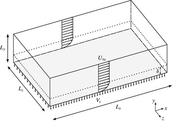
Sketch of the computational domain highlighting the main features of the ASBL flow. The Reynolds number is defined as
 $U_{\infty }/V_{S}$
.

2 Flow case and numerical methodology
2.1 Asymptotic suction boundary layer
The asymptotic suction boundary layer (ASBL) is a boundary-layer flow above a porous flat plate subject to constant homogeneous suction. ‘Asymptotic’ refers to the regime once the flow has developed spatially and reached a constant boundary-layer thickness. In the laminar case the incompressible Navier–Stokes equations admit a steady analytical solution
 $$\begin{eqnarray}u_{L}(y)=U_{\infty }(1-\text{e}^{-yV_{S}/{\it\nu}}),\quad v_{L}=-V_{S},\quad w_{L}=0,\end{eqnarray}$$
which is independent of the streamwise direction (see figure 1). Here
 $(u_{L},v_{L},w_{L})$
is the dimensional laminar velocity field in the streamwise
 $x$
, wall-normal
 $y$
and spanwise
 $z$
directions;
 $U_{\infty }$
and
 $V_{S}>0$
are the free-stream and suction velocities, respectively; and
 ${\it\nu}$
is the kinematic viscosity. The Reynolds number
 $$\begin{eqnarray}Re=\frac{U_{\infty }{\it\delta}^{\ast }}{{\it\nu}}\end{eqnarray}$$
is defined using the displacement boundary-layer thickness
 ${\it\delta}^{\ast }$
of the laminar solution,
 $$\begin{eqnarray}{\it\delta}^{\ast }=\int _{0}^{\infty }\left(1-\frac{u_{L}(y)}{U_{\infty }}\right)\text{d}y.\end{eqnarray}$$
Using expression (2.1) for the laminar solution, equation (2.3) becomes
 ${\it\delta}^{\ast }={\it\nu}/V_{S}$
. Hence
 $Re=U_{\infty }/V_{S}$
is the ratio between the free-stream and suction velocities. The base flow is linearly stable for
 $Re$
up to
 $Re_{c}=54\,370$
(Hocking Reference Hocking1975). However, turbulence can be observed experimentally for values of
 $Re$
much below
 $Re_{c}$
(Antonia et al.
Reference Antonia, Fulachier, Krishnamoorthy, Benabid and Anselmet1988). Sustained turbulence has been reported in recent numerical experiments for
 $Re$
as low as
 $300$
(Schlatter & Örlü Reference Schlatter and Örlü2011; Khapko et al.
Reference Khapko, Duguet, Kreilos, Schlatter, Eckhardt and Henningson2014).
One particular property of the ASBL follows directly from the integral momentum conservation. In both the laminar and turbulent cases the skin friction
 $c_{f}=2(u_{{\it\tau}}/U_{\infty })^{2}$
is fixed once the asymptotic state is reached. This leads to the equilibrium relation
 $$\begin{eqnarray}\left(\frac{u_{{\it\tau}}}{U_{\infty }}\right)^{2}=\frac{1}{Re},\end{eqnarray}$$
where
 $u_{{\it\tau}}$
is the friction velocity. Accordingly, the inner length scale
 $\ell _{\star }={\it\nu}/u_{{\it\tau}}$
used for the viscous scaling reads
 $\ell _{\star }={\it\delta}^{\ast }/\sqrt{Re}$
. The friction Reynolds number is defined as
 $Re_{{\it\tau}}={\it\delta}_{99}u_{{\it\tau}}/{\it\nu}$
or equivalently
 $Re_{{\it\tau}}={\it\delta}_{99}^{+}$
, where
 ${\it\delta}_{99}$
is the
 $99\,\%$
boundary-layer thickness
 $u({\it\delta}_{99})=0.99U_{\infty }$
, and
 $(\cdot )^{+}$
indicates inner scaling.
The laminar displacement thickness
 ${\it\delta}^{\ast }$
together with the free-stream velocity
 $U_{\infty }$
are used as characteristic units for the non-dimensionalisation. From the next section onwards, all quantities are non-dimensional.
2.2 Numerical method
The ASBL is studied numerically using the fully spectral code SIMSON developed at KTH (Chevalier et al.
Reference Chevalier, Schlatter, Lundbladh and Henningson2007). The streamwise and spanwise velocity components are expanded on
 $N_{x}$
and
 $N_{z}$
Fourier modes, respectively, whereas the wall-normal component is expanded using
 $N_{y}$
Chebyshev modes. Dealiasing with the
 $3/2$
rule is performed in the wall-parallel directions. Time stepping is carried out using a third-order Runge–Kutta method for the nonlinear terms and a second-order Crank–Nicolson method for the linear terms. The same numerical method was used in Khapko et al. (Reference Khapko, Kreilos, Schlatter, Duguet, Eckhardt and Henningson2013, Reference Khapko, Duguet, Kreilos, Schlatter, Eckhardt and Henningson2014) to study the dynamics on the laminar–turbulent boundary in ASBL, and by Schlatter & Örlü (Reference Schlatter and Örlü2011) for turbulent ASBL.
The simulations were performed in a cuboid geometry
 ${\it\Omega}=[0,L_{x}]\times [0,L_{y}]\times [0,L_{z}]$
(see figure 1). Periodic boundary conditions are imposed in the wall-parallel directions as a consequence of using a Fourier decomposition. At the lower wall a no-slip condition is imposed. Owing to the finite wall-normal extent of the domain, free-stream boundary conditions are used at
 $y=L_{y}$
. Typically Neumann-type boundary conditions have been used for this purpose in boundary-layer simulations. However, in the case of ASBL, they lead to a slow temporal growth of the boundary layer in the laminar regime (Khapko Reference Khapko2014). Instead, Dirichlet boundary conditions are used here at both lower and upper walls of the domain,
 $$\begin{eqnarray}\displaystyle & \displaystyle (u,v,w)_{y=0}=(0,-1/Re,0), & \displaystyle\end{eqnarray}$$
 $$\begin{eqnarray}\displaystyle & \displaystyle (u,v,w)_{y=L_{y}}=(1,-1/Re,0), & \displaystyle\end{eqnarray}$$
fixing the suction velocity at the upper wall and allowing the correct steady laminar ASBL solution to be captured.
The code is parallelised using both shared and distributed memory parallelisation with the Open Multi-Processing (OpenMP) and Message Passing Interface (MPI), respectively. Two different versions of the MPI parallelisation were used, with domain decomposition in one (
 $z$
) and two (
 $xz$
) directions.
2.3 Study protocol
There are two practical approaches to estimate
 $Re_{g}$
, defined as the largest value of
 $Re$
below which turbulence is never sustained. The first one is to trigger turbulence locally and see whether it persists or decays (Bottin et al.
Reference Bottin, Daviaud, Manneville and Dauchot1998; Avila et al.
Reference Avila, Moxey, de Lozar, Avila, Barkley and Hof2011). However, the method is known to overestimate the value of
 $Re_{g}$
, since the results are dependent on the initial condition. Furthermore, it requires statistical analysis based on a large number of realisations. The second method is the adiabatic approach: the control parameter (here
 $Re$
) is decreased slowly, either continuously or in very small steps, starting from a value where the flow is fully turbulent (Prigent Reference Prigent2001; Barkley & Tuckerman Reference Barkley and Tuckerman2005; Moxey & Barkley Reference Moxey and Barkley2010; Philip & Manneville Reference Philip and Manneville2011). This not only allows one to study the turbulent regime on the verge of laminarisation, but also yields a better quantitative estimate for
 $Re_{g}$
. In our study we have chosen the adiabatic protocol, and proceeded by lowering
 $Re$
from a fully turbulent regime in discrete steps (
 $1.5\,\%$
of the starting value
 $Re=333$
). At each step of the lowering procedure, we wait for the statistically steady regime to be reached (by considering the fluctuating
 ${\it\delta}_{99}$
). Statistics of the flow are then gathered over at least
 $1.6\times 10^{5}$
convective time units, after which the Reynolds number is decreased further. Technically,
 $Re$
is decreased by increasing the suction velocity
 $V_{S}$
, while the free-stream velocity
 $U_{\infty }$
and viscosity
 ${\it\nu}$
are kept constant. This would also be the natural way to proceed in a laboratory experiment, enabling opportunities for future comparison. As
 $Re$
is varied, the value of the laminar displacement thickness
 ${\it\delta}^{\ast }$
changes as well. Therefore, the displacement thickness
 ${\it\delta}_{s}^{\ast }$
at the start value
 $Re=333$
is used as the reference length in the system.
We rely on former numerical studies for an estimation of the initial
 $Re$
to start the adiabatic lowering procedure. Mariani et al. (Reference Mariani, Spalart, Kollmann, So, Speziale and Launder1993) reported sustained turbulence at a value of
 $Re$
as low as
 $278$
(note that they use a different definition for the Reynolds number in their paper). Schlatter & Örlü (Reference Schlatter and Örlü2011) observed sustained turbulence at
 $Re=333$
and laminarisation at
 $Re=280$
starting from a localised perturbation inside the boundary layer. We choose to continue from the latter study, by first obtaining a fully turbulent field at
 $Re=333$
before starting the adiabatic lowering from there.
As discussed in the introduction, the size of the numerical domain plays an important role in correctly capturing the spatio-temporal dynamics of the flow. Moreover, the statistically steady turbulent ASBL becomes independent of the dimensions of the system only for large enough numerical domains (Schlatter & Örlü Reference Schlatter and Örlü2011), with the final
 $99\,\%$
boundary-layer thickness saturating at comparably high values for even moderate
 $Re$
. Using the results of Schlatter & Örlü (Reference Schlatter and Örlü2011) as guidelines, we have chosen the box dimensions to be
 $L_{x}=800$
,
 $L_{z}=400$
and
 $L_{y}=300$
in terms of
 ${\it\delta}_{s}^{\ast }$
(
 ${\it\delta}^{\ast }$
at
 $Re=333$
), with the domain becoming even larger in units of
 ${\it\delta}^{\ast }(Re)$
as
 $Re$
is lowered. Since in most planar shear flows turbulent regions at the onset tend to organise in the form of oblique bands, this computational box was estimated sufficient to fit at least one band, assuming that the band has the same wavelength in inner units as for plane Couette flow. As
 $Re$
is gradually reduced, the
 $99\,\%$
boundary-layer thickness also decreases. Therefore the domain height
 $L_{y}$
was safely reduced for the lowest values of
 $Re$
. The change of grid is performed technically by using spectral interpolation with the Clenshaw recursive algorithm.
Since the value of
 $Re_{g}$
and the observation times required to reach statistically steady regimes at each value of
 $Re$
are not known in advance, preliminary runs using relatively low resolution have been performed first. We used
 ${\rm\Delta}x^{+}\approx 60$
and
 ${\rm\Delta}z^{+}\approx 30$
, which amounts to
 $N_{x}\times N_{y}\times N_{z}=256\times 201\times 256$
spectral modes (case R1 in table 1). Other related under-resolved studies (Willis & Kerswell Reference Willis and Kerswell2009; Manneville & Rolland Reference Manneville and Rolland2011) have pointed out how lower resolution affects the flow quantitatively, mainly by shifting the value of
 $Re_{g}$
, whereas the qualitative comparison with experiments and higher-accuracy numerics remains good. Note that the numerical simulations performed here do not involve any subgrid-scale modelling. These simulations are used in an exploratory manner in order to obtain a rough estimate of
 $Re_{g}$
and, more importantly, to generate turbulent fields close to
 $Re_{g}$
. The lowest values of
 $Re$
are re-examined using higher resolution, with
 ${\rm\Delta}x^{+}\approx 15$
and
 ${\rm\Delta}z^{+}\approx 7.5$
, and a lower value for
 $L_{y}$
(case R2 in table 1).
3 Adiabatic protocol
3.1 Exploratory runs
As mentioned in the previous section, the literature gives only a rough estimate of the value of the critical Reynolds number
 $Re_{g}$
. Initial explorations were performed using the low R1 resolution.
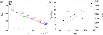
The adiabatic protocol results for the exploratory R1 case. (a) Time evolution of the
 $99\,\%$
boundary-layer thickness
 ${\it\delta}_{99}$
in the stationary regime. Time
 $t$
is scaled with
 ${\it\delta}_{s}^{\ast }/U_{\infty }$
. The Reynolds number was first lowered from
 $Re=333$
down to
 $Re=315$
and from there on in steps of
 $5$
. (b) The corresponding time-averaged values of
 ${\it\delta}_{99}$
(filled circles) scaled with the laminar
 ${\it\delta}_{99L}$
at each
 $Re$
value and
 $Re_{{\it\tau}}={\it\delta}_{99}^{+}$
(open squares, axis to the right) versus
 $Re$
. For the values of
 $Re<Re_{g}$
where the flow is always laminar
 ${\it\delta}_{99}/{\it\delta}_{99L}\equiv 1$
, the value marked with the dashed line.

Simulations performed using different resolutions and domain heights.

We begin the protocol by focusing on the turbulent regime at a fixed value of
 $Re$
, which is then used for the adiabatic lowering. The fully stationary turbulent state is obtained by perturbing the laminar base flow with a localised finite-amplitude disturbance at
 $Re=333$
. In the asymptotic turbulent regime, the
 $99\,\%$
boundary-layer thickness
 ${\it\delta}_{99}$
equilibrates around the value of
 $155$
(see figure 2
a). This value is relatively high compared to the one in the laminar state,
 ${\it\delta}_{99L}\approx 4.6$
, as mentioned in Schlatter & Örlü (Reference Schlatter and Örlü2011) and Bobke et al. (Reference Bobke, Örlü and Schlatter2015), and corresponds to the friction Reynolds number
 $Re_{{\it\tau}}\approx 2800$
(see figure 2
b), reflecting the scale separation in the asymptotic turbulent flow. Recall that
 $Re_{{\it\tau}}$
, sometimes called the Kármán number, expresses the ratio between the largest scales of the boundary layer and the inner scale
 $\ell _{\star }$
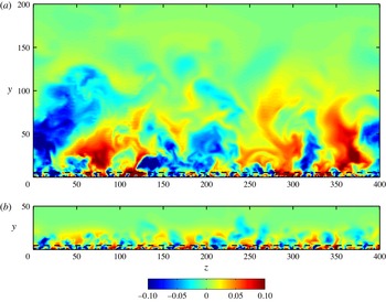
. From figure 3(a) it is evident that several scales coexist within the same flow, with the large-scale structures extending far beyond the near-wall region. This figure is consistent with the attached-eddy hypothesis of Townsend (Reference Townsend1956). The large-scale structures have an influence on the near-wall region, leaving an energy footprint near the wall and modulating the small-scale fluctuations (Bobke et al.
Reference Bobke, Örlü and Schlatter2015), a phenomenon now known as amplitude modulation. This term was coined in Mathis, Hutchins & Marusic (Reference Mathis, Hutchins and Marusic2009), who have investigated the large-scale flow influence in the case of a spatially growing turbulent boundary layer. In their study
 $Re_{{\it\tau}}=2800$
was the lower limit, with the modulation effect getting stronger with increasing
 $Re_{{\it\tau}}$
, as the superstructures also increase in both size and energy.
Two-dimensional
 $yz$
plane visualisations of the streamwise velocity fluctuations
 $u^{\prime }$
at (a)
 $Re=333$
and (b)
 $Re=260$
computed using R1 resolution. Only part of the wall-normal extent of the domain is shown. The black dashed line marks the height
 $y^{+}=100$
. The values of the time-averaged 99 % boundary-layer thickness are
 ${\it\delta}_{99}\approx 155$
and
 $27$
for
 $Re=333$
and
 $260$
, respectively.

The lowering procedure is now described in detail. At the first step, the Reynolds number is decreased from
 $Re=333$
down to
 $Re=315$
, and from there on in intervals of
 $5$
in
 $Re$
. For each value of
 $Re$
, the total simulation time is at least
 $2\times 10^{5}$
convective time units
 ${\it\delta}_{s}^{\ast }/U_{\infty }$
in order to ensure stationarity, with the transients not exceeding
 $0.4\times 10^{5}$
convective units. In figure 2(a) the time evolution of
 ${\it\delta}_{99}$
is shown for the statistically steady part without the transients. The equilibrium value of
 ${\it\delta}_{99}$
decreases monotonically with
 $Re$
. During the step from
 $Re=260$
to
 $Re=255$
, the flow eventually laminarises completely. This gives the guiding value of
 $Re_{g}\approx 260$
that can be used for the high-resolution runs R2, with smaller steps in
 $Re$
deemed unnecessary for the R1 case.
Note that, close to the threshold, the obtained value of
 $Re_{{\it\tau}}=500$
is relatively large. For comparison,
 $Re_{{\it\tau}}$
close to the onset is approximately 60–80 (Tsukahara et al.
Reference Tsukahara, Seki, Kawamura and Tochio2005) for plane Poiseuille flow and approximately 30–50 (Brethouwer et al.
Reference Brethouwer, Duguet and Schlatter2012) for plane Couette flow (based on the half-height between the walls
 $h$
). The latter values are consistent with the estimate for the minimal value of
 $Re_{{\it\tau}}\approx 50$
required for the self-regeneration of turbulent structures in planar shear flows (Waleffe Reference Waleffe1997; Alfredsson & Matsubara Reference Alfredsson and Matsubara2000). In the case of a spatially developing turbulent boundary layer, a value of
 $Re_{{\it\tau}}=140$
was reported close to the inflow by Schlatter & Örlü (Reference Schlatter and Örlü2010a
) (based on the 99 % boundary-layer thickness
 ${\it\delta}_{99}$
). In ASBL the large-scale structures diminish in size with decreasing
 $Re$
; however, the multi-scale nature of the flow remains down to
 $Re_{g}$
, as attested by the large value of the Kármán number
 $Re_{{\it\tau}}$
. This is also evident from figure 3(b), where structures of different scales can be seen, especially comparing the regions below and above the
 $y^{+}=100$
line.
3.2 Identification of partial collapse
As for the laminar–turbulent coexistence, unlike in other wall-bounded shear flows, no laminar regions have been identified visually close to the onset. For instance, at
 $Re=260$
, which is only slightly above
 $Re_{g}$
for the R1 case, turbulence occupies the complete spanwise extent, as evident from figure 3(b). For a more quantitative check, the local wall-shear stress in the spanwise direction
 ${\it\tau}_{z}=|\partial w/\partial y|_{y=0}$
is analysed. This quantity, monitored at an unambiguous wall-normal location, has shown a good indicator of turbulent activity (Kreilos et al.
Reference Kreilos, Khapko, Schlatter, Duguet, Henningson and Eckhardt2016). For the sake of laminar–turbulent distinction, we need to define the smallest elementary cell that can unambiguously be in one of the two states, either laminar or turbulent. Following the ideas of Manneville (Reference Manneville2009), such an elementary cell should have a size comparable with the minimal flow unit (Jiménez & Moin Reference Jiménez and Moin1991), and we have chosen here
 $\text{d}x^{+}\times \text{d}z^{+}\approx 120\times 120$
(that is,
 $\text{d}x\times \text{d}z\approx 6.5\times 6.5$
). The average of
 ${\it\tau}_{z}$
computed over one such cell
 $[{\it\tau}_{z}]\equiv \langle {\it\tau}_{z}\rangle _{cell}$
enables a clear distinction between laminar/quasi-laminar flow and turbulence. While
 $[{\it\tau}_{z}]\approx 0$
in the laminar or quasi-laminar case,
 $[{\it\tau}_{z}]>0$
applies for turbulent flow. Thus, the probability density function (p.d.f.) of
 $[{\it\tau}_{z}]$
computed over the minimal cells in the case of laminar–turbulent coexistence is expected to feature two clear peaks: one close to zero for laminar/quasi-laminar flow, and another one away from zero for turbulence. The local minimum between the two would define the value of the threshold
 $[{\it\tau}_{z}]^{c}$
that would best separate laminar and turbulent values (for more details, see Kreilos et al. (Reference Kreilos, Khapko, Schlatter, Duguet, Henningson and Eckhardt2016)).
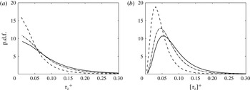
The p.d.f.s of (a) the local wall-shear stress in the spanwise direction
 ${\it\tau}_{z}$
and (b)
 ${\it\tau}_{z}$
averaged over elementary cells
 $[{\it\tau}_{z}]$
capturing independent laminar/turbulent activity for
 $Re=333$
(solid),
 $Re=295$
(dot-dashed) and
 $Re=260$
(dashed), scaled in inner units. The elementary cell size is
 $\text{d}x^{+}\approx 120$
and
 $\text{d}z^{+}\approx 120$
.

In figure 4(a) the p.d.f. of
 ${\it\tau}_{z}$
scaled in inner units is shown. Since the p.d.f. of
 $\partial w/\partial y|_{y=0}$
is symmetric with the mean at zero,
 ${\it\tau}_{z}=|\partial w/\partial y|_{y=0}$
also features a clear peak at zero for all
 $Re$
. But, as mentioned in the previous paragraph, for the purpose of laminar/turbulent discrimination, the data need to be coarse-grained at the level of the minimal cells capturing independent laminar/turbulent activity. The p.d.f. of the coarsened data
 $[{\it\tau}_{z}]$
is shown in figure 4(b). The peak away from zero for all
 $Re$
corresponds to the most probable turbulent value. The probability for a cell to be laminar (
 $[{\it\tau}_{z}]$
being close to 0) increases with decreasing
 $Re$
, but remains low for all values of
 $Re$
. Hence, the flow is fully turbulent even close to the onset, without featuring any extended laminar holes. This behaviour persists when the size of the coarse-graining is varied. Moreover, as the p.d.f.s for different values of
 $Re$
look only self-similar without being superimposable, the increase of the zero-value probability might be attributed to the inner scaling becoming not fully appropriate at low
 $Re$
. The inner scaling is known not to perform well near the onset of sustained turbulence (Ching, Djenidi & Antonia Reference Ching, Djenidi, Antonia, Adrian, Durão, Durst, Heitor, Maeda and Whitelaw1996). In other words, the data at hand do not yield any clear value of
 $[{\it\tau}_{z}]^{c}$
to discriminate between laminar and turbulent, irrespective of the scaling used. The interpretation is that there exists no proper laminar subregion in this flow, i.e. no local turbulence collapse. Note however that the global collapse is easily detectable by monitoring the total kinetic energy of the fluctuations.
3.3 High-resolution reassessment
Turbulent simulations using the R1 resolution suggest no laminar subdomain. This intriguing result has been later verified using high-resolution computations. From here onwards, all the results presented are obtained using the finer R2 resolution.
The velocity fields obtained using the R1 resolution serve as the initial conditions for the R2 case at the same value of
 $Re$
. The resolution is then increased by steps in all directions until the desired R2 accuracy is reached. This approach avoids repeating the costly lowering procedure and to immediately focus on the most interesting range where
 $Re\gtrsim Re_{g}$
. With this method the critical Reynolds number is found to be
 $Re_{g}=270$
. Turbulence collapses globally every time
 $Re$
is decreased from 270 to 269 or lower, independent of the initial condition. Thus, the resolution improvement from R1 to R2 corresponds to a shift of approximately 10 in
 $Re_{g}$
, i.e. less than 4 %. This agrees well with the results of Manneville & Rolland (Reference Manneville and Rolland2011), who documented a similar trend – under-resolved simulations lead to a down-shift of the transitional range in terms of
 $Re$
.
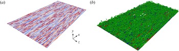
A snapshot of the turbulent regime at
 $Re=270$
is shown in figure 5. The
 $xz$
plane close to the wall at
 $y^{+}\approx 12$
(figure 5
a) reveals that the whole near-wall region is filled with streaks. Some of these streaks are in the bursting phase, recognised in figure 5(a) by small-scale fluctuations distorting the elongated streaky structures, while others are in a calm phase at the considered time instant, but bursting at another time. Figure 5(b) shows isolevels of the vortex criterion
 ${\it\lambda}_{2}$
(Jeong & Hussain Reference Jeong and Hussain1995). A uniformly dense forest of vortices is present not only near the wall but also extending away from it. From figure 5 it is evident there are no clear laminar holes close to
 $Re_{g}$
. This confirms the conclusions drawn from the wall-shear stress (figure 4
b). High-accuracy computations improve the estimation of
 $Re_{g}$
, but qualitatively display the same features as in the R1 case. In particular, neither STI nor patterning has been detected near the onset.
Three-dimensional visualisation of the well-resolved flow field (resolution R2) at
 $Re=270$
. (a) The
 $xz$
plane at
 $y^{+}\approx 12$
with positive (red) and negative (blue) streamwise velocity fluctuations (values range between
 $u^{\prime +}=\pm 2.46$
). (b) Isosurfaces of the streamwise velocity fluctuations
 $u^{\prime +}=\pm 1.15$
(red and blue) and
 ${\it\lambda}_{2}$
criterion
 ${\it\lambda}_{2}^{+}=-5\times 10^{-5}$
(green). Flow is from lower left to upper right.

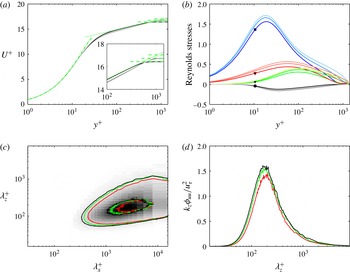
Statistical quantities for the well-resolved case. (a) Mean streamwise velocity profiles for
 $Re=270$
,
 $Re=280$
and
 $Re=290$
, with the lighter colours corresponding to increasing
 $Re$
. The green dot-dashed line corresponds to the modified linear law (Simpson Reference Simpson1967). The green dotted line represents the empirical log law
 $u^{+}=(1/{\it\kappa})\ln y^{+}+B$
for
 $Re=270$
with
 ${\it\kappa}=1.1$
and
 $B=10.7$
. The free-stream velocity in inner scaling
 $U_{\infty }^{+}$
is marked with the green dashed lines. (b) Reynolds stresses:
 $u_{\mathit{rms}}$
(marked with a square),
 $v_{\mathit{rms}}$
(star),
 $w_{\mathit{rms}}$
(triangle) and
 $\overline{u^{\prime }v^{\prime }}$
(circle) at
 $Re=270$
, and lighter colours for increasing
 $Re$
, i.e.
 $Re=280$
and
 $Re=290$
. (c) Two-dimensional premultiplied energy spectrum
 ${\it\phi}_{uu}^{+}({\it\lambda}_{x}^{+},{\it\lambda}_{z}^{+})$
at position
 $y^{+}=12$
for
 $Re=270$
(red solid line),
 $Re=280$
(green solid line) and
 $Re=290$
(black solid line). Contour lines correspond to
 $0.08$
and
 $0.6$
of the maximum value at
 $Re=290$
and pseudocolours of the spectrum at
 $Re=290$
are shown in the background. (d) One-dimensional premultiplied energy spectrum
 ${\it\phi}_{uu}^{+}({\it\lambda}_{z}^{+})$
at
 $y^{+}=12$
with the same colour scheme as in panel (c).

After confirming the space-filling nature of the turbulent regime near the onset, the usual turbulence statistics can be computed in order to shed further light on the structure of the flow. Selected results are reported in figure 6: the mean streamwise velocity profiles (figure 6
a) feature a distinct log layer, with the overall shape being comparable with higher-
 $Re$
statistics (Schlatter & Örlü Reference Schlatter and Örlü2011). A feature of the asymptotic turbulent regime is the absence of a clear wake region, as opposed to the untranspired zero-pressure-gradient turbulent boundary layer. This confirms that the appropriate size requirements are satisfied. The modified linear law, derived for the cases with transpiration (Simpson Reference Simpson1967), provides good agreement very close to the wall for all suction rates. Inside the logarithmic region the empirical log law
 $u^{+}=(1/{\it\kappa})\ln y^{+}+B$
is fitted to the
 $Re=270$
profile with
 ${\it\kappa}=1.1$
and
 $B=10.7$
, i.e. different from the canonical boundary layers. The parameters
 ${\it\kappa}$
and
 $B$
are
 $Re$
-dependent and increase here with decreasing
 $Re$
. The same trend was observed at much higher
 $Re$
by Bobke et al. (Reference Bobke, Örlü and Schlatter2015). In figure 6(b) the Reynolds stresses are shown. Applying suction decreases all stresses compared to the spatially developing boundary layer. The reduction gets more pronounced with decreasing
 $Re$
. This trend is seen both in figure 6(b) and in the works of Mariani et al. (Reference Mariani, Spalart, Kollmann, So, Speziale and Launder1993) and Schlatter & Örlü (Reference Schlatter and Örlü2011).
Furthermore, the two-dimensional premultiplied spectrum of the streamwise velocity fluctuations, defined as
 ${\it\phi}_{uu}^{+}({\it\lambda}_{x},{\it\lambda}_{z})=k_{x}k_{z}{\it\phi}_{uu}({\it\lambda}_{x},{\it\lambda}_{z})/u_{{\it\tau}}^{2}$
, is considered inside the buffer layer (see figure 6
c). The peak near
 ${\it\lambda}_{x}^{+}=10^{3}$
and
 ${\it\lambda}_{z}^{+}=10^{2}$
captures the near-wall streamwise streaks. This peak shifts slightly towards wider scales with decreasing
 $Re$
. The one-dimensional spanwise premultiplied spectrum
 ${\it\phi}_{uu}^{+}({\it\lambda}_{z})=k_{z}{\it\phi}_{uu}({\it\lambda}_{z})/u_{{\it\tau}}^{2}$
is shown in figure 6(d). The peak is located at
 ${\it\lambda}_{z}^{+}\approx 150$
and varies only weakly with
 $Re$
. As noted before by Schlatter & Örlü (Reference Schlatter and Örlü2011) and Bobke et al. (Reference Bobke, Örlü and Schlatter2015), the streaks in turbulent ASBL are slightly wider compared to the case without suction. These data confirm that turbulence is sustained without intermittency down to the lowest
 $Re$
before global collapse.
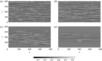
Two-dimensional
 $xz$
plane visualisations demonstrating the flow on its way to laminarisation when the Reynolds number is decreased from
 $Re=270$
down to
 $Re=269$
. The streamwise velocity
 $u$
at
 $y^{+}\approx 12$
is shown at times (a)
 $t=0$
, (b)
 $t\approx 1.38\times 10^{4}$
, (c)
 $t\approx 1.7\times 10^{4}$
and (d)
 $t\approx 3\times 10^{4}$
.

3.4 Global collapse of turbulence
Up to this point, no steady or even transient laminar–turbulent coexistence has been observed in ASBL. Therefore, it is only when the turbulence collapses globally that clear laminar regions emerge. By definition, when the flow is adiabatically lowered below
 $Re_{g}$
, global collapse of turbulence eventually occurs with unit probability. Beyond the quantitative value of
 $Re_{g}$
, the analysis of the laminarisation process itself is rich in information.
The current focus is on cases where
 $Re$
is reduced from
 $Re>Re_{g}$
to
 $Re\lesssim Re_{g}$
. A robust sequence of events leading to laminarisation of the flow is observed in all cases; hence it is enough to scrutinise one such case to identify the generic features of the laminarisation process in ASBL. A global collapse event occurring when lowering
 $Re$
from
 $270$
to
 $269$
is chosen for this purpose.
The whole process is shown using a sequence of snapshots of
 $u(x,y^{+}=12,z)$
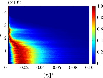
displayed in figure 7. In addition, the evolution of the p.d.f. of
 $[{\it\tau}_{z}]$
is shown in figure 8. When the flow is fully laminar, the p.d.f. peaks at zero. Thus, in order to be able to compare the p.d.f.s in turbulent and laminar flow, normalisation with the local maximum is used. Unlike figure 4(b), the p.d.f. in figure 8 is obtained by averaging over only a few consecutive snapshots. Consequently, the data in figure 8 appear more noisy, but clearly highlight the difference between the laminar and turbulent regimes.
Time evolution of the probability density function of
 $[{\it\tau}_{z}]$
computed using the same size of elementary cells as in figure 4(b). The Reynolds number is lowered from
 $Re=270$
to
 $Re=269$
. The values of the p.d.f. are rescaled with the maximum at each time instant.

The initial time (
 $t=0$
) corresponds to the fully turbulent regime at
 $Re=270$
(figure 7
a). The p.d.f. of
 $[{\it\tau}_{z}]$
features a clear zero probability for
 $[{\it\tau}_{z}]=0$
, confirming again the absence of laminar holes. As the flow adapts to the new value of
 $Re$
, the most probable values of
 $[{\it\tau}_{z}]$
shift towards zero. At the same time, spatial regions with reduced fluctuations appear at the top and bottom in figure 7(b). This weakening of the turbulent activity ultimately leads to partial laminarisation of the flow. At
 $t\approx 1.7\times 10^{4}$
, the first laminar holes form (see figure 7
c). At this point in figure 8 a non-zero probability is attained at
 $[{\it\tau}_{z}]=0$
, which then grows with the expansion of the laminar holes. As the weaker turbulence regions from figure 7(b) laminarise they also spread fast in the streamwise direction until their length reaches
 $L_{x}$
. This seems to be a general feature of ASBL, as the formation of laminar holes predominantly happens through elongation in the streamwise direction. This leads to a state featuring turbulent and laminar bands, both aligned with the streamwise direction. The fluctuations in the turbulent zones progressively weaken, until these further break up into turbulent patches (see figure 7
d). These patches do not spread at this value of
 $Re$
and all eventually decay between
 $t\approx 3\times 10^{4}$
and
 $t\approx 4\times 10^{4}$
.
In summary, the whole collapse process can be split into two phases. During the first one, the laminar holes appear and grow to form streamwise laminar avenues. Next, the turbulence activity in the streamwise bands diminishes, and they laminarise through the (dis)appearance of transient turbulent spots.
This phenomenon differs from the collapse process reported, for example, in plane Couette and plane Poiseuille flows. There, laminar–turbulent bands are oblique with respect to the
 $x$
direction and persist for a long time. Once a hole spontaneously forms inside one turbulent band, turbulence retracts in the direction of the band (Manneville Reference Manneville2011). In ASBL no robust oblique interface separating laminar from turbulent regions has been detected; instead, only streamwise-elongated interfaces. Since in the other planar shear flows the large-scale flow is held responsible for the obliqueness of interfaces, any explanation for the peculiarity of ASBL has to incorporate the notion of large-scale flow as well.
3.5 Hypothesis about the role of the large-scale flow
A distinctive feature of turbulent ASBL is the clear scale separation that remains down to the lowest
 $Re$
with sustained turbulence. The explanation lies in the fact that the large-scale fluctuations in the wall-normal direction, i.e. ejections and sweeps, may appear at relatively low
 $Re$
. These events lead to the creation of a large-scale flow (LSF) away from the wall. In order to understand the difference between the LSF at the onset in ASBL and in the wall-bounded internal shear flows, we elaborate on the ideas of Duguet & Schlatter (Reference Duguet and Schlatter2013). Consider the continuity equation valid at any location
 $$\begin{eqnarray}\partial _{x}u+\partial _{y}v+\partial _{z}w=0.\end{eqnarray}$$
Applying large-scale spatial filtering to (3.1) leads to
 $$\begin{eqnarray}\partial _{x}U+\partial _{y}V+\partial _{z}W=0,\end{eqnarray}$$
where large-scale components are denoted with the upper case. The cutoff wavelength should be chosen larger than the average size of the near-wall structures.
Integrating (3.2) from the wall, here located at
 $y=0$
, to some arbitrary value
 $y=l$
yields
 $$\begin{eqnarray}\partial _{x}\bar{U}+\overline{\partial _{y}V}+\partial _{z}\bar{W}=0,\end{eqnarray}$$
where the overbar denotes wall-normal integration, i.e.
 $\bar{(\cdot )}=\int _{0}^{l}(\cdot )\,\text{d}y$
. Performing the integration of the wall-normal term leads to
 $$\begin{eqnarray}\partial _{x}\bar{U}+\partial _{z}\bar{W}=V(0)-V(l).\end{eqnarray}$$
For plane Couette and plane Poiseuille flow close to
 $Re_{g}$
, the near-wall structures actually scale with the gap width
 $2h$
. In that case, the walls are impermeable, and
 $y$
-averaging performed between the two walls in (3.4) leads to
 $$\begin{eqnarray}\partial _{x}\bar{U}+\partial _{z}\bar{W}=0.\end{eqnarray}$$
The
 $y$
-integrated LSF in such a case is hence two-dimensional and divergence-free in the plane. Duguet & Schlatter (Reference Duguet and Schlatter2013) have suggested that the transport of weak fluctuations by this flow close to a laminar–turbulent interface should result in an oblique stripe in the
 $xz$
plane, precisely because
 $(\bar{U},\bar{W})$
displays obliqueness due to the streamwise deceleration at the laminar–turbulent interfaces.
In ASBL, wall-normal integration between 0 and any finite
 $l$
leads to
 $$\begin{eqnarray}\partial _{x}\bar{U}+\partial _{z}\bar{W}=-V_{S}-V(l).\end{eqnarray}$$
For
 $l$
inside the boundary layer, there are large eddies, typically large-scale sweeps and ejections; hence the term
 $V(l)$
is not equal to
 $-V_{S}$
, resulting in a non-vanishing right-hand side in (3.6). Thus, even if
 $\partial _{x}\bar{U}$
is different from zero (for instance, near a laminar–turbulent interface), (3.5) does not hold. However, the obliqueness of laminar–turbulent interfaces is closely connected to (3.5). This suggests that fully oblique laminar–turbulent interfaces are not generically expected in ASBL, even in the case of growing turbulent spots. This hypothesis can actually be tested numerically by manipulating the LSF of ASBL so that it becomes nearly two-dimensional, as in plane Couette or plane Poiseuille flow. In the next section we will show the effects of suppressing the flow in the outer region of the boundary layer.
4 Manipulation of the outer flow
There are several ways to manipulate the flow in order to prevent large-scale structures from forming away from the wall. One physical way is to use stable density stratification, which directly damps all wall-normal turbulent motion and in turn distorts the LSF. In Ekman boundary-layer flows, the addition of strong stable stratification leads to the formation of laminar–turbulent bands near the wall (Deusebio et al. Reference Deusebio, Brethouwer, Schlatter and Lindborg2014). However, applying stratification to ASBL might be difficult to interpret, as it is not clear which effect, suction, stratification or the weaker outer-layer motions, will be dominant.
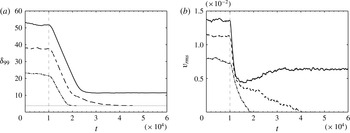
Time evolution of integral quantities before and after applying the forcing at time
 $t=1\times 10^{4}$
(marked with the dashed line). (a) Boundary-layer thickness
 ${\it\delta}_{99}$
. The laminar value for
 $Re=270$
is marked with the dotted line. (b) Root-mean-square value of the wall-normal velocity fluctuations
 $v_{rms}$
. The Reynolds numbers shown are
 $Re=270$
(dot-dashed),
 $Re=280$
(dashed) and
 $Re=290$
(solid).

Another possibility to damp the LSF, linked more to the hierarchy of scales, is to restrict the size of the largest structures accommodated by the flow. This can be achieved by explicitly removing all fluctuations above a certain distance away from the wall. Jiménez & Pinelli (Reference Jiménez and Pinelli1999) used this method in order to test and remove the influence of the outer flow on the near-wall regeneration cycle. Besides restricting the largest possible scales using geometrical constraints imposed by the boundary conditions, they also solved the Navier–Stokes equations with the addition of a dissipative body force damping all the fluctuations above a fixed
 $y$
location. Their results have shown that the region below
 $y^{+}=60$
is autonomous and preserves all the necessary ingredients of the near-wall cycle. A similar approach is chosen in this study. A volume forcing is added, suppressing all spanwise and wall-normal fluctuations above a fixed distance from the wall. This sets an upper limit to the wall-normal extent of the large-scale wall-normal and spanwise motion and consequently damps the outer flow. However, compared to the work of Jiménez & Pinelli (Reference Jiménez and Pinelli1999), the present use of a spatially extended numerical domain would permit spanwise-extended but vertically constrained structures.
The forcing is added on the right-hand side of the Navier–Stokes equations in the form
 $\boldsymbol{F}=(0,{\it\lambda}(y)(-V_{S}-v),{\it\lambda}(y)(-w))$
. Here
 ${\it\lambda}(y)$
is the fringe function, and
 $v$
and
 $w$
are the current wall-normal and spanwise velocity components with the desired values above the fringe
 $-V_{S}$
and
 $0$
, respectively. Since a priori the streamwise velocity profile above the fringe is not known, only the wall-normal and spanwise components of the velocity fluctuations are relaxed towards the basic state. This in turn leads to the viscous decay of the streamwise component
 $u$
. The fringe function
 ${\it\lambda}(y)=S((y-y_{s})/d)$
takes the form of the step function
 $S(u)$
defined in Chevalier et al. (Reference Chevalier, Schlatter, Lundbladh and Henningson2007) as
 $$\begin{eqnarray}S(u)=\left\{\begin{array}{@{}ll@{}}0, & u\leqslant 0,\\ 1/(1+\text{e}^{(1/(u-1)+1/u)}), & 0<u<1,\\ 1, & u\geqslant 1.\end{array}\right.\end{eqnarray}$$
This function is zero below the starting position
 $y_{s}$
, then smoothly grows from
 $0$
to
 $1$
in the interval
 $(y_{s},y_{s}+d)$
and stays equal to
 $1$
thereafter. A range of values for the parameters of the forcing were tested, i.e.
 $y_{s}^{+}\in [50,100]$
and
 $d^{+}\in [10,180]$
. Finally, the values
 $y_{s}^{+}=100$
and
 $d^{+}\approx 80$
were chosen as a compromise between effective removal of the LSF and not affecting the near-wall dynamics.
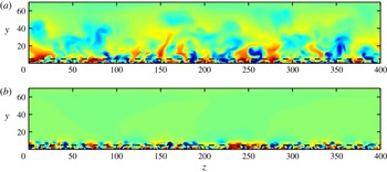
Two-dimensional
 $yz$
plane visualisations of the streamwise velocity fluctuations at
 $Re=290$
(a) before and (b) after applying the forcing. The black dashed line marks the height
 $y^{+}=100$
. The colour map is the same as in figure 3. The values of the time-averaged 99 % boundary-layer thickness are
 ${\it\delta}_{99}\approx 52$
and
 $11$
before and after the forcing is applied, respectively.

Three cases are considered:
 $Re=270$
,
 $Re=280$
and
 $Re=290$
. The time evolution of
 ${\it\delta}_{99}$
and
 $v_{rms}$
is shown in figure 9. In order not to shock the flow, which can lead to accidental laminarisation, the strength of the damping is smoothly increased from
 $0$
to
 $1$
starting at time
 $t=1\times 10^{4}$
over a window of
 $2\times 10^{4}$
time units. In two cases,
 $Re=270$
and
 $Re=280$
, turbulence collapses completely. This is indicated by
 ${\it\delta}_{99}$
reaching the laminar values and the strength of the wall-normal fluctuations
 $v_{rms}$
falling down to zero. At
 $Re=290$
, after a transient period where the outer flow is annihilated, the near-wall region of the flow remains turbulent. However, it is now associated with both lower boundary-layer thickness and fluctuation levels compared to the original case without the forcing. The linear decrease of
 ${\it\delta}_{99}$
is due to the viscous decay of the streamwise fluctuations following the direct damping of the wall-normal and spanwise fluctuations.
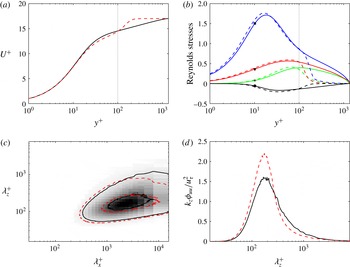
Comparison of statistical quantities for the cases without (solid) and with (dashed) the forcing at
 $Re=290$
. (a) Mean streamwise velocity profile. The wall-normal position
 $y^{+}=100$
is marked with the dotted vertical line. (b) Reynolds stresses:
 $u_{\mathit{rms}}$
(marked with a square),
 $v_{\mathit{rms}}$
(star),
 $w_{\mathit{rms}}$
(triangle) and
 $\overline{u^{\prime }v^{\prime }}$
(circle). (c) Two-dimensional premultiplied energy spectrum
 ${\it\phi}_{uu}^{+}({\it\lambda}_{x}^{+},{\it\lambda}_{z}^{+})$
at position
 $y^{+}=12$
. Contour lines correspond to
 $0.08$
and
 $0.6$
of the maximum value at
 $Re=290$
without the forcing, and pseudocolours of the spectrum at
 $Re=290$
are shown in the background. (d) One-dimensional premultiplied energy spectrum
 ${\it\phi}_{uu}^{+}({\it\lambda}_{z}^{+})$
at
 $y^{+}=12$
.

Laminarisation occurring at
 $Re>Re_{g}$
implies that the forcing interferes with the mechanisms sustaining turbulence in ASBL close to the onset. The starting
 $y$
position of the forcing is well above the limit given by Jiménez & Pinelli (Reference Jiménez and Pinelli1999) necessary for the autonomous near-wall cycle. Hence, the global turbulence collapse at
 $Re=270$
and
 $Re=280$
suggests that the large-scale structures away from the wall are an important ingredient of the sustaining mechanism of turbulent ASBL too, and removing them close to
 $Re_{g}$
causes laminarisation. Results obtained for slightly varied parameters of the forcing, e.g. its position, strength or period over which it is smoothly applied, qualitatively support the above conclusion.
The effect of the forcing on the organisation of turbulence in the case it is sustained (
 $Re=290$
) is shown in figure 10. The large-scale motion away from the wall in figure 10(a) is effectively suppressed in figure 10(b). Still, turbulence covers the whole spanwise extent without apparent laminar holes, i.e. no persistent laminar bands appear. Comparison of turbulent statistics before and after applying the forcing is presented in figure 11. The logarithmic region (roughly
 $10^{2}<y^{+}<10^{3}$
) of the streamwise velocity profile (figure 11
a) nearly vanishes in the latter case. The inner linear part of the profile is now almost immediately connected to the free stream through a distinct wake region. Such a distinct wake region also appears in the turbulent ASBL profile when the numerical domain size is reduced beyond a specific limit (Bobke et al.
Reference Bobke, Örlü and Schlatter2015). Hence the effects of wall-normal forcing and restricted domain size on the turbulent flow are similar. They both prevent the large-scale structures from forming, which in turn alters the profile in the outer region. The mechanism of the damping is well illustrated by the Reynolds stresses shown in figure 11(b). Both wall-normal and spanwise components quickly attain zero values above
 $y^{+}=100$
, but there is no sharp discontinuous drop due to the appropriate smoothing. The streamwise component is not directly manipulated, so its decay starts slightly higher than the
 $y^{+}=100$
position. Figure 11(a,b) shows that the near-wall region is left fairly intact by the action of the damping. The weak discrepancy between Reynolds stresses below
 $y^{+}=100$
, before and after the forcing is applied, indicates that it has a limited influence on the inner scaling, or more precisely on the friction velocity
 $u_{{\it\tau}}$
. Indeed, the agreement is seen to improve when
 $u_{{\it\tau}}$
is changed by approximately
 $4\,\%$
.
The two-dimensional premultiplied energy spectrum
 ${\it\phi}_{uu}^{+}({\it\lambda}_{x}^{+},{\it\lambda}_{z}^{+})$
in figure 11(c) reveals that the most energetic structures near the wall remain approximately of the same size, before and after applying the forcing. However, there is a clear drop-off in energy corresponding to the larger scales (both streamwise and spanwise). Moreover, as seen in figure 11(d), while the energy content of the largest spanwise scales is decreasing, the near-wall streaks become slightly more energetic with the forcing turned on, possibly due to the restricted energy transfer to larger scales.
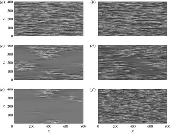
Two-dimensional
 $xz$
plane visualisations demonstrating the influence of the wall-normal damping on the flow at Reynolds numbers
 $Re=280$
(a,c,e) and
 $Re=290$
(b,d,f). The streamwise velocity at
 $y^{+}\approx 12$
is shown at times (a)
 $t\approx 1\times 10^{4}$
, (c)
 $t\approx 2.1\times 10^{4}$
and (e)
 $t\approx 3\times 10^{4}$
for
 $Re=280$
, and at (b)
 $t\approx 1\times 10^{4}$
, (d)
 $t\approx 1.8\times 10^{4}$
and (f)
 $t\approx 4.3\times 10^{4}$
for
 $Re=290$
. The colour map is the same as in figure 7.

Yet the most interesting effect of the forcing is seen during the transient phase before fully laminar or turbulent flow is established. The snapshots of the near-wall
 $xz$
planes demonstrating the two cases,
 $Re=280$
and
 $Re=290$
, are shown in figure 12. At
 $Re=280$
turbulence collapses, but the events leading to the laminar state are very different from the ones described in § 3.4. The two-step process with the laminar avenues followed by transient spots is not observed in this case. Instead, the collapse process is reminiscent of the behaviour reported in other genuinely planar flow cases. Before all turbulent zones decay, the laminar–turbulent interfaces organise obliquely with respect to the streamwise direction (figure 12
c). Furthermore, even in the case when turbulence survives under the effect of the forcing at
 $Re=290$
, transient laminar regions (i.e. holes) appear. They are also oblique, forming a stripe-like structure in the flow (figure 12
d). Loose measurements from figure 12 suggest an angle with the streamwise direction in the range
 ${\approx}10^{\circ }{-}40^{\circ }$
, comparable with the values reported in plane Couette flow (Barkley & Tuckerman Reference Barkley and Tuckerman2005; Duguet et al.
Reference Duguet, Schlatter and Henningson2010). However, turbulence is expanding and filling the wall-parallel extent again.
Hence, by suppressing the outer flow, we were able to probe its effect on the turbulent regime near the onset and on the dynamics of turbulence collapse. Under the effect of the artificial confinement, the flow either laminarises or stays fully turbulent. However, during the transient phase, laminar holes appear, with oblique interfaces. Thus, manipulating the flow and removing the large-scale structures leads to similar laminar–turbulent dynamics as in other wall-bounded shear flows.
5 Discussion and conclusions
We have investigated numerically the asymptotic suction boundary layer (ASBL) at the onset of turbulence in an extended domain using an adiabatic protocol. Starting from a fully turbulent flow, the Reynolds number is lowered until global turbulence collapse occurs. An estimate of the threshold
 $Re_{g}\approx 270\pm 1$
(for the specific observation time) is obtained below which turbulence is not sustained, improving the previous assessments in ASBL.
Surprisingly, the nature of the turbulent regime just above the threshold
 $Re_{g}$
and the sequence of events leading to laminarisation in ASBL strongly differ from wall-bounded internal shear flows, i.e. fully enclosed flows. Whereas there is growing evidence that Poiseuille and Couette flows might undergo continuous phase transitions involving a well-defined critical point (Lemoult et al.
Reference Lemoult, Shi, Avila, Jalikop, Avila and Hof2016; Sano & Tamai Reference Sano and Tamai2016), the present data strongly suggest a fully discontinuous phase transition: the turbulent fraction at equilibrium is either 0 or 100 % but never achieves intermediate values. Even close to
 $Re_{g}$
, turbulence is area-filling, with no evident traces of laminar holes; whereas, in other planar shear flows close to
 $Re_{g}$
, laminar and turbulent regimes coexist in the form of more robust oblique laminar–turbulent patterns. Obviously, such conclusions, especially related to continuity, remain to be tested in larger computational domains and over observation times that are larger by at least one order of magnitude. Typical laminarisation events observed in the current investigation of ASBL can be split into two stages. In the first one, turbulence partially collapses, creating laminar holes, which quickly grow into long streamwise laminar avenues. After this, the remaining turbulent zones separate into individual spots, which eventually decay. In wall-bounded internal shear flows, a slow decrease of
 $Re$
starting from a laminar–turbulent pattern regime leads to the creation of laminar holes inside the turbulent bands. Consequently, the bands shrink.
The feature that distinguishes ASBL from the other flows, such as plane Couette flow and plane Poiseuille flow, is the large-scale wall-normal transport. It turns out that laminar–turbulent patterns can now, where they occur, be interpreted in a new fashion: as
 $Re$
is reduced in plane Couette flow, the onset
 $Re\approx Re_{g}$
corresponds to wall-normal large scales being indistinguishable from small scales. Wall-normal confinement hence leads to a planar large-scale flow only, making laminar–turbulent patterns sustainable – at least over a range of values of
 $Re$
. In the cases of plane Couette flow with spanwise cyclonic rotation and plane magnetohydrodynamic channel flow, the wall-normal motion is distorted, as the laminar–turbulent bands are confined close to the wall with the core of the flow being turbulent. The same mechanism is at play in the strongly stratified Ekman layer, where stable stratification directly damps the wall-normal motion. In all above-mentioned cases, the large-scale flow takes the form of a secondary flow around turbulent bands and acts parallel to the wall.
In ASBL the large-scale wall-normal transport is never prohibited and leads to creation of large-scale structures which extend far away from the wall. A hierarchy of scales, rather typical of higher-
 $Re$
turbulence, persists even close to
 $Re_{g}$
, which is also expressed in the fact that the inner-scale boundary-layer thickness at
 $Re_{g}$
is approximately
 $490$
. The large-scale flow in ASBL is hence three-dimensional rather than purely planar and takes the form of large-scale structures (typically large-scale streamwise vorticity and streaks) reaching far above the near-wall region. Their influence on the dynamics near the wall can explain the discrepancies of transitional ASBL compared to the other planar shear flows.
By removing all the large-scale structures above the
 $y^{+}=100$
level, we have confirmed their influence on the character of the laminar–turbulent interfaces in ASBL. Suppressing all perturbations in the outer region makes ASBL more similar to the wall-bounded internal shear flows. Consequently, the analysis in Duguet & Schlatter (Reference Duguet and Schlatter2013) and § 3.5 becomes applicable to the manipulated ASBL flow, and oblique laminar–turbulent interfaces are seen to appear, at least transiently. The obliqueness is, however, not sufficient, but only a necessary condition for the laminar–turbulent patterning phenomenon. In other words, removing the large-scale structures is still not sufficient for recovering the same behaviour of other wall-bounded shear flows, namely an equilibrium state with oblique laminar–turbulent patterns. The mechanism responsible for streamwise localisation, i.e. the lack of occurrence of laminar–turbulent bands (or laminar zones in general) in ASBL at the onset remains to be explained. However, the latter might also be connected with the large-scale outer structures present in ASBL at the onset. When these structures are damped, turbulence collapse at some
 $Re>Re_{g}$
is observed. This can indicate the importance of the large-scale flow away from the wall for the self-sustenance of the flow close to
 $Re_{g}$
. The large-scale structures in the outer region, via their transport of turbulent fluctuations, can re-initiate turbulence if it retracts in one of the regions near the wall. This could explain the absence of persistent holes close to
 $Re_{g}$
. Moreover, when the transport by the large scales is not able to re-initiate turbulence, a local collapse event can lead to relaminarisation along the whole streamwise direction: reduction of turbulent fluctuations somewhere in the flow lead to weakening and disappearance of the associated large-scale structures. This in turn leads to partial turbulence collapse in the whole streamwise region below the large-scale structures, creating streamwise laminar avenues. However, this mechanism has to be validated by future studies. In addition, the presence of suction in the immediate near-wall region might influence the dynamics during laminarisation and thus complicate the comparison to non-transpired cases. Why some flows display streamwise localisation, at least for low
 $Re$
, is an important issue that needs to be addressed in a more general context.
This study suggests that strong large-scale wall-normal motions such as outer-layer ejections and sweeps, typical of both parallel and spatially growing boundary layers, are not compatible with sustained oblique laminar–turbulent interfaces.
The appearance of large-scale turbulent structures in most planar shear flows is traditionally associated with large Reynolds numbers. At high
 $Re$
, i.e. also high
 $Re_{{\it\tau}}$
, the scales of the near-wall fluctuations are much smaller than the outer scales prescribed by the geometry of the flow. Consequently, this allows for larger structures to fill the gap between the walls. In plane Poiseuille flow and plane Couette flow, this coexistence of different wall-normal scales is only possible, by definition, for large enough
 $Re_{{\it\tau}}$
, which corresponds to high
 $Re$
(see e.g. Orlandi, Bernardini & Pirozzoli Reference Orlandi, Bernardini and Pirozzoli2015). In the Blasius boundary layer, large outer-layer structures, as well as their modulating influence on smaller scales, are associated with longer time scales. They develop slowly, which translates into spatial locations further downstream, again associated with higher
 $Re$
(Mathis et al.
Reference Mathis, Hutchins and Marusic2009; Schlatter & Örlü Reference Schlatter and Örlü2010b
). ASBL is peculiar in the sense that it is an equilibrium boundary layer and thus the large-scale turbulent structures are present right at the onset of sustained turbulence, i.e. at relatively low
 $Re$
.
The question of the experimental realisability of stationary turbulent ASBL in a wind tunnel of finite length remains open even at low Reynolds number (Bobke et al.
Reference Bobke, Örlü and Schlatter2015), because of the length required in practice to reach such a state. However, the global collapse of turbulence is inevitable below some
 $Re$
. The experimental collapse process from a non-asymptotic turbulent state remains to be compared with the sequence of events described in the present study.
Acknowledgements
Computer time provided by SNIC (Swedish National Infrastructure for Computing) is gratefully acknowledged. Computations were performed at NHPC (Iceland), NSC (Linköping) and PDC (Stockholm).