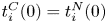
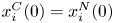
1. Introduction
The literature reveals that environmental R&D cartels with full information sharing – that is, research joint venture cartels – internalize the public goods nature of knowledge generated by technology development and maximize social welfare. However, important international aspects of research joint venture (RJV) cartels, where firms in different countries cooperate on environmental R&D and governments act strategically, remain unanalyzed.
In international contexts under imperfect competition, governments distort environmental policies by acting strategically to obtain rent (Conrad, Reference Conrad1993; Barrett, Reference Barrett1994; Kennedy, Reference Kennedy1994).Footnote 1 Therefore, researchers must consider the effects on strategic environmental policy when evaluating the performance of environmental RJV cartels in international contexts. This paper sheds light on this subject.Footnote 2
We consider a third-country model that features Cournot duopoly. Two firms in different countries cooperate with environmental R&D and governments act strategically. The environmental technology we consider is end-of-pipe. Using this model reveals that three categories of incentives potentially distort environmental policy under R&D/RJV cartels: the rent-shift effect, the over-investment effect, and the environmental spillover effect. That is, governments have incentives to set lower environmental tax rates to obtain rents; to set lower tax rates to remedy ‘over-investment by firms’; and to set higher tax rates to promote investment by rivals.
If the over-investment effect dominates, environmental taxation under an R&D/RJV cartel is below that under R&D/RJV competition, reducing rent extraction from consumers in the third county. Contrary to conventional wisdom, an RJV cartel cannot engender maximum social welfare, but RJV cartels work well for environmental investment.
In addition, promoting an R&D/RJV cartel could diminish consumer surplus in the third country if environmental tax under an R&D/RJV cartel exceeds that under R&D/RJV competition. Therefore, promoting an R&D/RJV cartel contradicts the aim of the competition policy that increases consumer surplus. This result is relevant to developing economies because environmental technology generally comes from developed economies and a developing economy may be the third country.
Our study shows that governments, including that of the third country, can maximize global welfare by coordinating decisions to allow international R&D cartels. International cooperative environmental R&D is expected to accelerate.Footnote 3 Therefore, this paper researches an important and timely topic and offers implications for environmental technology policy to tackle such global problems as climate change.
This paper proceeds as follows. Section 2 reviews the literature. Section 3 introduces the model. Section 4 analyzes R&D and RJV competition wherein firms decide R&D investment independently. Section 5 analyzes R&D and an RJV cartel wherein firms decide R&D investment jointly. Section 6 evaluates the performance of four R&D scenarios. Section 7 discusses our third-country model and extends it to firms that sell in all three countries. Section 8 concludes.
2. Related literature
Many studies in environmental economics investigate policy that promotes environmental R&D (Milliman and Prince, Reference Milliman and Prince1989; Denicolò, Reference Denicolò1999; Montero, Reference Montero2002). On the other hand, as a technology policy that solves problems caused by the public goods nature of knowledge,Footnote 4 arguments for cooperative R&D have been developed in the industrial organization literature (D'Aspremont and Jacquemin, Reference D'Aspremont and Jacquemin1988; Kamien et al., Reference Kamien, Muller and Zang1992; Amir et al., Reference Amir, Evstigneev and Wooders2003).
RJV cartels in polluting industries are a current topic in the environmental economics literature. Petrakis and Poyago-Theotoky (Reference Petrakis and Poyago-Theotoky2002) modeled an RJV cartel with R&D subsidies in a polluting industry based on D'Aspremont and Jacquemin (Reference D'Aspremont and Jacquemin1988). Contrary to conventional wisdom, they show that R&D subsidies may be preferable to RJV cartels in the presence of environmental externalities. Sandonís and Mariel (Reference Sandonís and Mariel2004) studied a case wherein R&D competition was preferable to an RJV cartel. However, technologies in both papers were targeted at reducing costs, not enlarging environmental benefits. Therefore, R&D investment only lowers marginal costs, stimulating the polluting activity. RJV cartels that pollute may erode social welfare.
Chiou and Hu (Reference Chiou and Hu2001) considered R&D cartels under an exogenous environmental tax and technology that reduced pollution per unit of output. They showed that R&D cartels can permit firms to collude indirectly in product markets. However, RJV cartels enhance social welfare if the benefit from internalizing the positive externality (information leakage) is relatively large.
Poyago-Theotoky (Reference Poyago-Theotoky2007) compared non-cooperative R&D with performance of an R&D cartel under an endogenous environmental tax when the government cannot commit to a tax rate. In her model, firms adopt end-of-pipe technology that does not alter production processes. Even if knowledge spillover is great, she showed that R&D cartels may erode social welfare compared to non-cooperative R&D, and cooperation is preferable to non-cooperation when knowledge spillover is perfect.
Ouchida and Goto (Reference Ouchida and Goto2016a) considered firms' endogenous choice to form R&D cartels and mirror the results in Poyago-Theotoky (Reference Poyago-Theotoky2007). Ouchida and Goto (Reference Ouchida and Goto2016b) showed that R&D cartels enhance social welfare more than R&D competition when the government commits to an environmental tax rate.
Previous studies endorse environmental RJV cartels for social welfare, but they do not analyze contexts wherein firms in different countries cooperate and governments act strategically. This paper differs in examining strategic environmental policy when firms form R&D/RJV cartels. The literature on industrial organization considers two types of market failures; studies in environmental economics consider those plus market failures from environmental externalities. We examine strategic environmental policy under three types of market failures, and RJV cartels might not maximize social welfare in our model.
Ulph and Ulph (Reference Ulph and Ulph2007) investigated environmental R&D competition, environmental technology that reduced pollution per unit of output, R&D spillover between domestic firms, and R&D subsidies as technology policy. They showed that the government may tax R&D to suppress excessive competition. Our paper differs from theirs in considering R&D spillover between firms in different countries, end-of-pipe technology, and an international environmental R&D cartel.
El-Sayed and Rubio (Reference El-Sayed and Rubio2014) and Rubio (Reference Rubio2017) analyzed cooperative R&D from the perspective of international environmental agreements but disregarded interaction between firms and governments.
3. The model
Consider a third-country model with two identical countries and two identical firms. Firms 1 and 2 are in countries 1 and 2, respectively. To simplify the analysis, we assume that firms produce final goods at marginal cost c=0.
We assume that producing one unit of final goods generates one unit of emissions. An environmental damage function is given by  $ED(e_{i})=({\gamma }/{2})e_{i}^{2}$, where γ and
 $e_{i}$ denote evaluation for the environment and total emissions caused by firm i, i=1,2, respectively.Footnote 5 We assume
 $\gamma \geq \frac {1}{2}$ to assure positive environmental taxes. The environmental damage function satisfies the conditions
 ${\partial ED}/{\partial e_{i}}>0$ and
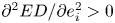 ${\partial ^{2}ED}/{\partial e_{i}^{2}}>0$, which represent the typical relationship between total emissions and environmental damage as suggested by many environmental economists.
As we consider environmental R&D, total emissions are given by  $ e_i=q_i-x_i-\beta x_j$, where
 $q_i$,
 $x_i$, and
 $\beta \in [0,1]$ are total polluting output, environmental R&D that mitigates pollution, and the spillover rate of technology, respectively, i=1,2,
 $i \neq j$. Therefore, when
 $\beta \neq 0$, firm i benefits from firm j's R&D effort by amount
 $\beta x_j$ for emission reductions, i=1,2,
 $i \neq j$.
We assume the cost of environmental R&D to be 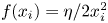 $f(x_{i})={\eta }/{2} x_{i}^{2}$, i=1,2, where
 $\eta >0$ represents efficiency of the environmental R&D technology. The inverse demand function is
 $p(q)=1-q$ where
 $q=q_{1}+q_{2}$ is total output of firms 1 and 2. The inverse demand function satisfies
 $p^{\prime \prime }(q)q+p^{\prime }(q)<0$, which guarantees the second-order condition for profit maximization. Additionally, in our setting of the model, the equilibrium is unique.
The payoff functions of firm i and country i are, respectively,  $\pi _{i}=pq_{i}-t_{i}e_{i}-f(x_{i})$ and
 $SW_{i}=\pi _{i}+t_{i}e_{i}-ED(e_{i})$, where
 $t_{i}e_{i}$ is the tax revenue, i=1,2. The property of a third-country model is that firms export all products to a third country, and consumer surplus can be ignored in the social welfare of country i,
 $ i=1,2$.
We examine four R&D scenarios studied by Kamien et al. (Reference Kamien, Muller and Zang1992):
• Scenario N: R&D competition. Firms compete during R&D given knowledge spillover
 $\beta \in \lbrack 0,1).$
• Scenario C: R&D cartel. Firms determine R&D investment cooperatively to maximize joint profit given knowledge spillover
$\beta \in \lbrack 0,1).$• Scenario NJ: RJV competition. Firms compete during R&D but share the outcome such that
$\beta =1.$• Scenario CJ: RJV cartel. Firms determine R&D investment cooperatively to maximize joint profit and share the R&D outcome, therefore,
$\beta =1.$


We study a three-stage game to document the four scenarios. We construct a three-stage game for scenario N and NJ (R&D/RJV competition). At stage 1, countries 1 and 2 simultaneously set tax rates  $t_{1}$ and
 $t_{2}$ to maximize their respective social welfares. At stage 2, firms decide their respective R&D investments (
 $x_{1}$ and
 $x_{2}$) independently to maximize individual profit. At stage 3, firms 1 and 2 determine their quantities of final goods (
 $q_{1}$ and
 $q_{2}$, respectively), and profits and social welfare result.
For scenario C and CJ (R&D/RJV cartel) the first and third stages repeat those of scenario N and NJ (R&D/RJV competition). However, at stage 2, firms form an environmental cartel and determine R&D to maximize joint profit  $\pi _{1}+\pi _{2}$.
For all scenarios we performed backward induction to find subgame perfect Nash equilibrium. We disregard cartel production because anti-monopoly laws prohibit it.Footnote 6
Although we analyze the models in the next section, equilibrium values for R&D/RJV competition and an R&D/RJV cartel appear in appendices A.1 and A.2, respectively.
4. R&D competition and RJV competition
At stage 3, the two firms choose  $q_{1}$ and
 $q_{2}$ as their respective profit-maximizing outputs. We get
 \begin{equation} \frac{\partial \pi _{i}}{\partial q_{i}}=p^{\prime }q_{i}+p-t_{i}=0,\quad i=1,2.\end{equation}
From equation (1), we obtain equilibrium output as  $q_{i}^{\ast }=\frac {1}{3} (1-2t_{i}+t_{j})$, i=1,2,
 $i\neq j$.
At stage 2, firms independently decide the environmental R&D spending that maximizes their respective profits. We obtain
 \begin{equation} \frac{\partial \pi _{i}}{\partial x_{i}}=t_{i}-\frac{\partial f}{\partial x_{i}}=0,\quad i=1,2.\end{equation}
Firm i decides what spending satisfies the condition that the marginal benefit of environmental R&D equals its marginal cost. From equation (2) and 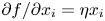 ${\partial f}/{\partial x_{i}}=\eta x_{i}$, we obtain equilibrium R&D as
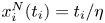 $x_{i}^{N}(t_{i})={t_{i}}/{\eta }$, i=1,2. Given that
 $t_{i}$ is the marginal benefit of R&D, we get
 ${\partial x_{i}^{N}}/{\partial t_{i}}={1}/{\eta }>0$. Benefits of environmental R&D come only from the reduced tax burden for end-of-pipe technologies.Footnote 7
At stage 1, countries establish  $t_{1}$ and
 $t_{2}$ as tax rates that maximize their respective social welfare:
 $$SW_{i}^{N}=p(q^{\ast })q_{i}^{\ast }-f(x_{i}^{N})-ED(q_{i}^{\ast}-x_{i}^{N}-\beta x_{j}^{N}), \quad i,j=1,2,\enspace i\neq j.$$
Footnote 8 We obtain
 \begin{equation} \frac{\partial SW_{i}^{N}}{\partial t_{i}}=(t_{i}-ED^{\prime }) \left(\frac{\partial q_{i}^{\ast }}{\partial t_{i}}-\frac{\partial x_{i}^{N}}{\partial t_{i}}\right)+\underbrace{p^{\prime}\frac{\partial q_{j}^{\ast }}{\partial t_{i}} q_{i}^{\ast }}_{(-)}=0,\quad i=1,2\ \mathrm{and}\ i\neq j.\end{equation}
See appendix A.3 for the derivation of equation (3).
The optimal environmental tax is
 \[ t_i^{N}(\beta)=\frac{\eta (-\eta +\gamma (3+2 \eta ))}{\gamma (3+3 \beta+\eta ) (3+2 \eta )+\eta (9+5 \eta )},\quad i=1,2. \]
When  $\beta =1$, we obtain the environmental tax under RJV competition as
 $ t_i^{NJ}=t_i^{N}(1)$.
As the last term of equation (3) is negative, the equilibrium tax rate is sub-Pigouvian because countries have incentives to extract rent from the rival firm when they act strategically (rent-shift effect), as indicated in Ulph (Reference Ulph1996).Footnote 9
When β increases, the marginal environmental damage lessens through knowledge spillover. As a result, the optimal environmental tax decreases in β, and we get  ${\partial t_i^{N}}/{\partial \beta }<0$.
In the equilibrium, we get  $x_i^{N}(\beta )=x_i^{N}(t_i^{N}(\beta ))$ and
 $ x_i^{NJ}=x_i^{N}(t_i^{N}(1))$. From
 ${\partial x_i^{N}}/{\partial t_i}>0$ and
 ${\partial t_i^{N}}/{\partial \beta }<0$, we obtain
 ${\partial x_i^{N}(\beta )}/{\partial \beta }={\partial x_i^{N}}/{\partial t_i} ({ \partial t_i^{N}}/{\partial \beta })<0$. Therefore, we obtain the following result.
Lemma 1: Environmental R&D is lower under RJV competition than under R&D competition. Therefore, we obtain 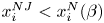 $x_i^{NJ}<x_i^{N}(\beta )$for
 $\beta \in [0,1)$, i=1.2.
5. R&D cartel and RJV cartel
The equilibrium output at stage 3 is the same as in the previous sections, and we obtain  $q_{i}^{\ast }=\frac {1}{3}(1-2t_{i}+t_{j})$, i=1,2 and
 $ i\neq j$. At stage 2, however, firms 1 and 2 choose
 $x_{1}$ and
 $x_{2}$, respectively, as their R&D spending to maximize joint profit
 $\pi _{1}+\pi _{2}$. We get
 \begin{equation} \frac{\partial \lbrack \pi _{i}+\pi _{j}]}{\partial x_{i}}=t_{i}+\beta t_{j}- \frac{\partial f}{\partial x_{i}}=0,\quad i,j=1,2\ \mathrm{and}\ i\neq j.\end{equation}
From equation (4), we obtain equilibrium environmental R&D as  $ x_{i}^{C}(t_{i},t_{j},\beta )={(t_{i}+\beta t_{j})}/{\eta }$.
Under an R&D/RJV cartel, firm i can receive the marginal benefit  $ t_{i}+\beta t_{j}$ from environmental R&D. Therefore, when firms form R&D/RJV cartels, they internalize knowledge spillover, which reduces a rival firm's tax burden. We thus obtain
 ${\partial x_{i}^{C}(t_{i},t_{j},\beta )}/{\partial t_{i}}={1}/{\eta }>0$,
 ${\partial x_{i}^{C}(t_{i},t_{j},\beta )}/{\partial t_{j}}={\beta }/{\eta } >0$ and
 ${\partial x_{i}^{C}(t_{i},t_{j},\beta )}/{\partial \beta }= {t_{j}}/{\beta }>0$; if the marginal benefit of environmental R&D increases,
 $x_{i}^{C}$ increases.
At stage 1, countries 1 and 2 simultaneously establish  $t_{1}$ and
 $t_{2}$, respectively, as welfare-maximizing environmental taxes. The social welfare of country i is
 $SW_{i}^{C}=p(q^{\ast })q_{i}^{\ast }-f(x_{i}^{C})-ED(q_{i}^{\ast }-x_{i}^{C}-\beta x_{j}^{C})$, and we get
 \begin{equation} \frac{\partial SW_{i}^{C}}{\partial t_{i}}=(t_{i}-ED^{\prime }) \left(\frac{\partial q_{i}^{\ast }}{\partial t_{i}}-\frac{\partial x_{i}^{C}}{\partial t_{i}}\right)+p^{\prime }\frac{\partial q_{j}^{\ast }}{\partial t_{i}}q_{i} \underbrace{-\beta t_{j}\frac{\partial x_{i}^{C}}{\partial t_{i}}}_{(-)}+ \underbrace{\beta ED^{\prime }\frac{\partial x_{j}^{C}}{\partial t_{i}}}_{(+)}=0,\end{equation}
i=1,2 and  $i\neq j$. See appendix A.3 for the derivation of equation (5).
The third and fourth terms in (5) differ from the examination of R&D/RJV competition (eqation (3)). The third term is the over-investment effect, which takes the tax rate beneath the Pigouvian level. Firms in R&D cartels consider benefits to rivals and increase R&D spending. From a social welfare perspective, however, that is over-investment. Therefore, governments set a lower tax rate to reduce R&D spending.Footnote 10
The fourth term is the environmental spillover effect (Ulph and Ulph, Reference Ulph and Ulph2007). The domestic environmental tax increases the rival firm's R&D through knowledge spillover, which in turn reduces domestic pollution. Therefore, governments have an incentive to set a higher tax rate. Using equation (5), symmetrical.
 \begin{equation} t_{i}^{C}=ED^{\prime }\frac{\frac{\partial q_{i}^{\ast }}{\partial t_{i}}- \frac{\partial x_{i}^{C}}{\partial t_{i}}-\beta \frac{\partial x_{j}^{C}}{ \partial t_{i}}}{\frac{\partial q_{i}^{\ast }}{\partial t_{i}}-\frac{ \partial x_{i}^{C}}{\partial t_{i}}-\beta \frac{\partial x_{i}^{C}}{\partial t_{i}}}-\frac{p^{\prime }\frac{\partial q_{j}^{\ast }}{\partial t_{i}} q_{i}^{\ast }}{\frac{\partial q_{i}^{\ast }}{\partial t_{i}}-(1+\beta ) \frac{\partial x_{i}^{C}}{\partial t_{i}}},\quad i,j=1,2\ \mathrm{and}\ i\neq j.\end{equation}
In equation (6), the fact that  ${\partial x_{i}^{C}}/{\partial t_{i}}= {1}/{\eta }\geq {\partial x_{j}^{C}}/{\partial t_{i}}={\beta }/{ \eta }$ means that the first term is less than or equal to
 $ED^{\prime }$ because the numerator
 ${\partial q_{i}^{\ast }}/{\partial t_{i}}-{\partial x_{i}^{C}}/{\partial t_{i}}-\beta ({\partial x_{j}^{C}}/{\partial t_{i}})$ is less than or equal to the denominator
 ${\partial q_{i}^{\ast }}/{\partial t_{i}}-{\partial x_{i}^{C}}/{\partial t_{i}}-\beta ({\partial x_{i}^{C}}/{\partial t_{i}})$. In addition, the second term is positive. Therefore, we obtain
 $t_{i}^{C}<ED_{i}^{\prime }$, meaning that the effects of rent-shift and over-investment dominate the environmental spillover effect.Footnote 11 The sign of
 ${\partial t_{i}^{C}}/{\partial \beta }$ is ambiguous.
In the equilibrium, we get  $x_i^{C}(\beta )=x_i^{C}(t_i^{C}(\beta ),t_j^{C}( \beta ),\beta )$ and
 $x_i^{CJ}=x_i^{C}(t_i^{C}(1),t_j^{C}(1),1)$, i=1,2,
 $i \neq j$.
6. Comparison of four R&D formations
This section investigates performance of an international R&D/RJV cartel. It derives policy implications of cooperative environmental R&D.
6.1. Comparison of environmental taxes
First we examine optimal environmental taxation under RJV competition and an RJV cartel.
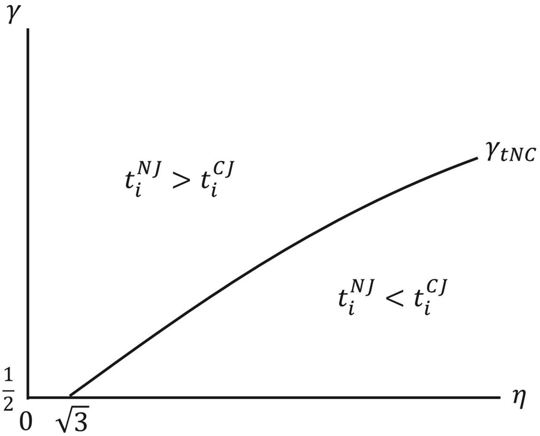
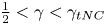
Proposition 1: When R&D efficiency is high (when  $\eta \leq \sqrt {3}$) or environmental damage is large (when
 $\gamma \geq \mathrm {max}\{\frac {1}{2},\gamma _{tNC}\}$), environmental tax under RJV competition exceeds taxation under an RJV cartel. When R&D efficiency is low (when
 $\eta >\sqrt {3}$) and environmental damage is small (when
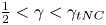 $\frac {1}{2}<\gamma <\gamma _{tNC}$), environmental tax under RJV competition is below that under an RJV cartel.
Proof. We obtain
 \begin{align*} t_i^{NJ}-t_i^{CJ} &=\frac{3 \eta (8 \gamma ^2 \eta ^2+36 \gamma ^2 \eta +36 \gamma ^2-4 \gamma \eta ^2-18 \gamma \eta -3 \eta ^2)}{(2 \gamma \eta ^2+15 \gamma \eta +18 \gamma +5 \eta ^2+9 \eta ) (2 \gamma \eta ^2+30 \gamma \eta +72 \gamma +5 \eta ^2+18 \eta )},\nonumber\\ &\quad i=1,2. \end{align*}
Therefore, for any given η, the sign of  $t_i^{NJ}-t_i^{CJ}$ is positive when γ is large. Then we obtain
 $\gamma _{tNC}={(2 \eta ^2+\sqrt {28 \eta ^4+144 \eta ^3+189 \eta ^2 }+9 \eta )}/{4 (2 \eta ^2+9 \eta +9)}$ which satisfies
 $t_i^{NJ}=t_i^{CJ}$, and
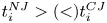 $t_i^{NJ}> (<) t_i^{CJ}$ when
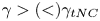 $\gamma > (<) \gamma _{tNC}$. In addition, we obtain
 $\eta =\sqrt {3}$ which satisfies
 $\gamma _{tNC}=\frac {1}{2}$ and
 ${\partial \gamma _{tNC}}/{\partial \eta }>0$ which leads to the result.□
Figure 1 depicts the result. The curve  $\gamma _{tNC}$ satisfies
 $ t_{i}^{NJ}=t_{i}^{CJ}$, i=1,2.
Proposition 1.

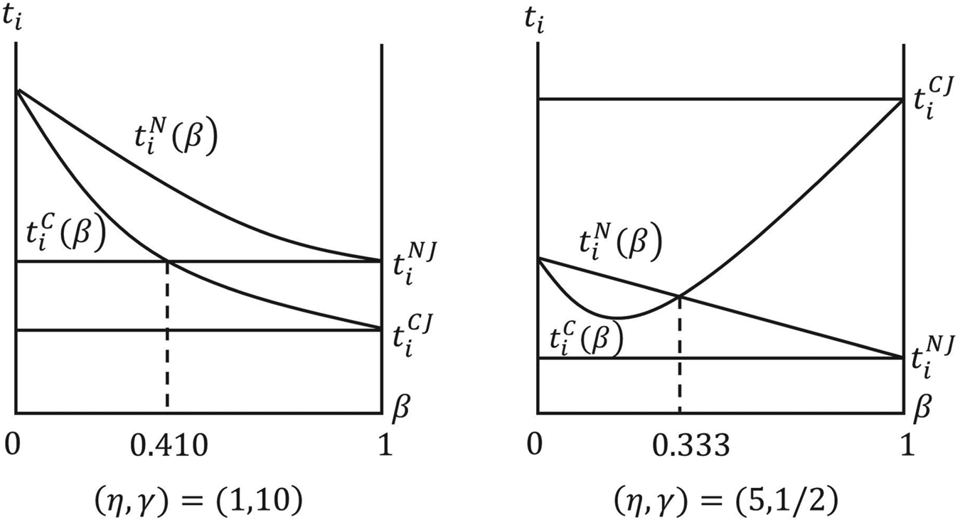
We explain our results as follows. Under R&D cartels, the sign of  ${\partial t_{i}^{C}}/{\partial \beta }$ depends on the parameters β, η, and γ.Footnote 12 When R&D efficiency is high (when
 $\eta \leq\sqrt {3}$) or environmental damage is large (when
 $\gamma \geq \mathrm {max}\{\frac {1}{2},\gamma _{tNC}\}$), environmental R&D is substantial and raises R&D spending. The over-investment effect is enhanced when β increases, and we obtain
 ${\partial t_{i}^{C}}/{\partial \beta }<0$ followed by
 $t_{i}^{NJ}>t_{i}^{CJ}$.
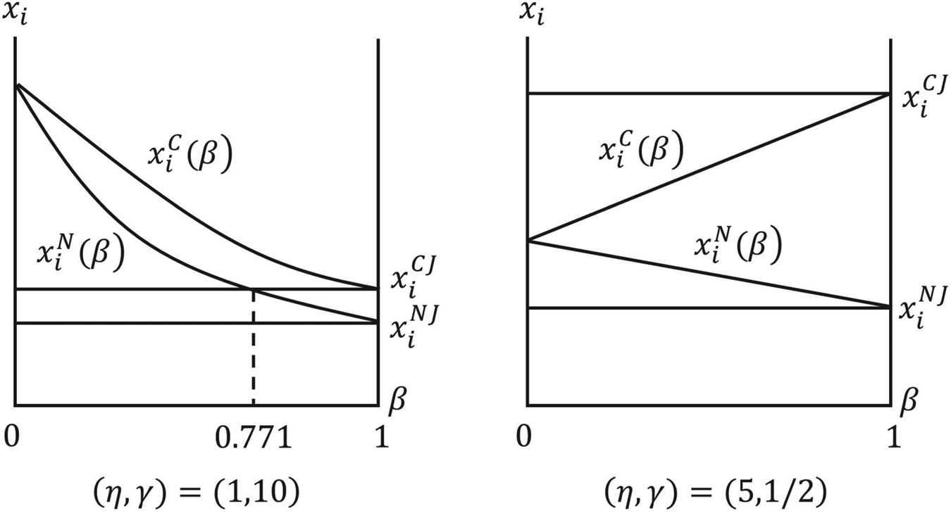
For example, when  $\eta =1$ and
 $\gamma =10$, we get
 ${\partial t_{i}^{C}}/{\partial \beta }<0$ as depicted in the left panel of figure 2. In this case, governments rely on knowledge spillover to lessen environmental damage and set the lower tax rate to suppress R&D spending under an R&D/RJV cartel. Therefore, we obtain
 $t_{i}^{NJ}>t_{i}^{CJ}$.
The relation between environmental tax and knowledge spillover.

When R&D efficiency is low (when  $\eta >\sqrt {3}$) and environmental damage is small (when
 $\frac {1}{2}<\gamma <\gamma _{tNC}$), environmental R&D is subdued. Environmental spillover effects are enhanced when β is large to promote environmental R&D of rival firms. Therefore, we obtain
 ${\partial t_i^{C}}/{\partial \beta }>0$ followed by
 $t_i^{NJ}<t_i^{CJ}$.
For example, when  $\eta =5$ and
 $\gamma =\frac {1}{2}$, then
 ${\partial t_{i}^{C}}/{\partial \beta }>0$ when β is large as depicted in the right panel of figure 2. In this case, governments set a higher environmental tax to promote rival firms' R&D investment under an R&D/RJV cartel. Therefore, we obtain
 $t_{i}^{NJ}<t_{i}^{CJ}$.
6.2. Comparison of R&D investment
We compare R&D spending under R&D/RJV competition with that under an R&D/RJV cartel. From our assumption of  ${\partial f}/{\partial x_{i}}>0$ and from equations (2) and (4), we obtain
 $x_{i}^{N}\leq x_{i}^{C}$ if and only if
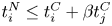 $t_{i}^{N}\leq t_{i}^{C}+\beta t_{j}^{C}$.Footnote 13 We obtain the following result.
Proposition 2: Environmental R&D is higher under an international R&D/RJV cartel than under R&D/RJV competition for any given β. Therefore, we obtain  $ x_{i}^{CJ}>x_{i}^{NJ}$and
 $x_{i}^{C}(\beta )\geq x_{i}^{N}(\beta )$for any given
 $\beta \in \lbrack 0,1)$, i=1,2.
The proof can be found in appendix A.4.
Previous literature shows that competition during R&D generates higher spending than cooperative R&D when knowledge spillover is small (D'Aspremont and Jacquemin, Reference D'Aspremont and Jacquemin1988; Chiou and Hu, Reference Chiou and Hu2001; Poyago-Theotoky, Reference Poyago-Theotoky2007; Ouchida and Goto, Reference Ouchida and Goto2016a). However, in our model which features strategic environmental policy, incentive for R&D spending under an R&D/RJV cartel always exceeds that under R&D/RJV competition, even if knowledge spillover is small. Alongside the benefit of internalization of knowledge spillover, the environmental spillover effect – which enhances environmental taxes under R&D/RJV cartels – prompts this result.Footnote 14
We also show that RJV cartels do not generate the highest R&D. We investigate how knowledge spillover affects R&D spending to show the result. In the case of R&D competition, we get  ${\partial x_i^{N}}/{\partial \beta }<0$ for any η and γ (see Lemma 1).
However, in the case of R&D cartels, the sign of  ${\partial x_i^{C}}/{\partial \beta }$ is ambiguous. To investigate the sign of
 ${\partial x_i^{C}}/{\partial \beta }$, we obtain this equation for i,j=1,2 and
 $i \neq j$:
 \begin{align} \frac{\partial x_{i}^{C}(t_{i}^{C}(\beta ),t_{j}^{C}(\beta ),\beta )}{\partial \beta } &= \underbrace{\frac{\partial x_{i}^{C}(t_{i},t_{j},\beta )}{\partial t_{i}} \frac{\partial t_{i}^{C}}{\partial \beta }}_{\mathrm{indirect~effect}}+ \underbrace{\frac{\partial x_{i}^{C}(t_{i},t_{j},\beta )}{\partial t_{j}} \frac{\partial t_{j}^{C}}{\partial \beta }}_{\mathrm{indirect~effect}}+ \underbrace{\frac{\partial x_{i}^{C}(t_{i},t_{j},\beta )}{\partial \beta }}_{\mathrm{direct~effect(+)}}.\end{align}
The first and second terms of equation (7) represent the effect of β on environmental R&D via tax rates. We obtain  ${\partial x_{i}^{C}(t_{i},t_{j},\beta )}/{\partial t_{i}}={1}/{\eta }>0$, whereas
 $ {\partial t_{i}^{C}}/{\partial \beta }$ depends on β, η and γ. Therefore, signs of indirect effects are ambiguous, but the direct effect (the third term) is positive. Therefore,
 ${\partial x_{i}^{C}(t_{i},t_{j},\beta )}/{\partial \beta }={t_{j}}/{\eta }>0$.
When R&D efficiency is high or environmental damage is large, over-spending leads to  ${\partial t_{i}^{C}}/{\partial \beta }<0$, which induces an indirect negative effect. In this case, we get
 ${\partial x_{i}^{C}}/{\partial \beta }<0$ if indirect effects dominate the direct effect.
For example, when  $\eta =1$ and
 $\gamma =10$, negative indirect effects dominate the positive direct effect, engendering
 ${\partial x_{i}^{C}}/{\partial \beta }<0$ as depicted in the left panel of figure 3. In this case, the rankings of environmental R&D are
 $x_{i}^{C}(\beta )\geq x_{i}^{N}(\beta )>x_{i}^{CJ}>x_{i}^{NJ}$ when
 $0\leq \beta <0.771$, and
 $ x_{i}^{C}(\beta )\geq x_{i}^{CJ}>x_{i}^{N}(\beta )>x_{i}^{NJ}$ when
 $ 0.771\leq \beta <1$. Therefore, RJV cartels do not generate the highest R&D.
The relation between R&D investment and knowledge spillover.

On the other hand, when R&D efficiency is low and environmental damage is small, the environmental spillover effect leads to  ${\partial t_{i}^{C} }/{\partial \beta }>0$ when β is large. In this case, indirect effects become positive, and we obtain
 ${\partial x_{i}^{C}}/{\partial \beta }>0$. For example, when
 $\eta =5$ and
 $\gamma =\frac {1}{2}$, we obtain
 ${\partial x_{i}^{C}}/{\partial \beta }>0$ as depicted in the right panel of figure 3. In this case, positive indirect effects and the direct effect generate the highest R&D under RJV cartels. Our result differs from that in D'Aspremont and Jacquemin (Reference D'Aspremont and Jacquemin1988), where an RJV cartel generates the highest R&D.
Ouchida and Goto (Reference Ouchida and Goto2016a) showed that environmental R&D under an RJV cartel is below that under R&D competition. In their model, however, governments cannot commit to a tax rate. Therefore, firms could affect tax rates. They chose higher environmental R&D to induce lower tax rates when competing during R&D. Firms cannot affect tax rates in our model.
6.3. Social welfare
Next, we compare social welfare under RJV competition and an RJV cartel.Footnote 15
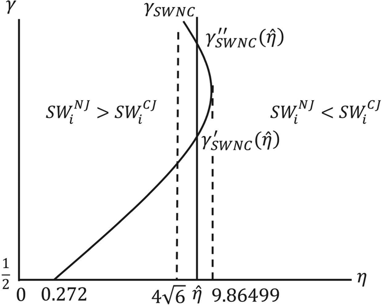
Proposition 3: When  $0<\eta \leq 4\sqrt {6}$, we obtain
 $SW_i^{NJ} \geq SW_i^{CJ}$if
 $ \gamma \geq \mathrm {max}\{\frac {1}{2},\gamma _{SWNC}\}$, i = 1, 2. When
 $4\sqrt {6 }<\eta \leq 9.86499$, we obtain
 $SW_i^{NJ} \geq SW_i^{CJ}$if
 $ \gamma _{SWNC}^{\prime }\leq \gamma \leq \gamma _{SWNC}^{\prime \prime }$,
 $i=1,2 $. Otherwise, we obtain
 $SW_i^{NJ} < SW_i^{CJ}$, i = 1, 2.
The proof is in appendix A.5.
Therefore, the highest environmental R&D under an RJV cartel does not always maximize social welfare. Figure 4 depicts the result for the  $(\eta ,\gamma )$ space. The curve
 $\gamma _{SWNC}$ satisfies
 $SW_{i}^{NJ}(\eta ,\gamma )=SW_{i}^{CJ}(\eta ,\gamma )$, i=1,2. Moreover, when
 $4\sqrt {6} <\eta <9.86499$, we obtain
 $\gamma _{SWNC}^{\prime }(\hat {\eta })$ and
 $ \gamma _{SWNC}^{\prime \prime }(\hat {\eta })$ such that
 $SW_{i}^{NJ}(\hat {\eta },\gamma )=SW_{i}^{CJ}(\hat {\eta },\gamma )$ for a given
 $\hat {\eta }\in (4 \sqrt {6},9.86499)$ where
 $\gamma _{SWNC}^{\prime }<\gamma _{SWNC}^{\prime \prime }$.
Proposition 3.

The following is the intuition of the result. Comparing social welfares, we obtain
 \begin{align} SW_{i}^{CJ}-SW_{i}^{NJ} =\underbrace{[p^{CJ}q_{i}^{CJ}-p^{NJ}q_{i}^{NJ}]}_{\Delta TR(?)} \underbrace{-[f(x_{i}^{CJ})-f(x_{i}^{NJ})]}_{\Delta f(-)} \underbrace{-[ED_{i}^{CJ}-ED_{i}^{NJ}]}_{\Delta ED(+)}.\end{align}
Given that  $x_{i}^{C}(\beta )\geq x_{i}^{N}(\beta )$ and
 ${\partial f}/{\partial x_{i}}>0$, the second term (difference in R&D cost) in equation (8) is negative. An RJV cartel entails a cost. Also, the last term in equation (8) is positive for any parameter in our specification. Therefore, less environmental damage is one benefit of an RJV cartel. Only the first term (difference in total revenue) in equation (8) is ambiguous.
When  $0<\eta \leq 4\sqrt {6}$ and
 $\gamma \geq \mathrm {max}\{\frac {1}{2},\gamma _{SWNC}\}$, or when
 $4\sqrt {6}<\eta \leq 9.86499$ and
 $\gamma _{SWNC}^{\prime }\leq \gamma \leq \gamma _{SWNC}^{\prime \prime }$, the over-investment effect and lesser environmental damage under an RJV cartel lead to
 $t_{i}^{NJ}>t_{i}^{CJ}$, which can result in
 $\Delta TR<0$. Therefore, environmental tax under an RJV cartel is excessively low with respect to rent extraction. As a result, we obtain
 $SW_{i}^{NJ}>SW_{i}^{CJ}$ even if
 $x_{i}^{NJ}<x_{i}^{CJ}$.
In general, RJV cartels maximize social welfare (D'Aspremont and Jacquemin, Reference D'Aspremont and Jacquemin1988; Kamien et al., Reference Kamien, Muller and Zang1992; Chiou and Hu, Reference Chiou and Hu2001; Poyago-Theotoky, Reference Poyago-Theotoky2007; Ouchida and Goto, Reference Ouchida and Goto2016a,Reference Ouchida and Gotob), because it internalizes two market failures caused by the public goods nature of knowledge. However, in international contexts where firms in different countries cooperate on environmental R&D and governments act strategically, RJV cartels may not engender the highest social welfare.
6.4. Global welfare
Although we show the case of  $SW_{i}^{NJ}\geq SW_{i}^{CJ}$, RJV cartels may be preferable to RJV competition from a global welfare perspective that includes consumer surplus in the third country.Footnote 16 We only show that social and global welfare conflict under the case of
 $\beta =1 $.
First, we define social welfare of the third country as  $SW_{3}^{k}=CS^{k}= \frac {1}{2}(q_{1}^{k}(t_{1}^{k},t_{2}^{k})+q_{2}^{k}(t_{1}^{k},t_{2}^{k}))^{2}$, where
 $ CS^{k}$ represents consumer surplus and k=N,NJ,C,CJ. From equation (2), we get
 $q_{1}^{k}+q_{2}^{k}=\frac {1}{3}(2-t_{1}^{k}-t_{2}^{k})$, k=N,NJ,C,CJ. Therefore, we obtain
 $SW_{3}^{NJ}\leq (>)SW_{3}^{CJ}$ if and only if
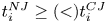 $ t_{i}^{NJ}\geq (<)t_{i}^{CJ}$.
Now, we consider global welfare (GW) as the summed social welfare of the three countries. Therefore,  $GW^{k}=SW_1^{k}+SW_2^{k}+SW_3^{k}$,
 $ k=N,NJ,C,CJ $.
Proposition 4: When  $\gamma \geq \mathrm {max}\{\frac {1}{2},\gamma _{GWNC}\}$, we obtain
 $ GW^{NJ} \leq GW^{CJ}$. Otherwise, we obtain
 $GW^{NJ}>GW^{CJ}$.
The proof can be found in appendix A.6.
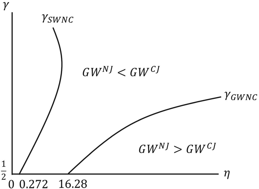
Figure 5 depicts results for the  $(\eta ,\gamma )$ space. The curve
 $\gamma _{GWNC}$ satisfies
 $GW^{NJ}(\eta ,\gamma )=GW^{CJ}(\eta ,\gamma )$. Figure 5 also depicts
 $\gamma _{SWNC}$ which appeared in figure 4. Therefore, when
 $ 0<\eta \leq 4\sqrt {6}$ and
 $\gamma \geq \mathrm {max}\{\frac {1}{2},\gamma _{SWNC}\}$, or when
 $4\sqrt {6}<\eta \leq 9.86499$ and
 $\gamma _{SWNC}^{\prime }\leq \gamma \leq \gamma _{SWNC}^{\prime \prime }$, we obtain
 $ SW_{i}^{NJ}\geq SW_{i}^{CJ}$ for i=1,2, whereas
 $GW^{NJ}<GW^{CJ}$. However, when
 $\frac {1}{2}<\gamma <\gamma _{GWNC}$, we obtain
 $ SW_{i}^{NJ}<SW_{i}^{CJ} $ for i=1,2, whereas
 $GW^{NJ}>GW^{CJ}$. Then, we derive policy implications for an international RJV cartel.
Proposition 5: When R&D efficiency is high and environmental damage is large (when  $0<\eta \leq 4\sqrt {6}$and
 $\gamma \geq \mathrm {max}\{\frac {1}{2},\gamma _{SWNC}\}$or when
 $4\sqrt {6}<\eta \leq 9.86499$and
 $\gamma _{SWNC}^{\prime }\leq \gamma \leq \gamma _{SWNC}^{\prime \prime }$), governments – including that of the third country – achieve higher global welfare by promoting RJV cartels. When R&D efficiency is low and environmental damage is small (when
 $\eta >16.28$and
 $\frac {1}{2}<\gamma <\gamma _{GWNC}$), governments enlarge global welfare by prohibiting RJV cartels.

This result is obtained from propositions 3 and 4.
Therefore, RJV cartels seem preferable to RJV competition for global welfare even if  $SW_i^{NJ}\geq SW_i^{CJ}$, but that is not always so. If an RJV cartel diminishes consumer surplus in the third country, promoting it contradicts the competition policy perspective.
Governments have recently promoted cooperative R&D to encourage international competitiveness, going so far as providing special antitrust treatment for it.Footnote 17 In addition, technology development and diffusion of environmental technology are indispensable for solving long-term environmental problems such as global warming. Therefore, banning RJV cartels may not serve the best interests of governments. If a strategic environmental policy exists, governments face tradeoffs between global welfare, especially consumer surplus in the third country, and promotion of environmental R&D. Therefore, our results suggest that governments, including that of the third country, should cooperate to determine whether to allow an R&D/RJV cartel.
6.5. Firms' incentives to form R&D/RJV cartels
Finally, we note firms' incentives to form R&D/RJV cartels. Comparing joint profit under R&D/RJV competition with that under an R&D/RJV cartel, we obtain  $\pi _1^{C}(t_1,t_2,\beta )+\pi _2^{C}(t_1,t_2,\beta ) -(\pi _1^{N}(t_1,t_2,\beta )+\pi _2^{N}(t_1,t_2,\beta ))={\beta ^2 (t_1^2+t_2 ^2)}/{2 \eta }>0$. Therefore, firms always choose R&D/RJV cartels for any given
 $\beta \in [0.1]$ when governments set environmental taxes before firms choose an R&D scenario.
However, if we consider a ‘no commitment’ case in which governments set environmental taxes after firms choose an R&D scenario, firms might not choose an R&D/RJV cartel. Absent governmental commitment, firms can affect environmental taxes. Therefore, firms may choose R&D/RJV competition expecting a higher environmental tax because it induces higher revenue than an R&D/RJV cartel.Footnote 18
On the other hand, in the model of Poyago-Theotoky (Reference Poyago-Theotoky2007), firms always have an incentive to form R&D/RJV cartels absent governmental commitment. Therefore, in international contexts where strategic environmental policy exists, governments should commit to the tax rate if they want to control cooperative R&D among firms.
7. Model extension
We now consider the case in which firms supply their products to markets in Country 1 and Country 2 plus the third country. We explain that our main result holds if the market of Country 3 exceeds that of Country 1 and Country 2. We assume the inverse demand function of Country i is  $ p_{i}=a-b(q_{i1}+q_{i2})$, i=1,2, and that of Country 3 is
 $ p_{3}=c-d(q_{31}+q_{32})$. The sign
 $q_{ij}$ represents the quantity of product firm j supplied to Country i, i=1,2,3 and j=1,2. The sign
 $ a,b$ and c,d represents market size of Countries 1, 2, and Country 3, respectively. We assume that the market sizes of Country 1 and 2 are identical. If a<c and b>d, the market size of Country i, i=1,2, is smaller than that of Country 3.
The social welfare of Country i is  $SW_{i}=({b}/{2})(q_{i1}+q_{i2})^{2}+ \pi _{i}+t_{i}(\sum _{k=1}^{3}q_{ki}-x_{i}-\beta x_{j})-ED(\sum _{k=1}^{3}q_{ki}-x_{i}-\beta x_{j})$, where
 $\pi _{i}=\sum _{k=1}^{3}p_{k}q_{ki}-t_{i}(\sum _{k=1}^{3}q_{ki}-x_{i}-\beta x_{j})-f(x_{i})$, i,j=1,2,
 $i\neq j$. Therefore, the social welfare of Country i includes consumer surplus. The social welfare of Country 3 is
 $ SW_{3}=({d}/{2})(q_{31}+q_{32})^{2}$.
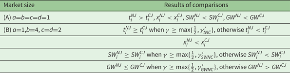
We investigate two cases: (A) the market sizes of the three countries are the same, and a=b=c=d=1; (B) the market size of Country 3 exceeds that of Countries 1 and 2, and a=1,b=4,c=d=2. The result appears in table 1. Equilibrium values for case (A) and case (B) appear in the online appendix.
Comparisons, where  $p_{i}=a-b(q_{i1}+q_{i2})$, i=1,2, and
 $ p_{3}=c-d(q_{31}+q_{32})$

In case (A), we obtain  $t_{i}^{NJ}>t_{i}^{CJ}$ and
 $SW_{i}^{NJ}<SW_{i}^{CJ}$ for any
 $\eta >0$ and
 $\gamma \geq \frac {1}{2}$, which differs from results for propositions 1 and 3. On the other hand, in case (B), we obtain qualitatively the same result as with propositions 1, 2, 3, 4, and 5.Footnote 19
Intuition for the result is as follows. When consumer surplus is included in social welfare, environmental taxes remedy distortions of imperfect competition.Footnote 20 If the market sizes of the three countries are identical, the government's incentive to remedy the distortion of imperfect competition cancels out the effect of strategic environmental policy (Greaker, Reference Greaker2013). In addition, environmental damage under an RJV cartel is below that under RJV competition. As a result, we obtain  $t_{i}^{NJ}>t_{i}^{CJ}$. Then we obtain
 $ SW_{i}^{NJ}<SW_{i}^{CJ}$ even if
 $t_{i}^{NJ}>t_{i}^{CJ}$, because the benefit of rent extraction is less than the loss of consumer surplus in its own country.
However, if the market of Country 3 is large, the effects of strategic environmental policy appear and we obtain the same result as with propositions 1, 2, 3, 4, and 5.
8. Conclusions
This paper examined relations between strategic environmental policy, international R&D cartels, and RJV using a third-country model featuring Cournot duopoly. We found that governments have three incentives that distort environmental policy when firms form an international R&D/RJV cartel. We derive three implications for international environmental technology policy.
First, and contrary to conventional wisdom, RJV cartels do not necessarily maximize social welfare. We show that strategic environmental policy (over-investment effect) reduces social welfare under an RJV cartel compared to RJV competition, whereas environmental investment under an R&D/RVJ cartel is higher than under R&D/RJV competition. Therefore, there are tradeoffs between social welfare and environmental R&D.
Second, governments, including that of the third country, can enhance global welfare if they collectively decide whether to allow R&D/RJV cartels. Collective decision-making enhances consumer surplus in the third country.
Finally, in international contexts where strategic environmental policy exists, governments should commit to an environmental tax rate to promote forming R&D/RJV cartels.
Supplementary material
The supplementary material for this article can be found at https://doi.org/10.1017/S1355770X20000145
Acknowledgments
The author would like to thank two anonymous referees; Akira Miyaoka, Kenji Takeuchi and Takayoshi Shinkuma; and the participants at the SEEPS2016 (Japan), Rokko Environmental Economics and Policy Seminar (Japan), and EAERE2017 (Greece), for helpful comments and suggestions. This research is supported by JSPS KAKENHI Grant Number 15K17046, and the Dean's Discretionary Fund of the School of Global and Community Studies at the University of Fukui. The usual disclaimer applies.
Appendix
A.1 R&D/RJV competition
In equilibrium, we obtain the equilibrium values as follows:
 \begin{equation} \begin{aligned} q_{i}^{N} & = \frac{(\gamma +\beta \gamma +\eta )(3+2\eta )}{\gamma (3+3\beta+\eta )(3+2\eta )+\eta (9+5\eta )},\\ x_{i}^{N} & = \frac{(-\eta +\gamma (3+2\eta))}{\gamma(3+3\beta +\eta )(3+2\eta )+\eta (9+5\eta )},\\ \pi _{i}^{N} & = \frac{A+\gamma^2(2\eta+3)^2(2\beta^2+2\beta(\eta+2)+\eta+2)+\eta^2((2\beta+25)\eta+8\eta^2+18)}{2(\gamma(2\eta+3)(3\beta+\eta+3)+\eta(5\eta+9))^2}, \end{aligned}\end{equation}
and
 \[ SW_{i}^{N}=\frac{\left( \eta ^{2}\left( 18+17\eta +4\eta ^{2}\right) + \gamma^{2}(3+2\eta )^{2}\left( 2+2\beta ^{2}+\eta +2\beta (2+\eta )\right) + \gamma B\right) }{2(\gamma (3+3\beta +\eta )(3+2\eta )+\eta (9+5\eta ))^{2}}, \]
where  $A \equiv 2 \gamma \eta (2 \eta +3) (2 \beta (\eta +3)+3 (\eta +2))$ and
 $B\equiv \eta (36+50\eta -\beta ^{2}\eta +24\eta ^{2}+4\eta ^{3}+\beta (36+34\eta +8\eta ^{2}))$, and i=1,2.
Note that global welfare is obtained as  $GW^{N}=\frac {1}{2} (q_1^{N}+q_2^{N})^2+SW_1^{N}+SW_2^{N}$.
A.2 R&D/RJV cartel
The optimal environmental tax under an R&D/RJV cartel is obtained as follows:
 \[ t_{i}^{C}=\frac{\eta \left( -\eta +\gamma \left( 3+3\beta ^{2}+2\eta \right)\right) }{\begin{matrix}\eta (9+9\beta +5\eta )\\+\gamma \left( 9+18\beta ^{3}+9\beta^{4}+9\eta +2\eta ^{2}+ 9\beta ^{2}(2+\eta )+6\beta (3+2\eta )\right) \end{matrix}},\quad i=1,2. \]
Then, we obtain the equilibrium values for i=1,2 as follows:
 \begin{align} q_{i}^{C} & = \frac{1}{3}\left(1-\frac{\eta \left(1-\eta +\gamma \left( 3+3\beta^{2}+2\eta \right) \right) }{\begin{matrix}\eta (9+9\beta +5\eta )\\+\gamma \left( 9+18\beta^{3}+9\beta ^{4}+9\eta +2\eta ^{2}+9\beta ^{2}(2+\eta )+6\beta (3+2\eta)\right) \end{matrix}}\right),\nonumber\\ x_{i}^{C} & = \frac{(1+\beta)\left( -\eta +\gamma \left(3+3\beta^{2}+2\eta\right)\right)}{\eta (9+9\beta +5\eta )+\gamma \left(9+18\beta^{3}+9\beta ^{4}+9\eta+2\eta ^{2}+9\beta^{2} (2+\eta)+6\beta (3+2\eta)\right)},\\ \pi _{i}^{C} & = \frac{\left( D+6(1+\beta)^{2}\gamma G+\eta ^{2} \left(18+25\eta +8\eta ^{2}+\beta ^{2}(18+\eta )+\beta (36+26\eta )\right)\right)}{\begin{matrix}2\left(\eta (9+9\beta +5\eta )\right.\\\left.+\gamma \left( 9+18\beta ^{3}+9\beta^{4}+9\eta +2\eta ^{2}+9\beta ^{2} (2+\eta)+6\beta (3+2\eta )\right)\right)^{2}\end{matrix}},\nonumber \end{align}
where  $D\equiv (1+\beta )^{2}\gamma ^{2}(2+4\beta +2\beta ^{2}+\eta )(3+3\beta ^{2}+2\eta )^{2}$,
 \[ SW_{i}^{C}=\frac{\left( D+\eta ^{2}\left( 18-\beta ^{2}(-18+\eta )+17\eta +4\eta ^{2}+4\beta (9+4\eta )\right) +\gamma H\right) }{\begin{matrix}2\left( \eta (9+9\beta +5\eta )\right.\\+\left.\gamma \left( 9+18\beta ^{3}+9\beta ^{4}+9\eta +2\eta^{2}+9\beta ^{2}(2+\eta )+6\beta (3+2\eta )\right) \right) ^{2}\end{matrix}}, \]
where  $G\equiv \eta (6+6\beta ^{3}+7\eta +2\eta ^{2} + 3\beta ^{2}(2 + \eta )+ \beta (6 + 4 \eta))$, and
 $H\equiv \eta (36+36\beta ^{5}+50\eta +24\eta ^{2}+4\eta ^{3}+16\beta ^{3}(9+5\eta )+\beta ^{4}(108+23\eta )+3\beta ^{2}(48+35\eta +8\eta ^{2})+2\beta (54+\break 49\eta +12\eta ^{2}))$.
Note that global welfare is obtained as  $GW^{C}=\frac {1}{2} (q_1^{C}+q_2^{C})^2+SW_1^{C}+SW_2^{C}$.
A.3 Derivation of equations (3) and (5)
Country i chooses  $t_{i}$ to maximize the social welfare
 $SW_{i}^{N}$, and we get
 \[ \frac{\partial SW_{i}^{N}}{\partial t_{i}}=(p^{\prime }q_{i}^{\ast }+p^{\ast}) \frac{\partial q_{i}^{\ast }}{\partial t_{i}}+p^{\prime }\frac{\partial q_{j}^{\ast }}{\partial t_{i}}q_{i}^{\ast }-\frac{\partial f}{\partial x_{i}} \frac{\partial x_{i}^{N}}{\partial t_{i}}-ED^{\prime }\left(\frac{\partial q_{i}^{\ast }}{\partial t_{i}}-\frac{\partial x_{i}^{N}}{\partial t_{i}}\right)=0, \]
i,j=1,2 and  $i\neq j$. From equations (1) and (2), we get
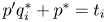 $p^{\prime }q_{i}^{\ast }+p^{\ast }=t_{i}$ and
 ${\partial f}/{\partial x_{i}}=t_{i}$, respectively. As a result, we get equation (3).
Country i chooses  $t_{i}$ to maximize the social welfare
 $SW_{i}^{C}$, and we get
 \[ \frac{\partial SW_{i}^{C}}{\partial t_{i}}=(p^{\prime }q_{i}^{\ast }+p^{\ast}) \frac{\partial q_{i}^{\ast }}{\partial t_{i}}+p^{\prime} \frac{\partial q_{j}^{\ast }}{\partial t_{i}}q_{i}^{\ast}- \frac{\partial f}{\partial x_{i}}\frac{\partial x_{i}^{C}}{\partial t_{i}}-ED^{\prime} \left(\frac{\partial q_{i}^{\ast }}{\partial t_{i}}-\frac{\partial x_{i}^{C}}{\partial t_{i}} -\beta \frac{\partial x_{j}^{C}}{\partial t_{i}}\right)=0, \]
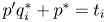
i,j=1,2 and  $i\neq j$. From equations (1) and (4), we obtain
 $p^{\prime }q_{i}^{\ast }+p^{\ast }=t_{i}$ and
 ${\partial f}/{\partial x_{i}} =t_{i}+\beta t_{j}$, respectively. As a result, we get equation (5).
A.4 Proof of proposition 2
Using equations (A1) and (A2), we obtain
 \[ x_{i}^{C}-x_{i}^{N}=\frac{\beta \eta (J-\eta ^{2}(5-8\gamma -4\gamma ^{2}))}{(6\beta \gamma \eta +9\beta \gamma +2\gamma \eta ^{2}+9\gamma \eta +9\gamma+5\eta ^{2}+9\eta )K}, \]
where  $J\equiv 9\beta ^{3}\gamma +6\beta ^{2}\gamma ^{2}\eta +9\beta ^{2}\gamma ^{2}+15\beta ^{2}\gamma \eta +45\beta ^{2}\gamma +18\beta \gamma \eta +36\beta \gamma +12\gamma ^{2}\eta +\break 9\gamma ^{2}+12\gamma \eta $ and
 $ K\equiv 9\beta ^{4}\gamma +18\beta ^{3}\gamma +9\beta ^{2}\gamma \eta +18\beta ^{2}\gamma +12\beta \gamma \eta +18\beta \gamma +9\beta \eta +\break 2\gamma \eta ^{2}+9\gamma \eta +9\gamma +5\eta ^{2}+9\eta $. Also, we obtain J>0, K>0 and
 $-\eta ^{2}(5-8\gamma -4\gamma ^{2})\geq 0$ when
 $ \gamma \geq \frac {1}{2}$. Therefore, we obtain
 $x_{i}^{C}(\beta )\geq x_{i}^{N}(\beta )$ for
 $\beta \in \lbrack 0,1]$.
A.5 Proof of proposition 3
Comparing  $SW_{i}^{NJ}$ with
 $SW_{i}^{CJ}$, we obtain
 \begin{align} & SW_{i}^{NJ}-SW_{i}^{CJ} \nonumber\\ &\quad =\frac{-\eta (L+M+O+Q)}{2\left( 2\gamma \eta^{2}+15\gamma \eta +18\gamma +5\eta ^{2}+9\eta \right) ^{2}\left( 2\gamma \eta ^{2}+30\gamma \eta +72\gamma +5\eta ^{2}+18\eta \right)^{2}},\end{align}
where  $L=\gamma ( 196\eta ^{3}+1881\eta ^{2}+6588\eta +7128) \eta ^{3}+3( 5\eta ^{2}+66\eta +108) \eta ^{4}>0$,
 $M=\break 4\gamma ^{4}( \eta ^{2}-96) ( 2\eta ^{2}+9\eta +9) ^{2}$,
 $O=3\gamma ^{2}\eta ^{2}( -8\eta ^{4}+420\eta ^{3}+4183\eta ^{2}+12996\eta +12636) $ and
 $Q=12\gamma ^{3}\eta ( -30\eta ^{4}-49\eta ^{3}+1017\eta ^{2}+4122\eta +4212)$.
Because the denominator of equation (A3) is positive, we obtain sign $ [SW_{i}^{NJ}-SW_{i}^{CJ}] = {\rm sign}[-\eta (L+M+O+Q)]$. Therefore, we investigate the sign of L+M+O+Q.
When  $\gamma =\frac {1}{2}$, we obtain
 $L+M+O+Q \leq (>)0$ if
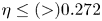 $\eta \leq (>) 0.272$. Therefore, when
 $\gamma =\frac {1}{2}$, we obtain
 $SW_i^{NJ} \geq (<)SW_i^{CJ}$ if
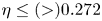 $\eta \leq (>)0.272$, i=1,2.
On the other hand, when  $\gamma \rightarrow \infty $, we obtain
 $L+M+O+Q=( \eta ^{2}-96) ( 2\eta ^{2} \break +9\eta +9) ^{2}\infty $. Therefore, when
 $\gamma \rightarrow \infty $, we obtain
 $ L+M+O+Q\leq (>)0$ if
 $\eta \leq\break (>)4\sqrt {6}$. This result comes from the effect of M because the degree of M about γ is the largest compared to L, O and Q. Therefore, when γ is sufficiently large, the sign of M dominates the signs of L, O and Q. When
 $\eta <(>)4\sqrt {6}$, we obtain
 $M<(>)0$ and
 ${\partial M}/{\partial \gamma } <(>)0$. As a result, when γ is sufficiently large, we obtain
 $ L+M+O+Q<0$ for any given
 $\eta <4\sqrt {6}$, and L+M+O+Q>0 for any given
 $ \eta >4\sqrt {6}$.
Note that the effect of sign M depends on the size of η. When η approaches  $4\sqrt {6}$, M becomes 0. Therefore, when η is sufficiently smaller than
 $4\sqrt {6}$ or η is sufficiently larger than
 $4\sqrt {6}$, the effect of M is large. When
 $\eta =0$, we obtain
 $ M+L+O+Q<0(M=-31104\gamma ^{4}$ and
 $L=O=Q=0)$ for any
 $\gamma \geq \frac {1}{2}$. Therefore, when η is small, especially when
 $\eta \leq 0.272$, we obtain
 $M+L+O+Q\leq 0$ for any
 $\gamma \geq \frac {1}{2}$.
Next, we consider the range of  $0.272<\eta \leq 4\sqrt {6}$. When η approaches
 $4\sqrt {6}$, M becomes 0. In this case, the signs of L, O and Q are important. When
 $\eta =4\sqrt {6}$, we obtain M=0,
 $L=384\sqrt {6 }( 101616\sqrt {6}+187704) \gamma +27648( 264\sqrt {6} +588) >0$,
 $O=288( 213264\sqrt {6}+340476) \gamma ^{2}>0$ and
 $Q=-48\sqrt {6}( 2328\sqrt {6}+174636) \gamma ^{3}<0$. Therefore, in this case, if
 $\gamma =0$, we obtain L>0, O=0 and Q=0. As a result, when
 $\eta =4\sqrt {6}$, we obtain L+M+O+Q>0 if γ is sufficiently small. However, when γ increases, because the degree of Q about γ is the largest compared to L and O, the sign of Q<0 dominates the signs of L>0 and O>0. Therefore, when
 $\eta =4\sqrt {6}$, we obtain L+M+O+Q<0 if γ is sufficiently large.
As a result, when  $0.272<\eta \leq 4\sqrt {6}$, we obtain
 $\gamma _{SWNC}(\eta )$ such that L+M+O+Q=0, and
 $L+M+O+Q<(>)0$ when
 $\gamma >(<)\gamma _{SWNC}(\eta )$. In addition, when η approaches
 $4\sqrt {6}$, because the effect of M that induces L+M+O+Q<0 becomes small, the large γ is required to obtain L+M+O+Q<0. Therefore, we obtain
 ${\partial \gamma _{SWNC}}/{\partial \eta }>0$ when
 $0.272<\eta \leq 4 \sqrt {6}$, as depicted in figure 4.
Next we consider the range of  $\eta >4\sqrt {6}$. When
 $\eta =4\sqrt {6} +\varepsilon $, where
 $\varepsilon >0$ is sufficiently small, we obtain L>0, M>0, O>0 and Q<0. In this case, as argued above, we obtain
 $ L+M+O+Q>0 $ when γ is sufficiently small, and L+M+O+Q>0 when γ is sufficiently large. However, when γ is in a certain range, we obtain L+M+O+Q<0. This is because the effect of Q<0 dominates the signs of L>0, M>0 and O>0. For example, when
 $\eta =9.8$, we obtain L+M+O+Q<0 when
 $13.291<\gamma <1573.97$. However, when
 $\eta \geq 9.86499$, we obtain
 $L+M+O+Q\geq 0$ for any γ.
As a result, for a given  $\hat {\eta }\in (4\sqrt {6},9.86499)$, we obtain
 $ \gamma _{SWNC}^{\prime }(\hat {\eta })$ and
 $\gamma _{SWNC}^{\prime \prime }( \hat {\eta })$ such that L+M+O+Q=0, where
 $\gamma _{SWNC}^{\prime }(\hat {\eta })<\gamma _{SWNC}^{\prime \prime }(\hat {\eta })$, and L+M+O+Q<0 when
 $ \gamma _{SWNC}^{\prime }(\hat {\eta })<\gamma <\gamma _{SWNC}^{\prime \prime }( \hat {\eta })$. Otherwise, we obtain L+M+O+Q>0. Therefore, when
 $4\sqrt {6} <\eta <9.86499$,
 $\gamma _{SWNC}(\eta )$ becomes a backward-bending curve as depicted in figure 4.
Finally, when  $\eta \geq 9.86499$, we obtain
 $L+M+O+Q \geq 0$ for any γ because the effect of M>0 is large. Indeed, when
 $\eta \rightarrow \infty $, we obtain
 $(16 \gamma ^4-24 \gamma ^2+196 \gamma +15) \infty >0 $ for any
 $\gamma \geq 0$.
A.6 Proof of proposition 4
Comparing  $GW^{NJ}$ with
 $GW^{CJ}$, we obtain
 \begin{align} & GW^{NJ}-GW^{CJ} \nonumber \\ &\quad =\frac{-\eta (R+S+T+U+W)}{\left( 2\gamma \left( \eta^{2}+15\eta +36\right) +\eta (5\eta +18)\right) ^{2}\left( \gamma \left(2\eta ^{2}+15\eta +18\right) +\eta (5\eta +9)\right) ^{2}},\end{align}
where  $R=4\gamma ^{4}(\eta ^{2}+24\eta +96)(2\eta ^{2}+9\eta +9)^{2}>0$,
 $ S=-3\eta ^{4}(35\eta ^{2}+132\eta +108)<0$,
 $T=-3\gamma \eta ^{3}(4\eta ^{3}+213\eta ^{2}+588\eta +216)<0$,
 $U=\gamma ^{2}\eta ^{2}(232\eta ^{4}+2508\eta ^{3}+9765\eta ^{2}+19332\eta +17172)>0$, and
 $W=4\gamma ^{3}\eta (32\eta ^{5}+678\eta ^{4}+4821\eta ^{3}+15795\eta ^{2}+25326\eta +16524)>0$.
Because the denominator of equation (A4) is positive, we obtain  ${\rm sign}[GW^{NJ}-GW^{CJ}]={\rm sign}[-\eta (R+S+T+U+W)]$. Therefore, we investigate the sign of R+S+T+U+W.
When  $\gamma \rightarrow \infty $, we obtain
 $R+S+T+U+W=(\eta ^2+24 \eta +96) (2 \eta ^2+9 \eta +\break 9)^2 \infty >0$. This is because the degrees of R>0, U>0 and W>0 about γ are larger than those of
 $ S<0$ and T<0. Therefore, when γ is sufficiently large, we obtain
 $ R+S+T+U+W>0$ for any η.
However, when γ is sufficiently small, the sign of R+S+T+U+W depends on the size of η. When  $\gamma = \frac {1}{2}$, we obtain
 $ R+S+T+U+W <0 (\geq )0$ if
 $\eta >(\leq )16.283$. This is because the effects of S<0 and T<0 become large when η increases. Therefore, when
 $\eta >16.283$, the large γ is required to obtain R+S+T+U+W>0. Then, we obtain
 $R+S+T+U+W=(16 \gamma ^4+128 \gamma ^3+232 \gamma ^2-12 \gamma -105) \infty $ when
 $\eta \rightarrow \infty $. Therefore, when
 $\eta \rightarrow \infty $, we obtain
 $R+S+T+U+W \geq (<)0$ when
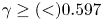 $\gamma \geq (<)0.597$. As a result, when
 $\gamma \geq 0.597$, we obtain
 $R+S+T+U+W \geq 0 $ for any η.
On the other hand, when η decreases, the effects of S<0 and T<0 become small. When  $\eta =0$, we obtain R+S+T+U+W>0 (
 $R=31104 \gamma ^4>0$ and S=T=U=W=0) for any γ. Therefore, when η is small, especially, when
 $\eta \leq 16.283$, the signs of R>0, U>0 and W>0 dominate those of S<0 and T<0, and we obtain
 $R+S+T+U+W \geq 0$ for any
 $\gamma \geq \frac {1}{2}$.
Finally, when  $\eta >16.283$ and
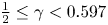 $\frac {1}{2}\leq \gamma <0.597$, we obtain
 $\gamma _{GWNC}(\eta )$ such that R+S+T+U+W=0, and
 $R+S+T+U+W\leq (>)0$ when
 $\gamma \leq (>)\gamma _{GWNC}$. In addition, when η increases, because the effects of S<0 and T<0 become large, the large γ is required to obtain R+S+T+U+W>0. Therefore, we obtain
 ${\partial \gamma _{GWNC}}/{\partial \eta }>0$ as depicted in figure 5.