1. Introduction
To study the interaction between electromagnetic fields and metallic (nano-)objects, it is possible, as a first approximation, to model the conduction electrons as a free electron plasma confined by the attractive Coulomb forces of the nuclei. However, the electrons carry, besides an electric charge, also a half-integer spin, which can play a significant role in their dynamics, most notably for intense and ultrashort laser pulses. Spin effects play an important role through the Zeeman effect, the spin-orbit interaction (Hinschberger & Hervieux Reference Hinschberger and Hervieux2012; Krieger et al. Reference Krieger, Dewhurst, Elliott, Sharma and Gross2015, Reference Krieger, Elliott, Müller, Singh, Dewhurst, Gross and Sharma2017) and spin currents (Choi et al. Reference Choi, Min, Lee and Cahill2014; Schellekens et al. Reference Schellekens, Kuiper, De Wit and Koopmans2014; Hurst, Hervieux & Manfredi Reference Hurst, Hervieux and Manfredi2018), and they are involved in the complex mechanisms leading to the loss of magnetization on a femtosecond time scale (Beaurepaire et al. Reference Beaurepaire, Merle, Daunois and Bigot1996; Bigot, Vomir & Beaurepaire Reference Bigot, Vomir and Beaurepaire2009; Bigot & Vomir Reference Bigot and Vomir2013).
Spin effects are usually described using standard approaches, such as the Hartree–Fock equations and the time-dependent density functional theory (Krieger et al. Reference Krieger, Dewhurst, Elliott, Sharma and Gross2015), or, more recently, quantum hydrodynamic models (Moldabekov, Bonitz & Ramazanov Reference Moldabekov, Bonitz and Ramazanov2018). In recent years, phase-space approaches issued from plasma physics research have been introduced as an alternative to the above models. These models make use of kinetic equations similar to the standard Vlasov equation, which describes the evolution of a probability distribution in the relevant phase space, and can be broadly grouped into two families: (i) models that use a scalar distribution function defined on an extended phase space $(\boldsymbol {x}, \boldsymbol {p}, \boldsymbol {s})$ , where $\boldsymbol {x}$
 denotes the position, $\boldsymbol {p}$
 the momentum and $\boldsymbol {s}$
 the spin variable on the unit sphere (Brodin et al. Reference Brodin, Marklund, Zamanian, Ericsson and Mana2008, Reference Brodin, Marklund, Zamanian and Stefan2011; Marklund, Zamanian & Brodin Reference Marklund, Zamanian and Brodin2010; Zamanian, Marklund & Brodin Reference Zamanian, Marklund and Brodin2010); (ii) models for which the distribution function is a $2\times 2$
 matrix that evolves in the standard classical phase space $(\boldsymbol {x}, \boldsymbol {p})$
 (Hurst et al. Reference Hurst, Morandi, Manfredi and Hervieux2014; Manfredi, Hervieux & Hurst Reference Manfredi, Hervieux and Hurst2019); this $2\times 2$
 distribution function can also be represented, in the so-called Pauli basis, as one scalar function $f_0$
 and one three-component vector function $\boldsymbol f$
 , for which reason we shall term these models ‘vectorial’. For both approaches, one assumes that the orbital motion is classical (hence the use of a standard Vlasov-like probability distribution), while the spin is treated as a fully quantum variable.
The relationship between the two types of models was not hitherto perfectly clear, in particular under what assumptions they are exactly equivalent. The first part of the present work will be devoted to clarify this important issue. Indeed, the vectorial distribution functions can be seen as the zeroth- and first-order ‘moments’ (in spin space) of the scalar distribution function $f(\boldsymbol {x}, \boldsymbol {p}, \boldsymbol {s})$ , and the vectorial equations as the evolution equations for such moments. This is the same relationship that exists between the Vlasov distribution function and its velocity moments, which obey a set of fluid equations. In the Vlasov/fluid analogy, the velocity moment equations are not equivalent to the full kinetic model, except if one prescribes a closure relation and this relation is preserved by the evolution of the kinetic equation.Footnote 1 In our spin case, the closure relation implies that the scalar distribution function $f(\boldsymbol {x}, \boldsymbol {p}, \boldsymbol {s})$
 should be a linear function of $\boldsymbol {s}$
 (Zamanian et al. Reference Zamanian, Marklund and Brodin2010; Manfredi et al. Reference Manfredi, Hervieux and Hurst2019). When this relation is satisfied for all times, taking the zeroth- and first-order moments of the scalar distribution leads to the evolution equations of the vectorial model and guarantees the equivalence between the two approaches. This important point will be discussed in detail in this work, in particular the role played by the quantum magnetic dipole term in the scalar model (which contains derivatives in both real and spin space, thus making particle-in-cell (PIC) methods much more involved).
From a numerical point of view, the two approaches are intrinsically different, and have their own advantages and drawbacks with respect to the available numerical techniques. Indeed, due to the high dimensionality of the extended phase space (three dimensions for position, three for momentum, and two for the spin), the scalar model is not adapted to grid-based (Eulerian) numerical methods. Instead, they are naturally adapted for PIC methods (Crouseilles et al. Reference Crouseilles, Hervieux, Li, Manfredi and Sun2021), for which the extra number of dimensions is not an obstacle as it only represents two more (spin) labels for the trajectories. In contrast, the vectorial approach is more easily amenable to Eulerian solvers, since it merely implies the solution of four Vlasov equations instead of one for spinless particles. Moreover, the presence of the quantum magnetic dipole term (involving cross-derivatives in both $\boldsymbol {p}$ and $\boldsymbol {s}$
 ) makes the scalar model quite awkward to solve numerically, whereas the corresponding term in the vector model does not raise any particular difficulty. For this reason, in our earlier work using a PIC code (Crouseilles et al. Reference Crouseilles, Hervieux, Li, Manfredi and Sun2021) this additional term was not taken into account.
We note that other PIC approaches (Brodin, Holkundkar & Marklund Reference Brodin, Holkundkar and Marklund2013) did not employ the extended phase space mentioned above, but considered two separate spin-up and spin-down populations for the electrons. Similarly, Tonge, Dauger & Decyk (Reference Tonge, Dauger and Decyk2004) and Dauger, Decyk & Dawson (Reference Dauger, Decyk and Dawson2005) have extended classical PIC methods to the quantum regime (without spin) using an approach based on Feynman path integrals. Very recently, PIC simulation methods for particles with spin were developed and validated by (Li et al. Reference Li, Decyk, Miller, Tableman, Tsung, Vranic, Fonseca and Mori2021) for applications to laser–plasma interactions.
In the present work, we propose an Eulerian method to solve numerically the self-consistent vectorial spin-Vlasov–Maxwell equations in the broad context of laser–plasma interactions. As the full six-dimensional phase space is still very demanding for Eulerian methods in terms of computational costs, we have considered a simpler one-dimensional (1-D) problem (two-dimensional phase space) obtained by assuming that the electrons are cold in the transverse plane with respect to the direction of propagation of the incident electromagnetic field. This model is thus described by the distribution functions $(f_0, {\boldsymbol {f}})(t, { x}, { p})\in \mathbb {R}^4$ , with $t\geq 0$
 and $({ x}, { p}) \in \mathbb {R}^2$
 .
The vectorial model enjoys a Poisson structure which paves the way to a suitable time splitting integrator. Following the recent development of geometric numerical method for Vlasov-type equations (Crouseilles, Einkemmer & Faou Reference Crouseilles, Einkemmer and Faou2015; Li, Sun & Crouseilles Reference Li, Sun and Crouseilles2020; Crestetto et al. Reference Crestetto, Crouseilles, Li and Massot2022), we first discretize in time by using a Hamiltonian splitting, which leads to different subsystems to solve. It turns out that the Hamiltonian splitting leads to very simple subsystems that can be solved exactly in time, and for which grid-based methods (Fourier in space and finite volume in momentum) can be used to obtain a very accurate solver.
In our earlier work (Crouseilles et al. Reference Crouseilles, Hervieux, Li, Manfredi and Sun2021), we dealt with the same laser–plasma problem, but used the scalar approach and a PIC numerical method. Even though PIC methods are known to give good results for a moderate number of particles, the convergence rate is slow, as it depends on the square root of the number of particles. By studying the influence of several physical parameters (temperature, electromagnetic field amplitude, quantum effects, etc.) on the Raman instability, we observed that an initially polarized electron gas can lose its polarization through a combination of thermal effects and the Raman instability.
Here, we perform the same study solving the vectorial spin-Vlasov–Maxwell equations with a Eulerian numerical method. Even though the two models are not mathematically equivalent (because in the PIC approach we neglected the quantum magnetic dipole term involving cross-derivatives in $\boldsymbol {p}$ and $\boldsymbol {s}$
 ), it is interesting to compare the results for various values of the physical parameters, such as the temperature and the effective Planck constant. Indeed, the two models (scalar and vector) become equivalent in the classical limit, although some differences can of course still arise because of the different numerical methods used to solve the evolution equations.
All in all, the present work should provide some useful guidelines on the choice of suitable numerical methods to simulate the semiclassical dynamics of a spin-polarized electron gas.
2. Spin-Vlasov–Maxwell models
In this section, we recall the governing equations for the scalar spin Vlasov–Maxwell system in the extended phase space $(\boldsymbol {x}, \boldsymbol {p}, \boldsymbol {s})$ (see Marklund et al. Reference Marklund, Zamanian and Brodin2010; Zamanian et al. Reference Zamanian, Marklund and Brodin2010; Marklund & Morrison Reference Marklund and Morrison2011; Manfredi et al. Reference Manfredi, Hervieux and Hurst2019) and the corresponding vector system in the standard phase space $(\boldsymbol {x}, \boldsymbol {p})$
 (see Hurst et al. Reference Hurst, Morandi, Manfredi and Hervieux2014, Reference Hurst, Morandi, Manfredi and Hervieux2017; Manfredi, Hervieux & Crouseilles Reference Manfredi, Hervieux and Crouseilles2022). Both models are semiclassical approximations, in the sense that the orbital motion is treated with classical trajectories, whereas the spin degrees of freedom are fully quantum. We shall discuss the equivalence between the two models and clarify the role of the different terms in the equations. The general case (three dimensions in space and momentum) will be considered first, after which we will focus on the reduced model used for the forthcoming laser plasma application (one dimension in space and momentum).
The models will be presented in a dimensionless form, where time is normalized to the inverse of the plasma frequency $\omega _p = \sqrt {{n_0 e^2}/{m \epsilon _0}}$ , velocities are normalized to $c$
 , and length to $c/\omega _p$
 . Here, $e$
 denotes the electron charge, $c$
 the speed of light, $\hbar$
 the reduced Planck constant, $m$
 the electron mass, $\epsilon _0$
 the permittivity of vacuum and $n_0$
 the fixed ion density. In these units, electric fields are normalized to $m c \omega _p/e$
 , and the scaled Planck constant is $\mathfrak {h} = {\hbar \omega _p}/{2 m c^2}$
 .
2.1. Scalar and vector models in three dimensions
2.1.1. Scalar model
The scalar model, which was put forward in several earlier works (Marklund et al. Reference Marklund, Zamanian and Brodin2010; Zamanian et al. Reference Zamanian, Marklund and Brodin2010; Marklund & Morrison Reference Marklund and Morrison2011; Manfredi et al. Reference Manfredi, Hervieux and Hurst2019), is described by a scalar electron distribution function that depends on the extended phase space variable plus time,

together with the self-consistent electromagnetic fields $(\boldsymbol {E},\boldsymbol {B}): (t,\boldsymbol {x})\mapsto (\boldsymbol {E},\boldsymbol {B})(t,\boldsymbol {x})\in \mathbb {R}^3 \times \mathbb {R}^3$ . These quantities obey the following Vlasov–Maxwell system (Crouseilles et al. Reference Crouseilles, Hervieux, Li, Manfredi and Sun2021):

with initial conditions

where we have introduced the artificial parameters $\alpha, \beta, \gamma$ in order to facilitate the comparison with the vectorial model. Our earlier work (Crouseilles et al. Reference Crouseilles, Hervieux, Li, Manfredi and Sun2021) used the above equations with $\alpha =1$
 , $\beta =1$
 and $\gamma =0$
 (i.e. no cross-derivative in $\boldsymbol {s}$
 and $\boldsymbol {p}$
 ).
2.1.2. Vector model
The vectorial model follows the standard representation of quantum mechanics in terms of density matrices, which are $2 \times 2$ matrices for spin-1/2 fermions. The corresponding Wigner function is also a $2 \times 2$
 matrix $W(t, \boldsymbol {x}, \boldsymbol {p})\in {\mathcal {M}}_{2, 2}(\mathbb {C})$
 . The scalar distribution function is related to this matrix Wigner function by the formula (Manfredi et al. Reference Manfredi, Hervieux and Hurst2019)

where ${\boldsymbol \sigma }=(\sigma _x, \sigma _y, \sigma _z)$ denote the Pauli matrices, $\boldsymbol {s}=(s_1, s_2, s_3)\in {\mathbb {S}^2}$
 (${\mathbb {S}^2}$
 being the sphere in ${\mathbb {R}^3}$
 ), and $W_{\beta, \alpha }$
 are the components of the Wigner function matrix (Zamanian et al. Reference Zamanian, Marklund and Brodin2010). Note that the scalar distribution is a linear function of the spin variable $\boldsymbol s$
 . Hence, one can write

Transforming to spherical coordinates on ${\mathbb {S}^2}$ , $s_1=\sin \theta \cos \varphi, s_2=\sin \theta \sin \varphi, s_3=\cos \theta$
 with $\theta \in [0, {\rm \pi}], \varphi \in [0, 2{\rm \pi} ]$
 , we have

Then, it is possible to make the link between the scalar function $f(t, \boldsymbol {x}, \boldsymbol {p}, \boldsymbol {s})$ and its zeroth- and first-order ‘spin moments’ $(f_0, {\boldsymbol {f}})(t, \boldsymbol {x}, \boldsymbol {p})$
 , defined by

Combining (2.3), (2.4) and (2.6a,b), we obtain the following relation between the scalar and vector representations:

Again, we note the linear relationship in the spin variable. We also note that $(f_0, {\boldsymbol {f}})$ are nothing but the components of the Wigner function $W_{\alpha, \beta }$
 written in the Pauli basis, i.e. $f_0 = {\rm Tr} (W)$
 , $\boldsymbol {f} = {\rm Tr} ({\boldsymbol \sigma } W)$
 .
Then, the evolution equations for the vectorial model can be seen as the evolution equations for the ‘spin moments’ of the scalar distribution $f(t, \boldsymbol {x}, \boldsymbol {p},{\boldsymbol {s}})$ , which are obtained by integrating (2.2) in spin space and assuming the relationship (2.7). This yields

with initial conditions

However, as we shall see, the structure (2.7) is not satisfied for all times by the solution of the scalar model (2.2) for any arbitrary choice of $\alpha, \beta, \gamma$ . When this structure is not preserved by the time evolution, then the equivalence between the scalar model and its spin moments (which constitute the vector model) is not satisfied. Only for a particular choice of the parameters can one establish the equivalence, as stated in the following Proposition.
Proposition 1 $(f, \boldsymbol {E}, \boldsymbol {B})$ is a solution of the scalar model (2.2) (with $\gamma =\beta$
 and $\alpha \in \mathbb {R}$
 ) with initial condition (2.2a–c) with $f^0=({1}/{4{\rm \pi} })(f_0^0 + \boldsymbol {s}\boldsymbol {\cdot } \boldsymbol {f}^0)$
 if and only if $(f_0(t), \boldsymbol {f}(t))$
 is a solution of the vector model (2.8) with the initial condition (2.9a–d).
Proof. Assuming that the initial condition satisfies $f(t=0) = ({1}/{4{\rm \pi} }) (f_0(t=0) + \boldsymbol {s}\boldsymbol {\cdot } \boldsymbol {f}(t=0))$ , we check that $f(t) =({1}/{4{\rm \pi} })(f_0(t)+{\boldsymbol {s}}\boldsymbol {\cdot }{\boldsymbol {f}}(t))=({1}/{4{\rm \pi} })(f_0(t)+\sum _i s_if_i(t))$
 is true for all time $t>0$
 . To do so, we insert the decomposition $f(t) =({1}/{4{\rm \pi} })(f_0(t)+{\boldsymbol {s}}\boldsymbol {\cdot }{\boldsymbol {f}}(t))$
 into the scalar equation (2.2). After some calculations detailed in Appendix A, we obtain

Since $(1, s_1, s_2, s_3)$ is a basis, we can identify the coefficients to be zero which leads to the four equations of the vector model satisfied by $(f_0, f_1, f_2, f_3)$
 . Thus, since $f$
 and $({1}/{4{\rm \pi} }) (f_0+{\boldsymbol {s}}\boldsymbol {\cdot }{\boldsymbol {f}})$
 share the same initial condition, we get that $f=({1}/{4{\rm \pi} })(f_0+{\boldsymbol {s}}\boldsymbol {\cdot }{\boldsymbol {f}})$
 is a solution of the scalar model if and only if $(f_0,f_1,f_2,f_3)$
 is the solution of vector model (2.8).
This Proposition provides a link between the vector and the scalar models, which implies that we can solve either a six-dimensional phase space vector model or an extended nine-dimensional scalar model. Let us remark that the additional term (preceded by the coefficient $\gamma$ ) is not easy to approximate using PIC methods, since it is a second-order cross-derivative term, whereas its counterpart in the vector model is a simple transport term.
2.1.3. Poisson structure
It has been shown in (Marklund & Morrison Reference Marklund and Morrison2011) (see also Qin et al. Reference Qin, Liu, Xiao, Zhang, He, Wang, Sun, Burby, Ellison and Zhou2015; Xiao et al. Reference Xiao, Qin, Liu, He, Zhang and Sun2015) that the scalar model (2.2) with $\gamma =0,\ \alpha =\beta$ enjoys a non-canonical Poisson structure with the following Poisson bracket:

and the Hamiltonian functional

so that the scalar model can be reformulated as $\partial _t {\mathcal {Z}} = \{{\mathcal {Z}}, {\mathcal {H}}\}$ , with ${\mathcal {Z}} = (f, \boldsymbol {E}, \boldsymbol {B})$
 .
We can also construct a geometric Poisson structure for the vector model introduced in Hurst et al. (Reference Hurst, Morandi, Manfredi and Hervieux2014, Reference Hurst, Morandi, Manfredi and Hervieux2017). For that, we need $\beta +2\gamma =\alpha$ in (2.8) and the Poisson bracket is

while the Hamiltonian functional is

so that the system can be written as $\partial _t \mathcal {Z} = \{ \mathcal {Z}, \mathcal {H} \}$ . It is easy to check that this bracket is bilinear, skew-symmetric and verifies Leibniz's rule, but it is not clear whether the Jacobi identity is satisfied. Hence, this bracket is not strictly speaking a Poisson bracket such as the one occurring in the scalar model; nevertheless, we will still refer to it as a Poisson bracket for the sake of simplicity. We note that the case $\beta =1, \gamma =1$
 and $\alpha =3$
 yields the vector model introduced in (Hurst et al. Reference Hurst, Morandi, Manfredi and Hervieux2014, Reference Hurst, Morandi, Manfredi and Hervieux2017; Manfredi et al. Reference Manfredi, Hervieux and Crouseilles2022) and ensures, by Proposition 1, the equivalence between the two models.
2.1.4. Summary
In summary, we have found that, in order to ensure the equivalence between the scalar model (2.2) and the vector model (2.8), one needs to take $\beta = \gamma$ and arbitrary $\alpha$
 . Furthermore, the vector model enjoys a geometric (antisymmetric-bracket) structure when $\beta + 2\gamma = \alpha$
 . The choice $\beta =1, \gamma =1$
 and $\alpha =3$
 satisfies both conditions, and recovers the ‘standard’ vector model commonly used in the literature (Hurst et al. Reference Hurst, Morandi, Manfredi and Hervieux2014, Reference Hurst, Morandi, Manfredi and Hervieux2017; Manfredi et al. Reference Manfredi, Hervieux and Crouseilles2022). However, as the $\gamma$
 -term is difficult to implement in a PIC method because of the double derivative, it has been common to take $\gamma =0$
 when simulating the scalar model (Crouseilles et al. Reference Crouseilles, Hervieux, Li, Manfredi and Sun2021). In that case, it is still possible to recover the Poisson structure when $\alpha =\beta$
 , but the equivalence with the standard vectorial model no longer holds.
2.2. Reduced 1-D scalar and vector models
Here, we develop a reduced 1-D model that is relevant to study laser–plasma interactions. Both scalar and vector models are considered.
2.2.1. The 1-D scalar model
Following Ghizzo et al. (Reference Ghizzo, Bertrand, Shoucri, Johnston, Fualkow and Feix1990), Crouseilles et al. (Reference Crouseilles, Hervieux, Li, Manfredi and Sun2021) and Manfredi et al. (Reference Manfredi, Hervieux and Crouseilles2022), one can derive a reduced 1-D spin-Vlasov–Maxwell model by considering the case of a plasma interacting with an electromagnetic wave propagating in the longitudinal $x$ direction and assuming that all fields depend spatially on $x$
 only. Choosing the Coulomb gauge ${\boldsymbol {\nabla }\boldsymbol {\cdot } \boldsymbol A =0}$
 , the vector potential $\boldsymbol {A}$
 lies in the perpendicular (transverse) plane, i.e. $\boldsymbol {A} = (0, A_y, A_z) = (0, \boldsymbol {A}_\perp)$
 . Using $\boldsymbol {E} = -\boldsymbol {\nabla } \phi - \partial _t \boldsymbol {A}$
 , we obtain, using the notation $\boldsymbol {E} = (E_x, E_y, E_z) =(E_x, \boldsymbol {E}_\perp )$
 : $\boldsymbol {E}_\perp = - \partial _t \boldsymbol {A}_\perp \mbox { and } E_x=-\partial _x \phi$
 , and $\boldsymbol {B} =\boldsymbol {\nabla }\times \boldsymbol {A} = (0,- \partial _x A_z, \partial _x A_y)$
 . We then consider an electron distribution that is ‘cold’ in the transverse plane, i.e. $\delta (\boldsymbol {p}_\perp - \boldsymbol {A}_\perp ) f(t, x, p_x, \boldsymbol {s})$
 , where $\boldsymbol {p}=(p_x,p_y,p_z)=(p_x,\boldsymbol {p}_\perp )$
 is the linear momentum and $\boldsymbol {p}- \boldsymbol {A}$
 is the canonical momentum. After integration with respect to $\boldsymbol {p}_\perp$
 , the relevant extended phase space is reduced to five dimensions, instead of nine dimensions for the general case. in the following, the longitudinal variable $p_x$
 will be simply denoted by $p$
 .
The scalar spin-Vlasov–Maxwell system (2.2) becomes

with initial condition

Taking $\gamma =0$ and $\alpha =\beta$
 , the scalar spin-Vlasov–Maxwell system (2.15) can be expressed with one Poisson bracket as follows. For any two functionals $\mathcal {F}$
 , and $\mathcal {G}$
 depending on $f, \boldsymbol {E}$
 and $\boldsymbol {A}_\perp$
 , we have

With the Hamiltonian functional defined by

the scalar spin Vlasov–Maxwell system of equations (2.15) can thus be reformulated as $\partial _t\mathcal {Z} = \{\mathcal {Z}, \mathcal {H} \}$ , where $\mathcal {Z}=(f, E_x, E_y,E_z,A_y,A_z)$
 denotes the vector of the dynamical variables.
2.2.2. The 1-D vector model
Here, the goal is to derive an equivalent model of (2.15) satisfied by $(f_0,\boldsymbol {f})(t,x,p)$ . To do so, we use Proposition 1 which states that the scalar model is equivalent to the vector model whose unknown are given by some moments in the $\boldsymbol {s}$
 variable. We now state the following Proposition 2, which is adapted to the 1-D laser–plasma model we consider here. Proposition 2 is a direct consequence of Proposition 1, hence the derivation of the vector model is postponed to Appendix B.
Proposition 2 Let $f(t)$ the solution to the scalar model (2.15) (with $\gamma =\beta$
 and $\alpha \in \mathbb {R}$
 ) with initial conditions (2.16a–d) with $f^0=({1}/{4{\rm \pi} }) (f_0^0 + \boldsymbol {s}\boldsymbol {\cdot } \boldsymbol {f}^0)$
 . Then, $(f_0(t), \boldsymbol {f}(t))$
 is the solution of the following vector model where $\boldsymbol {B} = (0, -\partial _x A_z, \partial _x A_y)$
 :

with the initial conditions $(f_0(t=0), \boldsymbol {f}(t=0)) = (f_0^0, \boldsymbol {f}^0), {\partial E_x}/{\partial x}$ $= \int _{\mathbb {R}} f^0_0 \,\mathrm {d}{p} - 1, (E_y, E_z)(t=0)=(E_y^0, E_z^0), \boldsymbol {A}_\perp (t=0) = \boldsymbol {A}_\perp ^0$
 . Conversely, if $(f_0(t), \boldsymbol {f}(t))$
 is the solution of (2.19), thus $f(t)=({1}/{4{\rm \pi} })(f_0(t) + \boldsymbol {s}\boldsymbol {\cdot } \boldsymbol {f}(t))$
 is the solution of the scalar model (2.15) (with $\gamma =\beta, \alpha \in \mathbb {R}$
 ).
2.2.3. Poisson structure
The model (2.19) with $\alpha =\beta +2\gamma$ enjoys a Poisson structure with the following (antisymmetric) bracket:

where $\boldsymbol {f} = (f_1, f_2,f_3)$ . The Hamiltonian functional is given by

so that the system can be written in a compact form as

where $\mathcal {Z}=(f_0, \boldsymbol {f}, E_x, E_y,E_z, A_y,A_z)$ denotes the vector of the dynamical variables.
2.3. Discretization of the 1-D vector model
Here, we present the numerical method that we shall use to compute an approximate solution of (2.19). Regarding the time discretization, we use a Hamiltonian splitting method which provides a way to split the terms of the partial differential equation system (2.19). For the phase-space discretization, spectral methods are used in space, while finite-volume methods are used for the velocity direction.
For the system (2.19), the Hamiltonian (2.21) can be split into five parts,

where

With (2.22) and (2.23), we split the Hamiltonian to get

which induces five subsystems to solve: $\partial _t \mathcal {Z} = \{ \mathcal {Z}, \mathcal {H}_\star \}$ with $\star =p, A, E, 2, 3$
 according to (2.23). Denoting $\varphi _t^{\mathcal {H}_\star }({\mathcal {Z}}(0))$
 the exact solution at time $t$
 of $\partial _t \mathcal {Z} = \{ \mathcal {Z}, \mathcal {H}_\star \}$
 with the initial condition ${\mathcal {Z}}(0)$
 , the solution of the full model (2.22) is thus approximated by

This is a first-order splitting, but higher-order ones can also be derived. Since the splitting involves here five steps, we will restrict ourselves to the Strang scheme

The details of the calculations of the subsystem solutions are given in Appendix C. It turns out that each subsystem $\partial _t \mathcal {Z} = \{ \mathcal {Z}, \mathcal {H}_\star \}$ with $\star =p, A, E, 2, 3$
 can be solved exactly in time so that the error in time only comes from the splitting itself, and can be controlled by using high-order schemes.
3. Numerical experiments
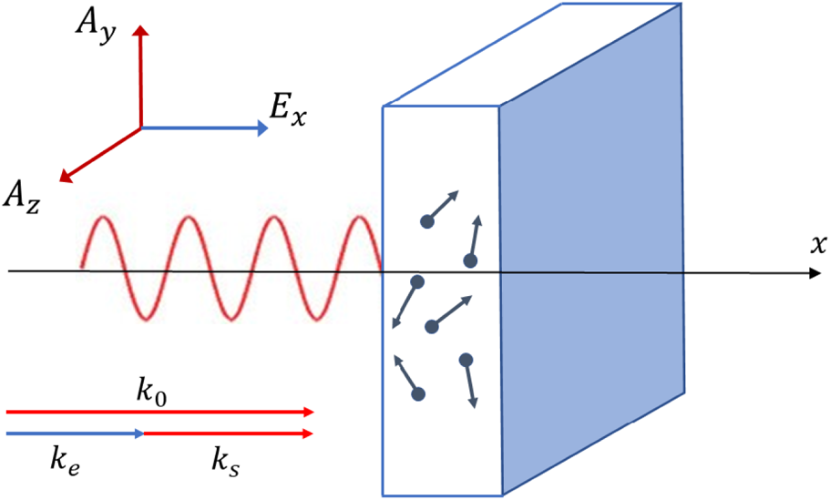
This section is dedicated to numerical simulations of the laser–plasma models presented above. Laser–plasma interactions are a broadly studied topic in plasma physics. An important problem in this field is the acceleration of charged particles by large amplitude plasma waves, which may be created, amongst others, through stimulated Raman scattering (SRS) (Forslund, Kindel & Lindman Reference Forslund, Kindel and Lindman1975). During SRS, an incident electromagnetic wave generates a scattered electromagnetic wave and a Langmuir plasma wave that accelerates the electrons (see figure 1). Here, our goal is to investigate the effect of the electron spin on the SRS instability through the simulation of the vectorial spin-Vlasov–Maxwell model (2.19) by using the grid-based (Eulerian) time-splitting method described in the preceding section.
Schematic view of the geometry of the laser–plasma interaction during stimulated Raman scattering. The electromagnetic vector potential lies in the transverse plane $(y,z)$ , whereas the electrostatic field is directed along the longitudinal direction $x$
 , which is the direction of propagation of the electromagnetic wave. Here $k_0$
 , $k_s$
 and $k_e$
 represent the wavenumbers for the incident wave, the scattered wave and the electron plasma wave, respectively.

Our analysis will proceed step by step. First, we consider the problem without spin, which has been studied in several earlier works (Ghizzo et al. Reference Ghizzo, Bertrand, Shoucri, Johnston, Fualkow and Feix1990; Huot et al. Reference Huot, Ghizzo, Bertrand, Sonnendrücker and Coulaud2003; Li et al. Reference Li, Sun and Crouseilles2020) (§ 3.1). Second, we compare the results obtained with the scalar and vector models at short times, for different values of the scaled Planck constant $\mathfrak {h}$ (§ 3.2.1). Next, we remove the effect of plasma self-consistency on the propagation of the electromagnetic wave, in order to precisely validate the numerical simulations for long times (§ 3.2.2). Finally, we simulate the general spin-dependent vector model for $\gamma =0$
 and $1$
 (which corresponds to $\alpha =1$
 and $3$
 , respectively) and check its conservation properties and other physical issues (§ 3.2.3).
3.1. Stimulated Raman Scattering without spin
We consider the model corresponding to (2.19) with $\boldsymbol {f}=0$ and ${\mathfrak h}=0$
 (which is the model studied in Ghizzo et al. Reference Ghizzo, Bertrand, Shoucri, Johnston, Fualkow and Feix1990; Li et al. Reference Li, Sun and Crouseilles2020). We use a perturbed Maxwellian as initial condition for $f_0$
 ,

and the initial longitudinal electric field $E_x(t=0,x)=(\epsilon /k_e)\sin (k_e x)$ . Here, $\epsilon$
 and $k_e$
 are the amplitude and the wavenumber of the perturbation, respectively, and $v_{{\rm th}}$
 is the electron thermal speed (normalized to $c$
 ). For the transverse fields, we consider an incident electromagnetic wave with circular polarization,

where $k_0$ , $\omega _0$
 and $E_0$
 are the wavenumber, frequency and amplitude of the transverse electric field, respectively. We consider periodic boundary conditions with spatial period $L=4{\rm \pi} /k_e$
 , and take $p_{\max }=5$
 for the computational domain in momentum space. A schematic view of the geometry is shown in figure 1.
The dispersion relation can be derived from the usual matching conditions for frequency and wavenumber,

and

where the subscript ‘$0$ ’ refers to the pump wave, ‘$s$
 ’ to the scattered electromagnetic wave and ‘$e$
 ’ to the electron plasma wave. As in Ghizzo et al. (Reference Ghizzo, Bertrand, Shoucri, Johnston, Fualkow and Feix1990), we take the following values for the above parameters:

Then, using the matching relations (3.3a,b) and (3.4a,b), we get

Finally, we take the amplitude of the incident wave $E_0=E_{{\rm ref}}=0.325$ as a reference value.
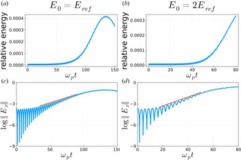
To check the accuracy of our code in the spinless regime, the grid parameters are taken as $N_x=129,\ N_p=129,\ \Delta t =0.05$ and a Strang splitting method is used for the time discretization. As we can observe in figure 2(a,b), the code preserves the total energy to very high precision (the relative error is less than $0.05\,\%$
 ).
The SRS simulations without spin. Time evolution of the relative energy $|E_{tot}(t) - E_{tot}(0)|/E_{tot}(0)$ (a,b) and of the longitudinal electric field norm $\|E_x(t)\|$
 in semilog scale (c,d), for $E_0 = E_{{\rm ref}}= 0.325$
 (a,c) and $E_0 = 2E_{{\rm ref}}= 0.65$
 (b,d). The red straight lines represent the instability growth rate expected from linear theory.

We also consider the Poisson equation conservation; to do so, we define the quantity ${\rm Poi.err}$ as

where $\hat {E}_{x,k}(t)$ is the $k$
 th Fourier component of the longitudinal electric field $E_x$
 , and $\hat {f}_{k,l}(t)$
 is the $k$
 th Fourier component of the distribution function $f(x,p,t)$
 computed at the $l$
 th grid point in momentum space. If Poisson's equation is satisfied, the above quantity should vanish. We observe, as expected, that the Poisson equation conservation is ensured at the machine precision level. In figure 2(c,d), we also plot the time evolution of the longitudinal electric field norm

in semilog scale, for two values of the incident amplitude ($E_0=E_{{\rm ref}}=0.325$ and $E_0=2E_{{\rm ref}}=0.65$
 ). We observe that the instability growth rate ($\gamma _{{\rm inst}} \approx 0.03$
 for $E_0=E_{{\rm ref}}$
 and $\gamma _{{\rm inst}} \approx 0.06$
 for $E_0=2 E_{{\rm ref}}$
 ) is proportional to the amplitude $E_0$
 and close to the value expected from the linear theory (Ghizzo et al. Reference Ghizzo, Bertrand, Shoucri, Johnston, Fualkow and Feix1990).
3.2. Vector and scalar models with spin
Here, several comparisons are performed between the vector and scalar models in different configurations, but always with $\alpha =\beta =1$ and $\gamma =0$
 . Indeed, when $\gamma \neq 0$
 the PIC code could not be used because of the double derivative in $\boldsymbol p$
 and $\boldsymbol s$
 in the Vlasov equation. We recall that the other condition ($\alpha =\beta =1$
 ) ensures the Poisson structure for the PIC method. However, as pointed out earlier, with this choice the scalar and vector models are not mathematically equivalent. Hence, any observed differences in the results may originate from either this inequivalence or from the different numerical method employed in the simulations (PIC or Eulerian).
We use the following initial conditions for the scalar model:

and for the vector model

with $x\in [0, 4{\rm \pi} /k_e],\ p \in \mathbb {R},\ \boldsymbol {s} \in {\mathbb {S}}^2$ . The variable $\eta$
 represents the degree of spin polarization of the electron gas (Manfredi et al. Reference Manfredi, Hervieux and Hurst2019): $\eta =0$
 for an unpolarized electron gas and $\eta =1$
 for a fully polarized one. In the following, we use $\eta =0.5$
 and the parameters for the electromagnetic fields are the same as in the spinless case of § 3.1 (circularly polarized wave).
We will first compare the full models for short times (§ 3.2.1), then we consider a simplified model (neglecting self-consistency) for long times (§ 3.2.2), and finally we compare results for the full models at long times (§ 3.2.3).
3.2.1. Full spin-dependent models at short times
In this part, we focus on the solutions for short times (approximately $100 \omega _p^{-1}$ ), which enables us to employ refined numerical parameters in order to compare as accurately as possible the two models.
From Proposition 1, we proved the equivalence between the scalar and vector models. However, this equivalence is only true for $\gamma \neq 0$ , so that the term $\gamma \mathfrak {h}\boldsymbol {\nabla } (\boldsymbol {B}\boldsymbol {\cdot }{\partial }/{\partial \boldsymbol {s}})\boldsymbol {\cdot } {\partial f}/{\partial \boldsymbol {p}}$
 is present in the scalar Vlasov equation (2.15). This term cannot be easily described using standard PIC methods based on trajectories, hence, it is neglected most of the time. However, when $\mathfrak {h}=0$
 this term disappears, so that the two models are again equivalent for any value of $\gamma$
 . Then, by progressively increasing $\mathfrak {h}$
 , we can show how the results of the scalar and vector models depart from each other. The numerical solutions are obtained using the PIC code described in our earlier work (Crouseilles et al. Reference Crouseilles, Hervieux, Li, Manfredi and Sun2021) and the grid-based Eulerian code presented in the preceding section of the present paper.
To control the influence of the numerical error, we use a refined mesh for both methods: $N_x=258$ and $N_p=10^3$
 for the grid-based method, and $N_x=258$
 with number of particles $N_{\textrm {part}}=10^5$
 for the PIC method. The initial conditions are given by (3.10) with $\eta =0.5, \alpha =0.02, v_{\textrm {th}}=0.17$
 and $E_0=E_{\textrm {ref}}$
 . Finally, the time step is $\Delta t =0.004$
 for both cases (both methods use a Strang splitting) and we consider the following values for the scaled Planck constant $\mathfrak {h}=0,\ 0.001,\ 0.1,\ 0.25,\ 0.5,\ 0.75$
 and $1$
 . We note that, strictly speaking, for such large values of $\mathfrak {h}$
 a relativistic treatment of the motion should be adopted. However, here the purpose is simply to study the agreement between the scalar and vector models, so that all considerations about relativistic corrections are ignored.
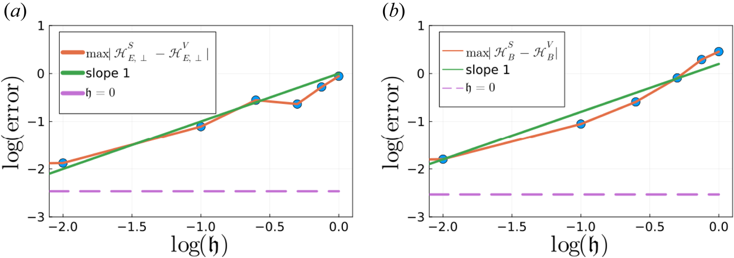
In figure 3, we study the difference (‘error’) between the scalar and vector models by considering the perpendicular electric energy $\mathcal {H}_{E,\perp }=\frac {1}{2} \int (E_y^2+E_z^2)\,\mathrm {d}x$ and the magnetic energy $\mathcal {H}_B=\frac {1}{2} \int (B_y^2+B_z^2)\,\mathrm {d}x$
 . We plot, on a log–log scale, the error (in the $L^\infty$
 norm) of these energies obtained from the scalar and vector models, for different values of $\mathfrak {h}$
 . For both energies, the difference decreases with decreasing $\mathfrak {h}$
 in an approximately linear fashion. This is in agreement with the fact that, for $\gamma =0$
 , the difference between two models is expected to be $O(\mathfrak {h})$
 . For very small values of ${\mathfrak {h}}$
 , the difference between the two models saturates to the numerical error due to the different numerical methods (PIC and Eulerian). The horizontal dashed line in figure 3 corresponds to such numerical error observed for $\mathfrak {h}=0$
 .
Difference ($L^\infty$ norm) between the scalar (superscript $S$
 ) and vector (superscript $V$
 ) models for the perpendicular electric energy ($\mathcal {H}_{E,\perp }$
 , a) and magnetic energy ($\mathcal {H}_B$
 , b), for different values of the scaled Planck constant $\mathfrak {h}$
 . The horizontal dashed lines correspond to the numerical error observed for $\mathfrak {h}=0$
 . The green straight line has a slope equal to unity.

3.2.2. Spin-dependent models without wave self-consistency at long times
Here, we study the propagation of a circularly polarized wave into a plasma that does not retroact on the wave in the transverse direction, although the self-consistency along the propagation direction is maintained through the Poisson equation (Crouseilles et al. Reference Crouseilles, Hervieux, Li, Manfredi and Sun2021). To simulate this, we consider a reduced model. Using the above notations, we remove the term $\frac {1}{2}\int _{\varOmega }|\boldsymbol {A}_\perp |^2 f_0\,\mathrm {d}x\,\mathrm {d}p$ from the Hamiltonian $\mathcal {H}$
 in (2.21), then through the Poisson bracket representation (2.22) we can derive a reduce system similar to (2.19), but without the terms $\boldsymbol {A}_\perp \boldsymbol {\cdot } ({\partial \boldsymbol {A}_\perp }/{\partial x}) ({\partial f_0}/{\partial p})$
 and $\boldsymbol {A}_\perp \boldsymbol {\cdot } ({\partial \boldsymbol {A}_\perp }/{\partial x}) ({\partial \boldsymbol {f}}/{\partial p})$
 in the Vlasov equations, and the terms $A_y \int _{\mathbb {R}} f_0 \,\mathrm {d}{p}$
 and $A_z \int _{\mathbb {R}} f_0 \,\mathrm {d}{p}$
 in the sources of the Maxwell equations. In this case, the electromagnetic wave is not coupled to the plasma and its evolution can be determined exactly by solving the corresponding Maxwell equations for $E_y$
 and $E_z$
 . In contrast, the longitudinal nonlinearity is kept in the model, hence, $E_x$
 is a solution of Poisson's equation.
We consider the initial condition (3.10) for the distribution functions and we use ${\eta =0.5,\ \alpha =0.02, v_{\textrm {th}}=0.17}$ and $\mathfrak {h}=0.00022$
 . The electromagnetic fields are initialized as in the spinless case (see § 3.1), but here we have different matching conditions for the circularly polarized wave, since the wave propagates in vacuum in this case. We still have the relation (3.3a,b) together with the following ones:

We still consider $k_0=2k_e$ , so that we obtain from the matching relations (3.3a,b) and (3.11a,b),

The amplitude of the incident wave is $E_0=E_{\textrm {ref}}=0.325$ .
Neglecting the spatial dependence and considering the following time dependent magnetic field $\boldsymbol {B}=(0,B_0\sin (\omega _0 t),-B_0\cos (\omega _0 t))$ with $B_0=E_0k_0/\omega _0$
 , one can obtain an approximate closed equation for the dynamics of the macroscopic spin ${S}_z(t)$
 (with ${S}_z(t)=\frac {1}{3}\int f_3 \,\mathrm {d}x\,\mathrm {d}p$
 for the vector case and ${S}_z(t)=\int s_3 f \,\mathrm {d}x\,\mathrm {d}p\, \mathrm {d}\boldsymbol {s}$
 for the scalar case). In the regime $B_0/\omega _0 \ll 1$
 (i.e. when the Larmor precession frequency $eB_0/m$
 is much smaller than the laser frequency), it can be shown that the spin $S_z(t)$
 oscillates with a frequency $\omega _\textrm {spin}=B_0^2/(2\omega _0)$
 (see Crouseilles et al. (Reference Crouseilles, Hervieux, Li, Manfredi and Sun2021) for more details).
On the numerical side, we use the same parameters as in § 3.1 (i.e. $N_x=N_p=129$ and $\Delta t=0.04$
 ) for the Eulerian method and $N_x=128,\ N_{\textrm {part}}=2\times 10^4,\ \Delta t=0.04$
 for the PIC method. Different values of the incident wave amplitude $E_0$
 are studied to compare the numerical results with the analytic frequency $\omega _{\textrm {spin}}=B_0^2/(2\omega _0)$
 . Indeed, as the transverse retroaction terms were removed from the Vlasov equation, we do not expect an instability here, so that the amplitude of the incident wave should remain approximately constant, which justifies the analytical calculations.
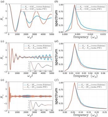
In figure 4, the time evolution of $S_z$ obtained by the vector model (Eulerian method) and scalar model (PIC method) are displayed for three values of the amplitude of the incident electromagnetic wave $E_0$
 . The corresponding spectrum, normalized to its peak value, is also shown in figure 4(b,d, f). We observe that $S_z$
 displays an oscillatory damped behaviour for all cases, with a damping rate that is significantly higher when $E_0$
 increases. The damping rate is slightly larger for the vector model at long times, but the agreement between the two approaches is very good for short times (up to ${\approx }1500 \omega _p^{-1}$
 ). In the spectrum, the expected analytical frequencies $\omega _{\textrm {spin}}= 0.0039,\ 0.0158$
 and $0.063$
 are also recovered with good precision. In particular, the quadratic scaling between $\omega _{\textrm {spin}}$
 and $B_0$
 is correctly reproduced.
Spin-dependent reduced model without wave self-consistency. Time evolution of $S_z$ (a,c,e) and frequency spectrum of $S_z$
 (b,d, f), for the scalar (red lines) and vector (blue lines) models. We recall that $S_z=\int s_3 f \,\mathrm {d}x\,\mathrm {d}p\,\mathrm {d}\boldsymbol {s}$
 for the vector model (Eulerian code) and $S_z=\frac {1}{3}\int f_3 \,\mathrm {d}x\,\mathrm {d}p$
 for the scalar model (PIC code). The amplitude of the incident wave is, from top to bottom, $E_0=0.5E_{\textrm {ref}}$
 , $E_0=E_{\textrm {ref}}$
 and $E_0=2E_{\textrm {ref}}$
 . The analytical predictions for the peak frequency are $\omega _{\textrm {spin}}= 0.0039,\ 0.0158$
 and $0.063$
 , from top to bottom.

3.2.3. Full spin-dependent models at long times
Here, we present numerical results corresponding to $\alpha =1,\ \beta =1, \gamma =0$ for the scalar and vector models for large times (the short time behaviour was investigated in § 3.2.1). In this case, the models are not equivalent as soon as $\mathfrak {h}\neq 0$
 ; however, the Poisson bracket structure is ensured for both models, so that the Hamiltonian splitting can be used (Strang splitting) to get a good total energy conservation for both codes. The initial condition for the distribution functions is that of (3.10) and the electromagnetic waves are circularly polarized, with the same parameters as in the spinless case of § 3.1.
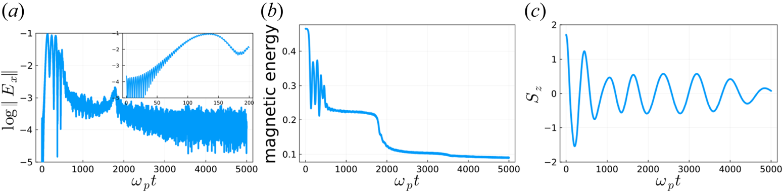
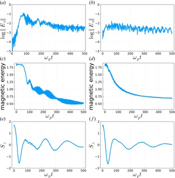
Eulerian code results (vector model). First, we illustrate the general results obtained with the Eulerian (vector approach), before proceeding to the systematic comparison with the PIC code (scalar approach). The results, which were obtained with $\mathfrak {h}=0.00022$ , are shown in figures 5 and 6.
Full spin-dependent vector model (Eulerian method with $N_x=259, N_p=512,\ p\in [-2.5,2.5],\ \Delta t=0.02$ ). (a) Longitudinal electric field norm $\|E_x \|$
 in semilog scale (the inset shows a zoom on short times to highlight the linear instability phase with slope ${\approx }0.03$
 ). (b) Magnetic energy $\frac {1}{2}\int |\boldsymbol {B}|^2\,\mathrm {d}x$
 . (c) Spin component ${S}_z(t)$
 .

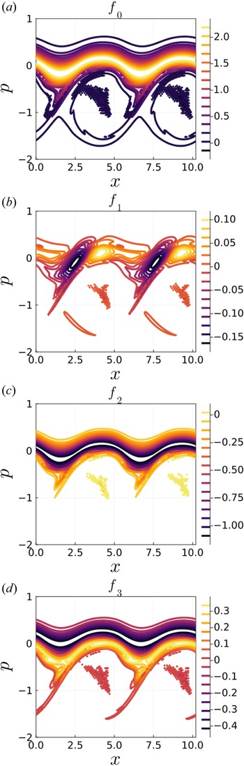
Full spin-dependent vector model (Eulerian method with $N_x=129, N_p=256,\ p\in [-2.5,2.5],\ \Delta t=0.04$ ). From (a) to (d): contour plots of the four components of the electron distribution function $f_0$
 , $f_1$
 , $f_2$
 , $f_3$
 in the phase space $(x,p)$
 , at time $t=320 \omega _p^{-1}$
 .

The instability rate measured from the growth of the longitudinal electric field amplitude $\|E_x(t)\|$ is close to the one observed in the spinless simulations ($\gamma _{\textrm {inst}} \approx 0.03$
 ). Moreover, the magnetic field energy strongly decreases during the linear phase (where the longitudinal electric energy increases exponentially) to reach a plateau, before another strong drop around $t\approx 2000 \omega _p^{-1}$
 . Finally, the spin component ${S}_z(t)= \frac {1}{3}\int f_3 \,\mathrm {d}x\,\mathrm {d}p$
 has a damped oscillatory behaviour which is qualitatively similar to the results obtained with the PIC approach (Crouseilles et al. Reference Crouseilles, Hervieux, Li, Manfredi and Sun2021).
We also show, in figure 6, the phase space portraits of the distribution functions $f_0, f_1, f_2, f_3$ at time $t=320\omega _p^{-1}$
 . Two phase-space vortices can be clearly seen in these figures thanks to the high-order numerical methods used for these Eulerian simulations. As expected, the size of each vortex is close to the wavelength of the unstable plasma wave $2{\rm \pi} /k_e \approx 5.15$
 (see § 3.1). We note that the statistical noise inherent to PIC codes would have precluded such high-resolution diagnostics.
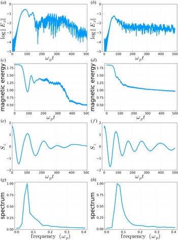
Comparison with PIC code (scalar model) for $\mathfrak {h}=0$ . In figure 7, we compare the vector and scalar models with $E_0=2E_{\textrm {ref}}$
 and $\mathfrak {h}=0$
 . When $\mathfrak {h}=0$
 and $\alpha =\beta =1,\ \gamma =0$
 , the scalar and vector models are mathematically equivalent, but the results may differ because of the different numerical methods that are used. Therefore, this is a good comparative test of the two numerical methods.
Comparison of the full spin-dependent vector and scalar models with $\mathfrak {h}=0.0$ and $E_0=2 E_{\textrm {ref}}$
 (Eulerian method with $p\in [-5,5]$
 $N_x=259,\ N_p= 512,\ \Delta t=0.02$
 and PIC method with $N_x=259,\ N_{\textrm {part}}= 10^5,\ \Delta t=0.02$
 ). (a,c,e,g) Vector model with Eulerian method; (b,d, f,h) scalar model with PIC method. From top to bottom are shown (a,b) the longitudinal electric field, (c,d) the magnetic energy, (e, f) the spin component $S_z$
 , and (g,h) its frequency spectrum.

First, we observe that the instability rate on $\|E_x(t)\|$ is similar for the two approaches, and very close to the one observed in the spinless case ($\gamma _\textrm {inst}\approx 0.06$
 ). We also checked that the growth rate is linear with respect to $E_0$
 by running the case $E_0=E_{\textrm {ref}}$
 (twice as small as in figure 7) and that the total energy is very well conserved (with an error ${\approx }10^{-5}$
 even for long times, for both codes). Second, we can see that the spin frequencies obtained from the PIC and Eulerian simulations are very similar (${\approx }0.08\omega _p$
 ).
Generally speaking, the results of the two codes are in good agreement, particularly during the initial linear phase. The remaining observed differences should be attributed to the two numerical methods (PIC and Eulerian), which are intrinsically different in their approaches.
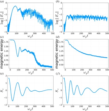
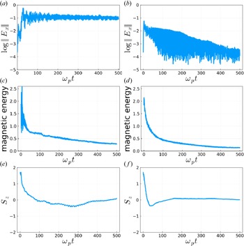
Effect of the scaled Planck constant. In figures 8, 9 and 10, the influence of $\mathfrak {h}$ ($\mathfrak {h}=0.01, 0.1$
 and $0.5$
 ) is studied for the vector and scalar models for $E_0=2E_{\textrm {ref}}$
 . The same initial condition as before is used and $\alpha =\beta =1,\ \gamma =0$
 . Let us recall that here, since $\mathfrak {h}\neq 0$
 , the two models are not mathematically equivalent. The linear phase becomes quite different as $\mathfrak {h}$
 increases: in particular, the electric energies do not saturate at the same level. However, the evolution of ${S}_z$
 is similar for both approaches: the oscillations are damped more quickly as $\mathfrak {h}$
 increases. For both codes, the total energy is well preserved (the relative error is approximately $10^{-4}$
 , not shown). Finally, the magnetic energies, even though they both decrease in the two approaches, have rather different behaviours, with a bigger drop observed for the vector model. Of course, the differences can be explained by the fact that in this case the underlying models are not equivalent. We emphasize that the Eulerian code has been tested on several meshes to ensure the numerical convergence, whereas the PIC code would require, in order to achieve convergence, a large number of particles $N_p$
 that would lead to very time-consuming simulations.
Comparison of the full spin-dependent vector and scalar models for $\mathfrak {h}=0.01$ and $E_0=2E_{\textrm {ref}}$
 (Eulerian method with $p\in [-5,5]$
 $N_x=259,\ N_p= 512,\ \Delta t=0.02$
 and PIC method with $N_x=259,\ N_{\textrm {part}}= 10^5,\ \Delta t=0.02$
 ). (a,c,e) Vector model with Eulerian method; (b,d, f) scalar model with PIC method. From top to bottom, we show (a,b) the time evolution of the longitudinal electric field, (c,d) the magnetic energy, and (e, f) the spin component $S_z$
 .

Same as figure 8 for $\mathfrak {h}=0.1$ .

Same as figure 8 for $\mathfrak {h}=0.5$ .

Finally, we note, by comparing figures 8(e, f), 9(e,f) and 10(e, f), that the spin oscillations are more strongly damped for larger values of $\mathfrak {h}$ .
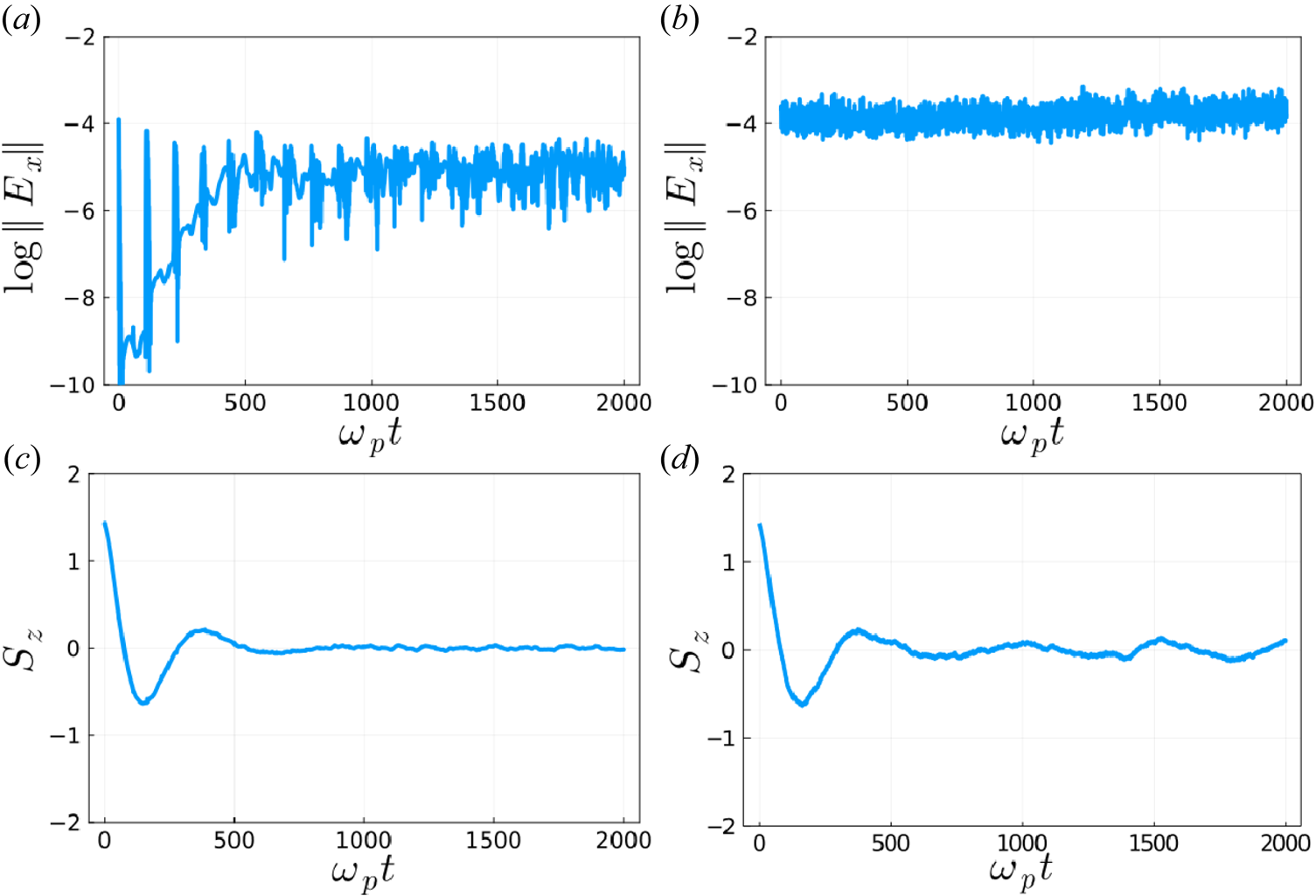
Temperature effects. In figure 11, we study the influence of a higher electron temperature by taking $v_{\textrm {th}}=0.51$ in the initial condition (3.10) for the Eulerian and PIC codes (instead of $v_{\textrm {th}}=0.17$
 in figure 5). The field amplitude is fixed to $E_0=E_{\textrm {ref}}$
 and $\mathfrak {h}=0.00022$
 . For the present case $v_{\textrm {th}}=0.51$
 , the matching relations (3.3a,b) and (3.4a,b) yield the wavenumbers $k_e=1.46$
 and $k_0=2k_e$
 . In figure 11, we show the time evolution of the electric energy and the spin component ${S}_z$
 for the Eulerian and PIC methods. These results have to be compared with the case $v_{\textrm {th}}=0.17$
 presented in figure 5.
Influence of the electron temperature using $v_{\textrm {th}}=0.51$ . (a,b) Time evolution of the electric energy (semilog scale). (c,d) Time evolution of the spin $S_z$
 . (a,c) Full spin-dependent vector model (Eulerian method with $N_x=N_p=129,\ \Delta t=0.04$
 ). (b,d) Full spin-dependent scalar model (PIC method with $N_x=129,\ N_{\textrm {part}}=2\times 10^4,\ \Delta t=0.04$
 ).

Thanks to its superior resolution, the Eulerian code allows the initial longitudinal electric field to be very small (figure 11a), in accordance with the initial condition (3.10). Subsequently, this initial perturbation grows unstable and saturates nonlinerarly at a certain (still rather small) value. The spikes observed on the figure correspond to the well-known recurrences occurring at times multiple of $2{\rm \pi} /(k_e \Delta p)$ , where $\Delta p$
 is the grid step in momentum space. These recurrences are due to the discretization of momentum space. In contrast, the PIC code (figure 11b) cannot resolve the initial small perturbation because of its inherent noise, so the instability is lost. Indeed, the noise level of the PIC code is even higher than the saturation level observed for the Eulerian code.
In spite of these limitations, the spin component $S_z$ decreases in a similar fashion for both methods, and becomes almost zero after $\omega _p t=1000$
 .
By comparing the results of figure 11 ($v_{\textrm {th}}=0.17$ ) and figure 5 ($v_{\textrm {th}}=0.51$
 ), we also note that the spin component $S_z$
 is more strongly damped for the case at higher temperature, as should be expected.
Full vector model with $\gamma \neq 0$ . In this last part, we simulate the full spin-Vlasov–Maxwell vector model introduced in Hurst et al. (Reference Hurst, Morandi, Manfredi and Hervieux2014, Reference Hurst, Morandi, Manfredi and Hervieux2017) and Manfredi et al. (Reference Manfredi, Hervieux and Crouseilles2022), i.e. for $\gamma =1,\alpha =3,\beta =1$
 , for which we cannot perform simulations for the scalar model, since the cross-derivative term is not implemented in our PIC code. In particular, we compare the results of the Eulerian code for this set of parameters (with $\gamma \neq 0$
 ) with those obtained with the same code but $\gamma = 0$
 and $\alpha =\beta =1$
 (see figure 9).
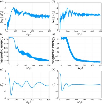
In figure 12, we show the comparison for a typical case with $E_0=2E_{\textrm {ref}}$ and $\mathfrak {h}=0.1$
 . The results are in reasonable agreement: in particular, the longitudinal electric fields and the magnetic energies saturate nonlinearly at similar levels. The $z$
 component of the spin appears to decay faster and with fewer oscillations in the $\gamma \neq 0$
 case. For both cases, the total energy is very well preserved (around $10^{-4}$
 , not shown).
Eulerian method for the vector model with $\alpha =\beta =1, \gamma =0$ (a,c,e) and ${\alpha =3,\beta =\gamma =1}$
 (b,d, f) with $\mathfrak {h}=0.1$
 . $N_x=259, N_p=10^3,\ \Delta t=0.02$
 , $E_0=2E_{\textrm {ref}}$
 . From top to bottom, we show (a,b) the norm of the longitudinal electric field, (c,d) the magnetic energy, and (e, f) the $z$
 component of the spin.

4. Conclusion
Here, we implemented and analysed the results of an Eulerian code that solves the self-consistent Vlasov–Maxwell equations for particles with spin 1/2. In this case, the phase-space distribution function has actually four components, which can be rearranged as one scalar and one vector distribution. This model was termed ‘vectorial model’ in the present work. We also compared the results with those obtained (using a PIC code) with a fully scalar model in an extended phase space that includes the spin variable – see our recent work (Crouseilles et al. Reference Crouseilles, Hervieux, Li, Manfredi and Sun2021).
In order to make systematic comparisons, we appended some artificial coefficients, $\alpha$ , $\beta$
 and $\gamma$
 to the equations, and checked the equivalence between the scalar and vector models. In particular, the scalar model includes a peculiar term that contains a double derivative in the momentum and spin variables. Due to this term, it is impossible to write the Vlasov equation in characteristic form, and, hence, to use a standard PIC code base on particle trajectories. Therefore, this term was neglected in earlier simulations (Crouseilles et al. Reference Crouseilles, Hervieux, Li, Manfredi and Sun2021), which amounts to taking $\gamma =0$
 in our notation. However, we stress that this is a quantum term, and its absence may bring into question the fully quantum nature of the scalar model, see Zamanian et al. (Reference Zamanian, Marklund and Brodin2010) for a discussion on this point.
A second issue is the existence of a Poisson structure, which is important to construct efficient numerical methods that preserve the Hamiltonian structure of the equations (Kraus et al. Reference Kraus, Kormann, Morrison and Sonnendrücker2017) and, hence, avoid numerical dissipation. For the scalar model with $\gamma =0$ , a non-canonical Poisson structure exists when $\alpha =\beta$
 , which was used in our earlier work using a PIC code (Crouseilles et al. Reference Crouseilles, Hervieux, Li, Manfredi and Sun2021). For the vector model, the structure exists when $\alpha = \beta + 2 \gamma$
 , which reduces to the same relationship as for the scalar model when $\gamma =0$
 .
Therefore, we compared systematically the two approaches in the case $\alpha =\beta =1$ and $\gamma =0$
 , for a standard plasma problem, namely the Raman instability. However, it must be stressed that the two models are not mathematically equivalent in this case, so that the observed discrepancies may come from either the models themselves or from the different numerical methods. Moreover, in the classical limit $\mathfrak {h}=0$
 , the scalar and vector models are again equivalent (because the double-derivative term is a quantum one, as pointed out above), so in this case a meaningful test of the two codes was possible. The results were encouraging, particularly on the initial linear phase of the Raman instability and on the damping of the spin amplitude. Comparisons for $\mathfrak {h} > 0$
 also showed a reasonable accordance between the two approaches, and revealed that the discrepancies progressively disappear with decreasing scaled Planck constant, as expected.
For the full model ($\gamma =1$ ) it is not possible to use the PIC code because of the double derivative problem. Hence, we compared results obtained with the vector model and the Eulerian code for the cases $\gamma =0$
 and $\gamma =1$
 . Even though the behaviour is similar, we observed that the spin is damped faster in the case $\gamma =1$
 .
In summary, the Eulerian code described here is able to simulate the quantum dynamics of a spin polarized electron plasma. Contrarily to the scalar model, no simplifications need to be made to implement the corresponding numerical code. Hence, the dynamics is fully quantum, at least for the spin variable, whereas, as usual, the orbital motion is treated classically. In addition, the well-known high-resolution properties of grid-based Eulerian codes outperform their PIC counterparts in many respects, particularly for subtle effects that occur at low particle density, such as the formation of phase-space vortices. The present Eulerian code is thus a valuable tool for further studies in this domain.
Acknowledgements
The work was supported by the Centre Henri Lebesgue (N.C., X.H., project ANR-11-LABX-0020-0); and by the Brittany Council (N.C., X.H.). We also thank Professor G. Brodin and Dr J. Zamanian for several useful discussions on the equivalence between the scalar and vector models.
Editor A.C. Bret thanks the referees for their advice in evaluating this article.
Declaration of interests
The authors report no conflict of interest.
Appendix A. Proof of Proposition 1
First of all, we give some calculations concerning the spherical coordinates transformation,

Now, assuming that the initial condition satisfies $f(t=0) = ({1}/{4{\rm \pi} }) (f_0(t=0) + \boldsymbol {s}\boldsymbol {\cdot } \boldsymbol {f}(t=0))$ , we check that $f(t) =({1}/{4{\rm \pi} })(f_0(t)+{\boldsymbol {s}}\boldsymbol {\cdot }{\boldsymbol {f}}(t))=({1}/{4{\rm \pi} })(f_0(t)+\sum _i s_if_i(t))$
 is true for all times $t>0$
 . To do so, we insert the decomposition $f(t) =({1}/{4{\rm \pi} })(f_0(t)+{\boldsymbol {s}}\boldsymbol {\cdot }{\boldsymbol {f}}(t))$
 into the scalar equation (2.2). Of course, the terms $\partial f/\partial t, \boldsymbol {p}\boldsymbol {\cdot }\boldsymbol {\nabla } f$
 and $[\boldsymbol {E}+\boldsymbol {p}\times \boldsymbol {B}]\boldsymbol {\cdot } \partial f/\partial \boldsymbol {p}$
 satisfy this property. Let us focus on the other terms $(\boldsymbol {s}\times \boldsymbol {B}) \boldsymbol {\cdot } \partial f/\partial \boldsymbol {s},\ \mathfrak {h} \boldsymbol {\nabla }(\boldsymbol {s}\boldsymbol {\cdot } \boldsymbol {B}) \boldsymbol {\cdot } \partial f/\partial \boldsymbol {p}$
 and $\mathfrak {h} \boldsymbol {\nabla } (\boldsymbol {B}\boldsymbol {\cdot } {\partial }/{\partial \boldsymbol {s}})\boldsymbol {\cdot } \partial f/\partial \boldsymbol {p}$
 by using the relations (A1).
For the first term, we have

Regarding the second term ${\beta }\mathfrak {h} \boldsymbol {\nabla }(\boldsymbol {s}\boldsymbol {\cdot } \boldsymbol {B}) \boldsymbol {\cdot } \partial f/\partial \boldsymbol {p}$ , we have

Finally, the third term $\gamma \mathfrak {h} \boldsymbol {\nabla } (\boldsymbol {B}\boldsymbol {\cdot }{\partial }/{\partial \boldsymbol {s}}) \boldsymbol {\cdot } \partial f/\partial \boldsymbol {p}$ becomes

Then, adding the contributions of these last three terms, we observe that the quadratic terms cancel out for $\beta =\gamma$ and we finally get for this case

Gathering all the terms of the scalar equation enables us to get

Since $(1, s_1, s_2, s_3)$ is a basis, we can identify the coefficients to be zero, which leads to the four equations of the vector model satisfied by $(f_0, f_1, f_2, f_3)$
 . Thus, since $f$
 and $({1}/{4{\rm \pi} })(f_0+{\boldsymbol {s}}\boldsymbol {\cdot }{\boldsymbol {f}})$
 share the same initial condition, we get that $f=({1}/{4{\rm \pi} })(f_0+{\boldsymbol {s}}\boldsymbol {\cdot }{\boldsymbol {f}})$
 is a solution of the scalar model if and only if $(f_0,f_1,f_2,f_3)$
 is the solution of vector model (2.8).
Appendix B. Derivation of the 1-D vector model (Proposition 2)
To derive the vector model from the scalar one in the laser–plasma context considered in the main text, we will take the moments with respect to the variable $\boldsymbol {s}$ of the scalar model (2.15). Thus, we first multiply (2.15) by $(1,3\boldsymbol {s})$
 , thus integrate with respect to $\boldsymbol {s}$
 and finally, use the representation

We shall use the following identities which can be calculated from the spherical coordinates transformation using (B1):

We integrate the first equation in (2.15) with respect to $\boldsymbol {{s}}$ on $\mathbb {S}^2$
 and use (B1) and (B2) to get the following equation on $f_0$
 :

With our magnetic field $(\boldsymbol {B}=(0, -\partial _x A_z, \partial _x A_y))$ , this equation can be reformulated as

Thus, we multiply the first equation in (2.15) multiplied by $3 \boldsymbol {s}$ , integrate with respect to $\boldsymbol {s}$
 on $\mathbb {R}^3$
 and use (B1) to get the equations on $\boldsymbol {f=(f_1, f_2, f_3)}$
 . Let us detail the calculations to derive the equation on $f_1$
 . First, multiplying (2.15) by $3 s_1$
 and integrating with respect to $\boldsymbol {{s}}$
 leads to the following equation for $f_1$
 :

Using the relations (B1) and (B2), we get that terms one and two are equal to zero, term three is equal to $-f_3/5$ , term four is equal to $-f_2/5$
 , term five is equal to $-4f_2/5$
 , term six is equal to $-4f_3/5$
 . Finally, we get the following equation for $f_1$
 :

Similar calculations lead to the equations for $f_2$ and $f_3$
 . Using the vector notation $\boldsymbol {f=(f_1, f_2, f_3)}$
 , the vector system satisfied by $\boldsymbol {f}$
 can be reformulated as

It remains to be considered the coupling with the Maxwell equations, which involves integral with respect to ${\boldsymbol {s}}$ and $p$
 of the scalar unknown $f$
 . The Ampère equation simply becomes

whereas the equations on $E_y$ and $E_z$
 can be rewritten as function of $\boldsymbol {f}$
 , recalling that $f_j = 3 \int _{\mathbb {S}^2} s_j f, \,\mathrm {d}\boldsymbol {s}$


Appendix C. Solution of the subsystems involved in the Hamiltonian splitting
In this appendix, we detail the calculations of the solution of the five subsystems involved in the splitting, as described in § 2.3.
C.1. Subsystem for $\mathcal {H}_p$

The subsystem ${\partial \mathcal {Z}}/{\partial t} = \{\mathcal {Z}, \mathcal {H}_p \}$ associated with $\mathcal {H}_{p} = \frac {1}{2}\int p^2 f_0 \,\mathrm {d}{x}\,\mathrm {d}{p}$
 is

We denote the initial datum as $(f_0^0(x,p),\boldsymbol {f}^0(x,p), E_x^0(x),\boldsymbol {E}_\perp ^0(x),\boldsymbol {A}_\perp ^0(x))$ at time $t=0$
 . The solution at time $t$
 of this subsystem can be written explicitly as

Next, we check that this solution correctly propagates the Poisson equation. To do so, we assume that the Poisson equation holds initially, i.e. ${\partial E_x^0}/{\partial x}=\int _{\mathbb {R}} f_0^0\,\mathrm {d}{p}-1$ . Then we have, by differentiating the expression of $E_x(t, x)$
 with respect to $x$
 ,

which proves that the Poisson equation is satisfied at time $t$ .
C.2. Subsystem for $\mathcal {H}_A$

The subsystem ${\partial \mathcal {Z}}/{\partial t} = \{\mathcal {Z}, \mathcal {H}_A \}$ associated with the subhamiltonian $\mathcal {H}_{A} = \frac {1}{2}\int |\boldsymbol {A}_\perp |^2 f_0 \,\mathrm {d}\boldsymbol {x} \mathrm {d}{p}+\frac {1}{2}\int |{\partial \boldsymbol {A}_\perp }/{\partial x}|^2\,\mathrm {d}{x}$
 is

We denote by $(f_0^0(x,p),\boldsymbol {f}^0(x,p), E_x^0(x),\boldsymbol {E}_\perp ^0(x),\boldsymbol {A}_\perp ^0(x))$ the initial value at time $t=0$
 . The exact solution at time $t$
 is

Let us remark that the third equation uses the fact that $\int _{\mathbb {R}} f_0(x,p,t)\,\mathrm {d}p=\int _{\mathbb {R}} f_0^0(x,p) \,\mathrm {d}p$ , which can be obtained by integrating the first of (C4) with respect to $p$
 , i.e. $\partial _t (\int _{\mathbb {R}} f_0(x,p,t)\,\mathrm {d}p) = 0$
 .
C.3. Subsystem for $\mathcal {H}_E$

The subsystem ${\partial \mathcal {Z}}/{\partial t} = \{\mathcal {Z}, \mathcal {H}_E\}$ associated with the subhamiltonian $\mathcal {H}_{E} = \frac {1}{2}\int |\boldsymbol {E}|^2 \,\mathrm {d}{x}$
 is

With the initial value $(f_0^0(x,p),\boldsymbol {f}^0(x,p),E_x^0(x),\boldsymbol {E}_\perp ^0(x),\boldsymbol {A}_\perp ^0(x))$ at time $t=0$
 , the solution at time $t$
 is as follows:

C.4. Subsystem for $\mathcal {H}_2$

The subsystem ${\partial \mathcal {Z}}/{\partial t} = \{ \mathcal {Z}, \mathcal {H}_2 \}$ associated with the subhamiltonian $\mathcal {H}_{2} = ({\alpha \mathfrak {h}}/{3}) \int f_2 ({\partial A_z}/{\partial x}) \,\mathrm {d}x\,\mathrm {d}p$
 is

In this subsystem, we observe some coupling between the distribution functions. To write down the exact solution, we reformulate the equations for $(f_0, \boldsymbol {f})$ , using $A_z(x, t)=A_z^0(x)$
 , as follows:

where $J$ denotes the symplectic matrix

With the initial data $(f_0^0(x,p),\boldsymbol {f}^0(x,p),E_x^0(x),\boldsymbol {E}_\perp ^0(x),\boldsymbol {A}_\perp ^0(x))$ at time $t=0$
 , the exact solution for the first system is

Let us now focus on the second system

By the eigen-decomposition (to simplify, we assume $\alpha > 0,\ \beta > 0$ here)

then, one can diagonalize the transport equation to get

Finally, we can solve the transport equation

and compute the exact solution at time $t$ as follows:

The last equation can easily obtained by verifying that $\int _{\mathbb {R}} f_2(x, p, t)\,\mathrm {d}{p} = \int _{\mathbb {R}} f^0_2(x, p, t)\,\mathrm {d}{p}$ .
C.5. Subsystem for $\mathcal {H}_3$

The subsystem ${\partial \mathcal {Z}}/{\partial t} = \{\mathcal {Z}, \mathcal {H}_3\}$ associated with the subhamiltonian $\mathcal {H}_{3} = -\int _{\varOmega } ({\alpha \mathfrak {h}}/{3}) f_3 ({\partial A_y}/{\partial x})\,\mathrm {d}x\,\mathrm {d}p$
 is

This subsystem is very similar to the $\mathcal {H}_2$ one, hence, as previously, we reformulate the equations on the distribution functions as

with initial data $(f_0^0(x,p),\boldsymbol {f}^0(x,p),E_x^0(x),\boldsymbol {E}_\perp ^0(x),\boldsymbol {A}_\perp ^0(x))$ at time $t=0$
 . We derive similar formulae with $\mathcal {H}_2$
 for the exact solution at time $t$


To compute the solution $E_y(x,t)$ , we use the fact that $\int _{\mathbb {R}} f_3(x,p,t)\,\mathrm {d}p =\int _{\mathbb {R}} f_3^0(x,p)\mathrm {d} p$
 .
C.6. Fully discrete numerical scheme
Finally, we consider the phase space and time discretization to get the full discretization for above vectorial model.
We assume that the computational domain is $[0,L]\times [-p_{\max }, p_{\max }]$ for $x$
 and $p$
 . The system is periodic in the $x$
 direction with period $L$
 and has compact support on $[-p_{\max }, p_{\max }]$
 in $p$
 direction. The mesh is as follows:


C.6.1. Phase space representation
Here we use the same discretization method as in Li et al. (Reference Li, Sun and Crouseilles2020). We first present the spatial discretization of $E_x$ in detail, the same strategy can be used to $\boldsymbol {E}_\perp$
 and $\boldsymbol {A}_\perp$
 . Denoting $E_{x,j}=E_x(x_j,t)$
 , we use the spectral Fourier expansion to approximate $E_x$
 as it is periodic in the $x$
 direction,

For the distribution functions $(f_0, \boldsymbol {f})$ , we use a spectral Fourier expansion for the $x$
 direction and a finite-volume method for the $p$
 direction. For simplicity, we only show the representation for $f_0$
 , the notations for $\boldsymbol {f}$
 being the same. Here $f_{0,j,\ell }(t)$
 denotes the average of $f_0(x_j,p,t)$
 over a cell $C_\ell =[p_{\ell -1/2}, p_{l+1/2}]$
 with the midpoint $p_{\ell -1/2}=(\ell -1/2)\Delta p-P_L$
 , that is

and also by Fourier expansion in $x$ direction, then

To evaluate the value of $f_0$ off-grid in $p$
 direction, we need to reconstruct a continuous function by using the cell average quantity $f_{0,j,\ell }$
 . We refer to Crouseilles, Mehrenberger & Sonnendrücker (Reference Crouseilles, Mehrenberger and Sonnendrücker2010) and Zerroukat, Wood & Staniforth (Reference Zerroukat, Wood and Staniforth2006) for a presentation of the parabolic spline method to construct a second-order polynomial approximation. To present the main idea, we consider a linear advection problem in the $p$
 direction

From the conservation of the volume, we have the following identity:

For simplicity, we denote $q\in [1, N_p]$ the index such that $p_{\ell +1/2}-at\in [p_{q-1/2},p_{q+1/2}]$
 i.e. $p_{\ell +1/2}-at \in C_q$
 , then we have

Here, we need to reconstruct a polynomial function $f(x_j,p,0)$ using the averages $f_{j,l}(0)$
 with the parabolic spline method approach. The full discretization of the different subsystems uses the tools described in Li et al. (Reference Li, Sun and Crouseilles2020).