2.1 Properties of the flow induced by wave breaking

Consider a unidirectional wave group that propagates in the $x$ direction, with $y$ denoting the transverse direction and $z$ pointed upwards. Our system is governed by the Navier–Stokes equation,

where $\boldsymbol{g}=-g\hat{\boldsymbol{z}}$ ( $\hat{\boldsymbol{z}}$ denotes the unit vector in the vertical direction) is the acceleration due to gravity, $\unicode[STIX]{x1D70C}$ the density of water and $\unicode[STIX]{x1D708}$ the fluid viscosity.

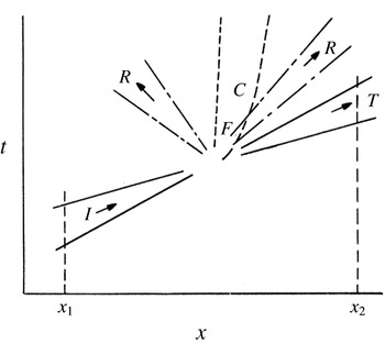
A conspicuous feature of the focusing wave packets sketched in figure 1 is that there is a natural separation between the waves and the breaking-induced flow. We will exploit this fact by forming integral relationships for the properties of the waves and the induced flow that obey simple sum relationships. That is, the waves rapidly propagate out of the region of breaking, so that we assume there is no subsequent interaction between them and the induced flow. Furthermore, we assume that any permanent exchange of momentum and energy from the wave field to the water column is confined to the region of breaking.

Figure 1.

A schematic of the focusing wave groups considered in this paper, from Rapp & Melville (Reference Rapp and Melville1990). The incident wave group, $I$ , focuses at $F$ , radiating, $R$ , and transmitting, $T$ , waves away from this region. In the area of breaking, currents, $C$ , and turbulence will be generated. Far upstream and downstream of the breaking region, $(x_{1},x_{2})$ respectively, the waves are approximately linear.

First, we consider the energy balance. To this end, we take the inner product of $\boldsymbol{u}$ with (2.1) and integrate over a control volume $V$ and time ${\mathcal{T}}_{0}$ . The control volume $V$ (with a boundary denoted as ${\mathcal{A}}$ ) is chosen so that all of the effects that we are describing, due to breaking, occur well within this domain. In particular, we integrate over a depth $(-\infty ,\unicode[STIX]{x1D702})$ and a horizontal domain $(\boldsymbol{x}_{1},\boldsymbol{x}_{2})$ . The horizontal domain is chosen so that the wave field is linear at the locations $x_{1}$ and $x_{2}$ , and the transverse direction has a range from $(-\unicode[STIX]{x1D6EC}/2,\unicode[STIX]{x1D6EC}/2)$ , where $\unicode[STIX]{x1D6EC}$ is the scale of the wave in the transverse direction. Note, the dispersive focusing laboratory experiments discussed in this paper are quasi two-dimensional, which corresponds to $\unicode[STIX]{x1D6EC}\rightarrow \infty$ . Furthermore, the (turbulent and mean) flow generated by breaking are bound to this region and do not transport integral quantities out of this volume.

Therefore, we find (Phillips Reference Phillips1977; Mei Reference Mei1989; Rapp & Melville Reference Rapp and Melville1990)

where $\boldsymbol{n}$ is a unit vector normal to the surface ${\mathcal{A}}$ , $\unicode[STIX]{x1D716}$ is the rate of dissipation and Einstein summation over repeated indices is employed.

Now, at times $t=0$ and $t={\mathcal{T}}_{0}$ , there are no waves or turbulence (following laboratory experiments (Rapp & Melville Reference Rapp and Melville1990; Melville et al. Reference Melville, Veron and White2002; Drazen & Melville Reference Drazen and Melville2009) where we have assumed that the remaining energy, several wave periods after breaking, is contained entirely in the mean vortex flow) in the volume  $V$ . Therefore, we find $(u_{i}u_{i})|_{t=0}^{t={\mathcal{T}}_{0}}=\overline{\boldsymbol{u}}({\mathcal{T}}_{0})\boldsymbol{\cdot }\overline{\boldsymbol{u}}({\mathcal{T}}_{0})$ with $\overline{\boldsymbol{u}}$ denoting the mean flow current. Furthermore, as the flow induced by breaking is confined to the interior of $V$ , the flux term will be solely due to the waves. Finally, we average over the wave period  $T$ (we denote this average by angled brackets), and conclude

where ${\mathcal{E}}_{c}$ is the (averaged) energy in the mean flow, defined as

while $\unicode[STIX]{x0394}{\mathcal{F}}={\mathcal{F}}(x_{2})-{\mathcal{F}}(x_{1})$ is the long time integrated change in energy flux, given by

and the dissipation ${\mathcal{D}}$ is given by

In this paper we will examine the ratio of ${\mathcal{E}}_{c}$ and $|\unicode[STIX]{x0394}{\mathcal{F}}|$ , which will serve to compare the energy in the mean flow to the total energy lost by the wave packet. In order to do so, we must quantify the energy in the mean flow as a function of the variables characterizing the breaking wave field.

To this end, we next perform a control volume analysis of the momentum budget. Analogous to our energy budget, we integrate the $x$ -component of equation (2.1) over the region $V$ , and over a duration ${\mathcal{T}}_{0}$ , to find

where $\unicode[STIX]{x0394}{\mathcal{S}}={\mathcal{S}}(x_{2})-{\mathcal{S}}(x_{1})$ is the long time integrated momentum flux (or radiation stress), and is given by

Recall, the velocity $\boldsymbol{u}$ remaining in $V$ at time ${\mathcal{T}}_{0}$ is solely due to the mean flow induced by breaking, i.e.  $\boldsymbol{u}=\overline{\boldsymbol{u}}$ . The second term in (2.7) is due to changes in the momentum flux of the wave groups, and has a simple solution for linear waves (Longuet-Higgins & Stewart Reference Longuet-Higgins and Stewart1964; Phillips Reference Phillips1977). Note, this quantity is in general non-zero for wave groups, unlike the wave momentum (Longuet-Higgins & Stewart Reference Longuet-Higgins and Stewart1964; McIntyre Reference McIntyre1981).

Next, based on the laboratory experiments, we assume that the momentum flux lost by the wave field goes entirely into the mean flow. That is, although some of the momentum lost from the wave field due to breaking will propagate away from the region in the form of surface waves, Rapp & Melville (Reference Rapp and Melville1990) found that the energy in these radiated waves was much less than the total energy lost by breaking. Therefore, for now we ignore this effect.

Our integral momentum balance becomes

Now, as these waves are linear at locations $x_{1}$ and $x_{2}$ , we can easily compute the integrals given in terms of the wave energy. From Longuet-Higgins & Stewart (Reference Longuet-Higgins and Stewart1964), we have ${\mathcal{S}}(x_{i})=F(x_{i})/2c_{gi}$ where the group velocity $c_{g}=\unicode[STIX]{x1D714}/2k$ for $\unicode[STIX]{x1D714}$ the angular frequency and $k$ the wavenumber. Following Drazen et al. (Reference Drazen, Melville and Lenain2008, see also Pizzo & Melville (Reference Pizzo and Melville2016)), we assume that $c_{g}\equiv c_{g}(x_{2})=c_{g}(x_{1})(1+O(S))$ , where we recall $S$ is the linear prediction of the maximum slope at breaking. This was found to be experimentally true to within 5 %–10 % (see § 3.1.1 Tian, Perlin & Choi Reference Tian, Perlin and Choi2011). Therefore, we have $|\unicode[STIX]{x0394}{\mathcal{S}}|=|\unicode[STIX]{x0394}{\mathcal{F}}|/2c_{g}$ , from which we arrive at our integral momentum balance

To make further progress, we now constrain the form of the flow induced by breaking.

2.2 A model for the mean flow induced by breaking

Consider the impulse associated with the vorticity induced by breaking, $\unicode[STIX]{x1D734}=\unicode[STIX]{x1D735}\times \overline{\boldsymbol{u}}$ . The hydrodynamic impulse, $\boldsymbol{I}$ , sometimes referred to as Kelvin’s impulse (Lamb Reference Lamb1932; Bühler Reference Bühler2007), is defined as

Note, unlike the momentum of the fluid, the impulse is well defined, as it does not contain the surface integral pressure terms which are not absolutely convergent (Batchelor Reference Batchelor1967; Saffman Reference Saffman1992; Bühler Reference Bühler2007).

The rate of change of the impulse is given by

where $\boldsymbol{{\mathcal{B}}}$ is an impulsive force necessary to instantaneously generate the prescribed flow from rest.

Therefore, the impulse of a given vorticity field can be related to the net force exerted to create it. This allows us to invert the vortex ring problem, and find the impulse, and then the energy, needed to generate this vortical flow from rest, to be compared with the total energy lost by breaking. In particular, we will exploit the relationship between the impulse needed to generate the post-breaking vorticity field and the momentum flux lost by the wave field due to breaking (see also Bühler Reference Bühler2014, § 12.4.2).

However, in order to make progress in solving for this integral $\boldsymbol{I}$ , we must constrain the form of the breaking-induced vorticity of the mean flow, i.e.  $\unicode[STIX]{x1D734}$ , which we will now do.

Recall, Pizzo & Melville (Reference Pizzo and Melville2013) found that the evolution of the circulation, $\unicode[STIX]{x1D6E4}$ , of the breaking-induced mean flow can be modelled as

where

Here, ${\mathcal{C}}$ is a material contour moving with the mean flow and we recall from above that $\boldsymbol{{\mathcal{B}}}$ is a parametrization of the breaking-induced body force, responsible for the generation of the mean flow.

There is some choice in how to parameterize the forcing due to breaking, as it is unclear how the final momentum flux of the packet varies as a function of its characteristic initial parameters. Following the laboratory and numerical studies, Pizzo & Melville (Reference Pizzo and Melville2013) sought a function $\boldsymbol{{\mathcal{B}}}$ that was compact in space and time, had an asymmetry between the $x$ and transverse ( $y$ ) direction and was also symmetric about this transverse direction.

Figure 2.

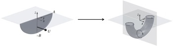
A sketch of the bulk scale effects of deep-water breaking on the water column. We assume that breaking acts like a thin impulsively forced disc of semi-major axis $A$ and semi-minor axis $B$ , being forced from rest to a speed $U$ along the $x$ direction. The disc is then assumed to dissolve, with the flow rolling up where it is strongest, that is along its perimeter, leaving a persistent vortex ring that characterizes the ensemble-averaged post-breaking flow.

Based on these constraints, the authors chose to model $\boldsymbol{{\mathcal{B}}}$ using a thin, impulsively forced half-elliptical disc of semi-major axis $A$ and semi-minor axis $B$ being forced from rest to a speed $U$ along its axis of symmetry, that is in the $x$ -direction, as shown in figure 2. The disc is assumed to dissolve (Taylor Reference Taylor1953), leaving an elliptical vortex ring, whose properties can be easily related to those of the forced disc.

Dhanak & Bernardinis (Reference Dhanak and Bernardinis1981, Appendix A, see also Pizzo & Melville Reference Pizzo and Melville2013) found that the impulse, $I$ , of the elliptical disc can be related to the kinetic energy, $\mathbb{T}$ , of the generated vortex ring by (cf. (2.11)) $I=2\mathbb{T}U^{-1}$ . This is also consistent with the study of Linden & Turner (Reference Linden and Turner2001). We assume this kinetic energy of the disk $\mathbb{T}$ is equivalent to the kinetic energy of the mean flow current ${\mathcal{E}}_{c}$ .

From (2.10), we can relate the impulse in the mean flow currents to the momentum flux lost by the wave field, and associate this with the impulse needed to generate the mean flow vortex. That is, we find

This allows us to rewrite the kinetic energy of the mean flow as

where we have substituted in the formula for the circulation of the elliptical vortex ring found by Dhanak & Bernardinis (Reference Dhanak and Bernardinis1981), i.e.  $\unicode[STIX]{x1D6E4}=2UB$ .

Finally, we define the central focus of our study. Namely, we consider the ratio of the energy in the breaking-induced vortex to the total energy lost due to breaking, which we define as ${\mathcal{R}}_{c}$ , and is given by

where the phase velocity is given by $c=\unicode[STIX]{x1D714}/k=2c_{g}$ for linear deep-water surface gravity waves.

From Rapp & Melville (Reference Rapp and Melville1990, see their figure 34), and the scaling arguments of Pizzo & Melville (Reference Pizzo and Melville2013), the depth to which the fluid is mixed, i.e.  $B$ , scales with $h$ , which together with (1.2) implies that

where $\unicode[STIX]{x1D712}$ is a constant. We will now examine this quantity using direct numerical simulations of breaking waves.

3.1 Numerical experiment

To corroborate our scaling model, we now perform direct numerical simulations (DNS) of the two-dimensional Navier–Stokes equations in a two-phase fluid (air and water) accounting for surface tension and viscous effects using the open source solver Gerris (Popinet Reference Popinet2003, Reference Popinet2009), based on a quad/octree adaptive spatial discretization, multilevel Poisson solver. The interface between the high density liquid (water) and the low density gas (air) is reconstructed by a volume of fluid (VOF) method. This solver has been successfully used in various multiphase problems such as atomization (Fuster et al. Reference Fuster, Agbaglah, Josserand, Popinet and Zaleski2009), the growth of instabilities at the interface (Fuster et al. Reference Fuster, Matas, Marty, Popinet, Hoepffner, Cartellier and Zaleski2013), capillary wave turbulence (Deike et al. Reference Deike, Fuster, Berhanu and Falcon2014) and two- and three-dimensional wave breaking (Fuster et al. Reference Fuster, Agbaglah, Josserand, Popinet and Zaleski2009; Deike et al. Reference Deike, Popinet and Melville2015; Deike, Melville & Popinet Reference Deike, Melville and Popinet2016).

As in Deike et al. (Reference Deike, Popinet and Melville2015, Reference Deike, Melville and Popinet2016), we use nonlinear waves, based on a truncated Stokes expansion, of wavelength $\unicode[STIX]{x1D706}$ , as initial conditions to study wave breaking. Note, this method of generating breaking waves is different from the dispersive focusing technique used in the laboratory. This becomes manifest in the value of the breaking threshold. Indeed, as discussed in Deike et al. (Reference Deike, Popinet and Melville2015, Reference Deike, Melville and Popinet2016), the critical slope for wave breaking changes when a steep Stokes wave is used instead of a dispersive focusing packet or a packet undergoing modulational instability. In the present case, a slope of 0.32 corresponds to an incipient breaking wave, which has total dissipation less than a spilling breaker of the same slope obtained by a dispersive wave focusing technique in the laboratory.

In order to simulate the laboratory experiments, the waves must be able to propagate freely after breaking without interfering with the flow created during the breaking event. Thus we consider a two-dimensional (2-D) rectangular numerical domain, with dimension $L=8\unicode[STIX]{x1D706}$ in the horizontal propagation direction and $l=\unicode[STIX]{x1D706}$ in the vertical direction. The mean water level is set at $\unicode[STIX]{x1D702}=0$ , so that the water depth is $d=\unicode[STIX]{x1D706}/2$ . Boundary conditions are periodic in $x$ , but as we will see the main wave never reaches the end of the numerical domain for times necessary to resolve the properties under investigation. The top and bottom walls are free slip (at $z=\pm d=\unicode[STIX]{x1D706}/2$ ). The total simulation time corresponds to $8T$ , where $T=2\unicode[STIX]{x03C0}/\unicode[STIX]{x1D714}$ is the wave period and $\unicode[STIX]{x1D714}$ the linear angular frequency of the input wave form.

A third-order expansion, based on Stokes waves, is used for the interface $\unicode[STIX]{x1D702}(x,t)$ which together with the velocity potential $\unicode[STIX]{x1D719}(x,z,t)$ in the water constitute the initial conditions at the left of the numerical domain, for $x\in [\unicode[STIX]{x1D706}/2:3\unicode[STIX]{x1D706}/2]$ and in the rest of the domain, the interface and the velocity are set to $0$ by applying a smooth windowing. All cases discussed in this work are single breaking events.

The physical properties of the two phases are those of air and water, and this manifests itself through the density and viscosity ratios. The Bond number is defined as $Bo=\unicode[STIX]{x0394}\unicode[STIX]{x1D70C}g/(\unicode[STIX]{x1D6FE}k^{2})$ , with $\unicode[STIX]{x0394}\unicode[STIX]{x1D70C}$ the density difference between the two fluids, and $\unicode[STIX]{x1D6FE}$ is the surface tension, so that $Bo$ gives the ratio between gravity and surface tension forces. The Reynolds number in the water is $Re=c\unicode[STIX]{x1D706}/\unicode[STIX]{x1D708}$ , where $c=\sqrt{g/k}$ is the linear gravity wave phase speed and $\unicode[STIX]{x1D708}$ is the kinematic viscosity of the water, which is set to $Re=40\,000$ . This choice is related to spatial resolution constraints, but should not affect the results regarding the wave dissipation, since we are at a sufficiently high Reynolds number (Deike et al. Reference Deike, Popinet and Melville2015, Reference Deike, Melville and Popinet2016) to capture the phenomena in question. We choose $Bo=200$ to obtain plunging breakers at high initial wave slope and also to be able to correctly resolve surface tension effects.

We define the characteristic slope to be $S=ak$ , with $a$ the initial wave amplitude and $k=2\unicode[STIX]{x03C0}/\unicode[STIX]{x1D706}$ the wavenumber. $S$ varies from 0.35 to 0.65, i.e. from non-breaking waves to strongly plunging waves (Deike et al. Reference Deike, Popinet and Melville2015). Note slopes higher than the limiting slope for the full Stokes wave solution can be defined as we are generating our conditions based on a third-order Stokes expansion. It is useful to recall that the slope at breaking is proportional to the initial wave slope in this configuration (Deike et al. Reference Deike, Popinet and Melville2015, Reference Deike, Melville and Popinet2016), which is consistent with the laboratory findings of the analogous relationship for focusing packets (Drazen et al. Reference Drazen, Melville and Lenain2008).

Adaptive mesh refinement is used to accurately solve for the interface and the vortex structures, with a mesh size of $\text{d}x=\text{d}y=\unicode[STIX]{x1D706}/512$ , with adaptive criteria on the vorticity and the interface. This configuration allows accurate solutions for the dissipative scales and surface tension effects, as shown by previous two- and three-dimensional simulations (Deike et al. Reference Deike, Popinet and Melville2015, Reference Deike, Melville and Popinet2016). As discussed in Deike et al. (Reference Deike, Popinet and Melville2015, Reference Deike, Melville and Popinet2016), this resolution is enough to have full convergence of the DNS and the results presented here are not sensitive to the mesh size. This is achieved thanks to the adaptive methods on the interface and vorticity, and to our choice of Bond number and Reynolds number. Choosing $Bo=200$ and $Re=40\,000$ permits us to fully resolve the viscous boundary layer and associated dissipative processes, as well as the surface tension effects, without the use of any subgrid model. Moreover, Deike et al. (Reference Deike, Popinet and Melville2015, Reference Deike, Melville and Popinet2016) showed that this value of the Reynolds number is high enough to reproduce the dissipative properties that were observed in the laboratory results; and Deike et al. (Reference Deike, Popinet and Melville2015) showed that the dissipation for breaking waves of slopes $S>0.35$ is not sensitive to the Bond number for $Bo>100$ . This validates our choice of physical parameters and mesh grid size for the present study.

Note, we find that for the breaking waves modelled in this paper, the energy dissipated in the water column dominates (i.e. is more than 96 % of the total energy lost by the wave field, in all tested cases) the energy dissipated in the air. This is consistent with the fact that the density of the water is several orders of magnitude larger than that of the air and agrees with laboratory studies on air flow over breaking waves (Banner & Melville Reference Banner and Melville1976; Veron, Saxena & Misra Reference Veron, Saxena and Misra2007; Belden & Techet Reference Belden and Techet2011).

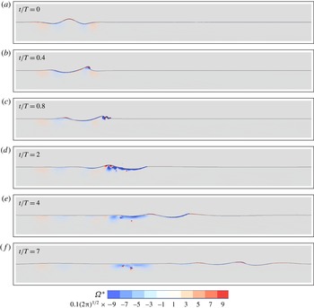
A typical DNS evolution of a breaking wave, with $S=0.55$ , is shown in figure 3. The wave propagates from the left to the right before undergoing strongly nonlinear behaviour leading to breaking. A jet is formed at the front of the wave that subsequently impacts the water surface. The time of the breaking event, or impact with the surface, $t_{b}$ , occurs between $t/T=0.5$ and $t/T=1$ , as in Deike et al. (Reference Deike, Popinet and Melville2015, Reference Deike, Melville and Popinet2016), while the jet impacts the free surface at approximately $x_{b}=x/\unicode[STIX]{x1D706}\approx 2.5$ . Figure 3 shows that the breaking event generates turbulent motion and strong vortical structures in the water in the area bounded by $x\in [2.5:3.5]\unicode[STIX]{x1D706}$ . This defines the breaking area. After breaking, the waves are transmitted and radiated from the breaking region, subsequently rendering the free surface as a rigid lid in this area, which is consistent with the laboratory studies and figure 1. However, the breaking-induced current, characterized by the vortex, is still present in the breaking region several periods after $t_{b}$ .

Figure 3.

Time evolution of a plunging breaker with the vorticity field $\unicode[STIX]{x1D6FA}^{\ast }=\unicode[STIX]{x1D6FA}/\unicode[STIX]{x1D714}$ at different time steps. The wave starts at the left of the numerical domain, propagates to the right and breaks after half a period of propagation. The waves then propagate out of the region where breaking occurred, leaving an active vorticity field that characterizes the post-breaking flow. The initial conditions were chosen such that $S=0.55$ , $Re=4\times 10^{4}$ , $Bo=200$ .

Figure 4.

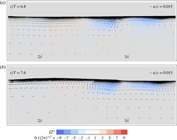
The normalized vorticity field $\unicode[STIX]{x1D6FA}^{\ast }$ remaining in the region after a plunging breaker, and after the remaining waves have propagated away. The post-breaking flow is characterized by a compact region of vorticity, outside of which the flow is largely irrotational. $Re=4\times 10^{4}$ , $Bo=200$ and $S=0.5$ .

Here, we focus on post-breaking flow properties and the resulting vorticity, and its associated circulation, as well as the kinetic energy flux of the current in the breaking area, for long times after the waves have propagated away.

As was discussed above, the generated vortical structure has been observed experimentally and was found to be a coherent vortex by Rapp & Melville (Reference Rapp and Melville1990), Melville et al. (Reference Melville, Veron and White2002), which was described in more detail by Pizzo & Melville (Reference Pizzo and Melville2013). Figure 4 shows a close up of this area several periods after breaking. A coherent vortex is indeed observed and remains stable, slowly moving towards the right of the numerical domain. Its intensity slowly decreases due to viscous dissipation, consistent with Melville et al. (Reference Melville, Veron and White2002). Recall, $\unicode[STIX]{x1D6FA}^{\ast }$ is the vorticity field normalized by the characteristic angular frequency $\unicode[STIX]{x1D714}$ , in the $y$ direction.

3.2 Energy dissipated by breaking, circulation and mean currents

We now calculate the integral properties of the breaking waves for various slopes $S$ . To begin, we compute the energy flux ${\mathcal{F}}$ , i.e. equation (2.5), by relating this to the energy density, $E$ , through linear theory (far upstream and downstream of the breaking event), where

That is, the energy flux at a given location is then ${\mathcal{F}}(x)=c_{g}E(x)$ where $c_{g}=(1/2)c$ is the group velocity of the wave and $c$ is the phase speed. As defined in § 2, the change in energy flux due to breaking is then given by $\unicode[STIX]{x0394}{\mathcal{F}}=c_{g}\unicode[STIX]{x0394}E$ . Note, following the laboratory experiments of Drazen et al. (Reference Drazen, Melville and Lenain2008), this relation assumes that the group velocity is approximately equal before and after breaking (see also Pizzo & Melville Reference Pizzo and Melville2016). The dissipated energy flux per unit length of breaking crest $\unicode[STIX]{x1D716}_{l}$ is then given by $\unicode[STIX]{x1D716}_{l}=|\unicode[STIX]{x0394}{\mathcal{F}}|/\unicode[STIX]{x1D70F}_{b}$ , where $\unicode[STIX]{x1D70F}_{b}$ is the active breaking time and in these experiments it is found that $\unicode[STIX]{x1D70F}_{b}\approx T$ which is consistent with other laboratory (Drazen et al. Reference Drazen, Melville and Lenain2008) and numerical studies (Deike et al. Reference Deike, Popinet and Melville2015, Reference Deike, Melville and Popinet2016).

Figure 5.

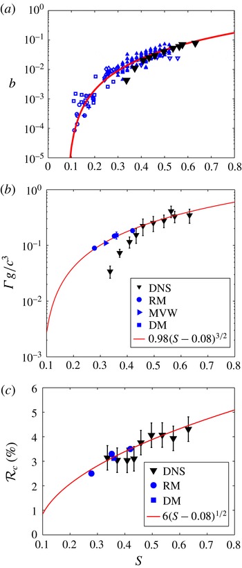
In all three plots, (▾) are DNS data. (a) Breaking parameter $b$ as a function of the initial wave slope $S$ . Solid line: semi-empirical formulation based on scaling argument, $b=0.4(S-0.08)^{5/2}$ (Romero et al. Reference Romero, Melville and Kleiss2012). Blue symbols are experimental data; triangles and diamonds are from Drazen et al. (Reference Drazen, Melville and Lenain2008), cross and circle are from Banner & Peirson (Reference Banner and Peirson2007) and squares are from Grare et al. (Reference Grare, Peirson, Branger, Walker, Giovanangeli and Makin2013). The differences between experiments and DNS at lower values of $S$ come from differences in initiating wave breaking. (b) Circulation generated by the breaking event $\unicode[STIX]{x1D6E4}$ (normalized by $c^{3}/g$ ) as a function of $S$ . Solid line is the model from Pizzo & Melville (Reference Pizzo and Melville2013) fitted to experimental data, $\unicode[STIX]{x1D6E4}g/c^{3}=\unicode[STIX]{x1D6FE}_{0}(S-S_{0})^{3/2}$ , where $\unicode[STIX]{x1D6FE}_{0}=0.98$ and $S_{0}=0.08$ . Blue closed circles are from Rapp & Melville (Reference Rapp and Melville1990), the right triangle is from Melville et al. (Reference Melville, Veron and White2002) and the square is from Drazen & Melville (Reference Drazen and Melville2009). (c) Ratio of the energy flux in the current (created by the breaking event) and the dissipated energy flux due to the breaking wave, ${\mathcal{R}}_{c}$ . Blue closed circles (RM): laboratory data from Rapp & Melville (Reference Rapp and Melville1990); closed blue square (DM) is a data point from Drazen & Melville (Reference Drazen and Melville2009). Solid line is ${\mathcal{R}}_{c}={\mathcal{E}}_{c}/|\unicode[STIX]{x0394}F|=\unicode[STIX]{x1D712}(S-S_{0})^{1/2}$ based on the model presented in § 2, equation (2.18) and including an empirical threshold slope, equation (3.2), with $S_{0}=0.08$ and $\unicode[STIX]{x1D712}=0.06$ the best fit to the data.

Figure 5(a) shows the breaking parameter $b$ as a function of the slope $S$ in the DNS and in available laboratory data. The breaking parameter $b$ as a function of the slope $S$ in the present DNS is found in good agreement with previous experimental results and the semi-empirical model of Drazen et al. (Reference Drazen, Melville and Lenain2008, see also Grare et al. (Reference Grare, Peirson, Branger, Walker, Giovanangeli and Makin2013)) and Romero et al. (Reference Romero, Melville and Kleiss2012) for strong breaking waves, as in our previous numerical work (Deike et al. Reference Deike, Popinet and Melville2015, Reference Deike, Melville and Popinet2016). The difference in the dissipation between experiments and DNS for $S$ between 0.35 and 0.4 is most likely related to the route to breaking, i.e. how the initial conditions are chosen. Indeed, as discussed in Deike et al. (Reference Deike, Popinet and Melville2015, Reference Deike, Melville and Popinet2016), the critical slope for wave breaking changes when a steep Stokes wave is used instead of a dispersive focusing packet or a packet undergoing modulational instability. In the present case, a slope of 0.32 corresponds to an incipient breaking wave, which has total dissipation less than a spilling breaker of the same slope obtained by a dispersive wave focusing technique in the laboratory. Note, other numerical studies have examined the dissipation due to breaking waves and have found results compatible with the one presented here and in Deike et al. (Reference Deike, Popinet and Melville2015, Reference Deike, Melville and Popinet2016) (see the two-dimensional DNS of Iafrati Reference Iafrati2011), and the two- and three-dimensional large eddy simulation (LES) of Derakhti & Kirby (Reference Derakhti and Kirby2014), Lubin & Glockner (Reference Lubin and Glockner2015), and Derakhti & Kirby (Reference Derakhti and Kirby2016).

The integrated vorticity and the kinetic energy flux over the breaking area are approximately constant with time, slowly decreasing due to viscous dissipative effects, which is consistent with the laboratory studies of Melville et al. (Reference Melville, Veron and White2002). The circulation $\unicode[STIX]{x1D6E4}$ given by (2.14), is averaged over two wave periods, starting four wave periods after the breaking event when the waves have propagated out of the region of breaking. The error bars on $\unicode[STIX]{x1D6E4}$ in the DNS are representative of its sensitivity to the area and time of integration.

Figure 5(b) shows $\unicode[STIX]{x1D6E4}$ as a function of the wave slope, compared to the limited available laboratory data and the corresponding scaling from Pizzo & Melville (Reference Pizzo and Melville2013) for the circulation, $\unicode[STIX]{x1D6E4}=\unicode[STIX]{x1D6FE}_{0}(S-S_{0})^{3/2}$ , where $\unicode[STIX]{x1D6FE}_{0}$ is an order-one constant and $S_{0}$ is the threshold for breaking. The experimental data presented in figure 5(b) are from the laboratory studies of Rapp (Reference Rapp1986), Rapp & Melville (Reference Rapp and Melville1990), Melville et al. (Reference Melville, Veron and White2002), Drazen & Melville (Reference Drazen and Melville2009), who computed either explicitly the circulation or provided the measurements of the velocity fields. This is discussed in detail in Pizzo & Melville (Reference Pizzo and Melville2013). The constant $\unicode[STIX]{x1D6FE}_{0}=0.98$ was found by a best fit with the data presented in Pizzo & Melville (Reference Pizzo and Melville2013) and shown by the blue circles in 5(b), while $S_{0}=0.08$ is the threshold that best fits multiple laboratory studies, as discussed in Romero et al. (Reference Romero, Melville and Kleiss2012). Good agreement is found between the model for $\unicode[STIX]{x1D6E4}$ and the available experimental data and the numerical results for large values of $S$ . This is consistent with the findings of Deike et al. (Reference Deike, Popinet and Melville2015, Reference Deike, Melville and Popinet2016) for the energy dissipation rate, where as mentioned above it is noticed that the different breaking generation methods between the laboratory and the numerical experiments are manifest in the breaking threshold parameter $S_{0}$ .

Finally, figure 5(c) shows the main result of this paper, namely the ratio of the energy flux transferred to the current to the dissipated energy flux due to the breaking wave, i.e.  ${\mathcal{R}}_{c}$ . Note, following the laboratory studies of (Melville et al. Reference Melville, Veron and White2002), and consistent with the theoretical assumptions made in § 2, we have assumed that the energy remaining in the region of breaking is entirely in the mean flow. Figure 5(c) shows ${\mathcal{R}}_{c}$ as a function of the wave slope in the present DNS, together with the experimental data from Rapp & Melville (Reference Rapp and Melville1990), Drazen & Melville (Reference Drazen and Melville2009) (note that Melville et al. (Reference Melville, Veron and White2002) provided a measure of $\unicode[STIX]{x1D6E4}$ ; however, they did not provide a measure of ${\mathcal{E}}_{c}$ ). The data are well described by the scaling given by (2.18), including the breaking threshold,

with $\unicode[STIX]{x1D712}=0.06$ and $S_{0}=0.08$ is the critical slope determined by Romero et al. (Reference Romero, Melville and Kleiss2012). The value $\unicode[STIX]{x1D712}=0.06$ is the least-squares fit to the laboratory and numerical data. Note that there is a physical relation between $\unicode[STIX]{x1D6E4}$ and ${\mathcal{E}}_{c}$ , and dimensionally we get ${\mathcal{E}}_{c}\propto \unicode[STIX]{x1D70C}\unicode[STIX]{x1D6E4}^{2}$ . This allows us to perform a consistency check on our relationship given in (2.18). Namely, we have ensured that values of $b$ , consistent with the laboratory and numerical data, can be retrieved from $\unicode[STIX]{x1D6E4}$ and ${\mathcal{R}}_{c}$ , where ${\mathcal{R}}_{c}\propto (\unicode[STIX]{x1D6E4}g/c^{3})^{2}/b$ .

We find that ${\mathcal{R}}_{c}$ varies from 2 % to 5 % for slopes corresponding to incipient breaking waves to strong plunging events, in good agreement with the earlier experimental results from Rapp & Melville (Reference Rapp and Melville1990) as well as an additional point from the laboratory data of Drazen & Melville (Reference Drazen and Melville2009). Note, the number of these measurements that is available is limited, as one must measure the kinetic energy in the region of breaking several wave periods after the breaking event. This is why there are far fewer measurements of this quantity versus, for example, the energy dissipation rate per unit length of breaking crest $\unicode[STIX]{x1D716}_{l}$ . The scatter in the numerical data comes from the difficulties in properly estimating a small difference between two large quantities (energy flux before and after breaking) and the fact that the ratio ${\mathcal{R}}_{c}$ is a small quantity. Finally the agreement with the scaling argument presented in § 2 is encouraging. In the next section, we discuss some of the implications of these results.