2.1 Critical wavenumber

It is known that the class-III resonance occurs only when the slope of the dispersion curve for the surface wave at $(k_{1},\unicode[STIX]{x1D714}_{1})$ is smaller than that for the internal wave at $(K,\unicode[STIX]{x1D6FA})=(0,0)$ (see figure 1a). This can happen only when $k_{1}$ is greater than a certain critical value $k_{c}$. Considering that the two dispersion curves should be tangent to each other as $k_{1}(=k_{2})\rightarrow k_{c}$ and $K\rightarrow 0$, the critical surface wavenumber can be found by matching the slopes of the two curves: $\text{d}\unicode[STIX]{x1D6FA}/\text{d}K|_{K=0}=\text{d}\unicode[STIX]{x1D714}/\text{d}k|_{k=k_{c}}$. From $\text{d}\unicode[STIX]{x1D6FA}/\text{d}K|_{K=0}=\unicode[STIX]{x1D6FA}/K|_{K=0}$, the criticality condition implies that the linear long wave speed of the internal wave $C_{0}=\unicode[STIX]{x1D6FA}/K|_{K=0}$ and the group velocity of the surface wave $c_{g}(k_{c})=\text{d}\unicode[STIX]{x1D714}/\text{d}k|_{k=k_{c}}$ must be equal to each other so that

(2.3)$$\begin{eqnarray}C_{0}=c_{g}(k_{c}),\end{eqnarray}$$

where $C_{0}$ is the linear long internal wave speed given by

(2.4)$$\begin{eqnarray}{C_{0}}^{2}=\frac{gh_{1}h_{2}(\unicode[STIX]{x1D70C}_{2}-\unicode[STIX]{x1D70C}_{1})}{\unicode[STIX]{x1D70C}_{1}h_{2}+\unicode[STIX]{x1D70C}_{2}h_{1}}.\end{eqnarray}$$

Then, it can be concluded from (2.3) that the class-III resonance is always possible when at least one of the surface wavenumbers is greater than $k_{c}$, which depends on the density and depth ratios: $k_{c}=k_{c}(\unicode[STIX]{x1D70C}_{1}/\unicode[STIX]{x1D70C}_{2},h_{1}/h_{2})$.

Figure 2.

The critical wavenumber $k_{c}h_{1}$ as a function of the density ratio for $\unicode[STIX]{x1D70C}_{1}/\unicode[STIX]{x1D70C}_{2}$ between 0.85 and 1 for three different depth ratios: $h_{1}/h_{2}=10$ (solid); $h_{1}/h_{2}=1$ (dashed); $h_{1}/h_{2}=1/2$ (dotted).

Figure 2 shows the dimensionless critical wavenumber $k_{c}h_{1}$ as a function of density ratio $\unicode[STIX]{x1D70C}_{1}/\unicode[STIX]{x1D70C}_{2}$ for values of the latter between 0.85 and 1 for different depth ratios $h_{1}/h_{2}$. The critical wavenumber $k_{c}h_{1}$ increases with $\unicode[STIX]{x1D70C}_{1}/\unicode[STIX]{x1D70C}_{2}$ and $h_{1}/h_{2}$. As the density ratio $\unicode[STIX]{x1D70C}_{1}/\unicode[STIX]{x1D70C}_{2}\rightarrow 1$, the dimensionless critical wavenumber $k_{c}h_{1}$ increases rapidly and, therefore, only short surface waves satisfy the class-III resonance conditions given by (2.2). For example, for $\unicode[STIX]{x1D70C}_{1}/\unicode[STIX]{x1D70C}_{2}=0.99$ and $h_{1}/h_{2}=1/2$, one can find $k_{c}h_{1}\simeq 37.42$ so that the critical wavelength $\unicode[STIX]{x1D706}_{c}=2\unicode[STIX]{x03C0}/k_{c}$ is given by $\unicode[STIX]{x1D706}_{c}/h_{1}\simeq 0.168$.

2.2 Group resonance condition near criticality

Near criticality, the two surface wavenumbers $k_{1}$ and $k_{2}$ are close to each other so that $k_{2}$ can be written as $k_{2}=k_{1}(1\pm K/k_{1})$ with $K/k_{1}\ll 1$. When $\unicode[STIX]{x1D714}_{2}=\unicode[STIX]{x1D714}(k_{2})$ is expanded around $k_{1}$, one can show that

(2.5)$$\begin{eqnarray}\unicode[STIX]{x1D714}_{1}-\unicode[STIX]{x1D714}_{2}\pm \unicode[STIX]{x1D6FA}=\mp \frac{\text{d}\unicode[STIX]{x1D714}}{\text{d}k}\bigg|_{k_{1}}K\pm \unicode[STIX]{x1D6FA}+O(K/k_{1})^{2}.\end{eqnarray}$$

This implies that the resonance condition given by (2.2b) can be satisfied approximately under the so-called group resonance condition defined by

(2.6)$$\begin{eqnarray}C|_{K}\simeq c_{g}|_{k_{g}},\end{eqnarray}$$

where $k_{g}$ is the wavenumber of the carrier wave whose group velocity matches the phase speed of the internal wave $C=\unicode[STIX]{x1D6FA}/K$. This condition is a slight modification to (2.3) for an internal wave whose wavenumber is small, but not zero.

Since (2.6) is an approximation to (2.2b), its solution $k_{g}$ is slightly different from $k_{1\pm }$, which are the solutions of the exact resonance condition (2.2) for a fixed value of $K$. Therefore, the triads of $(k_{g},k_{g}\pm K,K)$ satisfy a near-resonance condition.

In this paper, we develop an explicit Hamiltonian system and study the near-resonant triad interactions between short surface and long internal waves under the group resonance condition. Then the results will be compared with previous theoretical and experimental results.

3.1 Basic equations

We consider a system of two layers with constant densities, where the $i$th layer ($i=1,2$) is bounded by the upper and lower boundaries located at $z=\unicode[STIX]{x1D702}_{i}(\boldsymbol{x},t)$ and $z=\unicode[STIX]{x1D702}_{i+1}(\boldsymbol{x},t)$, respectively, with $\boldsymbol{x}=(x,y)$. Here, $\unicode[STIX]{x1D702}_{1}=\unicode[STIX]{x1D701}_{1}$, $\unicode[STIX]{x1D702}_{2}=-h_{1}+\unicode[STIX]{x1D701}_{2}$, $\unicode[STIX]{x1D702}_{3}=-(h_{1}+h_{2})$ with $\unicode[STIX]{x1D701}_{1}(\boldsymbol{x},t)$ and $\unicode[STIX]{x1D701}_{2}(\boldsymbol{x},t)$ being the surface and interface displacements, respectively (see figure 3).

Under the potential flow assumption, the kinematic boundary condition at the upper boundary of the $i$th layer is given, after using the chain rule, by

(3.1)$$\begin{eqnarray}\frac{\unicode[STIX]{x2202}\unicode[STIX]{x1D701}_{i}}{\unicode[STIX]{x2202}t}+\unicode[STIX]{x1D735}\unicode[STIX]{x1D6F7}_{i}\boldsymbol{\cdot }\unicode[STIX]{x1D735}\unicode[STIX]{x1D701}_{i}=\left(1+|\unicode[STIX]{x1D735}\unicode[STIX]{x1D701}_{i}|^{2}\right)W_{i},\end{eqnarray}$$

where $\unicode[STIX]{x1D735}$ is the horizontal gradient, and $i=1$ and 2 correspond to the upper and lower layers, respectively. Here, $\unicode[STIX]{x1D6F7}_{i}$ and $W_{i}$ are the velocity potential and the vertical velocity, respectively, evaluated at $z=\unicode[STIX]{x1D702}_{i}$ such that $\unicode[STIX]{x1D6F7}_{i}(\boldsymbol{x},t)\equiv \unicode[STIX]{x1D719}_{i}(\boldsymbol{x},z=\unicode[STIX]{x1D702}_{i},t)$ and $W_{i}(\boldsymbol{x},t)\equiv \unicode[STIX]{x2202}\unicode[STIX]{x1D719}_{i}/\unicode[STIX]{x2202}z(\boldsymbol{x},z=\unicode[STIX]{x1D702}_{i},t)$, with $\unicode[STIX]{x1D719}_{i}$ being the solution of the three-dimensional Laplace equation for the $i$th layer. In addition, the kinematic boundary condition at the interface ($z=\unicode[STIX]{x1D702}_{2}$) can be written, in terms of the velocity potential for the upper layer, as

(3.2)$$\begin{eqnarray}\frac{\unicode[STIX]{x2202}\unicode[STIX]{x1D701}_{2}}{\unicode[STIX]{x2202}t}+\unicode[STIX]{x1D735}\unicode[STIX]{x1D6F7}_{1}^{\ast }\boldsymbol{\cdot }\unicode[STIX]{x1D735}\unicode[STIX]{x1D701}_{2}=\left(1+|\unicode[STIX]{x1D735}\unicode[STIX]{x1D701}_{2}|^{2}\right)W_{1}^{\ast }.\end{eqnarray}$$

Here, the variables with asterisks represent those evaluated at the interface such that $\unicode[STIX]{x1D6F7}_{1}^{\ast }\equiv \unicode[STIX]{x1D719}_{1}|_{z=\unicode[STIX]{x1D702}_{2}}$ and $W_{1}^{\ast }\equiv \unicode[STIX]{x2202}\unicode[STIX]{x1D719}_{1}/\unicode[STIX]{x2202}z|_{z=\unicode[STIX]{x1D702}_{2}}$. When combined with (3.1), the second kinematic condition given by (3.2) can be written as

(3.3)$$\begin{eqnarray}W_{1}^{\ast }-\frac{\unicode[STIX]{x1D735}\unicode[STIX]{x1D701}_{2}}{1+|\unicode[STIX]{x1D735}\unicode[STIX]{x1D701}_{2}|^{2}}\boldsymbol{\cdot }\unicode[STIX]{x1D735}\unicode[STIX]{x1D6F7}_{1}^{\ast }=W_{2}-\frac{\unicode[STIX]{x1D735}\unicode[STIX]{x1D701}_{2}}{1+|\unicode[STIX]{x1D735}\unicode[STIX]{x1D701}_{2}|^{2}}\boldsymbol{\cdot }\unicode[STIX]{x1D735}\unicode[STIX]{x1D6F7}_{2},\end{eqnarray}$$

which implies continuity of the normal velocities at the interface located at $z=\unicode[STIX]{x1D702}_{2}$, or $z=-h_{2}+\unicode[STIX]{x1D701}_{2}(x,t)$.

On the other hand, the dynamic boundary conditions at the top free surface and interface are given by

(3.4a,b)$$\begin{eqnarray}P_{1}=P_{atm}\quad \text{at }z=\unicode[STIX]{x1D702}_{1},\quad P_{2}=P_{1}^{\ast }\quad \text{at }z=\unicode[STIX]{x1D702}_{2},\end{eqnarray}$$

where $P_{i}$ ($i=1,2$) are the pressures evaluated at $z=\unicode[STIX]{x1D702}_{i}$ while $P_{1}^{\ast }$ is the pressure of the upper layer evaluated at the interface $(z=\unicode[STIX]{x1D702}_{2})$. Here, $P_{atm}$ is the applied atmospheric pressure in the presence of wind; otherwise, $P_{atm}=0$. From the Bernoulli equation given, after being evaluated at $z=\unicode[STIX]{x1D702}_{i}$, by

(3.5)$$\begin{eqnarray}\frac{\unicode[STIX]{x2202}\unicode[STIX]{x1D6F7}_{i}}{\unicode[STIX]{x2202}t}+g\unicode[STIX]{x1D702}_{i}+\frac{1}{2}|\unicode[STIX]{x1D735}\unicode[STIX]{x1D6F7}_{i}|^{2}+\frac{P_{i}}{\unicode[STIX]{x1D70C}_{i}}=\frac{1}{2}(1+|\unicode[STIX]{x1D735}\unicode[STIX]{x1D701}_{i}|^{2}){W_{i}}^{2},\end{eqnarray}$$

the dynamic boundary conditions (3.4) can be written as

(3.6)$$\begin{eqnarray}\displaystyle & \displaystyle \frac{\unicode[STIX]{x2202}\unicode[STIX]{x1D6F9}_{1}}{\unicode[STIX]{x2202}t}=-\unicode[STIX]{x1D70C}_{1}g\unicode[STIX]{x1D701}_{1}-\frac{1}{2}\unicode[STIX]{x1D70C}_{1}|\unicode[STIX]{x1D735}\unicode[STIX]{x1D6F7}_{1}|^{2}+\frac{1}{2}\unicode[STIX]{x1D70C}_{1}(1+|\unicode[STIX]{x1D735}\unicode[STIX]{x1D701}_{1}|^{2}){W_{1}}^{2}-P_{atm}, & \displaystyle\end{eqnarray}$$

(3.7)$$\begin{eqnarray}\displaystyle & \displaystyle \frac{\unicode[STIX]{x2202}\unicode[STIX]{x1D6F9}_{2}}{\unicode[STIX]{x2202}t}=-\unicode[STIX]{x0394}\unicode[STIX]{x1D70C}g\unicode[STIX]{x1D701}_{2}-\frac{1}{2}(\unicode[STIX]{x1D70C}_{2}|\unicode[STIX]{x1D735}\unicode[STIX]{x1D6F7}_{2}|^{2}-\unicode[STIX]{x1D70C}_{1}|\unicode[STIX]{x1D735}\unicode[STIX]{x1D6F7}_{1}^{\ast }|^{2})+\frac{1}{2}(1+|\unicode[STIX]{x1D735}\unicode[STIX]{x1D701}_{2}|^{2})(\unicode[STIX]{x1D70C}_{2}{W_{2}}^{2}-\unicode[STIX]{x1D70C}_{1}{W_{1}^{\ast }}^{2}),\quad & \displaystyle\end{eqnarray}$$

where $\unicode[STIX]{x0394}\unicode[STIX]{x1D70C}=\unicode[STIX]{x1D70C}_{2}-\unicode[STIX]{x1D70C}_{1}>0$ for stable stratification and $\unicode[STIX]{x1D6F9}_{i}$ are defined as

(3.8a,b)$$\begin{eqnarray}\unicode[STIX]{x1D6F9}_{1}=\unicode[STIX]{x1D70C}_{1}\unicode[STIX]{x1D6F7}_{1},\quad \unicode[STIX]{x1D6F9}_{2}=\unicode[STIX]{x1D70C}_{2}\unicode[STIX]{x1D6F7}_{2}-\unicode[STIX]{x1D70C}_{1}\unicode[STIX]{x1D6F7}_{1}^{\ast }.\end{eqnarray}$$

Once $\unicode[STIX]{x1D6F7}_{i}$, $W_{i}$, $\unicode[STIX]{x1D6F7}_{1}^{\ast }$ and $W_{1}^{\ast }$ can be expressed in terms of $\unicode[STIX]{x1D701}_{i}$ and $\unicode[STIX]{x1D6F9}_{i}$, equations (3.1) and (3.6)–(3.7) yield a closed system of nonlinear evolution equations for $\unicode[STIX]{x1D701}_{i}$ and $\unicode[STIX]{x1D6F9}_{i}$ ($i=1,2$).

As shown by Benjamin & Bridges (Reference Benjamin and Bridges1997) for unbounded two-layer flows, the system for $\unicode[STIX]{x1D701}_{i}$ and $\unicode[STIX]{x1D6F9}_{i}$ is of particular interest as it is known to have a Hamiltonian structure such that

(3.9a,b)$$\begin{eqnarray}\frac{\unicode[STIX]{x2202}\unicode[STIX]{x1D701}_{i}}{\unicode[STIX]{x2202}t}=\frac{\unicode[STIX]{x1D6FF}E}{\unicode[STIX]{x1D6FF}\unicode[STIX]{x1D6F9}_{i}},\quad \frac{\unicode[STIX]{x2202}\unicode[STIX]{x1D6F9}_{i}}{\unicode[STIX]{x2202}t}=-\frac{\unicode[STIX]{x1D6FF}E}{\unicode[STIX]{x1D6FF}\unicode[STIX]{x1D701}_{i}},\end{eqnarray}$$

where $E=E_{p}+E_{K}$ is the total energy with the potential energy $E_{p}$ and the kinetic energy $E_{K}$ given by

(3.10)$$\begin{eqnarray}\displaystyle & \displaystyle E_{P}=\frac{1}{2}\int \left[\unicode[STIX]{x1D70C}_{1}g{\unicode[STIX]{x1D701}_{1}}^{2}+(\unicode[STIX]{x1D70C}_{2}-\unicode[STIX]{x1D70C}_{1})g{\unicode[STIX]{x1D701}_{1}}^{2}\right]\,\text{d}\boldsymbol{x}, & \displaystyle\end{eqnarray}$$

(3.11)$$\begin{eqnarray}\displaystyle & \displaystyle E_{K}=\frac{1}{2}\int \left(\mathop{\sum }_{i=1}^{2}\unicode[STIX]{x1D6F9}_{i}\frac{\unicode[STIX]{x2202}\unicode[STIX]{x1D701}_{i}}{\unicode[STIX]{x2202}t}\right)\,\text{d}\boldsymbol{x}. & \displaystyle\end{eqnarray}$$

For weakly nonlinear waves with $\unicode[STIX]{x1D716}\ll 1$ being the typical wave steepness, the nonlinear evolution equations given by (3.1) and (3.6)–(3.7) can be truncated at $O(\unicode[STIX]{x1D716}^{2})$ as

(3.12a,b)$$\begin{eqnarray}\displaystyle \frac{\unicode[STIX]{x2202}\unicode[STIX]{x1D701}_{1}}{\unicode[STIX]{x2202}t}=W_{1}-\unicode[STIX]{x1D735}\unicode[STIX]{x1D6F7}_{1}\boldsymbol{\cdot }\unicode[STIX]{x1D735}\unicode[STIX]{x1D701}_{1}+O(\unicode[STIX]{x1D716}^{3}),\quad \frac{\unicode[STIX]{x2202}\unicode[STIX]{x1D701}_{2}}{\unicode[STIX]{x2202}t}=W_{2}-\unicode[STIX]{x1D735}\unicode[STIX]{x1D6F7}_{2}\boldsymbol{\cdot }\unicode[STIX]{x1D735}\unicode[STIX]{x1D701}_{2}+O(\unicode[STIX]{x1D716}^{3}),\end{eqnarray}$$

(3.13)$$\begin{eqnarray}\displaystyle & \displaystyle \frac{\unicode[STIX]{x2202}\unicode[STIX]{x1D6F9}_{1}}{\unicode[STIX]{x2202}t}=-\unicode[STIX]{x1D70C}_{1}g\unicode[STIX]{x1D701}_{1}-\frac{1}{2}|\unicode[STIX]{x1D735}\unicode[STIX]{x1D6F9}_{1}|^{2}/\unicode[STIX]{x1D70C}_{1}+\frac{1}{2}\unicode[STIX]{x1D70C}_{1}{W_{1}}^{2}+O(\unicode[STIX]{x1D716}^{3}), & \displaystyle\end{eqnarray}$$

(3.14)$$\begin{eqnarray}\displaystyle & \displaystyle \frac{\unicode[STIX]{x2202}\unicode[STIX]{x1D6F9}_{2}}{\unicode[STIX]{x2202}t}=-\unicode[STIX]{x0394}\unicode[STIX]{x1D70C}g\unicode[STIX]{x1D701}_{2}-\frac{1}{2}\left(\unicode[STIX]{x1D70C}_{2}|\unicode[STIX]{x1D735}\unicode[STIX]{x1D6F7}_{2}|^{2}-\unicode[STIX]{x1D70C}_{1}|\unicode[STIX]{x1D735}\unicode[STIX]{x1D6F7}_{1}^{\ast }|^{2}\right)+\frac{1}{2}\left(\unicode[STIX]{x1D70C}_{2}{W_{2}}^{2}-\unicode[STIX]{x1D70C}_{1}{W_{1}^{\ast }}^{2}\right)+O(\unicode[STIX]{x1D716}^{3}),\quad & \displaystyle\end{eqnarray}$$

where $W_{i}=O(|\unicode[STIX]{x1D735}\unicode[STIX]{x1D701}_{i}|)=O(|\unicode[STIX]{x1D735}\unicode[STIX]{x1D6F7}_{i}|)=O(|\unicode[STIX]{x1D735}\unicode[STIX]{x1D6F9}_{i}|)=O(\unicode[STIX]{x1D716})$ have been assumed on the right-hand sides.

In the followings, using asymptotic expansion correct up to $O(\unicode[STIX]{x1D716}^{2})$, we first find the explicit expressions for $W_{i}$ ($i=1,2$) correct to $O(\unicode[STIX]{x1D716}^{2})$ and those for $W_{1}^{\ast }$, and $\unicode[STIX]{x1D6F7}_{1}^{\ast }$ correct to $O(\unicode[STIX]{x1D716})$ in terms of $\unicode[STIX]{x1D701}_{i}$ and $\unicode[STIX]{x1D6F7}_{i}$. Then, by expressing $\unicode[STIX]{x1D6F7}_{i}$ in terms of $\unicode[STIX]{x1D701}_{i}$ and $\unicode[STIX]{x1D6F9}_{i}$, we obtain a closed system for $\unicode[STIX]{x1D701}_{i}$ and $\unicode[STIX]{x1D6F9}_{i}$.

3.2 Linear solutions

The solution of the Laplace equation for the $i$th layer can be written as

(3.15)$$\begin{eqnarray}\displaystyle \unicode[STIX]{x1D719}_{i}(\boldsymbol{k},z,t)=A_{i}(\boldsymbol{k},t)\cosh (kz)+B_{i}(\boldsymbol{k},t)\sinh (kz). & & \displaystyle\end{eqnarray}$$

To determine $A_{i}$ and $B_{i}$, we impose the following linearized boundary conditions at $z=z_{i}$ and $z=z_{i+1}$ for $i=1,2$

(3.16)$$\begin{eqnarray}\displaystyle & \displaystyle \unicode[STIX]{x1D719}_{i}=\overline{\unicode[STIX]{x1D719}}_{i}\quad \text{at }z=z_{i}, & \displaystyle\end{eqnarray}$$

(3.17)$$\begin{eqnarray}\displaystyle & \displaystyle \frac{\unicode[STIX]{x2202}\unicode[STIX]{x1D719}_{i}}{\unicode[STIX]{x2202}z}=w_{i}^{\ast }\quad \text{at }z=z_{i+1}, & \displaystyle\end{eqnarray}$$

where $z=z_{i}$ and $z=z_{i+1}$ are the mean positions of the upper and lower boundaries, respectively, of the $i$th layer so that $z_{1}=0$, $z_{2}=-h_{1}$ and $z_{3}=-(h_{1}+h_{2})$. Here, we impose the Dirichlet and Neumann boundary conditions at the mean upper and lower boundaries, respectively, for convenience in the derivation of a model. For example, for the lower layer ($i=2$), the zero Neumann condition ($w_{2}^{\ast }=0$) needs to be imposed at $z=z_{3}$ as the vertical velocity vanishes at the bottom. After imposing the boundary conditions given by (3.16) and (3.17) on the solution of the Laplace equation given by (3.15), we attempt to find the expressions for $\overline{w}_{i}$ and $\unicode[STIX]{x1D719}_{i}^{\ast }$ in terms of $\overline{\unicode[STIX]{x1D719}}_{i}$ and $w_{i}^{\ast }$. Notice that $\overline{f}_{i}$ and $f_{i}^{\ast }$ represent the variables evaluated at $z=z_{i}$ and $z=z_{i+1}$, respectively.

The linear solution for the $i$th layer satisfying the boundary conditions given by (3.16)–(3.17) can be found as

(3.18)$$\begin{eqnarray}\unicode[STIX]{x1D719}_{i}=\frac{1}{k\cosh [k(z_{i}-z_{i+1})]}(k\cosh [k(z-z_{i+1})]\overline{\unicode[STIX]{x1D719}}_{i}+\sinh [k(z-z_{i})]w_{i}^{\ast }).\end{eqnarray}$$

Then, the expressions for $\overline{w}_{i}=\unicode[STIX]{x2202}\unicode[STIX]{x1D719}_{i}/\unicode[STIX]{x2202}z|_{z=z_{i}}$ and $\unicode[STIX]{x1D719}_{i}^{\ast }=\unicode[STIX]{x1D719}_{i}|_{z=z_{i+1}}$ can be obtained, in terms of $\overline{\unicode[STIX]{x1D719}}_{i}$ and $w_{i}^{\ast }$, as

(3.19a,b)$$\begin{eqnarray}\overline{w}_{i}=kT_{i}\overline{\unicode[STIX]{x1D719}}_{i}+S_{i}w_{i}^{\ast },\quad \unicode[STIX]{x1D719}_{i}^{\ast }=S_{i}\overline{\unicode[STIX]{x1D719}}_{i}-(T_{i}/k)w_{i}^{\ast },\end{eqnarray}$$

where $z_{i}-z_{i+1}=h_{i}$ has been used, and $T_{i}$ and $S_{i}$ are given by

(3.20a,b)$$\begin{eqnarray}T_{i}=\tanh kh_{i},\quad S_{i}=\text{sech}kh_{i}.\end{eqnarray}$$

Here, for example, the Fourier multiplier $kT_{i}$ should be understood as $kT_{i}\overline{\unicode[STIX]{x1D719}}_{i}=L_{T}[\overline{\unicode[STIX]{x1D719}}_{i}]$, where $L_{T}$ is a linear operator whose kernel is given by $kT_{i}$ in Fourier space. For the lower layer ($i=2$), as $w_{2}^{\ast }=0$, the expressions of $\overline{w}_{2}$ and $\unicode[STIX]{x1D719}_{2}^{\ast }$ given by (3.19) are simplified to

(3.21a,b)$$\begin{eqnarray}\overline{w}_{2}=kT_{2}\overline{\unicode[STIX]{x1D719}}_{2},\quad \unicode[STIX]{x1D719}_{2}^{\ast }=S_{2}\overline{\unicode[STIX]{x1D719}}_{2}.\end{eqnarray}$$

3.3 Second-order approximation

To find the expressions for $W_{i}$ correct to $O(\unicode[STIX]{x1D716}^{2})$, we first expand both $\unicode[STIX]{x1D6F7}_{i}$ and $W_{i}$ about $z=z_{i}$ as

(3.22)$$\begin{eqnarray}\displaystyle & \displaystyle \unicode[STIX]{x1D6F7}_{i}=\overline{\unicode[STIX]{x1D719}}_{i}+\unicode[STIX]{x1D701}_{i}\overline{w}_{i}+O(\unicode[STIX]{x1D716}^{3})=\overline{\unicode[STIX]{x1D719}}_{i}+\unicode[STIX]{x1D701}_{i}\left(kT_{i}\overline{\unicode[STIX]{x1D719}}_{i}+S_{i}w_{i}^{\ast }\right)+O(\unicode[STIX]{x1D716}^{3}), & \displaystyle\end{eqnarray}$$

(3.23)$$\begin{eqnarray}\displaystyle & \displaystyle W_{i}=\overline{w}_{i}-\unicode[STIX]{x1D701}_{i}\unicode[STIX]{x1D6FB}^{2}\overline{\unicode[STIX]{x1D719}}_{i}+O(\unicode[STIX]{x1D716}^{3})=kT_{i}\overline{\unicode[STIX]{x1D719}}_{i}+S_{i}w_{i}^{\ast }-\unicode[STIX]{x1D701}_{i}\unicode[STIX]{x1D6FB}^{2}\overline{\unicode[STIX]{x1D719}}_{i}+O(\unicode[STIX]{x1D716}^{3}), & \displaystyle\end{eqnarray}$$

where (3.19) and $\unicode[STIX]{x2202}^{2}\unicode[STIX]{x1D719}_{i}/\unicode[STIX]{x2202}z^{2}|_{z=z_{i}}=-\unicode[STIX]{x1D6FB}^{2}\overline{\unicode[STIX]{x1D719}}_{i}$ have been used. After solving (3.22) iteratively to find the following expression for $\overline{\unicode[STIX]{x1D719}}_{i}$ in terms of $\unicode[STIX]{x1D6F7}_{i}$ and $w_{i}^{\ast }$

(3.24)$$\begin{eqnarray}\overline{\unicode[STIX]{x1D719}}_{i}=\unicode[STIX]{x1D6F7}_{i}-\unicode[STIX]{x1D701}_{i}(kT_{i}\overline{\unicode[STIX]{x1D719}}_{i}+S_{i}w_{i}^{\ast })+O(\unicode[STIX]{x1D716}^{3})=\unicode[STIX]{x1D6F7}_{i}-\unicode[STIX]{x1D701}_{i}(kT_{i}\unicode[STIX]{x1D6F7}_{i}+S_{i}w_{i}^{\ast })+O(\unicode[STIX]{x1D716}^{3}),\end{eqnarray}$$

$W_{i}$ can be expressed, from (3.23), as

(3.25)$$\begin{eqnarray}\displaystyle W_{i}=kT_{i}\unicode[STIX]{x1D6F7}_{i}+S_{i}w_{i}^{\ast }-\unicode[STIX]{x1D701}_{i}\unicode[STIX]{x1D6FB}^{2}\unicode[STIX]{x1D6F7}_{i}-kT_{i}[\unicode[STIX]{x1D701}_{i}(kT_{i}\unicode[STIX]{x1D6F7}_{i}+S_{i}w_{i}^{\ast })]+O(\unicode[STIX]{x1D716}^{3}). & & \displaystyle\end{eqnarray}$$

Similarly to (3.22)–(3.23), $\unicode[STIX]{x1D6F7}_{1}^{\ast }$ and $W_{1}^{\ast }$ can be expanded about $z=z_{2}$ as

(3.26)$$\begin{eqnarray}\displaystyle & \displaystyle \unicode[STIX]{x1D6F7}_{1}^{\ast }=\unicode[STIX]{x1D719}_{1}^{\ast }+\unicode[STIX]{x1D701}_{2}w_{1}^{\ast }+O(\unicode[STIX]{x1D716}^{3}), & \displaystyle\end{eqnarray}$$

(3.27)$$\begin{eqnarray}\displaystyle & \displaystyle W_{1}^{\ast }=w_{1}^{\ast }-\unicode[STIX]{x1D701}_{2}\unicode[STIX]{x1D6FB}^{2}\unicode[STIX]{x1D719}_{1}^{\ast }+O(\unicode[STIX]{x1D716}^{3}), & \displaystyle\end{eqnarray}$$

which can be re-written, using (3.19) and (3.24), as

(3.28)$$\begin{eqnarray}\displaystyle & \displaystyle \unicode[STIX]{x1D6F7}_{1}^{\ast }=S_{1}\unicode[STIX]{x1D6F7}_{1}-\frac{T_{1}}{k}w_{1}^{\ast }+\unicode[STIX]{x1D701}_{2}w_{1}^{\ast }-S_{1}[\unicode[STIX]{x1D701}_{1}(kT_{1}\unicode[STIX]{x1D6F7}_{1}+S_{1}w_{1}^{\ast })]+O(\unicode[STIX]{x1D716}^{3}), & \displaystyle\end{eqnarray}$$

(3.29)$$\begin{eqnarray}\displaystyle & \displaystyle W_{1}^{\ast }=w_{1}^{\ast }-\unicode[STIX]{x1D701}_{2}\unicode[STIX]{x1D6FB}^{2}(S_{1}\unicode[STIX]{x1D6F7}_{1}-\frac{T_{1}}{k}w_{1}^{\ast })+O(\unicode[STIX]{x1D716}^{3}). & \displaystyle\end{eqnarray}$$

While $w_{2}^{\ast }=0$, one still needs to find the expressions for $w_{1}^{\ast }$ in terms of $\unicode[STIX]{x1D6F7}_{i}$ and $\unicode[STIX]{x1D701}_{i}$, which can be obtained from the kinematic interface boundary condition (3.3) approximated to $O(\unicode[STIX]{x1D716}^{2})$ by

(3.30)$$\begin{eqnarray}W_{1}^{\ast }=W_{2}-\unicode[STIX]{x1D735}\unicode[STIX]{x1D701}_{2}\boldsymbol{\cdot }\unicode[STIX]{x1D735}\unicode[STIX]{x1D6F7}_{2}+\unicode[STIX]{x1D735}\unicode[STIX]{x1D701}_{2}\boldsymbol{\cdot }\unicode[STIX]{x1D735}\unicode[STIX]{x1D6F7}_{1}^{\ast }+O(\unicode[STIX]{x1D716}^{3}).\end{eqnarray}$$

By substituting (3.25), (3.28) and (3.29) into (3.30), one can find iteratively the expression for $w_{1}^{\ast }$ in terms of $\unicode[STIX]{x1D6F7}_{i}$ and $\unicode[STIX]{x1D701}_{i}$ as

(3.31)$$\begin{eqnarray}\displaystyle w_{1}^{\ast } & = & \displaystyle kT_{2}\unicode[STIX]{x1D6F7}_{2}-\unicode[STIX]{x1D735}\boldsymbol{\cdot }\left(\unicode[STIX]{x1D701}_{2}\unicode[STIX]{x1D735}\unicode[STIX]{x1D6F7}_{2}\right)-kT_{2}(\unicode[STIX]{x1D701}_{2}kT_{2}\unicode[STIX]{x1D6F7}_{2})\nonumber\\ \displaystyle & & \displaystyle +\,\unicode[STIX]{x1D735}\boldsymbol{\cdot }\left[\unicode[STIX]{x1D701}_{2}\unicode[STIX]{x1D735}\left(S_{1}\unicode[STIX]{x1D6F7}_{1}-T_{1}T_{2}\unicode[STIX]{x1D6F7}_{2}\right)\right]+O(\unicode[STIX]{x1D716}^{3}).\end{eqnarray}$$

After substituting (3.31) into (3.25), the expressions for $W_{i}$ can be found, in terms of $\unicode[STIX]{x1D701}_{i}$ and $\unicode[STIX]{x1D6F7}_{i}$, as

(3.32)$$\begin{eqnarray}\displaystyle \hspace{-12.0pt}W_{1} & = & \displaystyle kT_{1}\unicode[STIX]{x1D6F7}_{1}+SkT_{2}\unicode[STIX]{x1D6F7}_{2}-\unicode[STIX]{x1D701}_{1}\unicode[STIX]{x1D6FB}^{2}\unicode[STIX]{x1D6F7}_{1}-kT_{1}[\unicode[STIX]{x1D701}_{1}(kT_{1}\unicode[STIX]{x1D6F7}_{1}+SkT_{2}\unicode[STIX]{x1D6F7}_{2})]\nonumber\\ \displaystyle \hspace{-12.0pt} & & \displaystyle +\,S[-\unicode[STIX]{x1D735}\boldsymbol{\cdot }(\unicode[STIX]{x1D701}_{2}\unicode[STIX]{x1D735}\unicode[STIX]{x1D6F7}_{2})-kT_{2}(\unicode[STIX]{x1D701}_{2}kT_{2}\unicode[STIX]{x1D6F7}_{2})+\unicode[STIX]{x1D735}\boldsymbol{\cdot }\{\unicode[STIX]{x1D701}_{2}\unicode[STIX]{x1D735}(S\unicode[STIX]{x1D6F7}_{1}-T_{1}T_{2}\unicode[STIX]{x1D6F7}_{2})\}]+O(\unicode[STIX]{x1D716}^{3}),\quad\end{eqnarray}$$

(3.33)$$\begin{eqnarray}\displaystyle & \displaystyle W_{2}=kT_{2}\unicode[STIX]{x1D6F7}_{2}-\unicode[STIX]{x1D701}_{2}\unicode[STIX]{x1D6FB}^{2}\unicode[STIX]{x1D6F7}_{2}-kT_{2}(\unicode[STIX]{x1D701}_{2}kT_{2}\unicode[STIX]{x1D6F7}_{2})+O(\unicode[STIX]{x1D716}^{3}), & \displaystyle\end{eqnarray}$$

where $S=S_{1}$. Then, from (3.28)–(3.29), the expressions for $\unicode[STIX]{x1D6F7}_{1}^{\ast }$ and $W_{1}^{\ast }$ correct to $O(\unicode[STIX]{x1D716})$ can be found, in terms of $\unicode[STIX]{x1D701}_{i}$ and $\unicode[STIX]{x1D6F7}_{i}$, as

(3.34a,b)$$\begin{eqnarray}\unicode[STIX]{x1D6F7}_{1}^{\ast }=S\unicode[STIX]{x1D6F7}_{1}-\frac{T_{1}}{k}(kT_{2}\unicode[STIX]{x1D6F7}_{2})+O(\unicode[STIX]{x1D716}^{2}),\quad W_{1}^{\ast }=kT_{1}\unicode[STIX]{x1D6F7}_{1}+O(\unicode[STIX]{x1D716}^{2}).\end{eqnarray}$$

To obtain an explicit Hamiltonian system, there remains one more step to write $\unicode[STIX]{x1D6F7}_{2}$ in terms of the conjugate variables: $\unicode[STIX]{x1D701}_{i}$ and $\unicode[STIX]{x1D6F9}_{i}$. By substituting (3.31) into (3.28) and using $\unicode[STIX]{x1D6F7}_{1}^{\ast }=(\unicode[STIX]{x1D70C}_{2}\unicode[STIX]{x1D6F7}_{2}-\unicode[STIX]{x1D6F9}_{2})/\unicode[STIX]{x1D70C}_{1}$ from the definition of $\unicode[STIX]{x1D6F9}_{2}$, one can find the expression for $\unicode[STIX]{x1D6F9}_{2}$ as

(3.35)$$\begin{eqnarray}\displaystyle \hspace{-36.0pt} & & \displaystyle \unicode[STIX]{x1D6F9}_{2}=(\unicode[STIX]{x1D70C}_{1}T_{1}T_{2}+\unicode[STIX]{x1D70C}_{2})\unicode[STIX]{x1D6F7}_{2}-\unicode[STIX]{x1D70C}_{1}S\unicode[STIX]{x1D6F7}_{1}-\unicode[STIX]{x1D70C}_{1}[-S(\unicode[STIX]{x1D701}_{1}(kT_{1}\unicode[STIX]{x1D6F7}_{1}+SkT_{2}\unicode[STIX]{x1D6F7}_{2}))+\unicode[STIX]{x1D701}_{2}kT_{2}\unicode[STIX]{x1D6F7}_{2}]\nonumber\\ \displaystyle \hspace{-36.0pt} & & \displaystyle \quad -\unicode[STIX]{x1D70C}_{1}\frac{T_{1}}{k}[kT_{2}(\unicode[STIX]{x1D701}_{2}kT_{2}\unicode[STIX]{x1D6F7}_{2})+\unicode[STIX]{x1D735}\boldsymbol{\cdot }(\unicode[STIX]{x1D701}_{2}\unicode[STIX]{x1D735}\unicode[STIX]{x1D6F7}_{2})-\unicode[STIX]{x1D735}\boldsymbol{\cdot }\{\unicode[STIX]{x1D701}_{2}\unicode[STIX]{x1D735}(S\unicode[STIX]{x1D6F7}_{1}-T_{1}T_{2}\unicode[STIX]{x1D6F7}_{2})\}]+O(\unicode[STIX]{x1D716}^{3}),\end{eqnarray}$$

which can be inverted iteratively to find the following expression for $\unicode[STIX]{x1D6F7}_{2}$ correct up to $O(\unicode[STIX]{x1D716}^{2})$

(3.36)$$\begin{eqnarray}\displaystyle \hspace{-24.0pt}\unicode[STIX]{x1D6F7}_{2} & = & \displaystyle J\left[(\unicode[STIX]{x1D6F9}_{2}+S\unicode[STIX]{x1D6F9}_{1})-S\unicode[STIX]{x1D701}_{1}kT_{1}\unicode[STIX]{x1D6F9}_{1}-\unicode[STIX]{x1D70C}_{1}(S\unicode[STIX]{x1D701}_{1}S-\unicode[STIX]{x1D701}_{2})kT_{2}J(\unicode[STIX]{x1D6F9}_{2}+S\unicode[STIX]{x1D6F9}_{1})\vphantom{\frac{1}{2}}\right.\nonumber\\ \displaystyle \hspace{-24.0pt} & & \displaystyle \left.-\frac{T_{1}}{k}\unicode[STIX]{x1D735}\boldsymbol{\cdot }(\unicode[STIX]{x1D701}_{2}\unicode[STIX]{x1D735}S\unicode[STIX]{x1D6F9}_{1})+\unicode[STIX]{x1D70C}_{1}\frac{T_{1}}{k}(kT_{2}\unicode[STIX]{x1D701}_{2}kT_{2}+\unicode[STIX]{x1D735}\boldsymbol{\cdot }\unicode[STIX]{x1D701}_{2}(1+T_{1}T_{2})\unicode[STIX]{x1D735})J(\unicode[STIX]{x1D6F9}_{2}+S\unicode[STIX]{x1D6F9}_{1})\right],\end{eqnarray}$$

where $\unicode[STIX]{x1D6F9}_{1}=\unicode[STIX]{x1D70C}_{1}\unicode[STIX]{x1D6F7}_{1}$ has been used and $J$ is defined as

(3.37)$$\begin{eqnarray}J=1/(\unicode[STIX]{x1D70C}_{1}T_{1}T_{2}+\unicode[STIX]{x1D70C}_{2}).\end{eqnarray}$$

3.4 Second-order evolution equations

By using (3.36) along with $\unicode[STIX]{x1D6F7}_{1}=\unicode[STIX]{x1D6F9}_{1}/\unicode[STIX]{x1D70C}_{1}$, one can express $W_{i}$, $\unicode[STIX]{x1D6F7}_{i}^{\ast }$ and $W_{i}^{\ast }$, in terms of $\unicode[STIX]{x1D701}_{i}$ and $\unicode[STIX]{x1D6F9}_{i}$, from (3.32)–(3.34). Then, after substituting their expressions into (3.12)–(3.14), one can obtain a system of nonlinear evolution equations for $\unicode[STIX]{x1D701}_{i}$ and $\unicode[STIX]{x1D6F9}_{i}$ ($i=1,2$) correct to $O(\unicode[STIX]{x1D716}^{2})$, after lengthy manipulations, as

(3.38a)$$\begin{eqnarray}\displaystyle \frac{\unicode[STIX]{x2202}\unicode[STIX]{x1D701}_{1}}{\unicode[STIX]{x2202}t} & = & \displaystyle \unicode[STIX]{x1D6E4}_{11}[\unicode[STIX]{x1D6F9}_{1}]+\unicode[STIX]{x1D6E4}_{12}[\unicode[STIX]{x1D6F9}_{2}]-\unicode[STIX]{x1D735}\boldsymbol{\cdot }(\unicode[STIX]{x1D701}_{1}\unicode[STIX]{x1D735}\unicode[STIX]{x1D6F9}_{1})/\unicode[STIX]{x1D70C}_{1}\nonumber\\ \displaystyle & & \displaystyle -\,\unicode[STIX]{x1D70C}_{1}\unicode[STIX]{x1D6E4}_{11}\left[\unicode[STIX]{x1D701}_{1}\left(\unicode[STIX]{x1D6E4}_{11}[\unicode[STIX]{x1D6F9}_{1}]+\unicode[STIX]{x1D6E4}_{12}[\unicode[STIX]{x1D6F9}_{2}]\right)\right]-\unicode[STIX]{x0394}\unicode[STIX]{x1D70C}\unicode[STIX]{x1D6E4}_{21}\left[\unicode[STIX]{x1D701}_{2}\left(\unicode[STIX]{x1D6E4}_{21}[\unicode[STIX]{x1D6F9}_{1}]+\unicode[STIX]{x1D6E4}_{22}[\unicode[STIX]{x1D6F9}_{2}]\right)\right]\nonumber\\ \displaystyle & & \displaystyle +\,\unicode[STIX]{x0394}\unicode[STIX]{x1D70C}\,(\unicode[STIX]{x1D70C}_{2}/\unicode[STIX]{x1D70C}_{1})\unicode[STIX]{x1D6E4}_{31}\left[\unicode[STIX]{x1D735}\boldsymbol{\cdot }\left(\unicode[STIX]{x1D701}_{2}\unicode[STIX]{x1D735}\unicode[STIX]{x1D6E4}_{31}[\unicode[STIX]{x1D6F9}_{1}]\right)\right]-\unicode[STIX]{x1D70C}_{2}\unicode[STIX]{x1D6E4}_{31}\left[\unicode[STIX]{x1D735}\boldsymbol{\cdot }\left(\unicode[STIX]{x1D701}_{2}\unicode[STIX]{x1D735}\unicode[STIX]{x1D6E4}_{33}[\unicode[STIX]{x1D6F9}_{2}]\right)\right],\end{eqnarray}$$

(3.38b)$$\begin{eqnarray}\displaystyle \frac{\unicode[STIX]{x2202}\unicode[STIX]{x1D701}_{2}}{\unicode[STIX]{x2202}t} & = & \displaystyle \unicode[STIX]{x1D6E4}_{21}[\unicode[STIX]{x1D6F9}_{1}]+\unicode[STIX]{x1D6E4}_{22}[\unicode[STIX]{x1D6F9}_{2}]-\unicode[STIX]{x1D70C}_{1}\unicode[STIX]{x1D6E4}_{12}\left[\unicode[STIX]{x1D701}_{1}\left(\unicode[STIX]{x1D6E4}_{11}[\unicode[STIX]{x1D6F9}_{1}]+\unicode[STIX]{x1D6E4}_{12}[\unicode[STIX]{x1D6F9}_{2}]\right)\right]\nonumber\\ \displaystyle & & \displaystyle -\,\unicode[STIX]{x0394}\unicode[STIX]{x1D70C}\unicode[STIX]{x1D6E4}_{22}\left[\unicode[STIX]{x1D701}_{2}\left(\unicode[STIX]{x1D6E4}_{21}[\unicode[STIX]{x1D6F9}_{1}]+\unicode[STIX]{x1D6E4}_{22}[\unicode[STIX]{x1D6F9}_{2}]\right)\right]-\unicode[STIX]{x1D70C}_{2}\,\unicode[STIX]{x1D6E4}_{33}\left[\unicode[STIX]{x1D735}\boldsymbol{\cdot }(\unicode[STIX]{x1D701}_{2}\unicode[STIX]{x1D735}\unicode[STIX]{x1D6E4}_{31}[\unicode[STIX]{x1D6F9}_{1}])\right]\nonumber\\ \displaystyle & & \displaystyle -\,\unicode[STIX]{x1D70C}_{2}\unicode[STIX]{x1D6E4}_{30}\left[\unicode[STIX]{x1D735}\boldsymbol{\cdot }(\unicode[STIX]{x1D701}_{2}\unicode[STIX]{x1D735}\unicode[STIX]{x1D6E4}_{30}[\unicode[STIX]{x1D6F9}_{2}])\right]+\unicode[STIX]{x1D70C}_{1}\unicode[STIX]{x1D6E4}_{32}\left[\unicode[STIX]{x1D735}\boldsymbol{\cdot }(\unicode[STIX]{x1D701}_{2}\unicode[STIX]{x1D735}\unicode[STIX]{x1D6E4}_{32}[\unicode[STIX]{x1D6F9}_{2}])\right],\end{eqnarray}$$

(3.38c)$$\begin{eqnarray}\displaystyle \frac{\unicode[STIX]{x2202}\unicode[STIX]{x1D6F9}_{1}}{\unicode[STIX]{x2202}t} & = & \displaystyle -\unicode[STIX]{x1D70C}_{1}g\unicode[STIX]{x1D701}_{1}+\frac{1}{2}\unicode[STIX]{x1D70C}_{1}\left(\unicode[STIX]{x1D6E4}_{11}[\unicode[STIX]{x1D6F9}_{1}]+\unicode[STIX]{x1D6E4}_{12}[\unicode[STIX]{x1D6F9}_{2}]\right)^{2}-\frac{1}{2}(\unicode[STIX]{x1D735}\unicode[STIX]{x1D6F9}_{1}\boldsymbol{\cdot }\unicode[STIX]{x1D735}\unicode[STIX]{x1D6F9}_{1})/\unicode[STIX]{x1D70C}_{1},\end{eqnarray}$$

(3.38d)$$\begin{eqnarray}\displaystyle \frac{\unicode[STIX]{x2202}\unicode[STIX]{x1D6F9}_{2}}{\unicode[STIX]{x2202}t} & = & \displaystyle -\unicode[STIX]{x0394}\unicode[STIX]{x1D70C}g\unicode[STIX]{x1D701}_{2}+\frac{1}{2}\unicode[STIX]{x0394}\unicode[STIX]{x1D70C}\left(\unicode[STIX]{x1D6E4}_{21}[\unicode[STIX]{x1D6F9}_{1}]+\unicode[STIX]{x1D6E4}_{22}[\unicode[STIX]{x1D6F9}_{2}]\right)^{2}\nonumber\\ \displaystyle & & \displaystyle +\,\frac{1}{2}\unicode[STIX]{x0394}\unicode[STIX]{x1D70C}(\unicode[STIX]{x1D70C}_{2}/\unicode[STIX]{x1D70C}_{1})(\unicode[STIX]{x1D735}\unicode[STIX]{x1D6E4}_{31}[\unicode[STIX]{x1D6F9}_{1}])\boldsymbol{\cdot }(\unicode[STIX]{x1D735}\unicode[STIX]{x1D6E4}_{31}[\unicode[STIX]{x1D6F9}_{1}])-\frac{1}{2}\unicode[STIX]{x1D70C}_{2}(\unicode[STIX]{x1D735}\unicode[STIX]{x1D6E4}_{30}[\unicode[STIX]{x1D6F9}_{2}])\boldsymbol{\cdot }(\unicode[STIX]{x1D735}\unicode[STIX]{x1D6E4}_{30}[\unicode[STIX]{x1D6F9}_{2}])\nonumber\\ \displaystyle & & \displaystyle +\,\frac{1}{2}\unicode[STIX]{x1D70C}_{1}(\unicode[STIX]{x1D735}\unicode[STIX]{x1D6E4}_{32}[\unicode[STIX]{x1D6F9}_{2}])\boldsymbol{\cdot }(\unicode[STIX]{x1D735}\unicode[STIX]{x1D6E4}_{32}[\unicode[STIX]{x1D6F9}_{2}])-\unicode[STIX]{x1D70C}_{2}(\unicode[STIX]{x1D735}\unicode[STIX]{x1D6E4}_{31}[\unicode[STIX]{x1D6F9}_{1}])\boldsymbol{\cdot }(\unicode[STIX]{x1D735}\unicode[STIX]{x1D6E4}_{33}[\unicode[STIX]{x1D6F9}_{2}]),\end{eqnarray}$$

$\unicode[STIX]{x0394}\unicode[STIX]{x1D70C}=\unicode[STIX]{x1D70C}_{2}-\unicode[STIX]{x1D70C}_{1}$

$\unicode[STIX]{x1D735}$

$\unicode[STIX]{x1D6E4}_{ij}$

(3.39)$$\begin{eqnarray}\unicode[STIX]{x1D6E4}_{ij}[\boldsymbol{\cdot }]={\mathcal{F}}^{-1}[\unicode[STIX]{x1D6FE}_{ij}{\mathcal{F}}[\boldsymbol{\cdot }]],\end{eqnarray}$$

where ${\mathcal{F}}$ and ${\mathcal{F}}^{-1}$ are the Fourier and inverse Fourier transforms, respectively, and the Fourier multipliers $\unicode[STIX]{x1D6FE}_{ij}$ are defined as

(3.40)$$\begin{eqnarray}\displaystyle \left.\begin{array}{@{}c@{}}\displaystyle \unicode[STIX]{x1D6FE}_{11}=kJ\big[(\unicode[STIX]{x1D70C}_{2}/\unicode[STIX]{x1D70C}_{1})T_{1}+T_{2}\big],\quad \unicode[STIX]{x1D6FE}_{12}=\unicode[STIX]{x1D6FE}_{21}=kJST_{2},\quad \unicode[STIX]{x1D6FE}_{22}=kJT_{2},\\ \displaystyle \unicode[STIX]{x1D6FE}_{30}=J,\quad \unicode[STIX]{x1D6FE}_{31}=JS,\quad \unicode[STIX]{x1D6FE}_{32}=JT_{1}T_{2},\quad \unicode[STIX]{x1D6FE}_{33}=J(1+T_{1}T_{2}),\end{array}\right\} & & \displaystyle\end{eqnarray}$$

with $T_{i}$$(i=1,2)$, $S=S_{1}$ and $J$ defined in (3.20) and (3.37).

When the system given by (3.38) is linearized and $(\unicode[STIX]{x1D701}_{i},\unicode[STIX]{x1D6F9}_{i})\sim \exp [\text{i}(kx-\unicode[STIX]{x1D714}t)]$ for $i=1,2$ are assumed, one can obtain the linear dispersion relation given by (2.1), as shown in appendix A. In addition, various limits of the system are also discussed in appendix A.

The nonlinear evolution equations for $\unicode[STIX]{x1D701}_{i}$ and $\unicode[STIX]{x1D6F9}_{i}$ ($i=1,2$) given by (3.38) are Hamilton’s equations (3.9), where the Hamiltonian $E$ is the total energy truncated at $O(\unicode[STIX]{x1D716}^{3})$ given by

(3.41)$$\begin{eqnarray}E=E_{2}+E_{3},\end{eqnarray}$$

with

(3.42)$$\begin{eqnarray}\displaystyle E_{2} & = & \displaystyle \frac{1}{2}\int \big[\unicode[STIX]{x1D70C}_{1}g{\unicode[STIX]{x1D701}_{1}}^{2}+\unicode[STIX]{x0394}\unicode[STIX]{x1D70C}g{\unicode[STIX]{x1D701}_{2}}^{2}\nonumber\\ \displaystyle & & \displaystyle +\,\unicode[STIX]{x1D6F9}_{1}\,(\unicode[STIX]{x1D6E4}_{11}[\unicode[STIX]{x1D6F9}_{1}])+\unicode[STIX]{x1D6F9}_{1}(\unicode[STIX]{x1D6E4}_{12}[\unicode[STIX]{x1D6F9}_{2}])+\unicode[STIX]{x1D6F9}_{2}(\unicode[STIX]{x1D6E4}_{21}[\unicode[STIX]{x1D6F9}_{1}])+\unicode[STIX]{x1D6F9}_{2}(\unicode[STIX]{x1D6E4}_{22}[\unicode[STIX]{x1D6F9}_{2}])\big]\text{d}\boldsymbol{x},\end{eqnarray}$$

(3.43)$$\begin{eqnarray}\displaystyle E_{3} & = & \displaystyle -\frac{1}{2}\int \big[\unicode[STIX]{x1D701}_{1}\big\{-\unicode[STIX]{x1D735}\unicode[STIX]{x1D6F9}_{1}\boldsymbol{\cdot }\unicode[STIX]{x1D735}\unicode[STIX]{x1D6F9}_{1}/\unicode[STIX]{x1D70C}_{1}+\unicode[STIX]{x1D70C}_{1}\big(\unicode[STIX]{x1D6E4}_{11}[\unicode[STIX]{x1D6F9}_{1}]+\unicode[STIX]{x1D6E4}_{12}[\unicode[STIX]{x1D6F9}_{2}]\big)^{2}\big\}\nonumber\\ \displaystyle & & \displaystyle +\,\unicode[STIX]{x1D701}_{2}\big\{(\unicode[STIX]{x1D70C}_{2}/\unicode[STIX]{x1D70C}_{1})\unicode[STIX]{x0394}\unicode[STIX]{x1D70C}(\unicode[STIX]{x1D735}\unicode[STIX]{x1D6E4}_{31}[\unicode[STIX]{x1D6F9}_{1}])\boldsymbol{\cdot }(\unicode[STIX]{x1D735}\unicode[STIX]{x1D6E4}_{31}[\unicode[STIX]{x1D6F9}_{1}])-2\unicode[STIX]{x1D70C}_{2}(\unicode[STIX]{x1D735}\unicode[STIX]{x1D6E4}_{31}[\unicode[STIX]{x1D6F9}_{1}])\boldsymbol{\cdot }(\unicode[STIX]{x1D735}\unicode[STIX]{x1D6E4}_{33}[\unicode[STIX]{x1D6F9}_{2}])\nonumber\\ \displaystyle & & \displaystyle +\,\unicode[STIX]{x1D70C}_{1}(\unicode[STIX]{x1D735}\unicode[STIX]{x1D6E4}_{32}[\unicode[STIX]{x1D6F9}_{2}])\boldsymbol{\cdot }(\unicode[STIX]{x1D735}\unicode[STIX]{x1D6E4}_{32}[\unicode[STIX]{x1D6F9}_{2}])-\unicode[STIX]{x1D70C}_{2}(\unicode[STIX]{x1D735}\unicode[STIX]{x1D6E4}_{30}[\unicode[STIX]{x1D6F9}_{2}])\boldsymbol{\cdot }(\unicode[STIX]{x1D735}\unicode[STIX]{x1D6E4}_{30}[\unicode[STIX]{x1D6F9}_{2}])\nonumber\\ \displaystyle & & \displaystyle +\,\unicode[STIX]{x0394}\unicode[STIX]{x1D70C}(\unicode[STIX]{x1D6E4}_{21}[\unicode[STIX]{x1D6F9}_{1}]+\unicode[STIX]{x1D6E4}_{22}[\unicode[STIX]{x1D6F9}_{2}])^{2}\big\}\big]\text{d}\boldsymbol{x}.\end{eqnarray}$$

Therefore, the total energy given by (3.41) with (3.42)–(3.43) is conserved exactly.

Previously, the two-layer problem with a free surface was studied by Alam, Liu & Yue (Reference Alam, Liu and Yue2009) using the HOS method. While the truncated Euler equations for the same variables were solved in Alam et al. (Reference Alam, Liu and Yue2009), the right-hand sides of their system are not written so explicitly. Therefore, an extra numerical step is required to close their system and the total energy is conserved approximately. The explicit Hamiltonian system given by (3.38) is closed for four conjugate variables and is convenient for both numerical and theoretical studies. When it is written in spectral space, the explicit system provides a spectral model preserving the Hamiltonian structure (Choi, Chabane & Taklo Reference Choi, Chabane and Taklo2020). While the Hamiltonian system is valid for waves propagating in two horizontal dimensions, only one-dimensional waves will be considered hereafter for the numerical studies.

4.1 Stokes waves in a two-layer system with a free surface

The numerical model is first tested with the second-order Stokes wave solutions for a two-layer system with a free surface obtained by Thorpe (Reference Thorpe1968), for which the surface and interface displacements $\unicode[STIX]{x1D701}_{i}$ ($i=1,2$), respectively, are given by

(4.2)$$\begin{eqnarray}\displaystyle & \displaystyle \unicode[STIX]{x1D701}_{1}=\widetilde{a}_{j}^{+}\text{e}^{\text{i}\unicode[STIX]{x1D703}}+\widetilde{a}_{2j}\text{e}^{2\text{i}\unicode[STIX]{x1D703}}+C.C.+O(\unicode[STIX]{x1D716}^{3})=\overline{a}^{+}[\cos \unicode[STIX]{x1D703}+\unicode[STIX]{x1D70E}_{1}(k_{j}\overline{a}^{+})\cos (2\unicode[STIX]{x1D703})+O(\unicode[STIX]{x1D716}^{2})], & \displaystyle\end{eqnarray}$$

(4.3)$$\begin{eqnarray}\displaystyle & \displaystyle \unicode[STIX]{x1D701}_{2}=\widetilde{a}_{j}^{-}\text{e}^{\text{i}\unicode[STIX]{x1D703}}+\widetilde{a}_{2j}^{-}\text{e}^{2\text{i}\unicode[STIX]{x1D703}}+C.C.+O(\unicode[STIX]{x1D716}^{3})=\overline{a}^{-}[\cos \unicode[STIX]{x1D703}+\unicode[STIX]{x1D70E}_{2}(k_{j}\overline{a}^{-})\cos (2\unicode[STIX]{x1D703})+O(\unicode[STIX]{x1D716}^{2})], & \displaystyle\end{eqnarray}$$

where $\overline{a}^{+}=2\widetilde{a}_{j}^{+}$, $\overline{a}^{-}=2\widetilde{a}_{j}^{-}$, $\unicode[STIX]{x1D703}=k_{j}x-\unicode[STIX]{x1D714}_{j}t$ and $\unicode[STIX]{x1D70E}_{i}$ ($i=1,2$) are defined as

(4.4a,b)$$\begin{eqnarray}\unicode[STIX]{x1D70E}_{1}=\widetilde{a}_{2j}^{+}/[2k_{j}(\widetilde{a}_{j}^{+})^{2}],\quad \unicode[STIX]{x1D70E}_{2}=\widetilde{a}_{2j}^{-}/[2k_{j}(\widetilde{a}_{j}^{-})^{2}].\end{eqnarray}$$

In Thorpe (Reference Thorpe1968) (Professor Thorpe has kindly provided these solutions after having corrected typos in his original paper), $\unicode[STIX]{x1D70E}_{i}$ ($i=1,2$) are given explicitly by

(4.5)$$\begin{eqnarray}\displaystyle \unicode[STIX]{x1D70E}_{1} & = & \displaystyle \frac{(\unicode[STIX]{x1D6FA}-T_{1})^{2}}{\unicode[STIX]{x1D6FA}}\cosh 2k_{j}h_{1}\cosh ^{2}k_{j}h_{1}\left[2\unicode[STIX]{x1D70E}_{2}\left(\overline{T}_{1}+\frac{\unicode[STIX]{x1D70C}_{2}}{\unicode[STIX]{x1D70C}_{1}\overline{T}_{2}}-\frac{\unicode[STIX]{x1D70C}_{2}-\unicode[STIX]{x1D70C}_{1}}{2\unicode[STIX]{x1D70C}_{1}\unicode[STIX]{x1D6FA}}\right)\right.\nonumber\\ \displaystyle & & \displaystyle \left.-\,\frac{1}{4}\left\{2+\frac{\unicode[STIX]{x1D70C}_{2}(3-T_{2}^{2})}{\unicode[STIX]{x1D70C}_{1}T_{2}^{2}}+\frac{4(1-\unicode[STIX]{x1D6FA}T_{1})\overline{T}_{1}}{\unicode[STIX]{x1D6FA}-T_{1}}-\frac{(1-\unicode[STIX]{x1D6FA}^{2})\cosh 2k_{j}h_{1}-(1-3\unicode[STIX]{x1D6FA}^{2})}{(\unicode[STIX]{x1D6FA}-T_{1})^{2}\cosh 2k_{j}h_{1}\cosh ^{2}k_{j}h_{1}}\right\}\right],\nonumber\\ \displaystyle & & \displaystyle\end{eqnarray}$$

(4.6)$$\begin{eqnarray}\displaystyle \unicode[STIX]{x1D70E}_{2} & = & \displaystyle \frac{\unicode[STIX]{x1D70C}_{1}\unicode[STIX]{x1D6FA}\overline{T}_{2}}{4\unicode[STIX]{x1D707}}\left[(2\unicode[STIX]{x1D6FA}-\overline{T}_{1})\left\{2+\frac{\unicode[STIX]{x1D70C}_{2}(3-T_{2}^{2})}{\unicode[STIX]{x1D70C}_{1}T_{2}^{2}}\right\}+\frac{4(1-\unicode[STIX]{x1D6FA}T_{1})(2\unicode[STIX]{x1D6FA}\overline{T}_{1}-1)}{\unicode[STIX]{x1D6FA}-T_{1}}\right.\nonumber\\ \displaystyle & & \displaystyle \left.+\,(1-\unicode[STIX]{x1D6FA}^{2})\frac{6\unicode[STIX]{x1D6FA}-(2\unicode[STIX]{x1D6FA}-\overline{T}_{1})\cosh 2k_{j}h_{1}}{(\unicode[STIX]{x1D6FA}-T_{1})^{2}\cosh 2k_{j}h_{1}\cosh ^{2}k_{j}h_{1}}\right],\end{eqnarray}$$

where $T_{i}=\tanh k_{j}h_{i}$, $\overline{T}_{i}=\tanh 2k_{j}h_{i}$,

(4.7a,b)$$\begin{eqnarray}\unicode[STIX]{x1D6FA}=\unicode[STIX]{x1D714}_{j}^{2}/(gk_{j}),\quad \unicode[STIX]{x1D707}=4\unicode[STIX]{x1D6FA}^{2}(\unicode[STIX]{x1D70C}_{1}\overline{T}_{1}\overline{T}_{2}+\unicode[STIX]{x1D70C}_{2})-2\unicode[STIX]{x1D70C}_{2}\unicode[STIX]{x1D6FA}(\overline{T}_{1}+\overline{T}_{2})+(\unicode[STIX]{x1D70C}_{2}-\unicode[STIX]{x1D70C}_{1})\overline{T}_{1}\overline{T}_{2}.\end{eqnarray}$$

Figure 4 shows the numerical solutions after 10 wave periods for the Stokes waves of the barotropic and baroclinic modes whose wave steepnesses (the product between the wave amplitude and the wavenumber) are $ka=0.1$ and $KA=0.4$, where $a$ and $A$ are the amplitudes of the surface and internal waves, respectively. Here, we use the number of Fourier modes $M=2^{7}$ and the time step $\unicode[STIX]{x1D714}\unicode[STIX]{x0394}t=0.01$ and $\unicode[STIX]{x1D6FA}\unicode[STIX]{x0394}t=0.007$ for the barotropic and baroclinic simulations, respectively. Then the total energy is conserved with $\unicode[STIX]{x0394}E/E_{0}=1.18\times 10^{-8}$ and $\unicode[STIX]{x0394}E/E_{0}=1.6\times 10^{-9}$ for the two simulations. The numerical solutions are in good agreement with the Stokes solutions, except for a slight difference in phase for the barotropic mode. While the second-order Stokes solutions of Thorpe (Reference Thorpe1968) have no corrections to the wave speeds, the Hamiltonian system yields a speed correction from the interaction between the first and second harmonics. When the Stokes wave solution of the barotropic mode is shifted with this speed correction, it agrees well with the corresponding numerical solution.

Figure 4.

Numerical solutions for Stokes waves (solid line) compared with the second-order Stokes solution (dotted): (a,c) barotropic and (b,d) baroclinic modes after 10 wave periods. Notice that, for the barotropic mode, the comparison improves with the second-order Stokes solution with the nonlinear speed correction (dashed). The density and depth ratios are $\unicode[STIX]{x1D70C}_{1}/\unicode[STIX]{x1D70C}_{2}=0.99$ and $h_{1}/h_{2}=1/2$, respectively.

4.2 Class-III resonant triads and comparison with a HOS model

Figure 5.

Evolution of surface wave amplitudes under resonant triad interactions: numerical solutions of the Hamiltonian system (3.38) (black curves) compared with those of Alam (Reference Alam2012) using the HOS method (grey curves). Solid curves: $a_{n_{-}}$$(n=2,3,4)$. Dashed curves: $a_{n_{+}}$$(n=2,3,4)$. $(a)$$a_{1}$. $(b)$$a_{2_{\pm }}$. $(c)$$a_{3_{\pm }}$. $(d)$$a_{4_{\pm }}$.

Alam (Reference Alam2012) studied a class-III resonant triad interaction using a third-order HOS method. An interesting feature observed in his study was that the initial energy of two waves can spread to several triads through successive resonant interactions. As in Alam (Reference Alam2012), we initialize the Hamiltonian system (3.38) with one surface and one internal wave with wavenumbers $k_{1}h_{1}\simeq 8.014$ and $Kh_{1}\simeq 0.308$, respectively, in a two-layer system of $\unicode[STIX]{x1D70C}_{1}/\unicode[STIX]{x1D70C}_{2}=0.95$ and $h_{1}/h_{2}=1/2$. The corresponding wave steepnesses are $k_{1}a_{1}=0.008$ and $KA=0.001$, respectively. Considering the surface wavenumbers at resonance with the internal wave of $Kh_{1}\simeq 0.308$ are $k_{1}h_{1}\simeq 8.014$ and $k_{2_{-}}h_{1}\simeq 7.706$, the interaction among the primary triad ($k_{1},k_{2_{-}},K$) can be considered the exact resonance.

In the computation, we choose the number of Fourier modes $M=2^{11}$ and the time step $\unicode[STIX]{x1D714}_{1}\unicode[STIX]{x0394}t=0.1$, where $\unicode[STIX]{x1D714}_{1}$ is the surface wave frequency. The total computation period is $600\,T_{1}$, where $T_{1}$ is the surface wave period given by $T_{1}=2\unicode[STIX]{x03C0}/\unicode[STIX]{x1D714}_{1}$, and the total energy is conserved with $\unicode[STIX]{x0394}E/E_{0}=3.44\times 10^{-4}$.

Figure 5 shows the time evolution of $a_{1}$ and $a_{n_{\pm }}$$(n=2,3,4)$, where $a_{n_{\pm }}$ are the amplitudes of $k_{n_{\pm }}=k_{1}\pm (n-1)K$. Notice that the amplitudes are normalized with the initial amplitude $a_{0}=a_{1}(t=0)$ of $\unicode[STIX]{x1D701}_{1}$. Through the resonant triad interaction of class III with two initial waves of $K$ and $k_{1}$, the waves of $k_{2_{\pm }}$ are excited initially. As this primary triad interaction is exact, the three modes exchange their energies significantly so that the magnitudes of $a_{2_{\pm }}$ excited is comparable to that of $a_{1}$ and the variation of $a_{1}/a_{0}$ is $O(1)$. Although the wave steepnesses are rather small, the surface waves of $k_{n\pm }$ ($n=3,4$) are also excited over longer time scales through successive near-resonant triad interactions (Alam Reference Alam2012).

As can be observed in figure 5, the numerical solutions of the second-order Hamiltonian system (3.38) compare well with the third-order HOS model except for some minor discrepancies. From the comparison between the two results, it can be concluded that the second-order Hamiltonian system would serve as a reliable theoretical model.

Table 1.

Dimensional parameters for the experiments of Lewis et al. (Reference Lewis, Lake and Ko1974) with the density ratio $\unicode[STIX]{x1D70C}_{1}/\unicode[STIX]{x1D70C}_{2}$ = 0.87 and the depth ratio $h_{1}/h_{2}=10$. $\unicode[STIX]{x1D6FA}$: internal wave frequency. $K$: internal wavenumber. $A$: amplitude of internal wave. $C=\unicode[STIX]{x1D6FA}/K$: internal wave phase speed. $U_{0}$: speed of surface current induced by the internal wave given by (5.4). $\unicode[STIX]{x1D714}_{1}$: surface wave frequency. $k_{1}$: surface wavenumber. $a_{1}$: amplitude of surface wave. Notice that the values of $k_{1}$ were not given in Lewis et al. (Reference Lewis, Lake and Ko1974), but are computed using the linear dispersion relation (2.1).

5.1 Previous experiments of Lewis, Lake & Ko (Reference Lewis, Lake and Ko1974)

The group resonance was studied experimentally by Lewis et al. (Reference Lewis, Lake and Ko1974), who examined the slow modulation of a short surface wave with a small amplitude interacting with a long internal wave with a larger amplitude. The experiments were performed in a $0.9\times 0.9\times 12~\text{m}$ tank filled with two fluids whose density ratio was $\unicode[STIX]{x1D70C}_{1}/\unicode[STIX]{x1D70C}_{2}=0.87$. The depths of the upper and lower fluid layers were $h_{1}=0.762~\text{m}$ and $h_{2}=0.076~\text{m}$, respectively, giving a depth ratio of $h_{1}/h_{2}=10$. Monochromatic surface and internal waves propagating in the same direction were generated simultaneously in the tank and the resulting modulation of the free surface was examined. The surface and internal wave displacements were measured using two independent resistance gauges at several downstream locations over 10 m. In addition, an optical wave slope gauge was used to obtain slope estimates of the free surface.

As a measure of the local amplitude, $a$, and slope modulation, $m$, of the surface wave, Lewis et al. (Reference Lewis, Lake and Ko1974) introduced the following fractional changes

(5.1a,b)$$\begin{eqnarray}\displaystyle a^{\ast }=\frac{a_{max}-a_{min}}{a_{max}+a_{min}},\quad m^{\ast }=\frac{m_{max}-m_{min}}{m_{max}+m_{min}}, & & \displaystyle\end{eqnarray}$$

where the subscripts $\text{max}$ and $\text{min}$ represent maximum and minimum of the temporal measurements of the envelope amplitude and the wave slope at different locations. Notice that $0\leqslant a^{\ast },m^{\ast }\leqslant 1$ with $a\geqslant 0$ and $m\geqslant 0$. As $a^{\ast }$ and $m^{\ast }$ increase from zero with modulation, they are well suited to quantifying the amplitude and slope modulation of the surface wave and are measured experimentally as functions of the distance from the wavemaker, or $x$.

Lewis et al. (Reference Lewis, Lake and Ko1974) performed two different experiments: cases I and II. For case I, an internal wave train with frequency $\unicode[STIX]{x1D6FA}$ and a surface wave train with frequency $\unicode[STIX]{x1D714}_{1}$ were generated. For the group resonance, the wave frequencies were chosen such that the phase speed of the internal wave, $C$, is close to the group velocity of the surface wave, $c_{g}$. Then the spatial evolutions of $a^{\ast }$ and $m^{\ast }$ were computed from temporal measurements of the surface elevation at a few different locations.

For case II, while an internal wave with a fixed value of $\unicode[STIX]{x1D6FA}$ was generated, the surface wave frequency $\unicode[STIX]{x1D714}_{1}$ was varied to identify the dependence of modulations on $C/c_{g}$. In particular, the question was if the maximum modulation occurs when $C/c_{g}=1$, or the group resonance condition is met.

Physical parameters for the experiments are summarized in table 1. The data for cases I and II correspond to rows one and five in the table on page 780 in Lewis et al. (Reference Lewis, Lake and Ko1974), respectively. The corresponding dimensionless parameters are listed in table 2. Notice that the wave steepnesses ($KA=0.048$ and $k_{1}a_{1}=0.055$) are small, but are much greater than those of Alam (Reference Alam2012) discussed in § 4.2, where $KA=0.001$ and $k_{1}a_{1}=0.008$.

For $\unicode[STIX]{x1D70C}_{1}/\unicode[STIX]{x1D70C}_{2}=0.87$ and $h_{1}/h_{2}=10$, the critical wavenumber $k_{c}$ can be computed as $k_{c}h_{1}\simeq 20.924$ from (2.3) while the surface wavenumber for the group resonance $k_{g}$ is given by $k_{g}h_{1}\simeq 28.717$ from (2.6). It should be remarked that $C/c_{g}$ for the values of $\unicode[STIX]{x1D6FA}$ and $\unicode[STIX]{x1D714}_{1}$ in Lewis et al. (Reference Lewis, Lake and Ko1974) is approximately 0.932, which is different from $1\pm 0.02$ in table 2. The source of this discrepancy is unclear, but we use values of $C/c_{g}$ close to 1 in our numerical simulations, as described later.

5.2 Linear modulation theory

As the amplitude of the surface wave is much smaller than that of the internal wave ($a/A\simeq 0.17$), one can assume, at leading order, that the internal wave is little affected by the surface wave while the surface wave is modulated by a current induced by the internal wave. When the interface displacement can be approximated by a monochromatic internal wave so that

(5.2)$$\begin{eqnarray}\unicode[STIX]{x1D701}_{2}(x,t)=A\cos K(x-Ct),\end{eqnarray}$$

the horizontal velocity $U$ induced by the internal wave at the mean free surface can be approximated by

(5.3)$$\begin{eqnarray}U(x,t)\approx \frac{1}{\unicode[STIX]{x1D70C}_{1}}\frac{\unicode[STIX]{x2202}\unicode[STIX]{x1D6F9}_{1}}{\unicode[STIX]{x2202}x}=-U_{0}\cos K(x-Ct).\end{eqnarray}$$

Using the linear relationship between $\unicode[STIX]{x1D6F9}_{1}$ and $\unicode[STIX]{x1D701}_{2}$ given by (A 10) with (A 11) in appendix A, the current speed $U_{0}>0$ can be obtained as

(5.4a,b)$$\begin{eqnarray}U_{0}/C=\unicode[STIX]{x1D70E}KA,\quad \unicode[STIX]{x1D70E}=\frac{gK\,\text{sech}(Kh_{1})}{gK\tanh (Kh_{1})-\unicode[STIX]{x1D6FA}^{2}}.\end{eqnarray}$$

As $U_{0}/C$ is proportional to the internal wave steepness, or $O(KA)$, one can assume $U_{0}/C\ll 1$ to be consistent with the experiment of Lewis et al. (Reference Lewis, Lake and Ko1974).

Table 2.

Dimensionless parameters for the experiments of Lewis et al. (Reference Lewis, Lake and Ko1974), where the density ratio $\unicode[STIX]{x1D70C}_{1}/\unicode[STIX]{x1D70C}_{2}$ = 0.87 and the depth ratio $h_{1}/h_{2}=10$ are fixed for both cases.

When a surface wave train is modulated by a slowly varying surface current $U(x,t)$, it can be represented by

(5.5)$$\begin{eqnarray}\unicode[STIX]{x1D701}_{1}(x,t)=a(x,t)\,\text{e}^{\text{i}\unicode[STIX]{x1D703}(x,t)},\end{eqnarray}$$

where $a(x,t)$ is the amplitude of the envelope varying slowly in space and time while $\unicode[STIX]{x1D703}(x,t)$ is the phase function. The local wavenumber $k(x,t)$ and the local wave frequency $\unicode[STIX]{x1D714}(x,t)$ can be found as $k=\unicode[STIX]{x2202}\unicode[STIX]{x1D703}/\unicode[STIX]{x2202}x$, and $\unicode[STIX]{x1D714}=-\unicode[STIX]{x2202}\unicode[STIX]{x1D703}/\unicode[STIX]{x2202}t$, respectively. Then, the slowly varying $k$ and $\unicode[STIX]{x1D714}$ satisfy the kinematic wave conservation equation

(5.6)$$\begin{eqnarray}\frac{\unicode[STIX]{x2202}k}{\unicode[STIX]{x2202}t}+\frac{\unicode[STIX]{x2202}\unicode[STIX]{x1D714}}{\unicode[STIX]{x2202}x}=0.\end{eqnarray}$$

As relatively short surface waves are of interest, one can assume $kh_{1}\gg 1$ so that the short surface waves satisfy the linear dispersion relation for infinitely deep water, which is given, in the presence of a slowly varying current $U(x)$ induced by a long internal wave, by

(5.7)$$\begin{eqnarray}\unicode[STIX]{x1D714}=(gk)^{1/2}+kU.\end{eqnarray}$$

Substituting (5.7) into (5.6) then yields

(5.8)$$\begin{eqnarray}\frac{\unicode[STIX]{x2202}k}{\unicode[STIX]{x2202}t}+(c_{g}+U)\frac{\unicode[STIX]{x2202}k}{\unicode[STIX]{x2202}x}=-k\frac{\unicode[STIX]{x2202}U}{\unicode[STIX]{x2202}x},\end{eqnarray}$$

where $c_{g}(k)$ is the group velocity of the surface wave given by $c_{g}=\frac{1}{2}(g/k)^{1/2}$.

When short surface waves propagate over a non-uniform current, their energy is not conserved. Instead, the wave action defined by $E/(gk)^{1/2}$ is conserved (Bretherton & Garrett Reference Bretherton and Garrett1969), from which the energy density $E$ of the surface wave is governed by

(5.9)$$\begin{eqnarray}\frac{\unicode[STIX]{x2202}E}{\unicode[STIX]{x2202}t}+\frac{\unicode[STIX]{x2202}}{\unicode[STIX]{x2202}x}[(c_{g}+U)E]=-\frac{1}{2}E\frac{\unicode[STIX]{x2202}U}{\unicode[STIX]{x2202}x},\end{eqnarray}$$

where the right-hand side of (5.9) represents the radiation stress in the direction of the wave field (Longuet-Higgins & Stewart Reference Longuet-Higgins and Stewart1960, Reference Longuet-Higgins and Stewart1961; Whitham Reference Whitham1962). Under the small wave steepness assumption, as $E$ is proportional to $a^{2}$, the evolution equation for $a(x,t)$ can be obtained, from (5.9), as

(5.10)$$\begin{eqnarray}\frac{\unicode[STIX]{x2202}a^{2}}{\unicode[STIX]{x2202}t}+(c_{g}+U)\frac{\unicode[STIX]{x2202}a^{2}}{\unicode[STIX]{x2202}x}=-\frac{3}{2}a^{2}\frac{\unicode[STIX]{x2202}U}{\unicode[STIX]{x2202}x}-a^{2}\frac{\unicode[STIX]{x2202}c_{g}}{\unicode[STIX]{x2202}x}.\end{eqnarray}$$

It should be pointed out that the system for $k(x,t)$ and $a(x,t)$ given by (5.8) and (5.10) can be obtained from the Hamiltonian system (3.38) by taking an appropriate limit and, therefore, the linear modulation theory is contained in our numerical model. Although the exact decomposition of the surface and interface displacements into the barotropic and baroclinic modes should be made in the spectral space, as described in Choi et al. (Reference Choi, Chabane and Taklo2020), it can be shown from (3.38) that the evolution of the barotropic components of $\unicode[STIX]{x1D701}_{1}$ and $\unicode[STIX]{x1D6F9}_{1}$ can be approximated, using a small parameter associated with the slow variation of a baroclinic current $U$ (specifically, $K/k_{1}\ll 1$), by

(5.11a,b)$$\begin{eqnarray}\frac{\unicode[STIX]{x2202}\unicode[STIX]{x1D701}_{1}}{\unicode[STIX]{x2202}t}=\unicode[STIX]{x1D6E4}_{11}[\unicode[STIX]{x1D6F9}_{1}]-\frac{\unicode[STIX]{x2202}(U\unicode[STIX]{x1D701}_{1})}{\unicode[STIX]{x2202}x},\quad \frac{\unicode[STIX]{x2202}\unicode[STIX]{x1D6F9}_{1}}{\unicode[STIX]{x2202}t}=-\unicode[STIX]{x1D70C}_{1}g\unicode[STIX]{x1D701}_{1}-U\frac{\unicode[STIX]{x2202}\unicode[STIX]{x1D6F9}_{1}}{\unicode[STIX]{x2202}x}.\end{eqnarray}$$

Here, $U(x,t)$ is the surface current given by (5.3) that is assumed to vary slowly in space and time, and the Fourier multiplier for $\unicode[STIX]{x1D6E4}_{11}$ acting on the barotropic component, or short surface waves, is approximated by $\unicode[STIX]{x1D6FE}_{11}=|k|/\unicode[STIX]{x1D70C}_{1}$. Then, substituting (5.5) for $\unicode[STIX]{x1D701}_{1}$ and a similar expression of $\unicode[STIX]{x1D6F9}_{1}$ into (5.11) yields, at the leading-order approximation for small $K/k_{1}$, the evolution equations for $a(x,t)$ and $k(x,t)$ given by (5.8) and (5.10) (Choi & Lyzenga Reference Choi and Lyzenga2006).

As shown in Lewis et al. (Reference Lewis, Lake and Ko1974), equations (5.8) and (5.10) can be solved using the method of characteristics when they are written as

(5.12)$$\begin{eqnarray}\displaystyle & \displaystyle \frac{\text{d}k}{\text{d}\unicode[STIX]{x1D70F}}=-k\frac{\unicode[STIX]{x2202}U}{\unicode[STIX]{x2202}x}, & \displaystyle\end{eqnarray}$$

(5.13)$$\begin{eqnarray}\displaystyle & \displaystyle \frac{\text{d}a^{2}}{\text{d}\unicode[STIX]{x1D70F}}=-\frac{3}{2}a^{2}\frac{\unicode[STIX]{x2202}U}{\unicode[STIX]{x2202}x}-a^{2}\frac{\unicode[STIX]{x2202}c_{g}}{\unicode[STIX]{x2202}x}, & \displaystyle\end{eqnarray}$$

where the characteristic curves are given by

(5.14a,b)$$\begin{eqnarray}\frac{\text{d}x}{\text{d}\unicode[STIX]{x1D70F}}=c_{g}+U,\quad \frac{\text{d}t}{\text{d}\unicode[STIX]{x1D70F}}=1.\end{eqnarray}$$

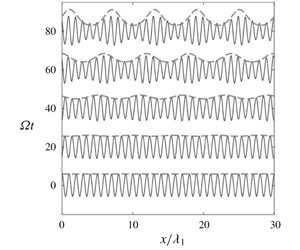
To obtain closed-form solutions of (5.12)–(5.13), Lewis et al. (Reference Lewis, Lake and Ko1974) adopted an asymptotic approach assuming $U_{0}/C=O(KA)\ll 1$ from (5.4) or, equivalently, $U_{0}/c_{g}\ll 1$ with $C/c_{g}=O(1)$ for the group resonance. While Lewis et al. (Reference Lewis, Lake and Ko1974) obtained an asymptotic solution in terms of the Heaviside function, which corresponds to imposing the boundary condition at the wavemaker, we here use an asymptotic solution of the initial value problem for (5.12)–(5.14) for the spatially periodic current given by (5.3) for its comparison with the numerical solutions of the Hamiltonian system (3.38). The explicit asymptotic solutions are given in appendix B.

At group resonance ($C=c_{g}$), the solutions of (5.12)–(5.14) for $k(x,t)$ and $a(x,t)$ valid to $O(\unicode[STIX]{x1D716})$ can be reduced, from (B 12)–(B 13), to

(5.15)$$\begin{eqnarray}\displaystyle & \displaystyle k(x,t)=k_{0}\,\text{exp}(-U_{0}Kt\sin \unicode[STIX]{x1D703}_{1}), & \displaystyle\end{eqnarray}$$

(5.16)$$\begin{eqnarray}\displaystyle & \displaystyle a(x,t)=a_{0}\,\text{exp}\left[-{\textstyle \frac{3}{4}}U_{0}Kt\sin \unicode[STIX]{x1D703}_{1}-{\textstyle \frac{1}{8}}U_{0}C(Kt)^{2}\cos \unicode[STIX]{x1D703}_{1}\right], & \displaystyle\end{eqnarray}$$

where $\unicode[STIX]{x1D703}_{1}=K(x-Ct)$. Then, the maxima and minima of $a$ and $k$ at a fixed time are given by

(5.17)$$\begin{eqnarray}\displaystyle & \displaystyle k_{max,min}=k_{0}\,\text{exp}\left[\pm (U_{0}/C)(\unicode[STIX]{x1D6FA}t)\right], & \displaystyle\end{eqnarray}$$

(5.18)$$\begin{eqnarray}\displaystyle & \displaystyle a_{max,min}=a_{0}\,\text{exp}\left[\pm {\textstyle \frac{3}{4}}(U_{0}/C)(\unicode[STIX]{x1D6FA}t)\left(1+{\textstyle \frac{2}{72}}(\unicode[STIX]{x1D6FA}t)^{2}\right)^{1/2}\right], & \displaystyle\end{eqnarray}$$

where $\unicode[STIX]{x1D6FA}=KC$ has been used and the plus and minus signs are chosen for the maxima and minima, respectively. Based on the linear modulation theory, both $|k_{max,min}|$ and $|a_{max,min}|$ increase with $t$. Then $a^{\ast }$ and $m^{\ast }$ defined by (5.1) with $m=ka$ can be found as

(5.19)$$\begin{eqnarray}\displaystyle & \displaystyle a^{\ast }(t)=\tanh [{\textstyle \frac{3}{4}}(U_{0}/C)(\unicode[STIX]{x1D6FA}t)(1+{\textstyle \frac{1}{36}}(\unicode[STIX]{x1D6FA}t)^{2})^{1/2}], & \displaystyle\end{eqnarray}$$

(5.20)$$\begin{eqnarray}\displaystyle & \displaystyle m^{\ast }(t)=\tanh [{\textstyle \frac{7}{4}}(U_{0}/C)(\unicode[STIX]{x1D6FA}t)(1+{\textstyle \frac{1}{196}}(\unicode[STIX]{x1D6FA}t)^{2})^{1/2}], & \displaystyle\end{eqnarray}$$

which are independent of the initial surface wave parameters and depend only on the internal wave steepness since $U_{0}/C=\unicode[STIX]{x1D70E}KA$, as shown in (5.4). While $k$ and $a$ increase in time exponentially, $a^{\ast }(t)$ and $m^{\ast }(t)$ approach 1 as $t\rightarrow \infty$.

For small $t$, or $\unicode[STIX]{x1D6FA}t\ll 1$, $a^{\ast }(t)$ and $m^{\ast }(t)$ can be approximated by

(5.21a,b)$$\begin{eqnarray}a^{\ast }(t)\simeq {\textstyle \frac{3}{4}}(U_{0}/C)(\unicode[STIX]{x1D6FA}t),\quad m^{\ast }(t)\simeq {\textstyle \frac{7}{4}}(U_{0}/C)(\unicode[STIX]{x1D6FA}t).\end{eqnarray}$$

Therefore, for small $\unicode[STIX]{x1D6FA}t$, or equivalently, small $Kx$ with $x=Ct$ , both $a^{\ast }(t)$ and $m^{\ast }(t)$ grow linearly in time and the growth rates increase with the internal wave steepness. In fact, Lewis et al. (Reference Lewis, Lake and Ko1974) noticed that the experimental data for different physical parameters collapse when $a^{\ast }/(U_{0}/C)$ and $m^{\ast }/(U_{0}/C)$ are used. This shows that their measurements were made over a relatively short distance or short time.

The exponential growths of $a(x,t)$ and $k(x,t)$ in time given by (5.15)–(5.16) are the result of the linear modulation theory for surface waves without considering the energy exchange with the internal wave. Therefore, the solutions given by (5.15)–(5.16) would be valid for $\unicode[STIX]{x1D6FA}t\ll O(1/\unicode[STIX]{x1D716})$. As time increases so that $\unicode[STIX]{x1D6FA}t=O(1/\unicode[STIX]{x1D716})$, the energy exchange through near-resonant triad interactions becomes important and the linear modulation theory is expected to less accurately describe the evolution of $a(x,t)$ and $k(x,t)$.

Another interesting feature in question is the location of the rough sea surface relative to the phase of the internal wave. Previously, its exact location for the long internal wave or the internal solitary wave has not been well understood as different field observations have been made (Gasparovic et al. Reference Gasparovic, Apel and Kasischke1988; Watson & Robinson Reference Watson and Robinson1990; Hwung et al. Reference Hwung, Yang and Shugan2009).

From (5.15)–(5.16), the local wave steepness $m=ka$ is given by

(5.22)$$\begin{eqnarray}m(x,t)=m_{0}\,\text{exp}[{\textstyle \frac{7}{4}}(U_{0}/C)(\unicode[STIX]{x1D6FA}t)(1+{\textstyle \frac{1}{196}}(\unicode[STIX]{x1D6FA}t)^{2})^{1/2}~\cos (\unicode[STIX]{x1D703}_{1}-\unicode[STIX]{x1D711})],\end{eqnarray}$$

where $m_{0}=k_{0}a_{0}$, and $\unicode[STIX]{x1D711}$ is defined as

(5.23)$$\begin{eqnarray}\unicode[STIX]{x1D711}=\tan ^{-1}\left(\frac{6}{\unicode[STIX]{x1D6FA}t}\right)+\unicode[STIX]{x03C0},\end{eqnarray}$$

which yields $\unicode[STIX]{x1D711}=3\unicode[STIX]{x03C0}/2$ for small $t$ and $\unicode[STIX]{x1D711}=\unicode[STIX]{x03C0}$ for large $t$. Then, from (5.22), as the maximum surface wave steepness is observed at $\unicode[STIX]{x1D703}_{1}=\unicode[STIX]{x1D711}$, its location can be found initially at up-crossings behind the crests of the internal wave, or at the points where the surface current given by (5.3) converges. On the other hand, as $t$ increases, the location of the maximum surface wave steepness is expected to be right above the internal wave troughs. Therefore, under the group resonance condition, steep surface waves are expected to appear at a point where the surface current converges only for a relatively short interaction period, but eventually appear right above the wave troughs. This conclusion, based on the linear modulation theory, will be further discussed later with the numerical solutions of the nonlinear Hamiltonian system.

6.1 Initialization for the experiment of Lewis, Lake & Ko (Reference Lewis, Lake and Ko1974)

After employing $h_{1}/h_{2}=10$ and $\unicode[STIX]{x1D70C}_{1}/\unicode[STIX]{x1D70C}_{2}=0.87$, the same as those in the experiment of Lewis et al. (Reference Lewis, Lake and Ko1974), we assume that the internal wave is a monochromatic wave (5.2) with $Kh_{1}=4.8$. Due to the periodic boundary conditions used in the pseudo-spectral method, a surface wavenumber identical to that used in the experiment is not admissible. As an integer number of surface wavelengths must be employed within an internal wavelength, the wavenumber of the initial monochromatic surface wave can be written as

(6.3)$$\begin{eqnarray}k_{1}=\unicode[STIX]{x1D705}K,\end{eqnarray}$$

where $\unicode[STIX]{x1D705}$ is an integer.

For case I, we choose $\unicode[STIX]{x1D705}=6$ so that the surface wavenumber $k_{1}h_{1}=28.8$, which is close to the wavenumber for group resonance, $k_{g}h_{1}\simeq 28.717$. Then, $C/c_{g}\simeq 1.009$. In comparison with $C/c_{g}=1\pm 0.02$ in Lewis et al. (Reference Lewis, Lake and Ko1974), our choice of $\unicode[STIX]{x1D705}=6$ gives $k_{1}$, which is within the error estimate of the experiment. For case II, $\unicode[STIX]{x1D705}=2$–14, giving a range of ratios for $C/c_{g}$ in the experiment.

In our numerical simulations, we use wave steepnesses identical to those used in the experiments: $\unicode[STIX]{x1D716}_{S}=0.055$ and $\unicode[STIX]{x1D716}_{I}=0.048$. While $\unicode[STIX]{x1D716}_{S}$ and $\unicode[STIX]{x1D716}_{\text{I}}$ are comparable, the amplitude of the internal wave is much greater than that of the surface wave: $A/a_{1}\simeq 5.24$. The initial conditions for $\unicode[STIX]{x1D701}_{1}$ and $\unicode[STIX]{x1D701}_{2}$ are given by a linear superposition of the surface (barotrophic) and internal (baroclinic) wave modes so that

(6.4a,b)$$\begin{eqnarray}\unicode[STIX]{x1D701}_{1}=a_{1}\cos (k_{1}x)+\unicode[STIX]{x1D6FD}_{3}^{-}A\cos (Kx),\quad \unicode[STIX]{x1D701}_{2}=\unicode[STIX]{x1D6FC}_{3}^{+}a_{1}\cos (k_{1}x)+A\cos (Kx),\end{eqnarray}$$

where $\unicode[STIX]{x1D6FC}_{3}^{+}=\unicode[STIX]{x1D6FC}_{3}(k_{1},\unicode[STIX]{x1D714}_{1})$ and $\unicode[STIX]{x1D6FD}_{3}^{-}=\unicode[STIX]{x1D6FD}_{3}(K,\unicode[STIX]{x1D6FA})$ with $\unicode[STIX]{x1D6FC}_{3}$ and $\unicode[STIX]{x1D6FD}_{3}$ given by (A 9) and (A 11), respectively. For the physical parameters in the experiment, $\unicode[STIX]{x1D6FC}_{3}^{+}\approx 0$ and $\unicode[STIX]{x1D6FD}_{3}^{-}=-7.18\times 10^{-4}$. Therefore, it can be safely assumed that the surface and interface displacements represent mostly those from the surface and internal wave modes, respectively. In addition, the linear relations in appendix A are used for $\unicode[STIX]{x1D6F9}_{1}$ and $\unicode[STIX]{x1D6F9}_{2}$.

Figure 6.

Snapshots of $(a)$ surface ($\unicode[STIX]{x1D701}_{1}$) and $(b)$ interface ($\unicode[STIX]{x1D701}_{2}$) displacements for case I with $C/c_{g}\simeq 1$. Solid curves: simulated wave displacements. Dashed curves: theoretical upper wave envelope from (5.16) in § 4. Dotted curves: the interface displacements shown in $(b)$ to display the relative phase between the surface and interface displacements. Notice that the vertical scales of the surface and interface displacements are different. At $t=0$ the amplitude ratio between the surface and internal wave modes is $A/a_{1}=5.24$. The horizontal axis is given by $x/\unicode[STIX]{x1D706}_{1}$, where $\unicode[STIX]{x1D706}_{1}$ is the surface wavelength.

The computational domain length and time are chosen to be sufficiently large for short surface waves to be fully evolved, typically, $5\unicode[STIX]{x1D6EC}$ and $12T$, respectively, where $\unicode[STIX]{x1D6EC}=2\unicode[STIX]{x03C0}/K$ and $T=2\unicode[STIX]{x03C0}/\unicode[STIX]{x1D6FA}$ are the wavelength and period of the internal wave, respectively. Convergence tests are performed for different choices of the computational domain length $L$ and the number of grid points per surface wavelength $M_{\unicode[STIX]{x1D701}_{1}}$ and their results will be discussed in § 6.2. The time step $\unicode[STIX]{x0394}t$ is chosen such that the Courant–Friedrichs–Lewy conditions are met: $c_{1}\unicode[STIX]{x0394}t/\unicode[STIX]{x0394}x\ll 1$ and $C\unicode[STIX]{x0394}t/\unicode[STIX]{x0394}x\ll 1$, where $\unicode[STIX]{x0394}x=L/M$ while $c_{1}=\unicode[STIX]{x1D714}_{1}/k_{1}$ and $C=\unicode[STIX]{x1D6FA}/K$ are the phase speeds of the surface and internal waves, respectively.

As the numerical model solves initial value problems with periodic boundary conditions, it computes the temporal evolution of the surface and internal waves. For comparison with the measurements of $a^{\ast }$ and $m^{\ast }$, the temporal evolution of the surface wave envelope needs to be transformed to the corresponding spatial evolution, or vice versa. Here, the transformation with the group velocity of the surface wave is adopted, i.e. $x=c_{g}t$, and the interaction distance measured with respect to $K$ becomes $Kx=Kc_{g}t~=KCt=\unicode[STIX]{x1D6FA}t$ when $C/c_{g}=1$.

6.2 Comparison with experiments of Lewis et al. (Reference Lewis, Lake and Ko1974)

Figure 6 shows the time evolution of the surface and internal wave displacements for case I. From figure 6(a), it is observed that the simulated surface wave is modulated by the internal wave and evolves into almost spatially periodic wave packets. When it is compared with the numerical solution, the linear modulation theory in § 5.2 predicts accurately the amplitude of the envelope, but, for instance, around $\unicode[STIX]{x1D6FA}t\approx 80$, starts to overpredict the surface modulation. From figure 6(b), a slight change in the internal wave profile is observed relative to the initial profile. Slightly steep crests and flattened troughs are observed. This change could be attributed to the effect of the second-order nonlinearity in the Hamiltonian system on the internal wave. This nonlinear behaviour seems to appear due to the shallowness of the lower layer, where the dimensionless internal wavenumber $Kh_{2}=0.48$ or $h_{2}/\unicode[STIX]{x1D6EC}=0.076$. In the simulations for larger values of $Kh_{2}$, the internal wave of the same steepness shows little changes in its profile.

As shown in figure 6(a), the maximum surface wave steepness is observed approximately right above the internal wave troughs. This is consistent with the theoretical prediction discussed in § 5.2. Therefore, while the linear modulation theory starts to deviate from the numerical solution (and the observation) at $\unicode[STIX]{x1D6FA}t\approx 80$, it predicts well the location of steep surface area.

Figure 7 shows the numerical results for the amplitude modulation $a^{\ast }$ given by (5.1) as a function of $\unicode[STIX]{x1D6FA}t$ for varying two numerical parameters: $M_{\unicode[STIX]{x1D701}_{1}}$ and $L$, which are the number of spatial grid points per surface wavelength and the computational domain length, respectively. The numerical data for $a^{\ast }$ are shown scattered for fixed values of $M_{\unicode[STIX]{x1D701}_{1}}$ and $L$. For the convergence test, the scattered numerical results are smoothed with 50 iterations of a three-point moving average. The solid black and grey curves show smoothed numerical data for various choices of $M_{\unicode[STIX]{x1D701}_{1}}$ and $L$. This convergence test shows that the choice of $M_{\unicode[STIX]{x1D701}_{1}}=32$ and $L=5\unicode[STIX]{x1D6EC}$, employed in figure 6, is sufficient to capture the amplitude modulation described by $a^{\ast }$.

Figure 7.

Convergence of amplitude modulation, $a^{\ast }$, as a function of $\unicode[STIX]{x1D6FA}t$ for case I for different values of the number of spatial grid points per surface wavelength $M_{\unicode[STIX]{x1D701}_{1}}$ and the computational domain length $L$. The numerical data (dots) are smoothed with 50 iterations of a three-point moving average.

Figure 8.

Normalized amplitude and slope modulation, $a^{\ast }$ and $m^{\ast }$ defined by (5.1), as functions of $\unicode[STIX]{x1D6FA}t$ for case I. Open circles: experiment; dots: simulation employing $\unicode[STIX]{x1D705}=6$ in (6.3); dashed curves: smoothed numerical solutions; solid curves: linear modulation theory of Lewis et al. (Reference Lewis, Lake and Ko1974) given by (B 15)–(B 16); dash–dotted curves: linear modulation theory given by (5.19)–(5.20).

Figure 8 shows the amplitude $a^{\ast }$ and slope $m^{\ast }~\text{m}$odulations for case I, as functions of $\unicode[STIX]{x1D6FA}t$, from the experiment, simulation and linear modulation theory. The experimental data shown by open circles are extracted from figures 12 and 13 on page 796 in Lewis et al. (Reference Lewis, Lake and Ko1974) and are normalized by $U_{0}/C$. As shown in (5.21), this normalization makes their experimental data for different physical parameters collapse almost onto a single curve over a short interaction distance or time. The two theoretical solutions discussed in appendix B, corresponding to those of the boundary and initial value problems, respectively, are also presented, but show little difference. This confirms that the transformation from the temporal evolution of the surface wave to the spatial evolution using its group velocity is reliable. Therefore, hereafter, only the asymptotic solutions in § 5.2 will be presented.

As shown in figure 8, the experimental and numerical data are in good agreement, although relatively minor discrepancies are observed. On the other hand, the linear modulation theory agrees with the experimental and numerical data approximately up to $\unicode[STIX]{x1D6FA}t=30$, but clearly overestimates the surface wave modulation approximately for $\unicode[STIX]{x1D6FA}t>40$. This observation indicates that the linear modulation theory fails to describe the modulation after the initial exponential growth and needs to be modified to include nonlinear effects, as discussed in the following section.

Figure 9.

Normalized amplitude and slope modulation, $a^{\ast }$ and $m^{\ast }$, from (5.1) as functions of $C/c_{g}$ at $Kx=\unicode[STIX]{x1D6FA}t=43$ for case II. Open circles: experiment; dots: simulations employing $\unicode[STIX]{x1D705}=2$–14 in (6.3); dash–dotted curves: linear modulation theory given by (B 12)–(B 13).

To investigate how effective the group resonance mechanism is for the modulation of short surface waves, we numerically study case II of Lewis et al. (Reference Lewis, Lake and Ko1974). Figure 9 shows $a^{\ast }$ and $m^{\ast }$ as functions of $C/c_{g}$ at a fixed propagation distance of $Kx=\unicode[STIX]{x1D6FA}t=43$, chosen in their experiment. The experimental data are extracted from figures 14 and 15 on page 797–798 in Lewis et al. (Reference Lewis, Lake and Ko1974). From figure 9, it is observed experimentally, numerically and theoretically that the largest amplitude and slope modulation appear under the group resonance condition, $C/c_{g}=1$. Notice that, due to the periodic boundary conditions of our numerical model, only a few data points are available through $\unicode[STIX]{x1D705}=2$–14 in (6.3). Nevertheless, the limited numbers of data points reveal the trend of the experiment and theory.

Figure 10.

Normalized amplitude and slope modulation, $a^{\ast }$ and $m^{\ast }$ defined by (5.1), as functions of $\unicode[STIX]{x1D6FA}t$ for case I for a longer period than the experiment of Lewis et al. (Reference Lewis, Lake and Ko1974). Open circles: experiment; dots: simulation employing $\unicode[STIX]{x1D705}=6$ in (6.3); dashed curves: smoothed numerical solutions; dash–dotted curves: linear modulation theory given by (5.19)–(5.20).

Figure 11.

Numerical solutions of the Hamiltonian system for the amplitudes of surface and internal waves for internal wave steepness $\unicode[STIX]{x1D716}_{I}=0.048$ corresponding to case I of the experiments. $(a)$ Internal wave amplitude $A$. $(b)$ Surface wave amplitude $a_{1}$. (c,d) Near-resonant surface wave amplitudes $a_{n+}$ (dashed curves) and $a_{n-}$ (dash–dotted curves) for $n=2,\,3$. The amplitudes are normalized by the initial surface wave amplitude $a_{0}=a_{1}(t=0)$.

6.3 Evolution of surface waves over a longer period

Figure 10 shows $a^{\ast }$ and $m^{\ast }$ as functions of $\unicode[STIX]{x1D6FA}t$ for case I for a longer period than that displayed in figure 8. It is observed that, after the initial exponential growth, the modulation reaches a maximum at $\unicode[STIX]{x1D6FA}t\approx$ 90 before it starts to oscillate. This implies that the $k_{1}$ wave is modulated and starts to exchange energy with its sidebands through near-resonant wave interactions, as discussed in Alam (Reference Alam2012). In Lewis et al. (Reference Lewis, Lake and Ko1974), as the measurements were made over a short distance, the initial growth of sidebands were reasonably well described by the linear modulation theory and no energy flow back to the carrier wave was observed.

Figure 11 shows the time evolution of $A$, $a_{1}$ and $a_{n\pm }$$(n=2,3)$ that are the wave amplitudes of wavenumbers $K$, $k_{1}$ and $k_{n_{\pm }}=k_{1}\pm (n-1)K$. These amplitudes are computed from the moduli of the numerical surface and interface displacements $|\hat{\unicode[STIX]{x1D701}}_{1}(k,t)|$ and $|\hat{\unicode[STIX]{x1D701}}_{2}(k,t)|$, respectively, which have been shown to be good approximations to the amplitudes of the surface and internal wave modes, as pointed out in (6.4). The amplitudes are normalized by the initial amplitude of the surface wave $a_{0}=a_{1}(t=0)$ of $\unicode[STIX]{x1D701}_{1}$.

From figure 11(a), the internal wave amplitude $A$ whose magnitude is approximately 5 times higher than $a_{1}$ is observed to oscillate with a relatively small amplitude. While the source of this oscillation of a relatively short period (but much greater than $2\unicode[STIX]{x03C0}/\unicode[STIX]{x1D6FA}$) is unclear, it seems to be the effect of the shallow lower layer $(Kh_{2}=0.48)$ as the simulations with deeper lower layers do not exhibit such an oscillation. Unfortunately, no measurements of internal waves were reported in Lewis et al. (Reference Lewis, Lake and Ko1974).

In the meantime, it is observed from figure 11(b) that $a_{1}$ also oscillates with a small amplitude, but with a much longer period than the oscillation period of $A$. Initially $a_{1}$ decreases and reaches its minimum around $\unicode[STIX]{x1D6FA}t\approx 90$ indicating that energy is transferred to neighbouring wave components that satisfy the near-resonant conditions. As can be seen from figure 11(c), $a_{2_{\pm }}$, which are the third members of the primary resonant triads, receive energies from the waves of $A$ and $a_{1}$ to grow from zero and then decay by returning their energies back to $a_{1}$ and $A$. This process repeats with distinct recurrence periods: $\unicode[STIX]{x1D6FA}t\approx 150$ for $a_{2_{+}}$ and $\unicode[STIX]{x1D6FA}t\approx 210$ for $a_{2_{-}}$. When $a_{2_{\pm }}$ are close to their maxima around $\unicode[STIX]{x1D6FA}t\approx$ 90, the surface wave modulation measured by $a^{\ast }$ and $m^{\ast }$ reaches its maximum, as shown in figure 10. Similarly to Alam (Reference Alam2012), $a_{3_{\pm }}$ are also excited by successive interactions, but their amplitudes observed in figure 11(d) are much smaller than those of the primary resonant triads, e.g. approximately one order of magnitude smaller than $a_{2_{\pm }}$.

Unlike the resonant interaction studied by Alam (Reference Alam2012) (also considered in § 4.2), the interactions are relatively weak for the parameters used in the experiment of Lewis et al. (Reference Lewis, Lake and Ko1974). For example, the variation of the amplitude of the $k_{1}$ wave during the primary triad interaction with $k_{2_{\pm }}$ is much smaller than that observed in Alam (Reference Alam2012). Furthermore the amplitudes of the sidebands excited by the successive interactions ($k_{n_{\pm }}$ for $n\geqslant 3$) are much smaller than those in Alam (Reference Alam2012). Although they are necessary to accurately describe the surface wave field, the sidebands excited by successive interactions are less important for the parameters in the experiment of Lewis et al. (Reference Lewis, Lake and Ko1974).