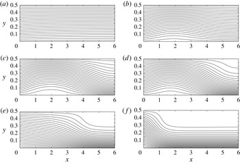
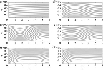
1. Introduction
The dynamics of swirling flows in a pipe, specifically at high levels of rotation, are dominated by flow instabilities and the vortex-breakdown phenomenon (see Sarpkaya Reference Sarpkaya1971, Reference Sarpkaya1974; Faler & Leibovich Reference Faler and Leibovich1977; Garg & Leibovich Reference Garg and Leibovich1979; Leibovich Reference Leibovich1984; Brucker & Althaus Reference Brucker and Althaus1995; Mattner, Joubert & Chong Reference Mattner, Joubert and Chong2002; Liang & Maxworthy Reference Liang and Maxworthy2005). Most of the experimental studies focus on flows with narrow to medium-size vortical cores that may be represented by the Lamb–Oseen or the
 $Q$
-vortex models, or similar models. In stationary pipes, at low-Reynolds-number flows,
 $\mathit{Re}<10^{4}$
, the instabilities range from helical waves to the two major types of breakdown, the axisymmetric bubble and the spiral breakdown. At higher
 $\mathit{Re}$
,
 $\mathit{Re}>50\,000$
, the experiments show that the axisymmetric breakdown zone is long, parabolic in shape, open downstream and dominates the flow dynamics (Sarpkaya Reference Sarpkaya1995). High-frequency spiral waves appear inside these breakdown zones. Currently, there is no general consensus in the literature that vortex breakdown describes a single phenomenon or that there is a unique mechanism of the breakdown process.
Several theories have been advanced over the years to explain various aspects or mechanisms of the vortex-breakdown phenomenon, including the studies by Benjamin (Reference Benjamin1962, Reference Benjamin1967), Randall & Leibovich (Reference Randall and Leibovich1973) and Leibovich & Kribus (Reference Leibovich and Kribus1990), who investigated the dynamics of standing or travelling nonlinear waves on swirling flows in an infinitely long pipe. We note that the case of a flow in an infinitely long straight pipe pertains to a translational invariance and that such an entity does not exist in practice. The addition of a localized contraction to an infinitely long pipe can eliminate this invariance and generate large-amplitude travelling waves or standing waves that may resemble breakdown states (see Grimshaw & Yi Reference Grimshaw and Yi1993; Hanazaki Reference Hanazaki1996). However, these studies do not allow an interaction between the waves and the inlet and outlet states. On the other hand, the studies of Beran & Culick (Reference Beran and Culick1992), Beran (Reference Beran1994), Lopez (Reference Lopez1994), Wang & Rusak (Reference Wang and Rusak1996a ,Reference Wang and Rusak b , Reference Wang and Rusak1997), Snyder & Spall (Reference Snyder and Spall2000), Rusak & Judd (Reference Rusak and Judd2001), Gallaire & Chomaz (Reference Gallaire and Chomaz2004), Leclaire & Sipp (Reference Leclaire and Sipp2010) and Rusak et al. (Reference Rusak, Wang, Xu and Taylor2012) examined the dynamics of swirling flows in a finite-length pipe with no translational invariance. Such a setting is completely different from the case of an infinitely long pipe flow, allows an interaction of the flow in the bulk with the inlet and outlet states, and may better represent the flows in the experimental apparatuses.
The pioneering approach of Benjamin (Reference Benjamin1962) revealed the existence of a special swirl ratio
 ${\it\omega}_{B}$
at which an infinitesimally small, long, axisymmetric standing wave may appear on a columnar swirling flow in an infinitely long pipe. Using this property, Benjamin (Reference Benjamin1962) attributed dynamical characteristics to a swirling flow; flows with swirl ratios
 $0\leqslant {\it\omega}<{\it\omega}_{B}$
can sustain only downstream-travelling perturbations and are termed ‘supercritical states’. On the other hand, flows with
 ${\it\omega}>{\it\omega}_{B}$
can exhibit perturbations that propagate both upstream and downstream and are termed ‘subcritical states’. Benjamin’s scenario of the axisymmetric breakdown state is a finite standing jump transition from an upstream supercritical columnar state to a conjugate downstream subcritical columnar state that is associated with upstream-propagating waves when the jump is weak or with a total head loss through the jump when the jump is strong. This approach is analogous to the hydraulic jump phenomenon that occurs in shallow water. Based on the classical vortex stability theory known at his time, Benjamin (Reference Benjamin1962) speculated that the breakdown state is not a manifestation of the loss of stability of the upstream flow as a base columnar state. His theory tried to overcome this difficulty.
The classical vortex stability theory (Kelvin Reference Kelvin1880; Rayleigh Reference Rayleigh1916; Synge Reference Synge1933; Howard & Gupta Reference Howard and Gupta1962; Leibovich & Stewartson Reference Leibovich and Stewartson1983) used axial normal periodic modes on a swirling flow and showed that the columnar flow stability is directly related to the monotonicity of the flow circulation function. Such a study, however, is valid only for a columnar swirling flow in an infinitely long pipe or in a finite-length pipe with periodic boundary conditions that necessarily preserve a translational invariance. This limitation has been overlooked for a long time and the Rayleigh stability criterion was thought to be applicable for any vortex flow in a pipe. The stability analysis of Wang & Rusak (Reference Wang and Rusak1996a ) was the first to reveal this crucial limitation of the classical stability theory. They proposed a completely different mode analysis that is able to describe the physics of swirling flows in a finite-length pipe where the translational invariance does not exist, and this analysis is consistent with a swirling flow behaviour in the experimental apparatuses mentioned above.
The physical model of Wang & Rusak (Reference Wang and Rusak1996a
) consists of a swirling flow in a straight, finite-length pipe that can be generated by a fixed-in-time and fixed-in-place vortex generator ahead of the pipe at a continuous and smooth operation. The generator forms, at the pipe inlet, steady and smooth profiles of the axial and circumferential velocity components and of the azimuthal vorticity. A zero radial velocity state is set at the pipe outlet. The mode analysis of this setting gives rise to a new set of eigenmodes that are completely different from the classical normal modes in an infinitely long pipe. All the modes are asymptotically stable when
 ${\it\omega}$
is less than a critical swirl level
 ${\it\omega}_{1}$
(i.e. a modified level of Benjamin’s special swirl
 ${\it\omega}_{B}$
due to the pipe length
 $L$
). The least stable of these modes becomes neutral at
 ${\it\omega}={\it\omega}_{1}$
, and becomes unstable when
 ${\it\omega}>{\it\omega}_{1}$
, making the critical columnar state at
 ${\it\omega}={\it\omega}_{1}$
a point of exchange of flow stability. Wang & Rusak (Reference Wang and Rusak1997) showed that this state is also an inflection point of the variational energy integral
 $\mathscr{E}$
that governs the axisymmetric steady flow problem. Additional instability modes appear in sequence as
 ${\it\omega}$
is further increased above
 ${\it\omega}_{1}$
(Rusak et al.
Reference Rusak, Wang, Xu and Taylor2012). The instability process at
 ${\it\omega}>{\it\omega}_{1}$
initiates the linear growth of perturbations away from the columnar state and is followed by a faster-than-exponential process where the growth rate increases with the perturbation size. This process includes the interaction between steepening effects, sizable dispersion effects and the inlet–outlet conditions that may be described by a nonlinear Korteweg–de Vries (KdV) equation in a finite-length pipe with non-periodic inlet–outlet conditions. Rusak et al. (Reference Rusak, Wang, Xu and Taylor2012) quantitatively captured this process by numerical flow simulations. They described the evolution of the growing perturbations to a breakdown state that consists of the incoming swirling flow expanding around a large and open near-stagnation centreline zone, as predicted by the theoretical study of Wang & Rusak (Reference Wang and Rusak1997). The branch of breakdown states starts from another critical state at
 ${\it\omega}={\it\omega}_{0}<{\it\omega}_{1}$
. The vortex-breakdown process is a manifestation of the flow nonlinear instability when
 ${\it\omega}>{\it\omega}_{0}$
and the flow linear instability when
 ${\it\omega}>{\it\omega}_{1}$
. We note that the swirling flow in a finite-length pipe is more general in its dynamical behaviour and does not follow the shallow-water model and its hydraulic jump state as a limit case. We also note that the nonlinear KdV equation was used by Randall & Leibovich (Reference Randall and Leibovich1973), Grimshaw & Yi (Reference Grimshaw and Yi1993) and Hanazaki (Reference Hanazaki1996) to study the dynamics of nonlinear waves on swirling flows (including the solid-body rotation) in an infinitely long pipe. However, as mentioned before, this forms a dynamical situation of a swirling flow in a pipe that may describe the transient dynamics of localized perturbations before they interact with the inlet and outlet states.
In addition, the review of the literature shows that there is no strong experimental or numerical evidence that the axisymmetric breakdown state is indeed a columnar–columnar, standing jump transition. Instead, the experimental data (Sarpkaya Reference Sarpkaya1971, Reference Sarpkaya1974, Reference Sarpkaya1995; Garg & Leibovich Reference Garg and Leibovich1979; Mattner et al.
Reference Mattner, Joubert and Chong2002; Liang & Maxworthy Reference Liang and Maxworthy2005) and flow computations (Beran & Culick Reference Beran and Culick1992; Beran Reference Beran1994; Lopez Reference Lopez1994; Darmofal Reference Darmofal1996; Ruith et al.
Reference Ruith, Chen, Meiburg and Maxworthy2003; Meliga & Gallaire Reference Meliga and Gallaire2011; Rusak et al.
Reference Rusak, Wang, Xu and Taylor2012) show that it is a smooth radial expansion of the upstream flow around a large-scale, nearly stagnant breakdown zone, which must include both axial and radial dispersion. These observations suggest that the breakdown state is not a finite jump transition as proposed by Benjamin (Reference Benjamin1962), but a minimum-path transition along a finite-length domain between a given inlet vortex state and a related downstream state with a centreline stagnation zone. For a given inlet vortex profile, the minimum-path transition is forming a state that minimizes the energy integral
 $\mathscr{E}$
over the whole flow domain. This spatial transition occurs along axial and radial scales that are of the order of the core size (or less) when the vortex core is large, and of larger scales when the vortex core is of a small size: see details in the global analysis of Wang & Rusak (Reference Wang and Rusak1997). The breakdown state in such a case is different from Benjamin’s model of breakdown. The theory is supported by the numerical simulations of Rusak et al. (Reference Rusak, Wang, Xu and Taylor2012), the analysis of experimental data in Rusak, Whiting & Wang (Reference Rusak, Whiting and Wang1998) and Rusak & Lamb (Reference Rusak and Lamb1999), and the experimental data reported in Mattner et al. (Reference Mattner, Joubert and Chong2002).
A relevant comprehensive study of swirling flows with large core sizes and axial jets has been conducted by Leclaire & Sipp (Reference Leclaire and Sipp2010). They investigated the influence of two possible inlet conditions. The first is the same azimuthal vorticity inlet condition that we use, which allows the radial velocity to change along the inlet. The second is an inlet state with a zero radial velocity, which allows the azimuthal vorticity to change along the inlet. They also used various profiles of swirling jets at the inlet that are modified profiles of the solid-body rotation with a uniform axial velocity. They determined for the first time a range of base flow parameters where the bifurcation of steady states from the first critical swirl ratio exhibits a different orientation with respect to the established transcritical bifurcation found in the Lamb–Oseen vortex (see their figure 3). They also identified special limit states where a stagnation point appears along either the pipe centreline or the pipe wall, indicating the possible appearance of breakdown and wall-separation states. The extension of branches of such states that develop out of the limit states can be established by methods that are presented in this paper.
In this paper, we study the incompressible and inviscid axisymmetric dynamics of a base solid-body rotation flow with a uniform axial velocity in a rotating, finite-length, straight circular pipe. This case provides a basic study of the behaviour of a swirling flow with large vortical core sizes. We find that the dynamics of a base solid-body rotation flow with a uniform axial velocity are strikingly different from those of the Lamb–Oseen vortices with narrow to medium vortical core sizes. According to Wang & Rusak (Reference Wang and Rusak1997), the steady flow case with an inlet Lamb–Oseen vortex is governed by a nonlinear Squire–Long equation, and exhibits a transcritical bifurcation at its
 ${\it\omega}_{1}$
and a fold swirl level at another critical swirl
 ${\it\omega}_{0}$
(
 ${<}{\it\omega}_{1}$
), from which a branch of vortex-breakdown states bifurcates. On the other hand, the steady case of an inlet solid-body rotation flow is governed by a linear Squire–Long equation and exhibits a jump bifurcation at its
 ${\it\omega}_{1}$
that also eliminates the fold state at
 ${\it\omega}_{0}$
. Moreover, from a dynamical perspective, the Lamb–Oseen vortex case shows the appearance of faster-than-exponential growing perturbations leading to vortex-breakdown states when
 ${\it\omega}>{\it\omega}_{0}$
, while the solid-body rotation case is dominated by a linear dynamics of the growth of perturbations (see also Rusak et al.
Reference Rusak, Wang, Xu and Taylor2012). Also note that the classical stability theory of a solid-body rotation flow with periodic inlet–outlet conditions lacks any instability mechanism (see Kelvin Reference Kelvin1880), as well as any transient or nonlinear growth mechanisms of perturbations (see Wang Reference Wang2009). Therefore, this flow cannot allow the appearance of breakdown or wall-separation zones as an evolution from an initially slightly perturbed columnar flow in an infinitely long pipe. The breakdown scenario of Benjamin cannot appear out of a dynamical process of flow perturbations. Moreover, the Wang & Rusak (Reference Wang and Rusak1996a
) instability of the solid-body rotation in a finite-length pipe is the only mechanism that can sustain the growth of perturbations in the flow. This flow cannot generate any growth of perturbations in the bulk, and the instability occurs only through the interaction between the perturbation in the bulk and the inlet and outlet states (see Gallaire & Chomaz Reference Gallaire and Chomaz2004; Wang & Rusak Reference Wang and Rusak2011).
In addition, the present flow study provides a case study that is analysed in this paper by analytical techniques to obtain an understanding of this distinctive flow dynamics. The study reveals the exact range of existence of a unique solution and the ranges of existence of multiple solutions of the steady-state flow problem, including global and local minimizer states and min–max states of the variational energy functional
 $\mathscr{E}$
that governs the steady flow problem. As a result, the flow dynamics as related to minimizer and min–max states can be described. Among the equilibrium states are axisymmetric vortex-breakdown states and wall-separation states that are characterized.
The possible coexistence of steady axisymmetric breakdown and wall-separation states in viscous swirling flows was first suggested by the analytical study of Lavan, Nielsen & Fejer (Reference Lavan, Nielsen and Fejer1969), and the numerical studies of Crane & Burley (Reference Crane and Burley1976) and Silvester, Thatcher & Duthie (Reference Silvester, Thatcher and Duthie1984). Rusak & Meder (Reference Rusak and Meder2004) and Leclaire, Sipp & Jacquin (Reference Leclaire, Sipp and Jacquin2007) found such states in inviscid swirling flows with large vortical cores in contracting pipes. Leclaire & Sipp (Reference Leclaire and Sipp2010) also indicated the possible existence of such states in inviscid swirling flows in a straight circular pipe. These states may also be found in vortex flows with medium- to small-size cores, but only when the swirl is sufficiently high and far above the critical level
 ${\it\omega}_{1}$
. Even then, it is rare that they are reached through the dynamics of perturbed columnar flows, because of a different and more complicated bifurcation manifold of steady states for flows other than the solid-body rotation (Rusak et al.
Reference Rusak, Wang, Xu and Taylor2012). This may be the reason why wall-separation states were never observed in the experiments of Sarpkaya (Reference Sarpkaya1971, Reference Sarpkaya1974, Reference Sarpkaya1995) and Garg & Leibovich (Reference Garg and Leibovich1979), where the core sizes of the vortices were relatively narrow. To support the relevance of our study, we refer to the experimental results of Mattner et al. (Reference Mattner, Joubert and Chong2002) concerning relatively large-core vortex flows, which may indicate, in their figure 21, evidence for the appearance of such states at high swirl levels. We also refer to the recent paper by Dennis, Seraudie & Poole (Reference Dennis, Seraudie and Poole2014), which is probably the first experiment to demonstrate the coexistence of axisymmetric wall-separation states and axisymmetric vortex-breakdown states at the same swirl level (i.e. above-critical) in a rotating pipe setting. Note that these experiments did not show any hysteresis loop between the wall-separation and breakdown states. This indicates that each one of these states is an attractor of flow dynamics, depending on the initial perturbations. Our present paper also shows that the appearance of the wall-separation zones has an equal chance of occurring as the evolution to vortex-breakdown zones and that there is no hysteresis loop between these states. The present results should be investigated in further detailed experimental studies to verify the theoretical predictions of flow dynamics and the evolution to both breakdown and wall-separation states.
The outline of the paper is as follows. The mathematical model problem is formulated in § 2. Section 3 gives a complete analysis of the global bifurcation of steady flow states when the inlet flow is solid-body rotation and swirl ranges from 0 to above
 ${\it\omega}_{1}$
. We also describe the expected dynamics of perturbed columnar flows. Section 4 provides numerically simulated representative examples of flow dynamics at various swirl ratios, starting from various initial perturbations. The simulations complete the information about the bifurcation diagram that cannot be obtained through the analytical techniques, as well as supporting the theoretical predictions. Section 5 summarizes the conclusions of this study.
2. The mathematical model
We consider an incompressible, inviscid and axisymmetric, swirling flow in a rotating, straight, finite-length, circular pipe. Cylindrical coordinates
 $(r,{\it\theta},x)$
are used, where
 $(u,v,w)$
are the radial, azimuthal and axial velocity components, respectively. The axial and radial distances are scaled with the pipe radius and the pipe non-dimensional length is
 $L$
. The velocity components are scaled with the characteristic axial speed entering the pipe. The time
 $t$
is scaled with the ratio of pipe radius to inlet characteristic speed. Let
 $y=r^{2}/2$
. By virtue of the axisymmetry, a stream function
 ${\it\psi}(x,y,t)$
can be defined such that
 $u=-{\it\psi}_{x}/\sqrt{2y}$
and
 $w={\it\psi}_{y}$
. The reduced form of the azimuthal vorticity is
 ${\it\chi}=-({\it\psi}_{yy}+{\it\psi}_{xx}/2y)$
(where the azimuthal vorticity is
 ${\it\eta}=\sqrt{2y}{\it\chi}$
). The circulation function is
 $K=rv=\sqrt{2y}v$
. The equations that relate the evolution of
 ${\it\psi}(x,y,t)$
,
 ${\it\chi}(x,y,t)$
and
 $K(x,y,t)$
are as follows:
 $$\begin{eqnarray}\displaystyle \left.\begin{array}{@{}l@{}}K_{t}+{\it\psi}_{y}K_{x}-{\it\psi}_{x}K_{y}=0,\\ {\it\chi}_{t}+{\it\psi}_{y}{\it\chi}_{x}-{\it\psi}_{x}{\it\chi}_{y}=\displaystyle \frac{1}{4y^{2}}(K^{2})_{x}.\end{array}\right\} & & \displaystyle\end{eqnarray}$$
The first equation in (2.1) is the transport equation of flow circulation along a path line. The second equation describes the interaction between the convection of the reduced azimuthal vorticity
 ${\it\chi}$
along a path line and vorticity stretching with the axial gradient of the circulation. The latter effect is swirl dependent and generates swirl-driven waves that can propagate either downstream or upstream, either along the pipe centreline or along the pipe wall, and interact with the pipe inlet and outlet within a finite time to grow and establish flow states with separation zones.
The system (2.1) is subjected to certain boundary conditions that reflect a physical setting of a flow in a pipe generated by a vortex generator at a steady, continuous and smooth operation ahead of the pipe. In the present study, we focus on a special setting where the inlet profile is a steady solid-body rotating flow with a uniform axial velocity; i.e. for all time
 $t\geqslant 0$
and for
 $0\leqslant y\leqslant \frac{1}{2}$
,
 ${\it\psi}(0,y,t)={\it\psi}_{0}(\,y)=y$
and
 $K(0,y,t)=2{\it\omega}y$
. Here,
 ${\it\omega}\geqslant 0$
is the inlet flow swirl ratio. The reduced azimuthal vorticity at the inlet is set to be
 ${\it\chi}(0,y,t)=-{\it\psi}_{0yy}=0$
or, equivalently,
 ${\it\psi}_{xx}(0,y,t)=0$
along the inlet for all time
 $t\geqslant 0$
and
 $0\leqslant y\leqslant \frac{1}{2}$
. Note that the radial velocity along the inlet is not fixed and may change in time in response to the upstream propagation of waves in the pipe.
These inlet conditions, and specifically the fixed vorticity inlet condition, may represent the nature of the rolled up vortex flow behind a vortex generator that consists of a system of fixed-in-time and fixed-in-space guiding (turning) vanes with a conical centrebody. We note that the experimental studies of Sarpkaya (Reference Sarpkaya1971, Reference Sarpkaya1974, Reference Sarpkaya1995), Garg & Leibovich (Reference Garg and Leibovich1979), Brucker & Althaus (Reference Brucker and Althaus1995), Mattner et al. (Reference Mattner, Joubert and Chong2002) and Umeh et al. (Reference Umeh, Rusak, Gutmark, Villalva and Cha2010) used guiding vanes to generate an inlet circumferential velocity that is represented by the
 $Q$
-vortex model with either small or large core sizes. In the limit, and through a careful fine design of the turning vanes, the inlet circumferential velocity may approach the solid-body rotation flow (which is a special case of a vortex flow with a core size that is the same as the pipe radius). Also, the inlet axial velocity in these experiments is not uniform; usually, it is a jet-like flow. This matches the nearly constant total head that characterizes the flow through the passive guiding vanes. Yet, an inlet uniform axial velocity may be generated by adding special flow resistances through the guiding vanes. We also refer to Snyder & Spall (Reference Snyder and Spall2000), who demonstrated that a numerical simulation of the flow in a pipe including the guiding vanes system ahead of it and a simulation of the flow in the pipe alone, with fixed-in-time inlet axial and circumferential velocity profiles taken from the full apparatus simulation, give the same results and resemble the experiments of Sarpkaya (Reference Sarpkaya1974). This result further supports the present approach of setting the inlet conditions.
The outlet boundary condition is described by a zero radial velocity (parallel flow) all along the outlet, i.e. for all time
 $t\geqslant 0$
,
 ${\it\psi}_{x}(L,y,t)=0$
for
 $0\leqslant y\leqslant \frac{1}{2}$
. This condition is supported by the experimental data shown in Umeh et al. (Reference Umeh, Rusak, Gutmark, Villalva and Cha2010), where the mean swirling flow has established a parallel flow state after several radii from the inlet. This is also supported by the simulations of Meliga & Gallaire (Reference Meliga and Gallaire2011).
The symmetry condition is imposed along the pipe centreline, i.e.
 ${\it\psi}(x,0,t)=0$
for
 $0\leqslant x\leqslant L$
and for all time
 $t\geqslant 0$
. Along the pipe wall at
 $y=\frac{1}{2}$
, the stream function is fixed;
 ${\it\psi}(x,\frac{1}{2},t)=\frac{1}{2}$
for
 $0\leqslant x\leqslant L$
and all time
 $t\geqslant 0$
, to describe the total volumetric flux across the pipe and the flow tangency along the pipe wall. This condition also leads, for all time
 $t\geqslant 0$
, to a constant value of the circulation function along the wall. Therefore, the flow circumferential velocity on the pipe wall matches with the pipe wall rotational speed and thereby does not generate a wall boundary layer of the circumferential velocity. Also, in the case of a finite-length pipe (that is shorter than the entrance length to a fully developed viscous flow) and at a sufficiently high-Reynolds-number flow, the axial flow boundary layer is thin all along the pipe and has only a weak effect on the axial velocity field.
We emphasize that this set of boundary conditions is consistent with the transport equations (2.1) for the circulation and the azimuthal vorticity, and with the Poisson equation for the stream function in terms of
 ${\it\chi}$
. They form a well-posed mathematical problem of the flow dynamics in the pipe. We note that any well-posed mathematical problem corresponds to a physical set-up that in principle can be realized as suggested above. In addition, the inlet vorticity condition provides a base case study, where the total head and circulation functions entering the pipe are the same for multiple possible steady states in the pipe at the same swirl and with the same boundary conditions. This condition also supports the existence of a branch of columnar flow states in the pipe for every swirl level
 ${\it\omega}$
, from which various branches of non-columnar states bifurcate as
 ${\it\omega}$
is increased. The effect of a steady, non-zero inlet azimuthal vorticity (
 ${\it\chi}(0,y,t)={\it\tau}(\,y)\neq 0$
) was studied in Rusak (Reference Rusak1998) and was found to induce an imperfection on the basic bifurcation diagram of steady-state solutions when
 ${\it\chi}(0,y,t)=0$
.
We note that the vortex-breakdown phenomenon in a pipe is strongly dependent on the pipe geometry and the setting of the boundary conditions. Other boundary conditions may also be considered for base case studies; for example, a zero radial velocity condition at the pipe inlet that may be generated by a rotating honeycomb ahead of the pipe (see Leclaire & Jacquin Reference Leclaire and Jacquin2012). This condition also poses a well-defined mathematical problem of the swirling flow dynamics in a finite-length pipe. We refer the reader to the studies of Gallaire & Chomaz (Reference Gallaire and Chomaz2004), who investigated the influence of various possible inlet conditions on flow stability, and to Leclaire & Sipp (Reference Leclaire and Sipp2010), who studied the effect of various inlet conditions on the steady-state bifurcation diagrams.
3. Bifurcation of steady states
3.1. Outline of the bifurcation analysis
We seek to construct the global bifurcation diagram of steady-state solutions of the problem (2.1) with the assumed boundary conditions as the inlet swirl ratio
 ${\it\omega}$
is increased from zero to above
 ${\it\omega}_{1}$
. In § 3.2, we formulate the steady-state problem of (2.1), the Squire–Long equation, and extend it to include possible states with breakdown and wall-separation zones that are modelled by either stagnation or quasi-stagnation zones, respectively. In the centreline separation zones, all velocity components vanish and they are denoted as stagnation zones. In the wall-separation zones, only the axial and radial velocities vanish, but the circulation is a non-zero constant, and these zones are denoted as quasi-stagnation zones. Then, in § 3.3, we identify a sequence of critical swirl levels
 ${\it\omega}_{1},{\it\omega}_{2},{\it\omega}_{3},\dots$
along the branch of the columnar states. We find that branches of singular states exist at these specific critical swirls. Using the stagnation or quasi-stagnation model to represent states with a separation zone, we find that these branches of singular states are limited by certain limit states where a stagnation point first appears either along the pipe centreline or along the wall. Understanding the nature of the bifurcation of these branches of singular states and their continuation from the limit states requires the use of variational global analysis techniques. We specifically note that the perturbed columnar state problem forms an eigenvalue problem of a linear elliptic partial differential equation (the perturbed Squire–Long equation). The variational nature of this eigenvalue problem was extensively studied in the classic book by Courant & Hilbert (Reference Courant and Hilbert1953). In particular, they showed the minimization nature of the first eigenvalue (
 ${\it\omega}_{1}$
in our case) and the min–max nature of the higher-order eigenvalues (
 ${\it\omega}_{2}$
,
 ${\it\omega}_{3}$
and so on). The branches of solutions that continue from the singular limit states possess the same variational nature, but the existence of these branches of solutions must use a global analysis that follows the techniques established in Wang & Rusak (Reference Wang and Rusak1997) and Struwe (Reference Struwe2008).
In Wang & Rusak (Reference Wang and Rusak1997), we studied the topology of the energy functional
 $\mathscr{E}$
that corresponds to the steady Squire–Long equation. We proved the existence of global and local minimizer states of
 $\mathscr{E}$
. These minimizer states form minimum points of
 $\mathscr{E}$
in all functional directions. We have also shown that when two minimizer states of
 $\mathscr{E}$
exist at the same swirl level, they must be connected by a ‘mountain path’ that goes along certain functional directions, and that along this path there must exist a min–max state of
 $\mathscr{E}$
. The meaning of this state is that it is forming a minimum of
 $\mathscr{E}$
in all functional directions, except for the functional direction along the ‘mountain path’. Similar arguments are applied in this paper to the case of an inlet solid-body rotation flow with a uniform axial velocity profile in order to complete the bifurcation diagram of the steady states with separation zones. We notice that the transcritical bifurcations for the inlet Lamb–Oseen vortex become, at the various critical swirl levels, the singular state bifurcations found in the present case. In § 3.4, we define the functional
 $\mathscr{E}$
for the present study. We also prove the existence of global and local minimizer states of
 $\mathscr{E}$
and show that their outlet states are governed, respectively, by the global and local minimizer solutions of the steady columnar state problem. In § 3.5, we prove that the columnar state is the unique global minimizer solution of the global variational problem when
 $0\leqslant {\it\omega}<{\it\omega}_{1}$
. In § 3.6, we establish the existence of wall-separation and breakdown zone solutions as global and local minimizer states of
 $\mathscr{E}$
that continue the branch of singular states that bifurcates at
 ${\it\omega}_{1}$
to
 ${\it\omega}>{\it\omega}_{1}$
. Thereby, we show that the columnar states at
 ${\it\omega}>{\it\omega}_{1}$
become min–max states of
 $\mathscr{E}$
. In § 3.7, we also establish the existence of additional min–max states of
 $\mathscr{E}$
that continue the branch of singular states that bifurcates at
 ${\it\omega}_{2}$
to
 ${\it\omega}>{\it\omega}_{2}$
. The min–max state is similar to a saddle point, but in an infinite dimensional space of functions. The min–max states of
 $\mathscr{E}$
can be considered as a natural extension of the classical work of Courant & Hilbert (Reference Courant and Hilbert1953).
In addition, the stability results of Wang & Rusak (Reference Wang and Rusak1996a
,Reference Wang and Rusak
b
) analytically proved that the columnar minimizer states of
 $\mathscr{E}$
with
 $0\leqslant {\it\omega}<{\it\omega}_{1}$
and the local minimizer states that bifurcate from
 ${\it\omega}_{1}$
to the range
 ${\it\omega}>{\it\omega}_{1}$
are both asymptotically stable (all modes of perturbations that obey the boundary conditions have a negative growth rate). Also, they proved that min–max states that bifurcate from
 ${\it\omega}_{1}$
to the range
 ${\it\omega}<{\it\omega}_{1}$
are unstable (at least one of the perturbation modes has a positive growth rate). Rusak et al. (Reference Rusak, Wang, Xu and Taylor2012) computed the leading stability modes of the bifurcating states at
 ${\it\omega}_{1}$
and again established the same results: see details in their figure 2 (for the growth rates of the columnar states) and figure 3 (for the growth rates of the non-columnar states). Actually, the functions along the ‘mountain path’ around a min–max state are also the shape functions of the unstable modes of the min–max states. Moreover, the recent study by Xu (Reference Xu2012) used a long-wave approach to establish, for the case of a Lamb–Oseen vortex entering a straight pipe, the existence of branches of steady-state solutions that bifurcate in sequence from the branch of columnar states at the critical swirl levels
 ${\it\omega}_{2}$
,
 ${\it\omega}_{3}$
and so on. These states are min–max states of
 $\mathscr{E}$
. Xu (Reference Xu2012) also computed the leading linear stability modes of the various steady states. It has been found that all the states along the branches that bifurcate from
 ${\it\omega}_{2}$
,
 ${\it\omega}_{3}$
and so on are unstable, and with an increasing number of unstable modes as the inlet swirl ratio is increased above another critical swirl level. This analysis further substantiates the instability of the min–max states found in the present paper. The stability characteristics of the various branches of steady states that bifurcate from the branch of columnar states is also consistent with results from general dynamical systems theory. We refer the reader to the book by Ioos & Joseph (Reference Ioos and Joseph1989), who showed that a point of bifurcation to an additional branch of steady states is generically a point of exchange of stability of an additional mode of perturbation.
The major stability characteristics of the global and local minimizer states of
 $\mathscr{E}$
can be studied by linear stability analyses, or alternatively by accurate numerical simulations. We note that the results of the present numerical simulations accurately match with the available linear stability predictions of the growth rates of the least stable or most unstable modes of the columnar states. The same is true for the simulations conducted in Rusak et al. (Reference Rusak, Wang, Xu and Taylor2012) for the various branches of solutions. This establishes that the present simulations can be used to accurately infer the character of the state’s stability properties and are therefore alternatives to linear stability analyses. The numerical simulations in § 4 demonstrate that the minimizer states of the energy function
 $\mathscr{E}$
, either global or local, are attraction centres of the flow dynamics. The time-asymptotic flow may either stabilize on these attraction centres (i.e. the columnar states with
 $0\leqslant {\it\omega}<{\it\omega}_{1}$
, the wall-separation states with
 ${\it\omega}>{\it\omega}_{1}$
and the breakdown states with
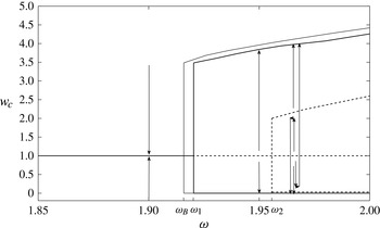
 ${\it\omega}_{1}<{\it\omega}<{\it\omega}_{2}$
) or oscillate around these centres due to a bifurcation of bounded instability modes (i.e. the breakdown states with
 ${\it\omega}>{\it\omega}_{2}$
). This indicates that the minimizer states are attraction points of flow dynamics, but that they may not necessarily be stable in response to small perturbations.
In § 3.7, we summarize the bifurcation diagram of solutions of the steady-state problem and the stability characteristics of each solution.
3.2. The steady-state problem
The dynamical problem defined by (2.1) and the assumed boundary conditions is well posed and, using relevant initial conditions for the stream function, circulation and azimuthal vorticity, describes the axisymmetric evolution of a swirling flow in a finite-length pipe. The columnar solid-body rotating flow, where
 $$\begin{eqnarray}{\it\psi}(x,y,t)=y,\quad K(x,y,t)=2{\it\omega}y,\quad {\it\chi}(x,y,t)=0,\end{eqnarray}$$
is a base steady-state solution of the problem for all time
 $t\geqslant 0$
and every level of
 ${\it\omega}$
. According to the linear stability analysis of Wang & Rusak (Reference Wang and Rusak1996a
,Reference Wang and Rusak
b
), this branch of states is asymptotically stable when
 $0\leqslant {\it\omega}<{\it\omega}_{1}$
, has a neutrally stable mode at
 ${\it\omega}={\it\omega}_{1}$
and is unstable when
 ${\it\omega}>{\it\omega}_{1}$
. Here,
 ${\it\omega}_{1}$
is the first critical swirl
 ${\it\omega}_{1}=\sqrt{{\it\omega}_{B}^{2}+{\rm\pi}^{2}/16L^{2}}$
, where
 ${\it\omega}_{B}=1.9159$
is Benjamin’s (Reference Benjamin1962) special swirl of a solid-body rotating flow. Moreover, the flow is unstable to instability modes that appear in sequence as swirl is increased above
 ${\it\omega}_{1}$
(see Gallaire, Chomaz & Huerre Reference Gallaire, Chomaz and Huerre2004). Therefore, a perturbed solid-body rotation flow with a swirl ratio above
 ${\it\omega}_{1}$
may evolve into other time-asymptotic (saturated) states. In this section, we seek to identify the bifurcation of additional steady states of the problem that may be time-asymptotic states of the flow dynamics. Using numerical simulations based on the system (2.1) with the assumed boundary conditions, we demonstrate in § 4 the dynamical connection and evolution of perturbed solid-body rotation states at
 ${\it\omega}>{\it\omega}_{1}$
to these additional states.
When the flow is steady, the circulation and the total head are conserved along a constant stream function and are therefore functions of
 ${\it\psi}$
only. Equations (2.1) can be then further reduced to a single partial differential equation (PDE) for the solution of the stream function
 ${\it\psi}$
, known as the Squire–Long equation (see Squire Reference Squire1960; Long Reference Long1953), hereafter abbreviated as SLE (also known as the Bragg & Hawthorne Reference Bragg and Hawthorne1950 equation), i.e.
 $$\begin{eqnarray}{\it\psi}_{yy}+\frac{{\it\psi}_{xx}}{2y}=H^{\prime }({\it\psi})-\frac{I^{\prime }({\it\psi})}{2y}.\end{eqnarray}$$
For an inlet solid-body rotating flow with a uniform axial velocity, where
 ${\it\psi}=y$
, the extended non-dimensional circulation function is
 $I({\it\psi})=2{\it\omega}^{2}{\it\psi}^{2}$
for
 $0\leqslant {\it\psi}\leqslant \frac{1}{2}$
. Also,
 $H$
is the non-dimensional total head function of the flow, defined as
 $H({\it\psi})=H_{0}+2{\it\omega}^{2}{\it\psi}$
for
 $0\leqslant {\it\psi}\leqslant \frac{1}{2}$
, where
 $H_{0}$
is the given total head at the pipe inlet centreline. In addition, to accommodate possible solutions with separation zones, we assume that
 $$\begin{eqnarray}I({\it\psi})=I(0)=0,\quad H({\it\psi})=H(0)=H_{0}\quad \text{and}\quad I^{\prime }({\it\psi})=H^{\prime }({\it\psi})=0\end{eqnarray}$$
when
 ${\it\psi}<0$
, and
 $$\begin{eqnarray}I({\it\psi})=I\left(\frac{1}{2}\right)=\frac{{\it\omega}^{2}}{2},\quad H({\it\psi})=H\left(\frac{1}{2}\right)=H_{0}+{\it\omega}^{2}\quad \text{and}\quad I^{\prime }({\it\psi})=H^{\prime }({\it\psi})=0\end{eqnarray}$$
when
 ${\it\psi}>\frac{1}{2}$
. This assumption extends the treatment of separation zones in Wang & Rusak (Reference Wang and Rusak1997) to include possible states with either centreline stagnation (breakdown) zones where
 ${\it\psi}=0$
or wall quasi-stagnation zones where
 ${\it\psi}=\frac{1}{2}$
. In the centreline stagnation zones, the three velocity components vanish. The inviscid flow simulations in § 4 show that the flow in these zones comes from an infinitesimally small incoming flux around the centreline that has no circulation and that extends to a finite-size zone with zero velocities. However, in the wall quasi-stagnation zones only the axial and radial velocity components vanish, while the circumferential velocity in these zones does not vanish and is
 $K(\frac{1}{2})/\sqrt{2y}$
. The inviscid flow simulations in § 4 show that the flow in the wall zones comes from an infinitesimally small incoming flux around the wall that has the wall circulation, and that this flow extends to a finite-size zone with zero axial and radial velocities, but with constant circulation. Under these assumptions, the SLE (3.2) becomes
 $$\begin{eqnarray}{\it\psi}_{yy}+\frac{{\it\psi}_{xx}}{2y}=2{\it\omega}^{2}\left(1-\frac{{\it\psi}}{y}\right)\quad \text{for}\ 0\leqslant {\it\psi}\leqslant \frac{1}{2}.\end{eqnarray}$$
The corresponding boundary conditions are as follows:
 $$\begin{eqnarray}\left.\begin{array}{@{}l@{}}{\it\psi}(0,y)=y\quad \text{and}\quad {\it\psi}_{x}(L,y)=0\quad \text{for}\ 0\leqslant y\leqslant {\textstyle \frac{1}{2}},\\ {\it\psi}(x,0)=0\quad \text{and}\quad {\it\psi}(x,{\textstyle \frac{1}{2}})={\textstyle \frac{1}{2}}\quad \text{for}\ 0\leqslant x\leqslant L.\end{array}\right\}\end{eqnarray}$$
The problem (3.5) and (3.6) with the extended definition of
 $I({\it\psi})$
and
 $H({\it\psi})$
according to (3.3) and (3.4) is linear when there is no separation zone and becomes nonlinear with the appearance of separation zones (a similar comment was also given by Leclaire & Sipp Reference Leclaire and Sipp2010). When either centreline or wall-separation zones appear, there is a need to determine the free separation surface. We note that Leclaire & Sipp (Reference Leclaire and Sipp2010) used a nonlinear analysis of the SLE to describe bifurcation diagrams that appear under two inlet conditions and found limit points for the first possible appearance of breakdown and wall-separation states.
3.3. Critical swirl levels and singular states
The solutions of the problem (3.5) and (3.6) with the same functions
 $H({\it\psi})$
and
 $I({\it\psi})$
are sought. For physical situations, we also look for solutions where no part of the outlet allows reverse flow, i.e.
 $0\leqslant {\it\psi}(x,y)\leqslant \frac{1}{2}$
in the whole flow domain
 $0\leqslant x\leqslant L$
and
 $0\leqslant y\leqslant \frac{1}{2}$
, and the outlet axial velocity is non-negative;
 ${\it\psi}_{y}(L,y)\geqslant 0$
for
 $0\leqslant y\leqslant \frac{1}{2}$
. A base solution of the problem for every swirl ratio
 ${\it\omega}\geqslant 0$
is the columnar state of a solid-body rotation flow with a constant axial velocity all along the pipe, where
 ${\it\psi}(x,y)=y$
,
 $I=2{\it\omega}^{2}y^{2}$
and
 $H=H_{0}+2{\it\omega}^{2}y$
. According to linear PDE theory, this is a unique classical solution of the problem for all swirl ratios
 ${\it\omega}\geqslant 0$
(without the use of stagnation zones), except for a sequence of critical swirl ratios
 ${\it\omega}_{(m,n)}$
(
 $m$
and
 $n$
are positive integers) where the linear PDE becomes singular. Only at these critical swirl ratios does a continuum of exact solutions of (3.5) and (3.6) exist, given by
 $$\begin{eqnarray}{\it\psi}_{(m,n)}(x,y;k)=y+k{\it\phi}_{m}(\,y)\sin \left(\frac{(2n-1){\rm\pi}x}{2L}\right),\end{eqnarray}$$
where
 $k$
is a constant. These states bifurcate at
 ${\it\omega}_{(m,n)}$
from the branch of columnar states (for which
 $k=0$
). The critical swirl ratios
 ${\it\omega}_{(m,n)}$
and the critical eigenmodes
 ${\it\phi}_{m}(\,y)$
are determined from the solution of the linear eigenvalue problem:
 $$\begin{eqnarray}\left.\begin{array}{@{}l@{}}\displaystyle {\it\phi}_{myy}+\left(4{\it\omega}_{(m,n)}^{2}-\frac{(2n-1)^{2}{\rm\pi}^{2}}{4L^{2}}\right)\frac{{\it\phi}_{m}}{2y}=0,\vspace{3.0pt}\\ {\it\phi}_{m}(0)={\it\phi}_{m}({\textstyle \frac{1}{2}})=0.\end{array}\right\}\end{eqnarray}$$
The solution of the problem (3.8) for all
 $m$
and
 $n$
shows that
 ${\it\omega}_{(m,n)}=\sqrt{{\it\omega}_{Bm}^{2}+(2n-1)^{2}{\rm\pi}^{2}/16L^{2}}$
and
 ${\it\phi}_{m}(\,y)=\sqrt{2y}\text{J}_{1}(2{\it\omega}_{Bm}\sqrt{2y})$
. Here,
 ${\it\omega}_{Bm}=j_{m}/2$
, where
 $j_{m}$
is the
 $m$
th zero of the Bessel function
 $\text{J}_{1}$
,
 $\text{J}_{1}(j_{m})=0$
. Note that
 ${\it\omega}_{B}={\it\omega}_{B1}=j_{1}/2=1.9159$
is Benjamin’s (Reference Benjamin1962) special swirl for the appearance of an infinitesimal long-wave perturbation on a solid-body rotation flow in an infinitely long pipe. In addition,
 ${\it\omega}_{B2}=j_{2}/2=3.5078$
and so on are higher-order special swirl levels according to Benjamin (Reference Benjamin1962). The resulting singular states at
 ${\it\omega}_{(m.n)}$
are given by
 $$\begin{eqnarray}{\it\psi}_{(m,n)}(x,y;k)=y+k\sqrt{2y}\text{J}_{1}\left(2{\it\omega}_{Bm}\sqrt{2y}\right)\sin \left(\frac{(2n-1){\rm\pi}x}{2L}\right)\end{eqnarray}$$
and the corresponding axial velocity is
 $$\begin{eqnarray}{\it\psi}_{(m,n)y}(x,y;k)=1+k\text{J}_{0}(2{\it\omega}_{Bm}\sqrt{2y})\sin ((2n-1){\rm\pi}x/2L).\end{eqnarray}$$
The range of the amplitude
 $k$
is determined for each
 $(m,n)$
by the requirement that
 $0\leqslant {\it\psi}(x,y)\leqslant \frac{1}{2}$
in the entire flow domain
 $0\leqslant x\leqslant L$
and
 $0\leqslant y\leqslant \frac{1}{2}$
.
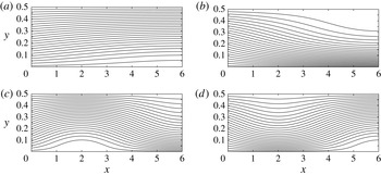
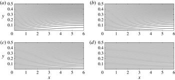
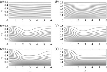
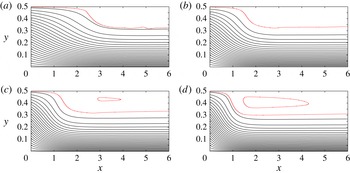
Singular limit states at
 ${\it\omega}_{1}=1.9203$
, (a) with
 $k=-1$
and (b) with
 $k=2.4829$
; and at
 ${\it\omega}_{2}=1.9557$
, (c) with
 $k=-1$
and (d) with
 $k=1$
.

In this paper, we focus on the flow behaviour in the range
 $0\leqslant {\it\omega}\leqslant 2$
, specifically when
 ${\it\omega}$
is between
 ${\it\omega}_{B}$
and 2, where the base flow changes its stability properties and additional steady-state solutions appear. For the case of
 $L=6$
, in this range of swirl there are two critical swirl levels, which are
 ${\it\omega}_{1}={\it\omega}_{(1,1)}=\sqrt{{\it\omega}_{B}^{2}+{\rm\pi}^{2}/16L^{2}}$
, the critical swirl of Wang & Rusak (Reference Wang and Rusak1996a
,Reference Wang and Rusak
b
) for a solid-body rotation flow in a finite-length pipe, and
 ${\it\omega}_{2}={\it\omega}_{(1,2)}=\sqrt{{\it\omega}_{B}^{2}+9{\rm\pi}^{2}/16L^{2}}$
, i.e.
 ${\it\omega}_{1}=1.9203$
and
 ${\it\omega}_{2}=1.9557$
. The higher-order critical states
 ${\it\omega}_{3}={\it\omega}_{(1,3)}=2.0246$
,
 ${\it\omega}_{4}={\it\omega}_{(1,4)}=2.1237$
and so on are beyond the scope of interest of this study. The singular states that appear at
 ${\it\omega}_{1}$
are given by
 ${\it\psi}_{(1,1)}(x,y;k)=y+k{\it\phi}_{B}(\,y)\sin ({\rm\pi}x/2L)$
where
 $-1\leqslant k\leqslant 1/(-\text{J}_{0}(j_{1}))$
. Here,
 ${\it\phi}_{B}(\,y)={\it\phi}_{1}(\,y)=\sqrt{2y}\text{J}_{1}(2{\it\omega}_{B}\sqrt{2y})$
is Benjamin’s (Reference Benjamin1962) first critical lateral mode. Since
 $j_{1}=3.8317$
and
 $\text{J}_{0}(j_{1})=-0.403$
,
 $k$
takes values in the range
 $-1\leqslant k\leqslant 2.4829$
. The limit states at
 $k=-1$
and
 $k=2.4829$
form two special states. A stagnation point appears at the pipe outlet centreline when
 $k=-1$
(see figure 1
a) and a stagnation point appears at the pipe outlet wall when
 $k=2.4829$
(see figure 1
b). The use of the stagnation zone assumption described above does not allow the singular solutions at
 ${\it\omega}_{1}$
to be continued beyond this range of
 $k$
. Instead, we find in § 3.5 that the branch of singular states at
 ${\it\omega}_{1}$
is connected at these two limit states to two branches of additional solutions with stagnation and quasi-stagnation zones when
 ${\it\omega}>{\it\omega}_{1}$
. We note that this first branch of bifurcating singular states at
 ${\it\omega}_{1}$
with the exact same limit states was first described in figures 11II.(a) and 14II.(c) of Leclaire & Sipp (Reference Leclaire and Sipp2010). These figures indicate the possible appearance of wall-separation zones in tandem with breakdown zones. We note that figures 11II.(b) and 14II.(b) of Leclaire & Sipp (Reference Leclaire and Sipp2010) also indicate the possible appearance of wall-separation zones at swirl levels below the first appearance of breakdown zones under the zero radial velocity inlet condition.
Similarly, the singular states that appear at
 ${\it\omega}_{2}$
are given by
 ${\it\psi}_{(1,2)}(x,y;k)=y+k{\it\phi}_{B}(\,y)\sin (3{\rm\pi}x/2L)$
, where
 $k$
is in the range
 $-1\leqslant k\leqslant 1$
. Again, the limit states at
 $k=-1$
and
 $k=1$
form two additional special states. A stagnation point appears along the pipe centreline at
 $x=L/3$
when
 $k=-1$
(see figure 1
c) and a stagnation point appears at the pipe outlet centreline when
 $k=1$
(see figure 1
d). As before, the use of the stagnation zone assumption does not allow the singular solutions at
 ${\it\omega}_{2}$
to be continued beyond this range of
 $k$
. Instead, the branch of singular states at
 ${\it\omega}_{2}$
is connected at these two limit states to two additional branches of solutions with stagnation zones when
 ${\it\omega}>{\it\omega}_{2}$
.
Using stability analysis techniques similar to the study by Wang & Rusak (Reference Wang and Rusak1996a
), it can be shown that all singular states that bifurcate at
 ${\it\omega}_{1}$
are neutrally stable and with no oscillations. The singular states that bifurcate at
 ${\it\omega}_{1}$
are built of an eigenfunction of the linearized SLE. Using these states as base states and applying an infinitesimally small unsteady perturbation again gives an eigenvalue problem for the perturbation growth rate that has a continuum of solutions with negative growth rates, expect for one mode that has the same shape function as the critical eigenfunction at
 ${\it\omega}_{1}$
, but with a zero growth rate. Therefore, all the singular states at
 ${\it\omega}_{1}$
are neutrally stable. These results can be deduced directly from Wang & Rusak (Reference Wang and Rusak1996b
) when analysis is applied to the case of a solid-body rotation.
The linear stability of the singular states that bifurcate at the higher-order critical swirls
 ${\it\omega}_{2},{\it\omega}_{3},\dots$
experience a similar situation as those at
 ${\it\omega}_{1}$
. However, since the base flow is already unstable at these critical states, and since the growth rate is a continuous function along the branch of solutions, these singular states must also have an unstable mode that is a solution of the linearized unsteady equation for these states as base flows.
The singular solutions described above are limited only to the critical states and do not yield stable saturated flow states at these swirl ratios, or at any other swirl ratio in between them. Therefore, a perturbed columnar state with swirl ratio at one of the critical swirls cannot stabilize on the columnar state or any of the singular states. Moreover, the continuation of the branch of singular states at
 ${\it\omega}_{1}$
to swirl levels above
 ${\it\omega}_{1}$
must include additional considerations.
3.4. Global analysis of the problem (3.5) and (3.6)
To extend the solutions manifold of the SLE (3.2), we use the variational principle associated with the SLE (3.2):
 $$\begin{eqnarray}\mathscr{E}({\it\psi};{\it\omega})=\int _{0}^{L}\int _{0}^{1/2}\left[\frac{{\it\psi}_{y}^{2}}{2}+\frac{{\it\psi}_{x}^{2}}{4y}+H({\it\psi})-\frac{I({\it\psi})}{2y}\right]\text{d}y\text{d}x.\end{eqnarray}$$
Here,
 $H({\it\psi})$
and
 $I({\it\psi})$
are defined above in their extended forms.
Following the global analysis of Wang & Rusak (Reference Wang and Rusak1997), the base flow state
 ${\it\psi}(\,y)=y$
is an asymptotically stable global minimizer state of the functional
 $\mathscr{E}({\it\psi};{\it\omega})$
when
 $0\leqslant {\it\omega}<{\it\omega}_{1}$
, it is a neutrally stable inflection state of
 $\mathscr{E}$
at
 ${\it\omega}={\it\omega}_{1}$
and it is an unstable min–max state of
 $\mathscr{E}({\it\psi};{\it\omega})$
when
 ${\it\omega}>{\it\omega}_{1}$
. In the swirl range
 ${\it\omega}>{\it\omega}_{1}$
, the unstable columnar flow must evolve in time. These facts formulate evidence that the corresponding functional value of
 $\mathscr{E}({\it\psi}(x,y,t);{\it\omega})$
decreases over sufficiently long time as the perturbed base flow evolves and thus
 ${\it\psi}(x,y,t)$
may asymptotically approach a minimizer state of
 $\mathscr{E}({\it\psi};{\it\omega})$
. Following Wang & Rusak (Reference Wang and Rusak1997), we can prove that under the following conditions:
-
(i)
 $H({\it\psi})$
and
$I({\it\psi})$
are bounded and piecewise-smooth, non-negative functions with bounded first derivatives; and
-
(ii)
$I({\it\psi})\leqslant c{\it\psi}^{q}$
where
$q$
is a fixed number,
$1<q\leqslant 2$
, and
$c>0$
;


the global minimizer state of
 $\mathscr{E}({\it\psi};{\it\omega})$
exists for every
 ${\it\omega}\geqslant 0$
. See details of the proof in Wang & Rusak (Reference Wang and Rusak1997, appendix A). Note that there exists a global minimizer state where
 $0\leqslant {\it\psi}(x,y)\leqslant \frac{1}{2}$
in the entire domain. Otherwise, assuming the global minimizer with
 $\bar{{\it\psi}}<0$
or
 $\bar{{\it\psi}}>\frac{1}{2}$
somewhere inside the domain, we may modify
 $\bar{{\it\psi}}$
to
 ${\it\psi}$
, defined by
 ${\it\psi}=0$
for every
 $(x,y)$
such that
 $\bar{{\it\psi}}(x,y)<0$
,
 ${\it\psi}=\frac{1}{2}$
for every
 $(x,y)$
such that
 $\bar{{\it\psi}}(x,y)>\frac{1}{2}$
and
 ${\it\psi}=\bar{{\it\psi}}$
elsewhere. One has
 $$\begin{eqnarray}\int _{0}^{L}\int _{0}^{1/2}\left[H(\bar{{\it\psi}})-\frac{I(\bar{{\it\psi}})}{2y}\right]\text{d}y\text{d}x=\int _{0}^{L}\int _{0}^{1/2}\left[H({\it\psi})-\frac{I({\it\psi})}{2y}\right]\text{d}y\text{d}x\end{eqnarray}$$
and
 $$\begin{eqnarray}\int _{0}^{L}\int _{0}^{1/2}\left[\frac{{\it\psi}_{y}^{2}}{2}+\frac{{\it\psi}_{x}^{2}}{4y}\right]\text{d}y\text{d}x\leqslant \int _{0}^{L}\int _{0}^{1/2}\left[\frac{\bar{{\it\psi}}_{y}^{2}}{2}+\frac{\bar{{\it\psi}}_{x}^{2}}{4y}\right]\text{d}y\text{d}x.\end{eqnarray}$$
Thus,
 $\mathscr{E}({\it\psi};{\it\omega})\leqslant \mathscr{E}(\bar{{\it\psi}};{\it\omega})$
and
 ${\it\psi}$
is a global minimizer itself. Actually,
 $\bar{{\it\psi}}={\it\psi}$
in the entire domain; otherwise, (3.12) is a strict inequality that contradicts the assumption that
 $\bar{{\it\psi}}$
is a minimizer. The global minimizer state represents a solution of the SLE (3.2) such that
 ${\it\psi}$
satisfies the SLE (3.2) wherever
 $0<{\it\psi}<\frac{1}{2}$
and
 ${\it\psi}(x,y)=0$
or
 ${\it\psi}=\frac{1}{2}$
elsewhere. Using similar analysis techniques, it can also be shown that a local minimizer state of
 $\mathscr{E}({\it\psi};{\it\omega})$
also exists for the case of a solid-body rotation flow when
 ${\it\omega}>{\it\omega}_{1}$
.
In a finite but long pipe setting
 $(L\gg 1)$
, Wang & Rusak (Reference Wang and Rusak1997, appendix B) showed that the steady global minimizer solution of
 $\mathscr{E}({\it\psi};{\it\omega})$
is comprised of two regions of flow development along the axial direction. There is a finite-length transition region from the given inlet state to a near-columnar state followed by a relatively long asymptotic axial decay region to an outlet columnar state
 ${\it\psi}(L,y)={\it\psi}_{c}(\,y)$
(the subscript
 $c$
is the notation for a columnar state) that is described by the solution of the columnar SLE problem
 $$\begin{eqnarray}{\it\psi}_{cyy}=2{\it\omega}^{2}\left(1-\frac{{\it\psi}_{c}}{y}\right)\quad \text{for}\ 0\leqslant {\it\psi}_{c}\leqslant \frac{1}{2},\end{eqnarray}$$
with conditions (3.3) and (3.4) and the boundary conditions
 $$\begin{eqnarray}{\it\psi}_{c}(0)=0\quad \text{and}\quad {\it\psi}_{c}({\textstyle \frac{1}{2}})={\textstyle \frac{1}{2}},\end{eqnarray}$$
and that is also a global minimum state of the corresponding columnar energy functional:
 $$\begin{eqnarray}E({\it\psi};{\it\omega})=\int _{0}^{1/2}\left[\frac{{\it\psi}_{y}^{2}}{2}+H({\it\psi})-\frac{I({\it\psi})}{2y}\right]\,\text{d}y.\end{eqnarray}$$
For a steady flow solution of the columnar (
 $x$
-independent) SLE problem,
 $E$
represents the flow force. Wang & Rusak (Reference Wang and Rusak1997) also showed that a steady-state solution of (3.2) with assumed boundary conditions must satisfy the following condition:
 $E({\it\psi}(0,y);{\it\omega})-E({\it\psi}(L,y);{\it\omega})\geqslant 0$
. Therefore, the physics of the global minimizer state of
 $\mathscr{E}({\it\psi};{\it\omega})$
may be interpreted in the following way: the swirling flow in a long but finite-length pipe tends to develop along the pipe into a columnar flow state with the minimum flow force at the pipe outlet that corresponds to the given
 ${\it\omega}$
. The applicability of this result to a finite-length pipe cannot be easily estimated theoretically but it can be tested via numerical simulations, by comparing the outlet states from the simulations with the theoretically predicted columnar minimizers. The agreement of the computed and predicted results presented in § 4 shows that in the present case, of an inlet solid-body rotation, a length of
 $L=6$
can be considered as sufficiently long. Similar comparisons also show that these properties apply to a local minimizer state of
 $\mathscr{E}({\it\psi};{\it\omega})$
, i.e. the local minimizer state develops along the pipe to an outlet state described by a local minimizer state of the columnar function
 $E({\it\psi};{\it\omega})$
.
We note that the solution of the variational problem for both the SLE (minimization of
 $\mathscr{E}({\it\psi};{\it\omega})$
) and the corresponding columnar SLE (minimization of
 $E({\it\psi};{\it\omega})$
) is a regular solution with a continuous gradient
 $\boldsymbol{{\rm\nabla}}{\it\psi}$
. Thus, the global minimizer state of
 $\mathscr{E}({\it\psi};{\it\omega})$
represents a flow field with a continuous velocity field. To illustrate the idea, we show the regularity of the solution of the variational problem for the columnar SLE. We assume that
 ${\it\psi}_{c}(\,y)$
is a minimizer of
 $E$
and that there is a corner point of
 ${\it\psi}_{c}(\,y)$
at some point
 $y=y_{0}\ (0<y_{0}<\frac{1}{2})$
such that
 ${\it\psi}_{c}(\,y)=0$
for
 $0\leqslant y\leqslant y_{0}$
and
 ${\it\psi}_{cy}(y_{0})>0$
. We choose a test function
 $\hat{{\it\psi}}_{c}(\,y)$
such that for a given
 ${\it\epsilon}>0$
,
 $\hat{{\it\psi}}_{c}(\,y)=(y-y_{0})+{\it\epsilon}$
for
 $y_{0}-{\it\epsilon}\leqslant y\leqslant y_{0}$
,
 $\hat{{\it\psi}}_{c}(\,y)=-(y-y_{0})+{\it\epsilon}$
for
 $y_{0}\leqslant y\leqslant y_{0}+{\it\epsilon}$
and
 $\hat{{\it\psi}}_{c}(\,y)=0$
elsewhere. We estimate the columnar functional increment
 $E({\it\psi}_{c}+\hat{{\it\psi}}_{c};{\it\omega})-E({\it\psi}_{c};{\it\omega})$
as follows:
 $$\begin{eqnarray}\displaystyle E({\it\psi}_{c}+\hat{{\it\psi}}_{c};{\it\omega})-E({\it\psi}_{c};{\it\omega}) & = & \displaystyle \int _{0}^{1/2}\left[\frac{({\it\psi}_{cy}+\hat{{\it\psi}}_{cy})^{2}}{2}+H({\it\psi}_{c}+\hat{{\it\psi}}_{c})-\frac{I({\it\psi}_{c}+\hat{{\it\psi}}_{c})}{2y}\right]\,\text{d}y\nonumber\\ \displaystyle & & \displaystyle -\,\int _{0}^{1/2}\left[\frac{({\it\psi}_{cy})^{2}}{2}+H({\it\psi}_{c})-\frac{I({\it\psi}_{c})}{2y}\right]\,\text{d}y\nonumber\\ \displaystyle & = & \displaystyle \int _{0}^{1/2}{\it\psi}_{cy}\hat{{\it\psi}}_{cy}\,\text{d}y+o({\it\epsilon})=-{\it\psi}_{cy}(y_{0}){\it\epsilon}+o({\it\epsilon}).\end{eqnarray}$$
Thus,
 $E({\it\psi}_{c}+\hat{{\it\psi}}_{c};{\it\omega})-E({\it\psi}_{c};{\it\omega})<0$
for sufficiently small
 ${\it\epsilon}$
. This contradicts the assumption that
 ${\it\psi}_{c}(\,y)$
is a minimizer solution of
 $E({\it\psi};{\it\omega})$
. The regularity of the minimizer state with a stagnation zone guarantees that the axial velocity at the zone interface is vanishing,
 ${\it\psi}_{cy}(y_{0})=0$
, that the pressure is the stagnation pressure, and that
 $H$
is continuous at the zone interface. Using similar arguments, it can be shown that the minimizer state with a quasi-stagnation zone is also a regular solution with no axial velocity along the zone interface and no jump of
 $H$
across the interface of the zone. Therefore, the minimizer solutions with a stagnation zone or with a quasi-stagnation zone are regular solutions of the Euler flow problem in the entire domain.
The above results simplify the analysis of solutions of the SLE (3.5) for the case of a long pipe. We look for solutions of the columnar (
 $x$
-independent) SLE problem given by the ordinary differential equation (ODE) for
 ${\it\psi}_{c}(\,y)$
. Global and local minimizer solutions of the columnar SLE problem (3.13) with (3.14) determine the outlet states of the global and local minimizer solutions of the SLE problem in a long pipe. Solutions of the columnar problem for
 ${\it\omega}>{\it\omega}_{1}$
may include states with either a stagnation zone around
 $y=0$
(where all velocity components vanish) or a quasi-stagnation zone attached to
 $y=\frac{1}{2}$
(where only the axial and radial velocity components vanish). The columnar SLE problem (3.13) and (3.14) is solved numerically using a fourth-order accurate Runge–Kutta integration scheme, where
 $Z_{1}={\it\psi}_{c}$
,
 $Z_{2}={\it\psi}_{cy}$
and then
 $Z_{1y}=Z_{2}$
,
 $Z_{2y}=2{\it\omega}^{2}(1-Z_{1}/y)$
for
 $0\leqslant y\leqslant \frac{1}{2}$
. The corresponding radial distribution of pressure
 $p_{c}(\,y)$
is determined from the steady radial momentum equation for a columnar flow:
 $$\begin{eqnarray}p_{cy}={\it\omega}^{2}\frac{{\it\psi}^{2}}{y^{2}}.\end{eqnarray}$$
The initial condition for solving the pressure according to (3.17) is determined from the solution type of the problem.
3.5. The uniqueness of the steady flow states when
$0\leqslant {\it\omega}<{\it\omega}_{1}$

We found in § 3.2 that multiple steady states coexist for inlet solid-body rotation flow when
 ${\it\omega}\geqslant {\it\omega}_{1}$
. Note that the original linear problem (3.2) only admits a unique solution for all non-critical swirl
 ${\it\omega}$
. The multiplicity of solutions of (3.5) results from the nonlinear nature of using the stagnation (or quasi-stagnation) model to represent the separation zone. It is important to know whether or not there exist multiple solutions of (3.5) for
 $0\leqslant {\it\omega}<{\it\omega}_{1}$
. For example, in the case of an inlet Lamb–Oseen vortex model, Wang & Rusak (Reference Wang and Rusak1997) showed that multiple solutions of the SLE exist when
 ${\it\omega}_{0}\leqslant {\it\omega}<{\it\omega}_{1}$
, where
 ${\it\omega}_{0}$
is another specific swirl level. A steady vortex-breakdown state can be established as a consequence of evolution of a perturbed columnar flow state within the swirl range
 ${\it\omega}_{0}\leqslant {\it\omega}<{\it\omega}_{1}$
. In this case, both the inlet flow and the outlet state are supercritical according to Wang & Rusak (Reference Wang and Rusak1997), i.e. the breakdown state is a supercritical–supercritical transition.
In contrast to the behaviour of the inlet Lamb–Oseen vortex, we show in this section that the columnar flow state is a unique solution of the SLE for an inlet solid-body rotation flow when
 $0\leqslant {\it\omega}<{\it\omega}_{1}$
, even though the problem is extended to include a stagnation zone. The direct consequence of this result is the non-existence of a steady breakdown state or a wall-separation state within the range
 $0\leqslant {\it\omega}<{\it\omega}_{1}$
. For such an inlet flow, we demonstrate in § 4, through numerical simulations, that the flow returns to a columnar state no matter how large the initial perturbation is. Breakdown and wall-separation states can only be established when the inlet flow is with
 ${\it\omega}>{\it\omega}_{1}$
. This shows that in the case of an inlet solid-body rotation flow, Benjamin’s supercritical–subcritical transition to describe vortex-breakdown states is not possible.
We start by giving a weak form of the solution of the SLE with a stagnation model through the variational principle (3.10). The variation
 ${\it\delta}\mathscr{E}({\it\psi})$
can be computed by the derivative
 $$\begin{eqnarray}\langle {\it\delta}\mathscr{E}({\it\psi}),\bar{{\it\psi}}\rangle =\left.\frac{\text{d}}{\text{d}{\it\epsilon}}\mathscr{E}({\it\psi}+{\it\epsilon}\bar{{\it\psi}})\right|_{{\it\epsilon}=0^{+}},\end{eqnarray}$$
where
 $\bar{{\it\psi}}$
is a test function that must satisfy the relevant homogeneous boundary conditions:
 $$\begin{eqnarray}\left.\begin{array}{@{}l@{}}\bar{{\it\psi}}(0,y)=0\quad \text{and}\quad \bar{{\it\psi}}_{x}(L,y)=0\quad \text{for}\ 0\leqslant y\leqslant {\textstyle \frac{1}{2}},\\ \bar{{\it\psi}}(x,0)=0\quad \text{and}\quad \bar{{\it\psi}}(x,{\textstyle \frac{1}{2}})=0\quad \text{for}\ 0\leqslant x\leqslant L.\end{array}\right\}\end{eqnarray}$$
It is clear that for a solution
 ${\it\psi}_{g}$
that is a minimizer state of
 $\mathscr{E}$
, we have
 $\langle {\it\delta}\mathscr{E}({\it\psi}_{g}),\bar{{\it\psi}}\rangle \geqslant 0$
for all test functions
 $\bar{{\it\psi}}$
.
We prove in appendix A the following useful result for the variation
 $\langle {\it\delta}\mathscr{E}({\it\psi}),\bar{{\it\psi}}\rangle$
about any state
 ${\it\psi}$
:
 $$\begin{eqnarray}\displaystyle \langle {\it\delta}\mathscr{E}({\it\psi}),\bar{{\it\psi}}\rangle & = & \displaystyle \int _{D}\left(\frac{{\it\psi}_{x}\bar{{\it\psi}}_{x}}{2y}+{\it\psi}_{y}\bar{{\it\psi}}_{y}\right)\text{d}x\text{d}y+2{\it\omega}^{2}\int _{D^{+}}\left(1-\frac{{\it\psi}}{y}\right)\bar{{\it\psi}}\text{d}x\text{d}y\nonumber\\ \displaystyle & & \displaystyle +\;2{\it\omega}^{2}\int _{D^{0}}\bar{{\it\psi}}^{+}\text{d}x\text{d}y-2{\it\omega}^{2}\int _{D^{1/2}}\left(y-\frac{1}{2}\right)\frac{\left(-\bar{{\it\psi}}\right)^{+}}{2y}\text{d}x\text{d}y,\end{eqnarray}$$
where
 $$\begin{eqnarray}(\bar{{\it\psi}})^{+}=\left\{\begin{array}{@{}ll@{}}\bar{{\it\psi}}\quad & \text{when}\ \bar{{\it\psi}}>0,\\ 0\quad & \text{when}\ \bar{{\it\psi}}\leqslant 0,\end{array}\right.\end{eqnarray}$$
and the various domains are
 $D=[0,L]\times [0,\frac{1}{2}]$
,
 $D^{+}=\{(x,y)\in D\text{ and }{\it\psi}(x,y)>0\}$
,
 $D^{0}=\{(x,y)\in D\text{ and }{\it\psi}(x,y)=0\}$
and
 $D^{1/2}=\{(x,y)\in D\text{ and }{\it\psi}(x,y)=\frac{1}{2}\}$
, respectively. Here,
 $D^{0}$
and
 $D^{1/2}$
represent the breakdown and wall-separation zones, respectively. The relationship
 $\langle {\it\delta}\mathscr{E}({\it\psi}),\bar{{\it\psi}}\rangle \geqslant 0$
for all test functions
 $\bar{{\it\psi}}$
is a definition of a solution
 ${\it\psi}$
of the SLE in the weak sense. In this way, the classical solution is extended to include solutions with a stagnation zone.
We first show that for an inlet solid-body rotation flow, the columnar flow is a unique minimizer state of the regular functional given by
 $$\begin{eqnarray}\tilde{\mathscr{E}}({\it\psi})=\int _{D}\left[\frac{{\it\psi}_{y}^{2}}{2}+\frac{{\it\psi}_{x}^{2}}{4y}+2{\it\omega}^{2}\left({\it\psi}-\frac{{\it\psi}^{2}}{2y}\right)\right]\text{d}y\text{d}x.\end{eqnarray}$$
Note that the critical swirl
 ${\it\omega}_{1}$
is determined by the Rayleigh quotient:
 $$\begin{eqnarray}2{\it\omega}_{1}^{2}=\min \frac{\displaystyle \int _{D}\left(\frac{\bar{{\it\psi}}_{x}^{2}}{2y}+\bar{{\it\psi}}_{y}^{2}\right)\text{d}y\text{d}x}{\displaystyle \int _{D}\frac{\bar{{\it\psi}}^{2}}{y}\text{d}y}\text{d}x.\end{eqnarray}$$
This is simply the variational formulation of the eigenvalue problem for the first critical flow state (see, e.g., Lieb & Loss Reference Lieb and Loss1997). In (3.23), the minimization is taken over all possible test functions
 $\bar{{\it\psi}}$
. From (3.23),
 $\tilde{\mathscr{E}}({\it\psi})$
is bounded from below when
 $0\leqslant {\it\omega}<{\it\omega}_{1}$
and thus a minimizer state of (3.22) is achieved using a standard compactness argument (see, e.g., Struwe Reference Struwe2008, p. 3). On the other hand, the columnar state
 ${\it\psi}=y$
is the sole regular solution of SLE and thus must be the sole minimizer state of the functional
 $\tilde{\mathscr{E}}({\it\psi})$
.
We show that there exists only a unique weak solution of (3.20), i.e.
 ${\it\psi}=y$
for
 $0\leqslant {\it\omega}<{\it\omega}_{1}$
. We assume that
 ${\it\psi}=y+\hat{{\it\psi}}$
is another possible solution of the problem and substitute it into (3.20):
 $$\begin{eqnarray}\displaystyle \langle {\it\delta}\mathscr{E}({\it\psi}),\bar{{\it\psi}}\rangle & = & \displaystyle \int _{D}\left(\frac{\hat{{\it\psi}}_{x}\bar{{\it\psi}}_{x}}{2y}+\hat{{\it\psi}}_{y}\bar{{\it\psi}}_{y}\right)\text{d}y\text{d}x-2{\it\omega}^{2}\int _{D^{+}}\frac{\hat{{\it\psi}}\bar{{\it\psi}}}{y}\text{d}y\text{d}x\nonumber\\ \displaystyle & & \displaystyle +\,2{\it\omega}^{2}\int _{D^{0}}\bar{{\it\psi}}^{+}\text{d}y\text{d}x-2{\it\omega}^{2}\int _{D^{1/2}}\left(y-\frac{1}{2}\right)\frac{\left(-\bar{{\it\psi}}\right)^{+}}{2y}\text{d}y\text{d}x.\end{eqnarray}$$
Let the test function
 $\bar{{\it\psi}}$
be
 $\bar{{\it\psi}}=-\hat{{\it\psi}}$
. Substituting this in (3.24), we obtain
 $$\begin{eqnarray}\displaystyle & & \displaystyle -\int _{D}\left(\frac{\hat{{\it\psi}}_{x}^{2}}{2y}+\hat{{\it\psi}}_{y}^{2}\right)\text{d}x\text{d}y+2{\it\omega}^{2}\int _{D^{+}}\frac{\hat{{\it\psi}}^{2}}{y}\text{d}x\text{d}y\nonumber\\ \displaystyle & & \displaystyle \quad +\,2{\it\omega}^{2}\int _{D^{0}}(-\hat{{\it\psi}})^{+}\text{d}x\text{d}y-2{\it\omega}^{2}\int _{D^{1/2}}\left(y-\frac{1}{2}\right)\frac{(\hat{{\it\psi}})^{+}}{2y}\text{d}y\text{d}x\geqslant 0.\end{eqnarray}$$
Using the fact that
 $\hat{{\it\psi}}=-y$
on
 $D^{0}$
and
 $\hat{{\it\psi}}=(\frac{1}{2}-y)^{+}$
on
 $D^{1/2}$
, and thus
 $\hat{{\it\psi}}^{2}/y=(-\bar{{\it\psi}})^{+}$
on
 $D^{0}$
and
 $D^{1/2}$
, we obtain
 $$\begin{eqnarray}\langle {\it\delta}\mathscr{E}({\it\psi}),-\hat{{\it\psi}}\rangle =-\int _{D}\left(\frac{\hat{{\it\psi}}_{x}^{2}}{2y}+\hat{{\it\psi}}_{y}^{2}\right)\text{d}x\text{d}y+2{\it\omega}^{2}\int _{D^{+}\cup D^{0}\cup D^{1/2}}\frac{\hat{{\it\psi}}^{2}}{y}\text{d}x\text{d}y\geqslant 0.\end{eqnarray}$$
Therefore, we must have
 $\hat{{\it\psi}}=0$
; otherwise, (3.26) contradicts (3.23) because
 ${\it\omega}<{\it\omega}_{1}$
and
 $$\begin{eqnarray}\int _{D^{+}\cup D^{0}\cup D^{1/2}}\frac{\hat{{\it\psi}}^{2}}{y}\text{d}x\text{d}y\leqslant 2{\it\omega}^{2}\int _{D}\frac{\hat{{\it\psi}}^{2}}{y}\text{d}x\text{d}y.\end{eqnarray}$$
This shows that the columnar solution
 ${\it\psi}=y$
is the only possible steady flow state when
 $0\leqslant {\it\omega}<{\it\omega}_{1}$
.
In a similar way, we can show that
 ${\it\psi}=y$
is the unique solution of the columnar SLE (3.13) when
 $0\leqslant {\it\omega}<{\it\omega}_{B}$
.
3.6. The bifurcation diagram of solutions of the columnar SLE problem
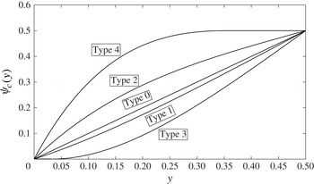
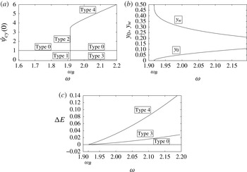
The columnar SLE problem (3.13) with (3.14) may have several solution types. The base type, denoted as type 0, is
 ${\it\psi}_{c}(\,y)=y$
, for which
 ${\it\psi}_{cy}(\,y)=1$
,
 $p_{c}(0)=1$
and
 $p_{c}(\,y)=1+{\it\omega}^{2}y$
. This solution is the base columnar state and exists for all
 ${\it\omega}$
. For this base state,
 $E({\it\psi}_{c};{\it\omega})=E_{0}({\it\omega})=1+{\it\omega}^{2}/8$
. An example of a type 0 solution is shown in figure 2 (here, the horizontal axis is
 $y$
in the range between 0 and
 $\frac{1}{2}$
and the vertical axis is
 ${\it\psi}_{c}(\,y)$
). As shown above, type 0 solutions are unique solutions of the columnar SLE problem when
 $0\leqslant {\it\omega}<{\it\omega}_{B}=1.9159$
. Also, type 0 solutions represent for all
 ${\it\omega}$
the outlet of the base columnar flow solutions of the SLE. These solutions are unique solutions of the SLE problem when
 ${\it\omega}<{\it\omega}_{1}$
.
Five types of solution of the columnar SLE problem (3.13) with (3.14). Type 0 is the base columnar flow solution for all
 ${\it\omega}$
. Type 1 is a solution with
 $0<{\it\psi}_{cy}(0)<1$
; the solution shown is for
 ${\it\omega}={\it\omega}_{B}$
, with
 $k=-0.25$
and
 ${\it\psi}_{cy}(0)=0.75$
. Type 2 is a solution with
 $1<{\it\psi}_{cy}(0)<3.4829$
; the solution shown is for
 ${\it\omega}={\it\omega}_{B}$
, with
 $k=1$
and
 ${\it\psi}_{cy}(0)=2$
. Type 3 is a solution with a centreline stagnation zone; the solution shown is for
 ${\it\omega}=1.95$
, with
 $y_{0}=0.0320$
. Type 4 is a solution with a wall quasi-stagnation zone; the solution shown is for
 ${\it\omega}=1.95$
, with
 $y_{w}=0.3515$
.

A branch of singular columnar states appears at Benjamin’s special swirl ratio
 ${\it\omega}={\it\omega}_{B}=1.9159$
, given by
 ${\it\psi}_{c}(\,y)=y+k\sqrt{2y}\text{J}_{1}(2{\it\omega}_{B}\sqrt{2y})$
, where
 $-1\leqslant k\leqslant 2.4829$
. When
 $-1\leqslant k<0$
, these solutions describe a decelerating flow near the centreline (
 $0<{\it\psi}_{cy}(0)<1$
) and an accelerating flow near the wall (
 $1<{\it\psi}_{cy}(\frac{1}{2})<1.4028$
), and are denoted as type 1 solutions. When
 $0<k<2.4829$
, these solutions describe an accelerating flow near the centreline (
 $1<{\it\psi}_{cy}(0)<3.4829$
) and a decelerating flow near the wall (
 $0\leqslant {\it\psi}_{cy}(\frac{1}{2})<1$
), and are denoted as type 2 solutions. Examples of type 1 and type 2 solutions at
 ${\it\omega}={\it\omega}_{B}$
for
 $k=-0.25$
and
 $k=1$
, respectively, are shown in figure 2. This set of solutions also represents singular columnar states in an infinitely long pipe at
 ${\it\omega}={\it\omega}_{B}$
. When
 $k=-1$
, a stagnation point occurs along the centreline; and when
 $k=2.4829$
, a stagnation point occurs at the pipe wall. The states with these special values of
 $k$
are bifurcation points for the appearance of additional types of solutions of the columnar SLE as
 ${\it\omega}$
increases above
 ${\it\omega}_{B}$
.
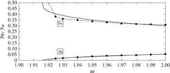
The type 3 solution is characterized by
 ${\it\psi}_{c}(\,y)={\it\psi}_{cy}(\,y)=0$
for
 $0\leqslant y\leqslant y_{0}$
, where
 $0<y_{0}<\frac{1}{2}$
is unknown and must be found as part of the solution iterations until convergence is achieved with the wall condition
 ${\it\psi}_{c}(\frac{1}{2})=\frac{1}{2}$
. The solution of the columnar SLE (3.13) with (3.14) is sought in the range
 $y_{0}\leqslant y\leqslant \frac{1}{2}$
, with conditions
 ${\it\psi}_{c}(y_{0})={\it\psi}_{cy}(y_{0})=0$
. In addition, from the Bernoulli law along the pipe centreline,
 $p_{c}(\,y)=\frac{3}{2}$
for the range
 $0\leqslant y\leqslant y_{0}$
and the initial condition for the pressure equation is
 $p_{c}(y_{0})=\frac{3}{2}$
. An example of a type 3 solution for the case of solid-body rotation at
 ${\it\omega}=1.95$
is also shown in figure 2. Type 3 solutions of the columnar SLE problem (3.13) and (3.14) represent a solution of the SLE problem (3.5) and (3.6) with an outlet that contains a finite-size stagnation zone around the centreline of radial width
 $\sqrt{2y_{0}}$
. These solutions correspond to steady vortex-breakdown states of the SLE problem (3.5) and (3.6).
The type 4 solution is characterized by
 ${\it\psi}_{c}(\,y)=\frac{1}{2}$
and
 ${\it\psi}_{cy}(\,y)=0$
for the range
 $y_{w}\leqslant y\leqslant \frac{1}{2}$
, where
 $0<y_{w}<\frac{1}{2}$
is unknown and must be found as part of the solution iterations. The solution of the columnar SLE is sought in the range
 $0\leqslant y\leqslant y_{w}$
, with conditions
 ${\it\psi}_{c}(y_{w})=\frac{1}{2}$
and
 ${\it\psi}_{cy}(y_{w})=0$
. In this case, the equation is integrated backwards from
 $y_{w}$
to 0, with repeated iteration until
 ${\it\psi}_{c}(0)=0$
is satisfied. It should be clarified that the axial and radial velocities are zero in the range
 $y_{w}\leqslant y\leqslant \frac{1}{2}$
. However, the circulation and the circumferential velocity do not vanish in this range. There,
 $K(\,y)={\it\omega}$
and
 $v(\,y)={\it\omega}/\sqrt{2y}$
. The pressure
 $p_{c}(y_{w})$
for a type 4 solution is determined in the following way. Along the pipe wall,
 $H(\frac{1}{2})=\frac{3}{2}+{\it\omega}^{2}$
and
 $K(\frac{1}{2})={\it\omega}$
. Then,
 $v(\frac{1}{2})={\it\omega}$
and from Bernoulli’s law along the streamline connecting the inlet wall to the outlet,
 $p_{c}(y_{w})=H(\frac{1}{2})-0.5K^{2}(\frac{1}{2})/2y_{w}=\frac{3}{2}+{\it\omega}^{2}-{\it\omega}^{2}/4y_{w}$
. An example of a type 4 solution for the case of solid-body rotation at
 ${\it\omega}=1.95$
is also shown in figure 2. The type 4 solutions of the columnar SLE problem (3.13) and (3.14) represent a solution of the SLE problem (3.5) and (3.6) with an outlet that contains a finite-size zero axial and radial velocity (quasi-stagnation) zone attached to the pipe wall. These solutions correspond to steady wall-separation states of the SLE problem (3.5) and (3.6).
The results of computations in the range
 $0\leqslant {\it\omega}\leqslant 2.2$
are summarized in the bifurcation diagram of solutions of the columnar SLE problem (see figure 3(a)). Here, the horizontal axis is the swirl ratio
 ${\it\omega}$
in the range
 $1.6\leqslant {\it\omega}\leqslant 2.2$
and the vertical axis is the value
 ${\it\psi}_{cy}(0)$
of each solution type. It can be seen that the columnar problem has a unique type 0 solution in the range
 $0\leqslant {\it\omega}<{\it\omega}_{B}=1.9159$
. At
 ${\it\omega}={\it\omega}_{B}=1.9159$
, there is a continuum of the singular columnar states of types 1 and 2. Three solutions may coexist when
 ${\it\omega}>{\it\omega}_{B}=1.9159$
, the base type 0 state and the type 3 and type 4 solutions. The type 3 and type 4 states start from the type 1 and type 2 special solutions at
 ${\it\omega}={\it\omega}_{B}$
with
 $k=-1$
and
 $k=2.4829$
, respectively. The corresponding sizes of
 $y_{0}$
(for type 3 solutions) and
 $y_{w}$
(for type 4 solutions) as a function of
 ${\it\omega}$
are shown in figure 3(b). It can be seen that
 $y_{0}$
increases from zero as
 ${\it\omega}$
increases above
 ${\it\omega}_{B}$
, while
 $y_{w}$
decreases from
 $\frac{1}{2}$
as
 ${\it\omega}$
increases above
 ${\it\omega}_{B}$
. These results indicate the increase in size of both the breakdown and the wall-separation zones with
 ${\it\omega}$
above
 ${\it\omega}_{B}$
.
Bifurcation diagrams of solutions of the columnar SLE problem (3.13) with (3.14) for the range of swirl ratio
 $1.6\leqslant {\it\omega}\leqslant 2.2$
. (a)
 ${\it\psi}_{cy}(0)$
of the various solution types as a function of
 ${\it\omega}$
; (b) separation zone sizes
 $y_{0}$
(for type 3 solutions) and
 $y_{w}$
(for type 4 solutions) as a function of
 ${\it\omega}$
; (c)
 ${\rm\Delta}E({\it\omega})=E_{0}({\it\omega})-E({\it\psi}_{c};{\it\omega})$
as a function of
 ${\it\omega}$
.

The computed values of
 ${\rm\Delta}E({\it\psi}_{c};{\it\omega})=E_{0}({\it\omega})-E({\it\psi}_{c};{\it\omega})$
for the various solution types are shown in figure 3(c). For the type 0 solutions,
 ${\rm\Delta}E({\it\psi}_{c};{\it\omega})=0$
for all
 ${\it\omega}$
. It can also be shown analytically that
 ${\rm\Delta}E({\it\psi}_{c};{\it\omega})=0$
for all the singular states at
 ${\it\omega}={\it\omega}_{B}=1.9159$
. Figure 3(c) shows
 ${\rm\Delta}E({\it\psi}_{c};{\it\omega})>0$
for both type 3 and type 4 solutions that appear when
 ${\it\omega}>{\it\omega}_{B}$
. Both solution types show that
 ${\rm\Delta}E({\it\psi}_{c};{\it\omega})$
increase with the increase of
 ${\it\omega}$
from
 ${\it\omega}_{B}$
. The type 4 solution exhibits a greater
 ${\rm\Delta}E({\it\psi}_{c};{\it\omega})$
than that of the type 3 solution. These results show that the base type 0 solution is a global minimum of
 $E$
when
 $0\leqslant {\it\omega}<{\it\omega}_{B}$
, an inflection point of
 $E$
when
 ${\it\omega}={\it\omega}_{B}$
and a min–max point of
 $E$
when
 ${\it\omega}>{\it\omega}_{B}$
. The type 3 and type 4 solutions of the columnar SLE are, respectively, local and global minimizer states of
 $E$
when
 ${\it\omega}>{\it\omega}_{B}$
.
3.7. Summary of solutions of the problem (3.2)–(3.4)
In § 3.5, we proved that the columnar flow state is a unique solution of the problem (3.2)–(3.4) when
 ${\it\omega}<{\it\omega}_{1}$
. The columnar flow solution is a global minimizer state of the functional
 $\mathscr{E}({\it\psi};{\it\omega})$
in this swirl range. The results of §§ 3.4 and 3.6 show that the columnar flow states are no longer global or a local minimizer states of
 $\mathscr{E}({\it\psi};{\it\omega})$
when
 ${\it\omega}>{\it\omega}_{1}$
. Based on the analysis of Wang & Rusak (Reference Wang and Rusak1997), the columnar flow state is actually an inflection state of
 $\mathscr{E}({\it\psi};{\it\omega})$
at
 ${\it\omega}={\it\omega}_{1}$
and a min–max state of
 $\mathscr{E}({\it\psi};{\it\omega})$
when
 ${\it\omega}>{\it\omega}_{1}$
.
In § 3.3, we find that a branch of singular states
 ${\it\psi}_{(1,1)}(x,y;k)$
with
 $-1\leqslant k\leqslant 2.4829$
appears at
 ${\it\omega}={\it\omega}_{1}$
and bifurcates from the branch of columnar flow states when
 $k$
approaches zero. There exist two limit states of this branch when
 $k=-1$
and
 $k=2.4829$
. The use of the stagnation zones assumption to represent separation zones does not allow continuation of the branch beyond this range of
 $k$
. In addition, since no solution other than the columnar state exists for
 ${\it\omega}<{\it\omega}_{1}$
, the branch of singular states at
 ${\it\omega}_{1}$
must continue by connecting at the two limit states with two branches of additional solutions of the problem when
 ${\it\omega}>{\it\omega}_{1}$
. Moreover, we find from §§ 3.4 and 3.6 that there exist branches of global and local minimizer states of the problem when
 ${\it\omega}>{\it\omega}_{1}$
. For a long pipe, these global and local minimizer states are dominated by an outlet flow that is given by the global and local minimizer solutions of the columnar SLE problem. The global minimizer states form a branch of wall-separation zones, while the local minimizer states form a branch of breakdown states. The branch of breakdown states starts at
 ${\it\omega}_{1}$
from the limit state
 ${\it\psi}_{(1,1)}$
with
 $k=-1$
, and the branch of wall-separation zones starts at
 ${\it\omega}_{1}$
from the state
 ${\it\psi}_{(1,1)}$
with
 $k=2.4829$
. Our numerical simulations, described in § 4, show that for these states the values of the axial velocity at the pipe outlet centreline as a function of
 ${\it\omega}>{\it\omega}_{1}$
are approximately given by the values
 ${\it\psi}_{cy}(0)$
of type 3 and type 4 solutions in figure 3(a). Our numerical flow simulations in § 4 show that the radial size of the breakdown zones as a function of
 ${\it\omega}>{\it\omega}_{1}$
is approximately given by
 $y_{0}$
in figure 3(b) and that the radial size of the wall-separation zones in this swirl range is approximately given by
 $y_{w}$
in figure 3(b). The longer the pipe is, the closer the agreement is with the columnar SLE results.
In § 3.3, we also find that a branch of singular states
 ${\it\psi}_{(1,2)}(x,y;k)$
with
 $-1\leqslant k\leqslant 1$
(see (3.9)) appears at
 ${\it\omega}={\it\omega}_{2}$
and also bifurcates from the branch of columnar flow states when
 $k$
approaches zero. These states do not have any counterpart solutions of the columnar SLE. Moreover, following Wang & Rusak (Reference Wang and Rusak1997), we can show that these states form a type of min–max state of
 $\mathscr{E}({\it\psi};{\it\omega})$
. Also, according to our flow simulations they do not represent any nonlinear saturated state of the flow dynamics. There are two limit states of this branch when
 $k=-1$
and
 $k=1$
. Again, the use of the stagnation zones assumption to represent separation zones does not allow continuation of the branch beyond this range of
 $k$
. From our numerical simulation, we do not find any evidence that there exist any states similar to the limit states when
 ${\it\omega}$
is near but below
 ${\it\omega}_{2}$
. Therefore, the branch of singular states at
 ${\it\omega}_{2}$
must continue by connecting the two limit states at
 $k=-1$
and
 $k=1$
with two additional branches of solutions of the problem for
 ${\it\omega}>{\it\omega}_{2}$
. Since there is no relationship between these states and the global and local minimizer solutions of the columnar SLE, these additional states must be additional min–max states of
 $\mathscr{E}({\it\psi};{\it\omega})$
. The existence of such min–max states may be proven by extending the analysis techniques of Wang & Rusak (Reference Wang and Rusak1997). It is expected that both branches of min–max states inherit the instability of the columnar states at
 ${\it\omega}>{\it\omega}_{2}$
, as well as the instability of the singular states at
 ${\it\omega}={\it\omega}_{2}$
and therefore are also unstable. Yet, our numerical flow simulations in § 4 demonstrate that these states form weak transient attractors of the flow dynamics where the flow passes near the min–max states, and then changes the evolution direction towards the global wall-separation or local breakdown minimizer states. A similar bifurcation of branches of min–max states with more wavy structures along the axial direction can be found from the limit points of the branches of singular states at
 ${\it\omega}_{3}$
,
 ${\it\omega}_{4}$
and so on. Such branches appear at
 ${\it\omega}>2$
when
 $L=6$
and are beyond the scope of this paper.
Bifurcation diagrams of solutions of the SLE problem (3.5) with boundary conditions (3.6) for the range of swirl ratio
 $1.85\leqslant {\it\omega}\leqslant 2$
. The heavy solid line represents stable columnar states, the dashed lines represent unstable states, the solid line with symbol
 $w$
represents numerically computed stable wall-separation states, the solid line with symbol
 $B$
represents numerically computed stable breakdown states, and the dotted line represents numerically computed breakdown states with bounded oscillations. The light line represents the bifurcation diagram of solutions of the columnar SLE problem from figure 3 and is shown for reference.

The results are summarized in the bifurcation diagram in figure 4 for a steady flow in a pipe with representative non-dimensional length
 $L=6$
in the range
 $0\leqslant {\it\omega}\leqslant 2$
. The horizontal axis is the swirl ratio
 ${\it\omega}$
of the inlet solid-body rotation. The vertical axis is a representative parameter of each solution given by
 $w_{c}$
. Here,
 $w_{c}$
equals the first maximum value of the centreline axial velocity
 $w(x,0)$
when the inlet slope
 $w_{x}(0,0)>0$
or the first minimum value of
 $w(x,0)$
when the inlet slope
 $w_{x}(0,0)<0$
. For the columnar states,
 $w_{c}=1$
for all
 ${\it\omega}$
. In the range
 $0\leqslant {\it\omega}\leqslant {\it\omega}_{1}$
, the columnar states are unique, stable and global minimizer states of
 $\mathscr{E}({\it\psi};{\it\omega})$
and are represented by the heavy solid line. In the range
 ${\it\omega}>{\it\omega}_{1}$
, the columnar states are unstable, min–max states
 $\mathscr{E}({\it\psi};{\it\omega})$
and are represented by a dashed line. At
 ${\it\omega}={\it\omega}_{1}=1.9203$
, there is a branch of singular neutrally stable states that bifurcates from the branch of columnar states and is represented by
 $w_{c}$
changing between 0 and 3.4829. Here,
 $w_{c}=w(L,0)$
for all singular states at
 ${\it\omega}_{1}$
. The limit states of this branch are represented by the points
 $({\it\omega}={\it\omega}_{1},w_{c}=0)$
and
 $({\it\omega}={\it\omega}_{1},w_{c}=3.4829)$
. A branch of breakdown states bifurcates from the first limit point towards the range
 ${\it\omega}>{\it\omega}_{1}$
and is represented by the heavy solid line with
 $w_{c}=0$
that starts from
 $({\it\omega}={\it\omega}_{1},w_{c}=0)$
. A branch of quasi-stagnant wall-separation zones bifurcates from the second limit point towards the range
 ${\it\omega}>{\it\omega}_{1}$
and is represented by the heavy solid line that starts from
 $({\it\omega}={\it\omega}_{1},w_{c}=3.4829)$
. At
 ${\it\omega}={\it\omega}_{2}=1.9557$
, there is a second branch of singular unstable states that bifurcates from the branch of columnar states and is represented by
 $w_{c}$
changing between 0 and 2. Here,
 $w_{c}=w(L/3,0)$
for all singular states at
 ${\it\omega}_{2}$
. The limit states of this branch are represented by the points
 $({\it\omega}={\it\omega}_{2},w_{c}=0)$
and
 $({\it\omega}={\it\omega}_{2},w_{c}=2)$
. A branch of min–max states of
 $\mathscr{E}({\it\psi};{\it\omega})$
bifurcates from the first limit point and is represented by the dashed line that starts from
 $({\it\omega}={\it\omega}_{2},w_{c}=0)$
. The states along this branch have a local stagnation zone around the centreline centred about
 $L/3$
and a small deceleration bubble near the wall outlet, and are similar to the state described in figure 1(c). Another branch of min–max states of
 $\mathscr{E}({\it\psi};{\it\omega})$
bifurcates from the second limit point and is represented by the dashed line that starts from
 $({\it\omega}={\it\omega}_{2},w_{c}=2)$
. The states along this branch have a local stagnation zone around the centreline outlet and a small deceleration bubble at the wall and around
 $x=L/3$
, and are similar to the state described in figure 1(d). In addition, we describe for reference the bifurcation diagram of solutions of the columnar SLE by the light solid lines. It can be seen that the bifurcation of states at
 ${\it\omega}_{1}$
is close to the bifurcation of solutions of the columnar problem. It is expected that the SLE solutions approach the columnar SLE solutions as
 $L$
increases.
We find from figure 4 that the columnar state is a unique state of the SLE problem when
 $0\leqslant {\it\omega}<{\it\omega}_{1}$
. The stability analysis of Wang & Rusak (Reference Wang and Rusak1996a
) showed that these states are asymptotically stable. There are three equilibrium states when
 ${\it\omega}_{1}<{\it\omega}<{\it\omega}_{2}$
: the columnar state, a breakdown state and a wall-separation state. The columnar state is unstable according to Wang & Rusak (Reference Wang and Rusak1996a
). From the numerical simulations in § 4, we infer that the breakdown and wall-separation states are stable centres of attraction of the flow dynamics. There are five equilibrium states when
 ${\it\omega}_{2}<{\it\omega}<{\it\omega}_{3}$
: the columnar state, two min–max states, a breakdown state and a wall-separation state. These columnar and min–max states are unstable according to Wang & Rusak (Reference Wang and Rusak1996a
) and Xu (Reference Xu2012). From the numerical simulations in § 4, we also infer that the wall-separation states are stable while the breakdown states experience bounded instabilities that bifurcate at
 ${\it\omega}_{2}$
. Similarly, additional states appear in sequence as the swirl ratio increases above higher-order critical states. This shows the complicated manifold of equilibrium states of the SLE as the inlet swirl ratio
 ${\it\omega}$
increases.
The bifurcation diagram in figure 4 also indicates for the expected dynamics of a perturbed solid-body rotation flow in a finite-length pipe. When
 $0\leqslant {\it\omega}<{\it\omega}_{1}$
, initial flow-accelerating or -decelerating perturbations, and even very large perturbations, decay in time and the flow returns to the asymptotically stable columnar state. This is indicated in figure 4 by the two arrows that point towards the columnar state at
 ${\it\omega}=1.9$
. When
 ${\it\omega}_{1}<{\it\omega}<{\it\omega}_{2}$
, initial decelerating perturbations will grow and stabilize on a breakdown state, while initial accelerating perturbations will grow and stabilize on the wall-separation state, with an equal chance of having evolution to either one of these states. This is indicated in figure 4 by the two arrows at
 ${\it\omega}=1.95$
that point from the columnar state towards the breakdown and wall-separation states. This is supported by the flow simulations in § 4. When
 ${\it\omega}_{2}<{\it\omega}<{\it\omega}_{3}$
, the initial perturbations may evolve in several ways. Large initial accelerating perturbations may grow, evolve away from the upper min–max state and be attracted to the wall-separation states. On the other hand, small initial accelerating perturbations may grow, be attracted to the upper min–max state, evolve near this state and then turn back and be attracted to a breakdown state. Similarly, large initial decelerating perturbations may grow, evolve away from the lower min–max state and be attracted to the breakdown state, while small initial decelerating perturbations may grow, be attracted to the lower min–max state, evolve near this state and then turn back and be attracted to a wall-separation state. This is indicated in figure 4 by the four arrows at
 ${\it\omega}=1.97$
that point from the columnar state towards the breakdown and wall-separation states. Again, there is an equal chance of having evolution to either one of these states. This demonstrates the possibly complicated dynamics of the flow, specifically as
 ${\it\omega}$
increases above
 ${\it\omega}_{2}$
and there are global and local minimizer states as well as min–max states that may affect the flow evolution. The numerical simulations reveal that the breakdown states experience the bifurcation of bounded instability waves when
 ${\it\omega}>{\it\omega}_{2}$
. We note that figure 4 provides an extension of the bifurcation diagrams presented in figures 11II.(a) and 14II.(a) of Leclaire & Sipp (Reference Leclaire and Sipp2010) under the zero azimuthal vorticity inlet condition studied in this paper.
4. Computed examples of flow dynamics
Numerical simulations that are based on the full system (2.1) (written in terms of
 $K$
and
 ${\it\eta}=\sqrt{2y}{\it\chi}$
) with the assumed boundary conditions are conducted. The flow simulation code uses a first-order accurate in time and second-order accurate in space explicit finite-difference scheme. It applies an upwind method in both the
 $x$
and
 $y$
directions in the estimation of the
 $x$
and
 $y$
derivatives of
 $K$
and
 ${\it\eta}$
. The upwind method uses a second-order backward-difference scheme when the local axial or radial velocity components are positive and a second-order forward-difference scheme when the local axial or radial velocity components are negative. A consistency analysis of the finite-difference equations shows that this numerical approach eliminates second derivatives in the numerical formulation. A second-order accurate Poisson solver for the spatial integration of
 ${\it\psi}$
in terms of
 ${\it\chi}$
is used. The method exhibits a low numerical viscosity (see Hoffman & Chiang Reference Hoffman and Chiang1993). However, an intermediate averaging of
 $K$
and
 ${\it\eta}$
is applied at every
 $I_{s}$
time steps (typically
 $I_{s}$
around 200) only when the perturbation becomes large and a near-stagnation (breakdown) or a quasi-stagnation (wall-separation) zone evolves in the flow. This averaging technique adds slight artificial viscosity to the numerical solution, diffuses localized, high-frequency numerical spike-like noise and small-scale vorticity packets within the low-speed separation zones and prevents it from growing. It has only a small, limited effect on the accuracy of computing the flow global dynamics shown below. We note that, with any given mesh, we use the maximum value of
 $I_{s}$
that leads the further growth of perturbations to either a breakdown zone or a wall-separation zone. Our numerical experience shows that
 $I_{smax}$
is proportional to the product of the discretization steps in space
 $({\rm\Delta}x)({\rm\Delta}y)$
when the time step
 ${\rm\Delta}t$
is fixed. In this way, the results of flow evolution converge with mesh refinement. For a detailed description of this numerical scheme and convergence studies with mesh refinement, see Granata (Reference Granata2014). It is also found that the computational method is stable when the Courant number is less than 0.2. A smaller time step
 ${\rm\Delta}t$
(with Courant number below 0.05) is typically used as the separation zones appear and evolve. This further increases the numerical accuracy of the integration in time. The method is stable and consistent with low numerical viscosity. This has been demonstrated in Rusak et al. (Reference Rusak, Wang, Xu and Taylor2012) through the agreement between the computed growth rate of small perturbations and the linear stability predictions according to the analysis of Wang & Rusak (Reference Wang and Rusak1996a
,Reference Wang and Rusak
b
). They also demonstrated an agreement of the nonlinear growth of perturbations with predictions according to their weakly nonlinear model. Such an agreement can be achieved only if the computational algorithm exhibits low numerical viscosity. All the computed results presented in this paper have also been tested for mesh convergence and show a similar agreement of growth rate of perturbations with the linear stability theory during the stage of linear growth of perturbations. Moreover, the computed time-asymptotic states of both the breakdown and the wall-separation states agree in their outlet shape with the solutions of the columnar SLE, providing additional confidence in the numerical simulations.
The computations demonstrate the evolution of flow dynamics and the existence of flows with both breakdown and wall-separation zones, depending on the initial perturbation on the solid-body rotation flow. We present snapshots of the instantaneous stream-function field
 ${\it\psi}(x,y,t)$
. We also describe the instantaneous change of the growth rate of the perturbation
 $\tilde{{\it\psi}}(x,y,t)$
with respect to the base columnar flow,
 $\tilde{{\it\psi}}(x,y,t)={\it\psi}(x,y,t)-y$
, which is defined as
 $$\begin{eqnarray}{\it\sigma}=\frac{1}{2}\frac{\text{d}}{\text{d}t}(\ln \Vert \tilde{{\it\psi}}(x,y,t)\Vert ^{2}).\end{eqnarray}$$
Here,
 $\Vert \tilde{{\it\psi}}(x,y,t)\Vert$
is the
 $L_{2}$
-norm of the perturbation
 $\tilde{{\it\psi}}(x,y,t)$
.
In all cases presented here, the initial perturbation for the numerical simulations is
 ${\it\psi}(x,y,0)=y+{\it\delta}{\it\phi}_{B}(\,y)\sin ({\rm\pi}x/2L)$
,
 ${\it\chi}(x,y,0)=-{\it\delta}[{\it\phi}_{Byy}(\,y)-({\rm\pi}/2L)^{2}{\it\phi}_{B}(\,y)/2y]$
 $\sin ({\rm\pi}x/2L)$
and
 $K(x,y,0)=2{\it\omega}y+2{\it\delta}{\it\omega}{\it\phi}_{B}(\,y)\sin ({\rm\pi}x/2L)$
. Here,
 ${\it\delta}$
is the size of the initial perturbation. The computed examples focus on the dynamics of the flow in a pipe of non-dimensional length
 $L=6$
at three representative swirl ratios
 ${\it\omega}=1.9$
,
 ${\it\omega}=1.95$
and
 ${\it\omega}=1.97$
around the first two critical swirls
 ${\it\omega}_{1}$
and
 ${\it\omega}_{2}$
. The results of the computed stream-function contours and of the rescaled instantaneous growth rate
 ${\it\sigma}^{\ast }={\it\sigma}L^{3}$
of the perturbation as a function of rescaled time
 $t^{\ast }=t/L^{3}$
are presented for all computations. We note that Grimshaw & Yi (Reference Grimshaw and Yi1993), Hanazaki (Reference Hanazaki1996) and Rusak et al. (Reference Rusak, Wang, Xu and Taylor2012) used this same rescaled time in their weakly nonlinear approaches. The present computed examples show that these rescaled parameters keep
 ${\it\sigma}^{\ast }$
and
 $t^{\ast }$
in a consistent order with the pipe length and with the near-critical swirl levels, and this results in numerical values of
 ${\it\sigma}^{\ast }$
and
 $t^{\ast }$
of the order
 $O(1)$
.
4.1. Case 1:
$0\leqslant {\it\omega}<{\it\omega}_{1}$

We first study an incoming solid-body rotation flow with a swirl ratio below the critical level,
 $0\leqslant {\it\omega}<{\it\omega}_{1}$
. We focus here on a representative case where
 ${\it\omega}$
is close to critical,
 ${\it\omega}=1.9<{\it\omega}_{1}=1.9203$
. Figure 5 describes the flow dynamics starting with a large initial perturbation
 ${\it\delta}=-1.111$
, where in the initial state there is a separation zone around the centreline and near the outlet (figure 5
a). Similarly, figure 6 describes the flow dynamics starting with a large initial perturbation
 ${\it\delta}=2.5$
, where in the initial state there is a separation zone attached to the pipe wall near the outlet (figure 6
a). The rescaled growth rates of the perturbations for both cases as a function of rescaled time
 $t^{\ast }$
are shown in figure 7 (the solid line is for the
 ${\it\delta}=-1.111$
case and the dashed line is for the
 ${\it\delta}=2.5$
case). The dotted line is the linear decay rate
 ${\it\sigma}^{\ast }=1.1005$
according to the analysis of Wang & Rusak (Reference Wang and Rusak1996a
,Reference Wang and Rusak
b
) for a solid-body rotation flow at
 ${\it\omega}=1.9$
in a finite-length pipe with
 $L=6$
. In both cases, after a short transition stage of decay of the higher-order modes during the time period
 $0<t^{\ast }<1$
, the perturbation forms the least stable linear mode of the flow at
 ${\it\omega}=1.9$
and decays in time (figure 5
b,c for the
 ${\it\delta}=-1.111$
case and figure 6
b,c for the
 ${\it\delta}=2.5$
case), with a constant linear decay rate
 ${\it\sigma}^{\ast }=-1.101$
. The flow returns to the columnar state when
 $t^{\ast }>2.78$
(figures 5
d and 6
d). These simulations are consistent with the result in § 3.5 that the columnar state at
 $0\leqslant {\it\omega}<{\it\omega}_{1}$
is a unique strong attractor of the flow dynamics with a wide basin of attraction, even when
 ${\it\omega}$
is close to
 ${\it\omega}_{1}$
and perturbations are large. Similar results are found for all swirl ratios
 $0\leqslant {\it\omega}<{\it\omega}_{1}$
. Also, this is clearly consistent with the result that, for an inlet flow with
 $0\leqslant {\it\omega}<{\it\omega}_{1}$
, the breakdown or wall-separation states do not exist, as proven above in § 3. The supercritical to subcritical jump transition according to Benjamin’s (Reference Benjamin1962) theory is not a possible scenario in this swirl range. The flow dynamics essentially follows a linear decay according to the least stable mode at the given
 ${\it\omega}<{\it\omega}_{1}$
, as predicted by the analysis given above and schematically described in figure 4 (by the arrows at
 ${\it\omega}=1.9$
).
Stream-function contour-line snapshots of flow evolution from a breakdown state to the columnar state when
 ${\it\omega}=1.9$
at (a)
 $t^{\ast }=0$
, (b)
 $t^{\ast }=0.463$
, (c)
 $t^{\ast }=1.157$
, (d)
 $t^{\ast }=2.315$
. The initial perturbation is with
 ${\it\delta}=-1.111$
. The flow runs from left to right: the left edge of the frame is the inlet, the right edge is the outlet, the bottom edge is the centreline
 ${\it\psi}=0$
and the upper edge is the pipe wall
 ${\it\psi}=0.5$
. There are 25 equi-spaced contour lines in each frame, ranging from 0.01 to 0.49.

Stream-function contour-line snapshots of flow evolution from a wall-separation state to the columnar state when
 ${\it\omega}=1.9$
at (a)
 $t^{\ast }=0$
, (b)
 $t^{\ast }=1.157$
, (c)
 $t^{\ast }=2.315$
and (d)
 $t^{\ast }=2.778$
. The initial perturbation is with
 ${\it\delta}=2.5$
. The flow runs from left to right: the left edge of each frame is the inlet, the right edge is the outlet, the bottom edge is the centreline
 ${\it\psi}=0$
and the upper edge is the pipe wall
 ${\it\psi}=0.5$
. There are 25 equi-spaced contour lines in each frame, ranging from 0.01 to 0.49.

The
 ${\it\sigma}^{\ast }$
of the decay of perturbations as a function of
 $t^{\ast }$
at
 ${\it\omega}=1.9$
: the solid line is for the case with
 ${\it\delta}=-1.111$
and the dashed line is for the case with
 ${\it\delta}=2.5$
. The dotted line is the linear stability decay rate at
 ${\it\omega}=1.9$
and with
 $L=6$
, as predicted by the analysis of Wang & Rusak (Reference Wang and Rusak1996a
).

4.2. Case 2:
${\it\omega}_{1}<{\it\omega}<{\it\omega}_{2}$

We now study the perturbed flow dynamics in the range
 ${\it\omega}_{1}<{\it\omega}<{\it\omega}_{2}$
. We focus on the representative case where
 ${\it\omega}=1.95>{\it\omega}_{1}=1.9203$
and
 ${\it\delta}=-0.111$
(figures 8 and 9). The flow stream-function contours in figure 8 show the growth of a small initial decelerating perturbation and the evolution to a breakdown state. The rescaled growth rate
 ${\it\sigma}^{\ast }$
of this process as a function of rescaled time
 $t^{\ast }$
is shown in figure 9(a). Also shown by the dotted line is the linear stability growth rate
 ${\it\sigma}^{\ast }=0.8143$
according to the analysis of Wang & Rusak (Reference Wang and Rusak1996a
,Reference Wang and Rusak
b
) for a solid-body rotation flow at
 ${\it\omega}=1.95$
in a finite-length pipe with
 $L=6$
. It can be seen that after a short transition stage of decay of the higher-order modes during
 $0<t^{\ast }<0.9$
, the growth of the perturbation is linear for the time period
 $0.9<t^{\ast }<2.7$
(figure 8
a,b), with a constant growth rate
 ${\it\sigma}^{\ast }=0.815$
. A stagnation point first appears along the centreline at
 $x=3$
when
 $t^{\ast }=2.96$
(figure 8
c). A near-stagnation zone develops around the centreline when
 $t^{\ast }>2.96$
, expands in both the radial and axial directions (figure 8
d,e), and evolves into a time-asymptotic state when
 $t^{\ast }>3.4$
. The flow state at
 $t^{\ast }=3.7$
(figure 8
f) is characterized by a large near-stagnation zone around the centreline, which resembles the local minimizer solution that was shown above to be the breakdown state in a long pipe. To demonstrate the correlation between the computed flow state at
 $t^{\ast }=3.7$
and the breakdown state according to the present theory, we describe in figure 9(b) a cross-section of
 ${\it\psi}(x=6,y,t^{\ast }=3.7)$
(the circles) and the solution of the columnar SLE for
 ${\it\omega}=1.95$
(the solid line in figure 9
b, taken from figure 2). The two solutions show agreement, specifically the appearance of a near-stagnation zone around the centreline. Similar results are found for all
 ${\it\omega}_{1}<{\it\omega}<{\it\omega}_{2}$
. This computation demonstrates that although the inlet flow in this case is above critical, the flow evolution is dominated by the linear process of Wang & Rusak (Reference Wang and Rusak1996a
,Reference Wang and Rusak
b
) instability and reaches a saturated nonlinear breakdown state, as predicted by the analysis developed in § 3 and described in figure 4 by the arrow pointing downwards at
 ${\it\omega}=1.95$
. This dynamical process to a saturated breakdown state is clearly not the scenario described by Benjamin’s vortex-breakdown theory, which allows only a supercritical to subcritical jump.
Stream-function contour-line snapshots of flow evolution from a near-columnar state to a breakdown state when
 ${\it\omega}=1.95$
at (a)
 $t^{\ast }=1.389$
, (b)
 $t^{\ast }=2.315$
, (c)
 $t^{\ast }=2.963$
, (d)
 $t^{\ast }=3.148$
, (e)
 $t^{\ast }=3.333$
and ( f)
 $t^{\ast }=3.704$
. The initial perturbation is with
 ${\it\delta}=-0.111$
. The flow runs from left to right: the left edge of each frame is the inlet, the right edge is the outlet, the bottom edge is the centreline
 ${\it\psi}=0$
and the upper edge is the pipe wall
 ${\it\psi}=0.5$
. There are 25 equi-spaced contour lines in each frame, ranging from 0.01 to 0.49.

The evolution of a perturbation with initial size
 ${\it\delta}=-0.111$
at
 ${\it\omega}=1.95$
. (a) The
 ${\it\sigma}^{\ast }$
value of the growth of the perturbation as a function of
 $t^{\ast }$
(solid line). The dotted line is the linear growth rate at
 ${\it\omega}=1.95$
and
 $L=6$
according to the analysis of Wang & Rusak (Reference Wang and Rusak1996a
,Reference Wang and Rusak
b
). (b) A comparison between the time-asymptotic outlet stream-function profile
 ${\it\psi}(x=L=6,y,t^{\ast }=3.704)$
of the breakdown state at
 ${\it\omega}=1.95$
(solid line) and the predicted outlet state
 ${\it\psi}_{c}(\,y)$
(type 3 solution from figure 2) at this swirl ratio (circles).

Figure 10 shows the results for the case where
 ${\it\omega}=1.95$
and
 ${\it\delta}=0.111$
. The flow stream-function contours show the growth of the small initial accelerating perturbation and the evolution to a wall-separation state. The rescaled growth rate
 ${\it\sigma}^{\ast }$
of this process as a function of
 $t^{\ast }$
is shown in figure 11(a). Also shown by the dotted line is the linear stability growth rate,
 ${\it\sigma}^{\ast }=0.8143$
, according to the analysis of Wang & Rusak (Reference Wang and Rusak1996a
,Reference Wang and Rusak
b
) for a solid-body rotation flow at
 ${\it\omega}=1.95$
and
 $L=6$
. It can be seen that after a short transition stage of decay of higher-order modes during
 $0<t^{\ast }<0.9$
, the growth of the perturbation is linear for the time period
 $0.9<t^{\ast }<3$
(figure 10
a,b) with a constant growth rate
 ${\it\sigma}^{\ast }=0.813$
. A stagnation point appears along the pipe wall at
 $x=3$
, when
 $t^{\ast }=3.89$
. A quasi-stagnation zone develops along the pipe wall (figure 10
c) when
 $t^{\ast }>3.89$
, expands in both the radial and axial directions (figure 10
d,e), and evolves into a time-asymptotic state when
 $t^{\ast }>4.6$
. The flow state at
 $t^{\ast }=4.72$
(figure 10
f) is characterized by a large quasi-stagnation zone attached to the wall, which resembles the solution that was shown above to be the wall-separation state in a long pipe. To demonstrate the correlation between the computed flow state at
 $t^{\ast }=4.72$
and the wall-separation state according to the present analysis, we present in figure 11(b) a cross-section of
 ${\it\psi}(x=6,y,t^{\ast }=4.72)$
(the circles) and the solution of the columnar SLE at
 ${\it\omega}=1.95$
(the solid line, taken from figure 2). The two solutions show agreement, specifically the appearance of a near-stagnation zone around the wall. This computation reveals the existence of a stable, wall-separation state in tandem with the breakdown state found in the previous computation, as predicted by the analysis developed in § 3 and described in figure 4 by the arrow pointing upwards at
 ${\it\omega}=1.95$
. The flow evolution is dominated by the linear process predicted by the analysis of Wang & Rusak (Reference Wang and Rusak1996a
,Reference Wang and Rusak
b
).
Stream-function contour-line snapshots of flow evolution from a near-columnar state to a wall-separation state when
 ${\it\omega}=1.95$
at (a)
 $t^{\ast }=1.389$
, (b)
 $t^{\ast }=2.778$
, (c)
 $t^{\ast }=4.167$
, (d)
 $t^{\ast }=4.398$
, (e)
 $t^{\ast }=4.514$
and ( f)
 $t^{\ast }=4.722$
. The initial perturbation is with
 ${\it\delta}=0.111$
. The flow runs from left to right: the left edge of each frame is the inlet, the right edge is the outlet, the bottom edge is the centreline
 ${\it\psi}=0$
and the upper edge is the pipe wall
 ${\it\psi}=0.5$
. There are 25 equi-spaced contour lines in each frame, ranging from 0.01 to 0.49.

The evolution of a perturbation with initial size
 ${\it\delta}=0.111$
at
 ${\it\omega}=1.95$
. (a) The
 ${\it\sigma}^{\ast }$
value of the growth of the perturbation as a function of
 $t^{\ast }$
(solid line). The dotted line is the linear growth rate at
 ${\it\omega}=1.95$
and
 $L=6$
according to the theory of Wang & Rusak (Reference Wang and Rusak1996a
,Reference Wang and Rusak
b
). (b) A comparison between the time-asymptotic outlet stream-function profile
 ${\it\psi}(x=L=6,y,t^{\ast }=4.722)$
of the wall-separation state at
 ${\it\omega}=1.95$
(solid line) and the predicted outlet state
 ${\it\psi}_{c}(\,y)$
(type 4 solution from figure 2) at this swirl ratio (circles).

Stream-function contour lines of time-asymptotic breakdown states at (a)
 ${\it\omega}=1.93$
, (b)
 ${\it\omega}=1.95$
, (c)
 ${\it\omega}=1.97$
and (d)
 ${\it\omega}=2$
. The flow runs from left to right: the left edge of each frame is the inlet, the right edge is the outlet, the bottom edge is the centreline
 ${\it\psi}=0$
and the upper edge is the pipe wall
 ${\it\psi}=0.5$
. There are 25 equi-spaced contour lines in each frame, ranging from 0.01 to 0.49. The dashed line is the
 ${\it\psi}=0.002$
contour and wraps around the breakdown zone.

Stream-function contour lines of time-asymptotic wall-separation states at (a)
 ${\it\omega}=1.93$
, (b)
 ${\it\omega}=1.95$
, (c)
 ${\it\omega}=1.97$
and (d)
 ${\it\omega}=2$
. The flow runs from left to right: the left edge of each frame is the inlet, the right edge is the outlet, the bottom edge is the centreline
 ${\it\psi}=0$
and the upper edge is the pipe wall
 ${\it\psi}=0.5$
. There are 25 equi-spaced contour lines in each frame, ranging from 0.01 to 0.49. The dashed line is the
 ${\it\psi}=0.496$
contour and wraps around the wall-separation zone.

4.3. A summary of the breakdown and wall-separation states in the range of swirl
$0\leqslant {\it\omega}<{\it\omega}_{3}$

We used the results of the breakdown and wall-separation states found at
 ${\it\omega}=1.95$
as initial states and slightly reduced the inlet swirl ratio, in small increments, to 1.94, 1.93 and 1.925. In each case, we allowed the flow to establish a time-asymptotic state. Similarly, we also progressively increased the swirl ratio to
 ${\it\omega}=1.96$
, 1.97, 1.98, 1.99 and
 ${\it\omega}=2$
. The time-asymptotic breakdown and wall-separation states at these swirl ratios are shown in figures 12 and 13, respectively. In each frame there are 25 equi-spaced contour lines, ranging from 0.01 to 0.49. The dashed line in figure 12(a–d) is the
 ${\it\psi}=0.002$
contour line that wraps around the breakdown zone. The dashed line is figure 13(a–d) is the
 ${\it\psi}=0.496$
contour line that wraps around the wall-separation zone. We note that some of the dashed lines are slightly wavy due to the limit of accuracy of the simulations in capturing such contour lines, which are close to either the centreline or the wall. It can be seen that both the breakdown zone and the wall-separation zone move upstream and increase in radial size as the swirl ratio increases from
 ${\it\omega}_{1}$
. In the range of swirl ratios studied here, the numerical simulations show that the wall-separation states appear to be asymptotically stable. However, while the breakdown states for
 ${\it\omega}_{1}=1.9203<{\it\omega}<{\it\omega}_{2}=1.9557$
also appear to be asymptotically stable, the numerical simulations show that the breakdown states at
 ${\it\omega}>{\it\omega}_{2}=1.9557$
are oscillating in time with a small amplitude and frequency that grow with the increase of
 ${\it\omega}$
above
 ${\it\omega}_{2}=1.9557$
. In addition, note that same nonlinear saturated and oscillating states are also found from perturbing the columnar states and allowing the flow to evolve for long time. Moreover, starting from either the breakdown or the wall-separation states at
 ${\it\omega}=1.925$
and reducing the swirl ratio to
 ${\it\omega}=1.92$
results in the decay of the perturbations over a long time back to the columnar state at
 ${\it\omega}=1.92$
. This indicates that
 ${\it\omega}_{1}$
is indeed a critical point of exchange of stability of the columnar flow states.
The correlation between the size of the breakdown and the wall-separation zones found from the simulations with the predicted size of these zones according to the columnar SLE problem is shown in figure 14. The value
 $y_{0}$
(the size of the breakdown zone) is determined from the simulations for each
 ${\it\omega}>{\it\omega}_{1}$
at the position
 $y$
at the pipe outlet where
 ${\it\psi}(L,y)=0.005$
. Similarly, the value
 $y_{w}$
(the size of the wall-separation zone) is determined from the simulations for each
 ${\it\omega}>{\it\omega}_{1}$
at the position
 $y$
at the pipe outlet where
 ${\it\psi}(L,y)=0.496$
. Figure 14 demonstrates an agreement between the computed time-asymptotic states and the prediction according to solutions of the columnar SLE for all
 ${\it\omega}>{\it\omega}_{1}$
, except very close to
 ${\it\omega}_{1}$
.
The size of
 $y_{0}$
and
 $y_{w}$
versus
 ${\it\omega}$
. The dashed lines with circles are computed results and the solid lines are the solutions of the columnar SLE.

Stream-function contour-line snapshots of flow evolution from a near-columnar state to a wall-separation state when
 ${\it\omega}=1.97$
at (a)
 $t^{\ast }=0$
, (b)
 $t^{\ast }=0.741$
, (c)
 $t^{\ast }=1.482$
, (d)
 $t^{\ast }=1.944$
, (e)
 $t^{\ast }=2.500$
and ( f)
 $t^{\ast }=3.519$
. The initial perturbation is with
 ${\it\delta}=-0.333$
. The flow runs from left to right: the left edge of each frame is the inlet, the right edge is the outlet, the bottom edge is the centreline
 ${\it\psi}=0$
and the upper edge is the pipe wall
 ${\it\psi}=0.5$
. There are 25 equi-spaced contour lines in each frame, ranging from 0.01 to 0.49.

Stream-function contour-line snapshots of flow evolution from a near-columnar state to a breakdown state when
 ${\it\omega}=1.97$
at (a)
 $t^{\ast }=0$
, (b)
 $t^{\ast }=0.741$
, (c)
 $t^{\ast }=1.574$
, (d)
 $t^{\ast }=2.315$
, (e)
 $t^{\ast }=3.241$
and ( f)
 $t^{\ast }=4.630$
. The initial perturbation is with
 ${\it\delta}=0.333$
. The flow runs from left to right: the left edge of each frame is the inlet, the right edge is the outlet, the bottom edge is the centreline
 ${\it\psi}=0$
and the upper edge is the pipe wall
 ${\it\psi}=0.5$
. There are 25 equi-spaced contour lines in each frame, ranging from 0.01 to 0.49.

4.4. Case 3:
${\it\omega}_{2}<{\it\omega}<{\it\omega}_{3}$

To complete the description of the dynamical behaviour of a perturbed solid-body rotation flow in the range
 ${\it\omega}_{2}<{\it\omega}<{\it\omega}_{3}$
, we study a representative case where
 ${\it\omega}=1.97$
and the initial perturbations are
 ${\it\delta}=-0.333$
and
 ${\it\delta}=0.333$
. Figure 15 describes snapshots of flow dynamics at
 ${\it\omega}=1.97$
when
 ${\it\delta}=-0.333$
. We can see that the initial decelerating perturbation (figure 15
a) grows in time (figure 15
b) and forms a stagnation point along the centreline at
 $x=2=L/3$
when
 $t^{\ast }=1.34$
. A small stagnation zone develops around
 $x=2$
and reaches a maximal radial size when
 $t^{\ast }=1.48$
, and at the same time a small deceleration zone appears near the outlet wall (figure 15
c). With further increase in time, the size of the breakdown zone actually decreases, while the size of the wall deceleration zone increases (figure 15
d at
 $t^{\ast }=1.94$
). We see that the flow dynamics is reversed at
 $t^{\ast }=1.48$
. This demonstrates that during the time period around
 $t^{\ast }=1.48$
, the flow passes close to a min–max stationary state that may be represented by the state in figure 15(c). Note that the state in figure 15(c) resembles the singular state found at
 ${\it\omega}={\it\omega}_{2}=1.9557$
with
 $k=-1$
(see figure 1
c) but the size of the perturbation is somewhat larger. This min–max state is a weak transient attractor of the flow dynamics during the time period
 $0.741<t^{\ast }<1.94$
. Note that the min–max state is an intermediate state between the breakdown state (shown in figure 16
e,f) and the wall-separation state (figure 15
f) at the swirl ratio
 ${\it\omega}=1.97$
. This reflects the nature of the mountain pass as it crosses the min–max solution. As the flow continues to evolve, a stagnation point develops at the wall outlet (figure 15
d at
 $t^{\ast }=1.94$
), followed by the establishment of a quasi-stagnation wall zone that moves upstream along the wall together with a significant flow acceleration along the centreline (figure 15
e at
 $t^{\ast }=2.5$
). When
 $t^{\ast }>3.33$
, the flow stabilizes on a saturation state that describes the same wall-separation state found above at
 ${\it\omega}=1.97$
(compare figure 15
f at
 $t^{\ast }=3.52$
with figure 13
c). A similar flow behaviour is found at all
 ${\it\omega}$
in the range between
 ${\it\omega}_{2}$
and
 ${\it\omega}_{3}$
.
The computed example in figure 15 shows that in the range
 ${\it\omega}_{2}<{\it\omega}<{\it\omega}_{3}$
, depending on the initial perturbations, the flow dynamics is strongly affected by the existence of the min–max state. Although the initial perturbation creates a deceleration along the pipe centreline and acceleration along the pipe wall, the min–max state forces a transient attraction during a period of the evolution and a reverse of flow dynamics to establish a wall-separation zone and flow acceleration along the pipe centreline. The min–max state is a crucial element in the understanding of this flow dynamics in the range
 ${\it\omega}_{2}<{\it\omega}<{\it\omega}_{3}$
, as described in figure 4 by the arrows that point to the wall-separation state at
 ${\it\omega}=1.97$
.
Figure 16 describes snapshots of flow dynamics at
 ${\it\omega}=1.97$
when now
 ${\it\delta}=0.333$
. We can see that the initial accelerating perturbation (figure 16
a) grows in time and forms along the pipe centreline a significant acceleration around
 $x=2=L/3$
and a deceleration near the outlet (figure 16
b). The perturbation continues to grow and reaches a maximal size of acceleration at
 $x=2$
and a stagnation point at the centreline outlet when
 $t^{\ast }=1.57$
(figure 16
c). With further increase in time, the flow acceleration around
 $x=2$
actually decreases, while the deceleration at the outlet stays nearly the same (figure 16
d at
 $t^{\ast }=2.31$
). We see that the flow dynamics is reversed at
 $t^{\ast }=1.57$
. This demonstrates that during the time period around
 $t^{\ast }=1.57$
, the flow passes close to another min–max stationary state that may be represented by the state in figure 16(c). Note that the state in figure 16(c) resembles the singular state found at
 ${\it\omega}={\it\omega}_{2}=1.9557$
with
 $k=1$
(see figure 1
d) but the size of the perturbation is somewhat larger. This min–max state is also a weak transient attractor of flow dynamics during the time period
 $0.740<t^{\ast }<2.31$
. As the flow continues to evolve, a near-stagnation zone develops at the outlet centreline with a significant flow acceleration along the wall (figure 16
e at
 $t^{\ast }=3.24$
). When
 $t^{\ast }>4.17$
, the flow stabilizes on the same breakdown state at
 ${\it\omega}=1.97$
with periodic convective waves inside it (figure 16
f at
 $t^{\ast }=4.63$
), as has been found in figure 12(c). A similar flow behaviour is found at all
 ${\it\omega}$
in the range between
 ${\it\omega}_{2}$
and
 ${\it\omega}_{3}$
.
The computed example in figure 16 shows that in the range
 ${\it\omega}_{2}<{\it\omega}<{\it\omega}_{3}$
, depending on the initial perturbations, the flow dynamics can also be strongly affected by the existence of the second min–max state at these swirl levels. Although the initial perturbation creates acceleration along the pipe centreline and deceleration along the pipe wall, the min–max state forces a transient attraction during a period of the evolution and a reverse of flow dynamics to establish a breakdown zone around the centreline and flow acceleration along the pipe wall. This second min–max state is also a crucial element in the understanding of the flow dynamics in the range
 ${\it\omega}_{2}<{\it\omega}<{\it\omega}_{3}$
, as described in figure 4 by the arrows that point to the breakdown state at
 ${\it\omega}=1.97$
.
5. Conclusions
The inviscid, incompressible and axisymmetric dynamics of perturbations on a solid-body rotation flow with a uniform axial velocity in a rotating, finite-length, straight and circular pipe with non-periodic inlet–outlet boundary conditions can be studied via global analysis methods and numerical simulations. We first analytically identify the critical swirl ratios
 ${\it\omega}_{1}$
,
 ${\it\omega}_{2}$
and so on where families of singular states appear. However, these branches of states are restricted by limit states and the continuation of the states along these branches requires a special analysis. We then define an energy functional
 $\mathscr{E}$
(given by (3.10)) that governs the inviscid and axisymmetric flow problem, and prove that there exist global and local minimizer states of this functional at every swirl ratio
 ${\it\omega}$
of the incoming flow. We show that the outlet state of the global and local minimizer states of
 $\mathscr{E}$
are described by solutions of the columnar SLE that are, respectively, global and local minimizer states of the columnar energy functional
 $E$
given by (3.15). We also prove that the base columnar flow state is a unique, global minimizer steady-state solution of the problem when the swirl level
 ${\it\omega}$
is below the first critical swirl ratio
 ${\it\omega}_{1}$
. However, when
 ${\it\omega}>{\it\omega}_{1}$
, the base columnar flow is an unstable min–max state of the energy functional
 $\mathscr{E}$
. We show that in addition to the base columnar flow state there exist states that describe swirling flows expanding around either axisymmetric centreline stagnant breakdown zones or axisymmetric wall quasi-stagnant zones where both axial and radial velocities vanish. These states are the local and the global minimizer states, respectively, of the energy functional
 $\mathscr{E}$
when
 ${\it\omega}>{\it\omega}_{1}$
. The size of these zones is approximately given by the solutions of the columnar SLE. We also claim the existence of min–max states when
 ${\it\omega}>{\it\omega}_{2}$
. We use these theoretical results to establish a global bifurcation diagram of steady-state solutions of the flow problem with an inlet solid-body rotation flow as a function of
 ${\it\omega}$
in the range
 $0\leqslant {\it\omega}<{\it\omega}_{3}$
.
The stability analysis of Wang & Rusak (Reference Wang and Rusak1996a
) shows that the columnar flow state is asymptotically stable and a global attractor of flow dynamics when
 $0\leqslant {\it\omega}<{\it\omega}_{1}$
. However, the columnar flow states are unstable when
 ${\it\omega}>{\it\omega}_{1}$
. The branch of singular states bifurcating at
 ${\it\omega}_{1}$
is composed of neutrally stable states, while the branches of singular states at the critical levels
 ${\it\omega}_{2}$
and above are also unstable states. Our numerical simulations show that the global (wall-separation) and local (breakdown) minimizer states of
 $\mathscr{E}$
that appear when
 ${\it\omega}>{\it\omega}_{1}$
are centres of attraction of the flow dynamics. We also infer from the numerical simulations that the wall-separation states are asymptotically stable when
 ${\it\omega}_{1}<{\it\omega}<{\it\omega}_{3}$
while the breakdown states are stable in the range
 ${\it\omega}_{1}<{\it\omega}<{\it\omega}_{2}$
and develop bounded oscillations when
 ${\it\omega}>{\it\omega}_{2}$
. The simulations also show that the min–max states that appear at
 ${\it\omega}>{\it\omega}_{2}$
are unstable but observed to be transient attractors of the flow dynamics.
The numerical simulations describe the evolution of perturbations on the above-critical columnar states to either the breakdown or the wall-separation states. The dynamics of growth of perturbations in both cases is composed of a linear stage of evolution, with growth rates predicted by the theory of Wang & Rusak (Reference Wang and Rusak1996a ), followed by a stage of attraction to either one of the separation states. The wall-separation states have the same chance of appearing as that of the vortex-breakdown states, and there is no hysteresis loop between them. This is strikingly different from the dynamics of vortices with a medium or narrow vortical core size. The present investigation establishes the existence of both wall-separation states in addition to vortex-breakdown zones at above-critical swirl levels and the dynamical path to these states as a function of initial perturbations. Through this study, the distinctive physics of a solid-body rotation flow with a uniform axial velocity entering a finite-length pipe is uncovered and understood at a fundamental mathematical level. This special behaviour was not carefully investigated in the previous experimental studies. The present paper provides the knowledge and insight to conduct further experimental investigations of solid-body rotation flows or large vortical core swirling flows in pipes. It also presents the foundation for generalization of results to three-dimensional flow states.
Appendix A
In this appendix, we derive an important formula for calculating the variation
 ${\it\delta}\mathscr{E}({\it\psi})$
of
 $\mathscr{E}$
around a certain state
 ${\it\psi}(x,y)$
, including a state that may contain a stagnation breakdown zone around the centreline or a quasi-stagnation wall-separation zone. Note that
 ${\it\psi}(x,y)$
is not necessarily a solution of the SLE. The variation
 ${\it\delta}\mathscr{E}({\it\psi})$
is defined by
 $$\begin{eqnarray}\langle {\it\delta}\mathscr{E}({\it\psi}),\bar{{\it\psi}}\rangle =\left.\frac{\text{d}}{\text{d}{\it\epsilon}}\mathscr{E}({\it\psi}+{\it\epsilon}\bar{{\it\psi}})\right|_{{\it\epsilon}=0^{+}},\end{eqnarray}$$
where
 $\bar{{\it\psi}}$
is a test function that must satisfy the relevant homogeneous boundary conditions. We prove the following theorem.
Theorem A.1.
 $$\begin{eqnarray}\displaystyle \langle {\it\delta}\mathscr{E}({\it\psi}),\bar{{\it\psi}}\rangle & = & \displaystyle \int _{D}\left(\frac{{\it\psi}_{x}\bar{{\it\psi}}_{x}}{2y}+{\it\psi}_{y}\bar{{\it\psi}}_{y}\right)\text{d}x\text{d}y+2{\it\omega}^{2}\int _{D^{+}}\left(1-\frac{{\it\psi}}{y}\right)\bar{{\it\psi}}\text{d}x\text{d}y\nonumber\\ \displaystyle & & \displaystyle +\,2{\it\omega}^{2}\int _{D^{0}}\bar{{\it\psi}}^{+}\text{d}x\text{d}y-2{\it\omega}^{2}\int _{D^{1/2}}\left(y-\frac{1}{2}\right)\frac{\left(-\bar{{\it\psi}}\right)^{+}}{2y}\text{d}x\text{d}y,\end{eqnarray}$$
where the various domains in (A 2) are
 $D=[0,L]\times [0,\frac{1}{2}]$
,
 $D^{+}=\{(x,y)\in D\text{ where }0<{\it\psi}(x,y)<\frac{1}{2}\}$
,
 $D^{0}=\{(x,y)\in D\text{ where }{\it\psi}(x,y)=0\}$
, and
 $D^{1/2}=\{(x,y)\in D\text{ where }{\it\psi}(x,y)=\frac{1}{2}\}$
, respectively.
Proof. We write
 $$\begin{eqnarray}\mathscr{E}(\bar{{\it\psi}})=\int _{D}\left[\frac{\bar{{\it\psi}}_{y}^{2}}{2}+\frac{\bar{{\it\psi}}_{x}^{2}}{4y}+2{\it\omega}^{2}\left((\bar{{\it\psi}})^{\odot }-\frac{(\bar{{\it\psi}})^{\odot 2}}{2y}\right)\right]\text{d}y\text{d}x,\end{eqnarray}$$
where
 $$\begin{eqnarray}(\bar{{\it\psi}})^{\odot }=\left\{\begin{array}{@{}ll@{}}{\textstyle \frac{1}{2}}\quad & \text{if }\bar{{\it\psi}}\geqslant {\textstyle \frac{1}{2}},\vspace{3.0pt}\\ \bar{{\it\psi}}\quad & \text{if }{\textstyle \frac{1}{2}}>\bar{{\it\psi}}>0,\vspace{3.0pt}\\ 0\quad & \text{if }\bar{{\it\psi}}\leqslant 0.\end{array}\right.\end{eqnarray}$$
We have
 $$\begin{eqnarray}\displaystyle \mathscr{E}({\it\psi}+{\it\epsilon}\bar{{\it\psi}}) & = & \displaystyle \int _{D}\left(\frac{({\it\psi}+{\it\epsilon}\bar{{\it\psi}})_{y}^{2}}{2}+\frac{({\it\psi}+{\it\epsilon}\bar{{\it\psi}})_{x}^{2}}{4y}\right)\text{d}y\text{d}x\nonumber\\ \displaystyle & & \displaystyle +\,2{\it\omega}^{2}\int _{D}\left(({\it\psi}+{\it\epsilon}\bar{{\it\psi}})^{\odot }-\frac{({\it\psi}+{\it\epsilon}\bar{{\it\psi}})^{\odot 2}}{2y}\right)\text{d}x\text{d}y.\end{eqnarray}$$
First, we find that
 $$\begin{eqnarray}\left.\frac{\text{d}}{\text{d}{\it\epsilon}}\left[\int _{D}\left(\frac{({\it\psi}+{\it\epsilon}\bar{{\it\psi}})_{y}^{2}}{2}+\frac{({\it\psi}+{\it\epsilon}\bar{{\it\psi}})_{x}^{2}}{4y}\right)\text{d}y\text{d}x\right]\right|_{{\it\epsilon}=0^{+}}=\int _{D}\left({\it\psi}_{y}\bar{{\it\psi}}_{y}+\frac{{\it\psi}\bar{{\it\psi}}_{x}}{2y}\right)\text{d}y\text{d}x.\end{eqnarray}$$
Next, we consider the derivative
 $$\begin{eqnarray}\left.\frac{\text{d}}{\text{d}{\it\epsilon}}\left(\int _{D}({\it\psi}+{\it\epsilon}\bar{{\it\psi}})^{\odot }\text{d}x\text{d}y\right)\right|_{{\it\epsilon}=0^{+}}=\lim _{{\it\epsilon}\rightarrow 0^{+}}\int _{D}\frac{({\it\psi}+{\it\epsilon}\bar{{\it\psi}})^{\odot }-({\it\psi})^{\odot }}{{\it\epsilon}}\text{d}x\text{d}y.\end{eqnarray}$$
In order to estimate (A 7), we also conduct a careful pointwise limit process and find that
 $$\begin{eqnarray}\lim _{{\it\epsilon}\rightarrow 0^{+}}\frac{({\it\psi}+{\it\epsilon}\bar{{\it\psi}})^{\odot }-({\it\psi})^{\odot }}{{\it\epsilon}}=\left\{\begin{array}{@{}ll@{}}\bar{{\it\psi}}(x,y)\quad & \text{if }(x,y)\in D^{+},\\ \bar{{\it\psi}}(x,y)^{+}\quad & \text{if }(x,y)\in D^{0},\\ -(-\bar{{\it\psi}}(x,y))^{+}\quad & \text{if }(x,y)\in D^{1/2},\\ 0\quad & \text{if either}\ {\it\psi}(x,y)<0\ \text{or}\ {\it\psi}(x,y)>{\textstyle \frac{1}{2}}.\end{array}\right.\end{eqnarray}$$
To be able to use (A 8) in (A 7), we need to pass the limit process into the integral. This requires that the integrand is controlled and is dominated by a certain integrable function. From the definition of
 $(\cdot )^{\odot }$
, we find that
 $$\begin{eqnarray}|(a)^{\odot }-(b)^{\odot }|<|a-b|\end{eqnarray}$$
and thus
 $$\begin{eqnarray}\left|\frac{({\it\psi}+{\it\epsilon}\bar{{\it\psi}})^{\odot }-({\it\psi})^{\odot }}{{\it\epsilon}}\right|\leqslant |\bar{{\it\psi}}|.\end{eqnarray}$$
By the Dominated Convergence Theorem (Lieb & Loss Reference Lieb and Loss1997), we obtain from (A 7)–(A 10)
 $$\begin{eqnarray}\left.\frac{\text{d}}{\text{d}{\it\epsilon}}\left(\int _{D}({\it\psi}+{\it\epsilon}\bar{{\it\psi}})^{\odot }\text{d}x\text{d}y\right)\right|_{{\it\epsilon}=0^{+}}=\int _{D^{+}}\bar{{\it\psi}}\text{d}x\text{d}y+\int _{D^{0}}\bar{{\it\psi}}^{+}\text{d}x\text{d}y-\int _{D^{1/2}}\left(\frac{1}{2}-\bar{{\it\psi}}\right)^{+}\text{d}x\text{d}y.\end{eqnarray}$$
In the same manner, we also obtain that
 $$\begin{eqnarray}\left.\frac{\text{d}}{\text{d}{\it\epsilon}}\left(\int _{D}\frac{({\it\psi}+{\it\epsilon}\bar{{\it\psi}})^{\odot 2}}{2y}\text{d}x\text{d}y\right)\right|_{{\it\epsilon}=0^{+}}=\int _{D^{+}}\frac{{\it\psi}\bar{{\it\psi}}}{y}\text{d}x\text{d}y-\int _{D^{1/2}}\frac{\left(-\bar{{\it\psi}}\right)^{+}}{2y}\text{d}x\text{d}y.\end{eqnarray}$$