1 Introduction
The dynamics of colloidal particles immersed in a fluid is moderated by the hydrodynamic interactions (HI) between the immersed bodies and driven in part by the fluctuating Brownian forces exerted on the particles due to collisions with individual solvent molecules, which are coupled to the HI through the fluctuation dissipation theorem (Kubo Reference Kubo1966). Fluid flows at the colloidal scale are dominated by viscous effects because the inertial relaxation time is much shorter than the viscous relaxation time, i.e. the Reynolds number is much less than one, so modelling dispersions via dynamic simulations requires generating efficient solutions to the Stokes equations subject to the no-slip boundary condition on the surfaces of all the immersed particles. A variety of methods, summarized in the next few paragraphs, have been developed for solving the Stokes equations around particles. These solution methods coupled with the Langevin equation, which describes the time evolution of particle positions, provide a sufficient description of particle motion to integrate particle coordinates in dynamic simulations.
The oldest and most established class of approximations applied to spherical particles are called implicit solvent methods. In these methods, the hydrodynamic mobility tensor, which is a linear transformation that describes how forces on one particle induce fluid flows that entrain another particle, is directly computed. The flow field produced by a given particle is approximated using the Green’s function for Stokes flow and a multipole expansion of the particle surface force density. In this way, the non-uniform hydrodynamic traction on each particle’s surface is represented as the sum of a force, torque, stresslet, etc., which sum together to propagate fluid flow (Kim & Karrila Reference Kim and Karrila2005). The motion of other particles entrained by this flow field is inferred via Faxén’s laws, which define how particles translate, rotate and deform in response to ambient flows.
In their seminal paper on Brownian dynamics (BD) simulations with HI, Ermak & McCammon (Reference Ermak and McCammon1978) used the Rotne–Prager–Yamawkawa (RPY) mobility (diffusion) tensor (Rotne & Prager Reference Rotne and Prager1969) to describe the coupling of particle motions in the underlying Langevin equation. The RPY tensor approximates the HI with the first-order terms in the multipole expansion of the force density on the surface of spherical particles (force monopole and isotropic quadrupole) summed pairwise over all particles. Three-body and higher-order multibody effects are neglected in the RPY tensor, but it is nevertheless an accurate description of the long-ranged coordination in colloidal dispersions. Higher-order approximations follow directly by extending the multipole expansion to arbitrary order. However, the hydrodynamic scattering series associated with the multipole expansion is slowly converging, especially for nearly touching particles, for which an infinite number of terms would be required to resolve the lubrication interactions (Ladd Reference Ladd1990). The Stokesian dynamics (SD) methodology (Brady & Bossis Reference Brady and Bossis1988) overcomes this problem by truncating the multipole expansion after the dipole (also retaining the isotropic components of the quadrupole and octupole), then closing the series with the exact expression for the hydrodynamic resistance between nearly touching particles (Jeffrey & Onishi Reference Jeffrey and Onishi1984; Jeffrey Reference Jeffrey1992b
). This scheme accurately reproduces the transport properties of colloidal dispersions across a wide range of volume fractions and Péclet numbers when lubrication flows dominate. For some transport properties, including sedimentation, higher-order multipoles may be necessary. Ladd (Reference Ladd1990) and Cichocki et al. (Reference Cichocki, Felderhof, Hinsen, Wajnryb and Bl/awzdziewicz1994) discuss approaches to account for these additional multipoles. The original implementation of the SD algorithm explicitly built the HI tensors, requiring
 $O(N^{2})$
calculations to build and
 $O(N^{3})$
to invert the matrices in a simulation of
 $N$
particles. The far-field HI stemming from the multipole expansion are slowly decaying and constitute the primary challenge in developing efficient simulation methods. The accelerated Stokesian dynamics (ASD) algorithm was developed by Sierou & Brady (Reference Sierou and Brady2001) address this problem. They applied the Ewald sum splitting of Hasimoto (Reference Hasimoto1959) and the particle-mesh-Ewald (PME) algorithm (Darden, York & Pedersen Reference Darden, York and Pedersen1993) to accelerate the far-field calculation, reducing the computational cost to
 $O(N\log N)$
. Wang & Brady (Reference Wang and Brady2016) later replaced the PME acceleration of the wave-space sum in ASD with spectral Ewald (SE) acceleration (Lindbo & Tornberg Reference Lindbo and Tornberg2010). The non-uniform fast Fourier transform (NUFFT) employed in the SE technique is spectrally accurate with independent and decoupled errors, and represents a substantial improvement in efficiency and error control over PME, although with no better asymptotic scaling.
Even with these accelerated techniques to compute the HI, the fluctuations associated with BD are challenging compute because they must be sampled from a distribution whose covariance is proportional to the hydrodynamic resistance tensor. This sampling requires computing the square root of the hydrodynamic resistance tensor, which is computationally expensive. In the original SD approach, direct Cholesky decomposition was used to compute the square root, requiring
 $O(N^{3})$
computations. Banchio & Brady (Reference Banchio and Brady2003) applied the Chebyshev polynomial approximation of Fixman (Reference Fixman1986) to compute the far-field Brownian forces, reducing the computational cost to
 $O(N^{1.25}\,\text{log}\,N)$
, which is still super-linear, limiting deployment in dynamic simulations to modest numbers of particles, typically
 $O(10^{2})$
. We recently published the positively split Ewald (PSE) method for rapidly sampling stochastic displacements in BD simulations with the RPY tensor, which evaluates the Brownian displacements with
 $O(N)$
computations (Fiore et al.
Reference Fiore, Usabiaga, Donev and Swan2017). We extended this method to the dipole level of the multipole expansion (Fiore & Swan Reference Fiore and Swan2018), which is equivalent to SD without lubrication. In this work, we develop a method incorporating the PSE sampling technique to achieve an
 $O(N)$
algorithm for SD with Brownian fluctuations.
In contrast to implicit solvent methods, explicit solvent techniques approximately solve the Navier–Stokes equations, rather than the Stokes equations, by representing the fluid as a collection of momentum conserving particles with prescribed rules for advection and collision with other fluid particles and with immersed colloidal particles. The lattice Boltzmann (Ladd, Colvin & Frenkel Reference Ladd, Colvin and Frenkel1988), dissipative particle dynamics (Hoogerbrugge & Koelman Reference Hoogerbrugge and Koelman1992) and multi-particle collision dynamics (Gompper et al.
Reference Gompper, Ihle, Kroll and Winkler2009) methods belong to this class of approximations. The overdamped behaviour characteristic of Stokes flow is then obtained by setting a suitably short time scale for vorticity diffusion and then integrating the fluid and particle dynamics on time scales that are short relative to the inertial relaxation time scale. Notably, Brownian forces are straightforward to include by introducing random forces on the fluid particles. Although these techniques nominally require
 $O(N)$
calculations per time step to simulate
 $N$
colloidal particles in a box of volume
 $L^{3}$
,
 $L^{2}/\unicode[STIX]{x1D708}\sim N^{2/3}$
time steps are required for vorticity to diffuse quickly throughout the system volume, where
 $\unicode[STIX]{x1D708}$
is the kinematic viscosity of the fluid, resulting in
 $O(N^{5/3})$
calculations if the vorticity diffusion rate is to be controlled at all length scales, as has been previously discussed (Fiore et al.
Reference Fiore, Usabiaga, Donev and Swan2017). To accurately model Stokes flow, for which vorticity diffusion is instantaneous, the algorithmic scaling of explicit solvent techniques is clearly undesirable. Furthermore, the true computational cost is actually
 $O(N+N_{s})$
, where
 $N_{s}$
is the total number of momentum-carrying solvent particles in the simulation volume. In many cases, particularly in dilute systems where more fluid particles are required to fill the void space between the immersed colloids,
 $N_{s}\gg N$
and the cost of evaluating the solvent-solving collisions can dominate the computational cost. Additionally, and importantly for the present work, the accuracy of the approximation used in these approaches is hard to systematically improve. For example it is clear that smaller fluid particles are required to more accurately resolve the flows between nearly touching particles and dense suspensions, but rigorous bounds on the error incurred by this approximation are challenging to impose.
Grid-based approaches such as the fluctuating immersed boundary method (FIB) (Delong et al. Reference Delong, Usabiaga, Delgado-Buscalioni, Griffith and Donev2014) and the force coupling method (FCM) (Lomholt & Maxey Reference Lomholt and Maxey2003; Keaveny Reference Keaveny2014; Delmotte & Keaveny Reference Delmotte and Keaveny2015) explicitly solve the continuum Stokes or Navier–Stokes equations throughout the simulation volume. These approaches use kernel, or envelope, functions to project particle forces onto a grid on which standard partial differential equation (PDE) solvers (finite difference, finite volume, spectral methods, etc.) can be used to compute the fluid response. Solving the Stokes equations in this way does not require the Green’s function, which is particularly advantageous for simulations with arbitrary boundaries. Adding Brownian forces is accomplished by introducing a fluctuating stress on the fluid grid. A shortcoming of these approaches is that, while the far-field hydrodynamic interaction is effectively RPY-like, the near-field or short-range hydrodynamic interactions depend on the specific kernel used to transfer data between the particles and the grid, and are therefore difficult to control independently. Yeo & Maxey (Reference Yeo and Maxey2010) showed how to incorporate more accurate expressions for the HI between nearly touching particles in the spirit of Stokesian dynamics, but it was unclear how these lubrication corrections could be combined with Brownian fluctuations in the context of that work.
Here we report the extension of the PSE method to include near-field lubrication corrections. This extension includes reformulating Stokesian dynamics itself as a saddle point problem, for which a highly effective constraint preconditioner is developed and applied. In this formulation, the Brownian stress is decomposed into a far-field Brownian slip velocity, computed using the PSE approach (Fiore & Swan Reference Fiore and Swan2018), and a near-field Brownian force, computed using a fast preconditioned Krylov subspace approximation (Chow & Saad Reference Chow and Saad2014). We show that this approach maintains the previously reported
 $O(N)$
scaling, and discuss algorithmic changes and optimization for graphics processing unit (GPU) implementation. This framework, while constructed for spherical particles, is generic and readily applied to many SD-like simulations of colloidal materials.
This paper is structured as follows. In § 2 we summarize Stokesian dynamics and present our reformulation of the equations for particle motion. In § 3 we discuss approximations for the hydrodynamic interactions between immersed particles. In § 4 we present fast methods to sample the near-field and far-field Brownian variables, as well as the Brownian drift. We describe the fast Stokesian dynamics (FSD) algorithm and give performance and validation results in § 5, with implementation details presented in appendix B. Finally, we present an application of the FSD method to simulations of particles with arbitrary shape in § 6, and discuss how to systematically improve the hydrodynamic approximation.
As the work in the following sections weaves together a number of existing results, extensions thereof and entirely new work into a cohesive framework, before commencing with the main discussion, it is worthwhile to pause and distinguish the upcoming information. The methods to be presented comprise five separate calculations:
(i) calculation of the far-field hydrodynamic interactions;
(ii) calculation of the near-field hydrodynamic interactions;
(iii) sampling of the stochastic far-field Brownian increments;
(iv) sampling of the stochastic near-field Brownian increments;
(v) solution of the hydrodynamic resistance problem coupling the far-field and near-field interactions.
The decision to decompose the hydrodynamic interactions into near-field and far-field contributions is based on the Stokesian dynamics approach (Brady & Bossis Reference Brady and Bossis1988). The far-field hydrodynamic interactions are computed using a mobility tensor constructed via multipole expansion, which is a well-known approach with an extensive history of use in the literature (see e.g. work by Rotne & Prager (Reference Rotne and Prager1969), Ladd (Reference Ladd1990), Cichocki et al. (Reference Cichocki, Felderhof, Hinsen, Wajnryb and Bl/awzdziewicz1994), Ichiki (Reference Ichiki2002), Kim & Karrila (Reference Kim and Karrila2005) and Fiore & Swan (Reference Fiore and Swan2018), among others). Although we will discuss the multipole expansion specifically, the framework developed herein admits use of other methods for computing the hydrodynamic mobility, e.g. the approaches developed by Delong et al. (Reference Delong, Usabiaga, Delgado-Buscalioni, Griffith and Donev2014) and Delmotte & Keaveny (Reference Delmotte and Keaveny2015).
Following the development of Stokesian dynamics and the ensuing improvements (Brady & Bossis Reference Brady and Bossis1988; Sierou & Brady Reference Sierou and Brady2001; Wang & Brady Reference Wang and Brady2016), the near-field hydrodynamic interactions are approximated using the exact two-body results of Jeffrey & Onishi (Reference Jeffrey and Onishi1984) and Jeffrey (Reference Jeffrey1992b ) modified to account for the interaction contribution already included in the far-field description. As with the far-field calculations, however, the framework presented here permits a wide range of near-field interaction descriptions.
Similar to the deterministic far-field interactions, the mobility perspective is used to compute the far-field contribution to the Brownian motion of the particles. Our previously published PSE method (Fiore et al. Reference Fiore, Usabiaga, Donev and Swan2017; Fiore & Swan Reference Fiore and Swan2018), which borrows ideas from fluctuating hydrodynamics (Delong et al. Reference Delong, Usabiaga, Delgado-Buscalioni, Griffith and Donev2014; Keaveny Reference Keaveny2014), is used to efficiently generate these stochastic velocities. The near-field contribution to Brownian is treated from the resistance perspective, resulting in stochastic forces which are sampled using a Krylov subspace method and a novel preconditioner. While the idea of accelerating stochastic sampling problems through preconditioning is not novel (see e.g. Chow & Saad Reference Chow and Saad2014), this particular approach and the preconditioners we present are new.
Finally, assembling the various far-field and near-field calculations into a cohesive framework for SD-like simulations that leverages the strengths of each approach is a challenge. Conventional SD approaches formulate the entire problem in the resistance perspective, requiring costly inversions of the far-field mobility (Brady & Bossis Reference Brady and Bossis1988; Sierou & Brady Reference Sierou and Brady2001; Wang & Brady Reference Wang and Brady2016). Furthermore, while fast approaches exist to compute the far-field increments in the form of velocities, conventional SD requires that these increments be in the form of forces (Banchio & Brady Reference Banchio and Brady2003). To solve the former issue, we cast the deterministic hydrodynamic problem as a saddle point matrix, unifying the far-field mobility and near-field resistance problems. Saddle point matrices find extensive use in science and engineering (Benzi, Golub & Liesen Reference Benzi, Golub and Liesen2005) and have been previously applied in the context of colloidal hydrodynamics for pure mobility problems (Balboa Usabiaga et al. Reference Balboa Usabiaga, Kallemov, Delmotte, Bhalla, Griffith and Donev2016; Sprinkle et al. Reference Sprinkle, Balboa Usabiaga, Patankar and Donev2017) and pure resistance problems (Meng & Higdon Reference Meng and Higdon2008a ), but have not been used before in mixed mobility and resistance formulations of colloidal hydrodynamics, as we do here. The Brownian sampling issue is addressed by computing a far-field slip velocity, as previously done by ourselves and others in the context of pure mobility problems (Delmotte & Keaveny Reference Delmotte and Keaveny2015; Balboa Usabiaga et al. Reference Balboa Usabiaga, Kallemov, Delmotte, Bhalla, Griffith and Donev2016; Sprinkle et al. Reference Sprinkle, Balboa Usabiaga, Patankar and Donev2017; Fiore & Swan Reference Fiore and Swan2018). This is the first application of this technique to Stokesian dynamics, where it is enables a mixed mobility–resistance formulation of the hydrodynamic interactions. The new methods we have developed and the particular combination of existing techniques with which we have integrated them collectively represent a formulation for Stokesian dynamics with Brownian motion that for the first time maintains an overall linear scaling in computational complexity with respect to the number of particles modelled.
2 Stokesian dynamics
As particles move through a viscous fluid, they propagate flows that entrain other particles. Hydrodynamic forces couple together the trajectories of these particles, creating a complex dynamical scenario. At the colloidal scale, inertia can be neglected and these flows are governed by the Stokes equations. In an infinite, dilute dispersion, the strength of these disturbance flows decays to leading order with the inverse of the distance from the particle that propagated the flow. The flow propagated by the whole dispersion is in principle divergent, but can be regularized by considering principles of mass conservation within the whole fluid–solid system. A consequence of this regularization is that the motion of all the particles in the dispersion is coupled. The coupling is linear because the Stokes equations are linear, and is described using either the mobility tensor
 $\unicode[STIX]{x1D648}_{UF}$
, which maps the hydrodynamic forces on particles
 $\boldsymbol{F}^{H}$
to the resulting velocity
 $\boldsymbol{U}=-\unicode[STIX]{x1D648}_{UF}\boldsymbol{\cdot }\boldsymbol{F}^{H}$
, or its inverse, the resistance tensor
 $\unicode[STIX]{x1D64D}_{FU}=\unicode[STIX]{x1D648}_{UF}^{-1}$
, which maps particle velocities to the resulting hydrodynamic drag force
 $\boldsymbol{F}^{H}=-\unicode[STIX]{x1D64D}_{FU}\boldsymbol{\cdot }\boldsymbol{U}$
. The discrete particle displacement equation used for our dynamic simulations is
 $$\begin{eqnarray}\boldsymbol{U}-\boldsymbol{U}^{\infty }=\unicode[STIX]{x1D64D}_{FU}^{-1}\boldsymbol{\cdot }(\boldsymbol{F}^{P}+\unicode[STIX]{x1D64D}_{FE}\boldsymbol{ : }\boldsymbol{E}^{\infty })+\boldsymbol{F}^{B}+k_{B}T\unicode[STIX]{x1D735}\boldsymbol{\cdot }\unicode[STIX]{x1D64D}_{FU}^{-1},\end{eqnarray}$$
which can be derived as the linearly accurate solution to the inertial
 $N$
-body Langevin equation in the over-damped limit (Hinch Reference Hinch1975; Roux Reference Roux1992). In (2.1),
 $\boldsymbol{U}=\unicode[STIX]{x0394}\boldsymbol{x}/\unicode[STIX]{x0394}t$
is the set of particle velocities, where
 $\unicode[STIX]{x0394}\boldsymbol{x}$
is the set of particle displacements over the discrete time step
 $\unicode[STIX]{x0394}t$
,
 $\boldsymbol{F}^{H}$
is the hydrodynamic force experienced by the particles,
 $\boldsymbol{F}^{B}$
is the stochastic Brownian force, given by
 $\sqrt{2k_{B}T/\unicode[STIX]{x0394}t}\,\unicode[STIX]{x1D64D}_{FU}^{1/2}\boldsymbol{\cdot }\unicode[STIX]{x1D733}$
in accordance with the fluctuation–dissipation theorem, where
 $\unicode[STIX]{x1D733}$
is a vector of independent standard Gaussian random variables, and
 $\boldsymbol{F}^{P}$
is the set of forces applied on particles due to e.g. external fields or interparticle potentials. Here, we consider the possibility of a linear background flow field characterized by position-dependent velocity
 $\boldsymbol{U}^{\infty }$
and constant rate of strain
 $\boldsymbol{E}^{\infty }$
. The right-hand side of (2.1) evaluates the translational and rotational velocities of the particles relative to the background flow. The quantity
 $\unicode[STIX]{x1D64D}_{FE}\boldsymbol{ : }\boldsymbol{E}^{\infty }$
is the additional hydrodynamic force experienced by the particles due to the imposed flow. The last term,
 $\unicode[STIX]{x1D735}\boldsymbol{\cdot }\unicode[STIX]{x1D64D}_{FU}^{-1}$
is commonly called the Brownian drift. Physically, it serves as an additional flux that drives particles away from low mobility configurations, ensuring they do not accumulate there. Its presence is required to ensure stationarity under the Gibbs–Boltzmann distribution and generate particle configurations with the correct statistics at equilibrium. We have previously shown that neglecting the drift introduces spurious long-range fluctuations in particle density, observed as a depression in the structure factor at small wavenumbers for non-interacting particles and an enhancement in the small wavenumber structure factor for hard sphere particles (Fiore & Swan Reference Fiore and Swan2018).
With a suitable approximation for
 $\unicode[STIX]{x1D64D}_{FU}$
and
 $\unicode[STIX]{x1D64D}_{FE}$
, equation (2.1) specifies the velocity of a collection of particles used to integrate particle trajectories in dynamic simulations of colloidal dispersions. In Stokesian dynamics,
 $\unicode[STIX]{x1D64D}_{FU}$
is constructed by combining a far-field approximation for the mobility
 ${\mathcal{M}}$
, which is accurate for relatively large interparticle separations, with specific near-field expressions for the interactions between nearly touching particles
 $\unicode[STIX]{x1D64D}_{FU}^{nf}$
,
 $$\begin{eqnarray}\unicode[STIX]{x1D64D}_{FU}={\mathcal{B}}^{\text{T}}\boldsymbol{\cdot }{\mathcal{M}}^{-1}\boldsymbol{\cdot }{\mathcal{B}}+\unicode[STIX]{x1D64D}_{FU}^{nf}.\end{eqnarray}$$
For rigid particles, the matrix
 ${\mathcal{B}}$
maps the allowable set of particle motions, e.g. translation and rotation, onto the (potentially) higher-order set of local motions and deformations described in the mobility coupling
 ${\mathcal{M}}$
, and its adjoint
 ${\mathcal{B}}^{\text{T}}$
projects the forces associated with the allowed motions, e.g. linear force and torque, out of the general moments of the hydrodynamic force density (traction) considered in
 ${\mathcal{M}}$
. Examples of the projections due to
 ${\mathcal{B}}$
and
 ${\mathcal{B}}^{\text{T}}$
are as follows:
 $$\begin{eqnarray}\left[\begin{array}{@{}c@{}}\boldsymbol{U}\\ \mathbf{0}\end{array}\right]={\mathcal{B}}\boldsymbol{\cdot }\boldsymbol{U},\quad \boldsymbol{F}={\mathcal{B}}^{\text{T}}\boldsymbol{\cdot }\left[\begin{array}{@{}c@{}}\boldsymbol{F}\\ \boldsymbol{ S}\end{array}\right].\end{eqnarray}$$
In the traditional SD formulation,
 ${\mathcal{M}}$
is constructed from the multipole expansion of the particle surface force density truncated after the dipole, and
 $\unicode[STIX]{x1D64D}^{nf}$
is built pairwise from analytical results developed by Jeffrey & Onishi (Reference Jeffrey and Onishi1984) for the lubrication interactions between a pair of particles less a far-field corrective term (Brady & Bossis Reference Brady and Bossis1988). In this case,
 ${\mathcal{B}}$
corresponds to the stresslet constraint,
 $$\begin{eqnarray}{\mathcal{M}}\boldsymbol{\cdot }{\mathcal{F}}+{\mathcal{B}}\boldsymbol{\cdot }\boldsymbol{U}=\mathbf{0},\end{eqnarray}$$
where
 ${\mathcal{F}}$
is the set of hydrodynamic force moments, including the force, torque and stresslet, as we have discussed previously (Fiore & Swan Reference Fiore and Swan2018). However, equation (2.2) is not limited to these approximations. The far-field multipole expansion could be truncated earlier, after the monopole and irreducible quadrupole, producing Rotne–Prager interactions (Rotne & Prager Reference Rotne and Prager1969) in the far field, or it could be extended to an arbitrary number of terms, as shown by Ichiki (Reference Ichiki2002). Other approaches to solving the Stokes equations for a collection of immersed particles, such as iterative multigrid solvers (Griffith Reference Griffith2009) or the fast multipole method (Tornberg & Greengard Reference Tornberg and Greengard2008) could alternatively be used to compute
 ${\mathcal{M}}$
. This formulation is also compatible with composite bead immersed boundary methods (Swan & Wang Reference Swan and Wang2016). Similarly, while
 $\unicode[STIX]{x1D64D}^{nf}$
typically represents the additional dissipation due to lubricating flows, it could instead be constructed to represent frictional contacts between particles, an approximation for the near-field interactions between immersed boundary composite bead structures, or any other short-ranged dissipative interaction one wished to model, provided it were linear in the particle velocities. Regardless of the approximation,
 ${\mathcal{M}}$
is a dense matrix containing long-range interactions, and
 $\unicode[STIX]{x1D64D}^{nf}$
is a sparse matrix containing interactions between nearly touching particles whose separation is smaller than some short cutoff distance
 $r_{cut}$
. The sum of these matrices is required to be positive semi-definite and can be formulated in such a way that it is symmetric as well. Additionally, one can ensure that
 ${\mathcal{M}}$
is positive-definite when it is built from a multipole expansion (Kim & Karrila Reference Kim and Karrila2005). One should design
 $\unicode[STIX]{x1D64D}^{nf}$
to be positive-definite as well because this guarantees the sum with
 ${\mathcal{M}}$
is indeed positive. Ideally,
 ${\mathcal{M}}$
and
 $\unicode[STIX]{x1D64D}^{nf}$
should represent physics at well-separated scales. For example, this is the case in traditional SD, where the multipole expansion defining
 ${\mathcal{M}}$
is most accurate for well-separated particles, while the lubrication interactions contained within
 $\unicode[STIX]{x1D64D}^{nf}$
are only non-negligible for particle pairs separated by a distance of at most a few particle radii, for which they become very large in magnitude. The near-field/far-field decomposition is not well defined if the near field and far field are not well separated.
It is important to note that any pairwise construction of
 $\unicode[STIX]{x1D64D}_{FU}^{nf}$
is guaranteed to be positive semi-definite provided the pair resistance tensors used to build it,
 $(\unicode[STIX]{x1D64D}_{FU}^{nf})_{2B}$
, are positive semi-definite. This is straightforward to show using the definition of positive semi-definiteness, i.e.
 $\boldsymbol{v}^{\text{T}}\boldsymbol{\cdot }\unicode[STIX]{x1D64D}_{FU}^{nf}\boldsymbol{\cdot }\boldsymbol{v}\geqslant 0~\forall \boldsymbol{v}$
. For pairwise construction,
 $\unicode[STIX]{x1D64D}_{FU}^{nf}=\sum _{p}\boldsymbol{S}_{p}\boldsymbol{\cdot }(\unicode[STIX]{x1D64D}_{FU}^{nf})_{2B}^{p}\boldsymbol{\cdot }\boldsymbol{S}_{p}^{\text{T}}$
, the sum is evaluated over all particle pairs
 $p$
,
 $\boldsymbol{S}_{p}$
maps the forces for a given particle pair into the list of all particle forces, its transpose projects the velocities for the pair out of the set of all particle velocities, and
 $(\unicode[STIX]{x1D64D}_{FU}^{nf})_{2B}^{p}$
is the resistance tensor for the pair. Therefore,
 $\boldsymbol{v}^{\text{T}}\boldsymbol{\cdot }\unicode[STIX]{x1D64D}_{FU}^{nf}\boldsymbol{\cdot }\boldsymbol{v}=\sum _{p}\boldsymbol{v}_{p}^{\text{T}}\boldsymbol{\cdot }(\unicode[STIX]{x1D64D}_{FU}^{nf})_{2B}^{p}\boldsymbol{\cdot }\boldsymbol{v}_{p}\geqslant 0$
, where
 $\boldsymbol{v}_{p}=\boldsymbol{S}_{p}^{\text{T}}\boldsymbol{\cdot }\boldsymbol{v}$
, if and only if
 $\boldsymbol{v}^{\text{T}}\boldsymbol{\cdot }(\unicode[STIX]{x1D64D}_{FU}^{nf})_{2B}\boldsymbol{\cdot }\boldsymbol{v}\geqslant 0~\forall \boldsymbol{v}$
, which completes the proof.
Equation (2.2) has the form of a Schur complement. Schur complements arise in the solution of saddle point problems, which suggests that a general SD-like approach can be based on inverting a saddle point matrix. Specifically, equation (2.2) corresponds to the Schur complement,
 ${\mathcal{S}}$
, of the upper left block of the saddle point matrix
 $$\begin{eqnarray}{\mathcal{A}}=\left[\begin{array}{@{}cc@{}}{\mathcal{M}} & {\mathcal{B}}\\ {\mathcal{B}}^{\text{T}} & -\unicode[STIX]{x1D64D}_{FU}^{nf}\end{array}\right],\end{eqnarray}$$
where
 $$\begin{eqnarray}{\mathcal{S}}=-(\unicode[STIX]{x1D64D}_{FU}^{nf}+{\mathcal{B}}^{\text{T}}\boldsymbol{\cdot }{\mathcal{M}}^{-1}\boldsymbol{\cdot }{\mathcal{B}}),\end{eqnarray}$$
and
 $$\begin{eqnarray}\unicode[STIX]{x1D64D}_{FU}=-{\mathcal{S}}.\end{eqnarray}$$
Solution methods for saddle point matrices are well characterized (Benzi et al.
Reference Benzi, Golub and Liesen2005). In particular, saddle point matrices permit block factorizations and are block diagonalizable using the Schur complement. Therefore, the product of
 $\unicode[STIX]{x1D64D}_{FU}^{-1}$
with a vector, which is needed to integrate the overdamped equations of motion, is readily and efficiently computed by inverting the saddle point matrix, as discussed in § 2.1. The saddle point equation defining the particle velocities in (2.1) is
 $$\begin{eqnarray}\left[\begin{array}{@{}cc@{}}{\mathcal{M}} & {\mathcal{B}}\\ {\mathcal{B}}^{\text{T}} & -\unicode[STIX]{x1D64D}_{FU}^{nf}\end{array}\right]\boldsymbol{\cdot }\left[\begin{array}{@{}c@{}}{\mathcal{F}}\\ \boldsymbol{U}-\boldsymbol{U}^{\infty }\end{array}\right]=\left[\begin{array}{@{}c@{}}\left[\begin{array}{@{}c@{}}\mathbf{0}\\ \boldsymbol{E}^{\infty }\end{array}\right]\\ -(\boldsymbol{F}^{P}+\unicode[STIX]{x1D64D}_{FE}^{nf}\boldsymbol{ : }\boldsymbol{E}^{\infty }+\boldsymbol{F}^{B})\end{array}\right],\end{eqnarray}$$
where
 ${\mathcal{F}}$
represents the force density in the far-field hydrodynamic approximation, which is composed of the force, torque and stresslet,
 ${\mathcal{F}}=\left[\!\begin{smallmatrix}\boldsymbol{F}\\ \boldsymbol{S}\end{smallmatrix}\!\right]$
. Its kinematic counterpart on the right-hand side of (2.8) is the set of particle translations, rotations and rates of strain, denoted
 $\left[\begin{smallmatrix}\mathbf{0}\\ \boldsymbol{E}^{\infty }\end{smallmatrix}\!\right]$
. Only the near-field force-strain resistance coupling appears on the right-hand side of (2.8) because the far-field component is accounted for by inverting the saddle point matrix. Furthermore, the total hydrodynamic stresslet is
 $$\begin{eqnarray}\boldsymbol{S}=\boldsymbol{S}^{ff}-\unicode[STIX]{x1D64D}_{SU}^{nf}\boldsymbol{\cdot }(\boldsymbol{U}-\boldsymbol{U}^{\infty })+\unicode[STIX]{x1D64D}_{SE}^{nf}\boldsymbol{ : }\boldsymbol{E}^{\infty }-k_{B}T\unicode[STIX]{x1D735}\boldsymbol{\cdot }(\unicode[STIX]{x1D64D}_{FU}\boldsymbol{\cdot }\unicode[STIX]{x1D64D}_{SU}^{-1}),\end{eqnarray}$$
where
 $\boldsymbol{S}^{ff}=[\mathbf{0}~~\unicode[STIX]{x1D644}]\boldsymbol{\cdot }{\mathcal{F}}$
is the far-field hydrodynamic stresslet and
 $S^{B}=-k_{B}T\unicode[STIX]{x1D735}\boldsymbol{\cdot }(\unicode[STIX]{x1D64D}_{FU}\boldsymbol{\cdot }\unicode[STIX]{x1D64D}_{SU}^{-1})$
is the mean Brownian stresslet (Brady Reference Brady1993). An imposed shear flow,
 $\boldsymbol{E}^{\infty }$
, generates lubrication forces between nearly touching particles, as represented by the near-field resistance tensors
 $\unicode[STIX]{x1D64D}_{FE}^{nf}$
and
 $\unicode[STIX]{x1D64D}_{SE}^{nf}$
, which describe the shear flow contribution to the generalized force and stresslet, respectively. With an efficient method to sample
 $\boldsymbol{F}^{B}$
, equation (2.8) represents a straightforward approach to solving for the velocities required of dynamic SD simulations.
Various hydrodynamic approximations with their associated constraints can be used in (2.8) to simulate a wide range of materials at different levels of accuracy. Typically, higher-order approximations are constructed by increasing the number of degrees of freedom per particle then constraining those degrees of freedom. For example, the near-field resistance tensor can be viewed as a constraint on the relative motion of nearly touching particles. Additional constraints and corrections, e.g. the three-body correction of Cichocki, Ekiel-Jeżewska & Wajnryb (Reference Cichocki, Ekiel-Jeżewska and Wajnryb1999), are readily incorporated within this framework. Meng & Higdon (Reference Meng and Higdon2008a
) performed simulations of platelet-like particles that were constructed from assemblies of beads constrained to move collectively as a rigid body. The hydrodynamic interactions between the beads were approximated using the far-field plus lubrication correction as is typical in SD. In this case,
 ${\mathcal{B}}$
maps rigid body motions to the surface bead velocities and its transpose sums bead force moments to produce the net force and torque on the full rigid assembly. Section 6 discusses rigid body formulations of the Stokesian dynamics problem in more detail. Another application in which the saddle point formulation could have been applied is in the sedimenting fibre simulations of Saintillan, Darve & Shaqfeh (Reference Saintillan, Darve and Shaqfeh2005), where
 ${\mathcal{B}}$
would represent the line integrals over the fibre contour, and
 ${\mathcal{M}}$
and
 $\unicode[STIX]{x1D64D}_{FU}^{nf}$
would be given by their far-field and near-field expressions for the fibre–fibre coupling.
2.1 Saddle point preconditioner
The saddle point matrices described in § 2 are efficiently solved using iterative techniques such as the generalized minimum residuals method (GMRES) (Saad & Schultz Reference Saad and Schultz1986). Preconditioners are commonly applied to improve the convergence of iterative matrix solvers, particularly in applications where the matrix is ill-conditioned. The main idea behind preconditioning is to apply a linear transformation
 ${\mathcal{P}}^{-1}\approx {\mathcal{A}}^{-1}$
to the matrix equation
 ${\mathcal{A}}\boldsymbol{\cdot }\boldsymbol{x}=\boldsymbol{b}$
, so that
 ${\mathcal{P}}^{-1}\boldsymbol{\cdot }{\mathcal{A}}$
has a smaller condition number than
 ${\mathcal{A}}$
, and whose solution therefore converges more quickly. Saddle point matrices commonly arise in the formulation of engineering and mathematical problems with constraints, and their preconditioning and solution are well characterized (Benzi et al.
Reference Benzi, Golub and Liesen2005). To develop a preconditioner, we start with the block triangular factorization of the saddle point matrix
 $$\begin{eqnarray}{\mathcal{A}}=\left[\begin{array}{@{}cc@{}}\unicode[STIX]{x1D644} & \mathbf{0}\\ {\mathcal{B}}^{\text{T}}\boldsymbol{\cdot }{\mathcal{M}}^{-1} & \unicode[STIX]{x1D644}\end{array}\right]\boldsymbol{\cdot }\left[\begin{array}{@{}cc@{}}{\mathcal{M}} & \mathbf{0}\\ \mathbf{0} & {\mathcal{S}}\end{array}\right]\boldsymbol{\cdot }\left[\begin{array}{@{}cc@{}}\unicode[STIX]{x1D644} & {\mathcal{M}}^{-1}\boldsymbol{\cdot }{\mathcal{B}}\\ \mathbf{0} & \unicode[STIX]{x1D644}\end{array}\right],\end{eqnarray}$$
where
 $\unicode[STIX]{x1D644}$
is the identity matrix. A good preconditioner provides a reasonably accurate approximation of the actual matrix while remaining inexpensive to compute. In the preconditioner, we set
 ${\mathcal{M}}=\unicode[STIX]{x1D701}^{-1}\unicode[STIX]{x1D644}$
, where
 $\unicode[STIX]{x1D701}$
is an effective drag coefficient, because
 ${\mathcal{M}}$
is dense and ill-conditioned, so its inverse is challenging to compute. The projector
 ${\mathcal{B}}$
is generally straightforward to compute so it is used in the preconditioner without approximation. To apply the preconditioner, it is necessary to invert the approximation for
 ${\mathcal{A}}$
, so
 ${\mathcal{S}}$
is approximated by
 ${\mathcal{L}}\boldsymbol{\cdot }{\mathcal{L}}^{\text{T}}$
, where
 ${\mathcal{L}}$
is the zero fill-in incomplete lower Cholesky factor of
 $\unicode[STIX]{x1D64B}\boldsymbol{\cdot }{\mathcal{S}}\boldsymbol{\cdot }\unicode[STIX]{x1D64B}^{\text{T}}$
or a reasonable approximation to it, and
 $\unicode[STIX]{x1D64B}$
is the unitary permutation matrix representing the reverse Cuthill–McKee (RCM) reordering (Cuthill & McKee Reference Cuthill and McKee1969; George & Liu Reference George and Liu1981) of
 $\unicode[STIX]{x1D64D}_{FU}^{nf}$
. The RCM reordering reduces the sparse matrix bandwidth and is applied in this case to reduce the number of dropped entries in the incomplete Cholesky factor. This improves the stability of the method because the incomplete Cholesky factorization is not guaranteed to exist even for symmetric positive-definite matrices. The approximation for
 ${\mathcal{S}}$
used in the preconditioner is
 $$\begin{eqnarray}\tilde{{\mathcal{S}}}=\unicode[STIX]{x1D701}\unicode[STIX]{x1D644}+\tilde{\unicode[STIX]{x1D64D}}_{FU}^{nf},\end{eqnarray}$$
where
 $\tilde{\unicode[STIX]{x1D64D}}_{FU}^{nf}$
is an approximation to
 $\unicode[STIX]{x1D64D}_{FU}^{nf}$
built from particle pairs whose separation is less than
 $r_{p}<r_{cut}$
, and
 $\unicode[STIX]{x1D701}$
is an approximation for the drag coefficient. For monodisperse spheres one might choose the Stokes drag
 $\unicode[STIX]{x1D701}=6\unicode[STIX]{x03C0}\unicode[STIX]{x1D702}a$
, but Viera (Reference Viera2002) notes that larger values can improve performance in various applications. Here we will simply use the Stokes drag coefficient. This approximation increases the sparsity of
 $\unicode[STIX]{x1D64D}_{FU}^{nf}$
, reducing memory requirements and accelerating computation, while simultaneously remaining an effective preconditioner. We will show in § 3 that
 $\tilde{\unicode[STIX]{x1D64D}}_{FU}^{nf}$
is an effective preconditioner because it retains the largest values from
 $\unicode[STIX]{x1D64D}_{FU}^{nf}$
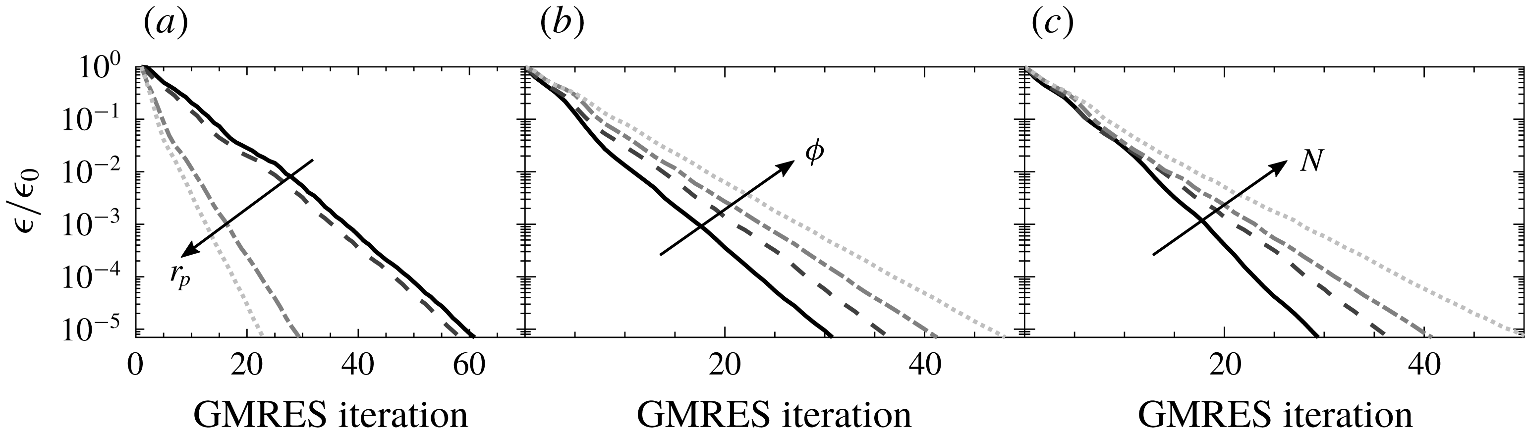
, which originate with the most narrowly separated particles, and that rather small values of
 $r_{p}$
are sufficient to accelerate convergence. The preconditioner is
 $$\begin{eqnarray}{\mathcal{P}}=\left[\begin{array}{@{}cc@{}}\unicode[STIX]{x1D644} & \mathbf{0}\\ {\mathcal{B}}^{\text{T}} & \unicode[STIX]{x1D644}\end{array}\right]\boldsymbol{\cdot }\left[\begin{array}{@{}cc@{}}\unicode[STIX]{x1D701}^{-1}\unicode[STIX]{x1D644} & \mathbf{0}\\ \boldsymbol{ 0} & {\mathcal{L}}\boldsymbol{\cdot }{\mathcal{L}}^{\text{T}}\end{array}\right]\boldsymbol{\cdot }\left[\begin{array}{@{}cc@{}}\unicode[STIX]{x1D644} & {\mathcal{B}}\\ \mathbf{0} & \unicode[STIX]{x1D644}\end{array}\right],\end{eqnarray}$$
and its inverse
 $$\begin{eqnarray}{\mathcal{P}}^{-1}=\left[\begin{array}{@{}cc@{}}\unicode[STIX]{x1D644} & -{\mathcal{B}}\\ \mathbf{0} & \unicode[STIX]{x1D644}\end{array}\right]\boldsymbol{\cdot }\left[\begin{array}{@{}cc@{}}\unicode[STIX]{x1D701}\unicode[STIX]{x1D644} & \mathbf{0}\\ \mathbf{0} & {\mathcal{L}}^{-\text{T}}\boldsymbol{\cdot }{\mathcal{L}}^{-1}\end{array}\right]\boldsymbol{\cdot }\left[\begin{array}{@{}cc@{}}\unicode[STIX]{x1D644} & \mathbf{0}\\ -{\mathcal{B}}^{\text{T}} & \unicode[STIX]{x1D644}\end{array}\right],\end{eqnarray}$$
can be quickly and inexpensively applied to a vector using the triangular solves of
 ${\mathcal{L}}$
and the simple projector
 ${\mathcal{B}}$
.
2.2 Brownian dynamics in the saddle point formulation
In the SD framework, the stochastic force
 $\boldsymbol{F}^{B}$
is also decomposed into near-field and far-field parts (Banchio & Brady Reference Banchio and Brady2003)
 $$\begin{eqnarray}\boldsymbol{F}^{B}=\boldsymbol{F}_{nf}^{B}+\boldsymbol{F}_{ff}^{B},\end{eqnarray}$$
where
 $$\begin{eqnarray}\boldsymbol{F}_{nf}^{B}=\sqrt{\frac{2k_{B}T}{\unicode[STIX]{x0394}t}}(\unicode[STIX]{x1D64D}_{FU}^{nf})^{1/2}\boldsymbol{\cdot }\unicode[STIX]{x1D733}_{nf}\end{eqnarray}$$
and
 $$\begin{eqnarray}\boldsymbol{F}_{ff}^{B}=\sqrt{\frac{2k_{B}T}{\unicode[STIX]{x0394}t}}({\mathcal{B}}^{\text{T}}\boldsymbol{\cdot }{\mathcal{M}}^{-1}\boldsymbol{\cdot }{\mathcal{B}})^{1/2}\boldsymbol{\cdot }\unicode[STIX]{x1D733}_{ff},\end{eqnarray}$$
where
 $\unicode[STIX]{x1D733}_{nf}$
and
 $\unicode[STIX]{x1D733}_{ff}$
are vectors of standard independent Gaussian random variables. The stochastic quantities can also be represented as stochastic variables with zero mean and a covariance set by the fluctuation dissipation theorem, namely
 $$\begin{eqnarray}\displaystyle & \displaystyle \langle \boldsymbol{F}_{nf}^{B}(\text{i}\unicode[STIX]{x0394}t)\boldsymbol{F}_{nf}^{B}(j\unicode[STIX]{x0394}t)\rangle =\frac{2k_{B}T}{\unicode[STIX]{x0394}t}\unicode[STIX]{x1D64D}_{FU}^{nf}\unicode[STIX]{x1D6FF}_{ij}, & \displaystyle\end{eqnarray}$$
 $$\begin{eqnarray}\displaystyle & \displaystyle \langle \boldsymbol{F}_{ff}^{B}(\text{i}\unicode[STIX]{x0394}t)\boldsymbol{F}_{ff}^{B}(j\unicode[STIX]{x0394}t)\rangle =\frac{2k_{B}T}{\unicode[STIX]{x0394}t}{\mathcal{B}}^{\text{T}}\boldsymbol{\cdot }{\mathcal{M}}^{-1}\boldsymbol{\cdot }{\mathcal{B}}\unicode[STIX]{x1D6FF}_{ij}, & \displaystyle\end{eqnarray}$$
where the angle brackets denote an ensemble average over realizations of the stochastic variables and
 $\unicode[STIX]{x1D6FF}_{ij}$
is the Kronecker delta. In this way, computing
 $\boldsymbol{F}_{nf}^{B}$
and
 $\boldsymbol{F}_{ff}^{B}$
can be thought of as generating samples of an instantaneously correlated random vector whose covariance is proportional to a specific matrix. The near-field Brownian forces in (2.15) are reasonably straightforward to compute because the near-field resistance tensor is known and can be directly computed. The far-field Brownian forces, however, are more challenging because the far-field interactions are described in terms of the mobility, whose inverse is therefore required to compute the forces, as shown in (2.16). Banchio & Brady (Reference Banchio and Brady2003) compute these forces directly using the Chebyshev polynomial approximation developed by Fixman (Reference Fixman1986), which is computationally expensive because
 ${\mathcal{M}}$
is ill-conditioned. The saddle point formulation enables a more efficient approach, namely the computation of a far-field slip velocity
 $$\begin{eqnarray}{\mathcal{U}}^{B}=\sqrt{\frac{2k_{B}T}{\unicode[STIX]{x0394}t}}{\mathcal{M}}^{1/2}\boldsymbol{\cdot }\hat{\unicode[STIX]{x1D733}}_{ff},\end{eqnarray}$$
that emerges by rearranging (2.8) to give
 $$\begin{eqnarray}\left[\begin{array}{@{}cc@{}}{\mathcal{M}} & {\mathcal{B}}\\ {\mathcal{B}}^{\text{T}} & -\unicode[STIX]{x1D64D}_{FU}^{nf}\end{array}\right]\boldsymbol{\cdot }\left[\begin{array}{@{}c@{}}\hat{{\mathcal{F}}}\\ \boldsymbol{U}\end{array}\right]=\left[\begin{array}{@{}c@{}}{\mathcal{U}}^{B}\\ -(\boldsymbol{F}^{P}+\boldsymbol{F}_{nf}^{B})\end{array}\right],\end{eqnarray}$$
where
 $\hat{{\mathcal{F}}}={\mathcal{F}}+{\mathcal{M}}^{-1}\boldsymbol{\cdot }{\mathcal{U}}^{B}$
is the set of far-field hydrodynamic forces plus an additional force required to satisfy the no-slip boundary condition on the particle surfaces and
 $\hat{\unicode[STIX]{x1D733}}_{ff}$
is another white noise vector. Introducing
 ${\mathcal{U}}^{B}$
in this way is physically equivalent to imposing a fluctuating stress in the far-field model of the fluid, whose associated particle displacements satisfy the fluctuation–dissipation theorem. For many representations of
 ${\mathcal{M}}$
,
 ${\mathcal{U}}^{B}$
is far easier to compute than
 $\boldsymbol{F}_{ff}^{B}$
, and accelerated techniques with
 $O(N)$
or nearly
 $O(N)$
scaling have been developed for various approximations to
 ${\mathcal{M}}$
. Examples include the fluctuating immersed boundary method published by Delong et al. (Reference Delong, Usabiaga, Delgado-Buscalioni, Griffith and Donev2014), the fluctuating force coupling method of Delmotte & Keaveny (Reference Delmotte and Keaveny2015) and our own positively split Ewald approach (Fiore et al.
Reference Fiore, Usabiaga, Donev and Swan2017; Fiore & Swan Reference Fiore and Swan2018).
Others have also used the concept of a far-field slip velocity to efficiently model the thermal motion of dispersed particles. For example, Delmotte & Keaveny (Reference Delmotte and Keaveny2015) considered spherical particles with force, torques and stresslets, and introduced a slip velocity that included a non-zero rate of strain on each particle. Sprinkle et al. (Reference Sprinkle, Balboa Usabiaga, Patankar and Donev2017) considered rigid multi-blob particles and introduced a fluid slip velocity in an approach that is a special case of the one presented here. In particular, equation (6) in their paper is the special case of (2.20) in which lubrication interactions are neglected and
 ${\mathcal{B}}$
represents their geometric block matrix,
 $-{\mathcal{K}}$
, describing rigid body motions. While the saddle point matrix equation has been previously used by Sprinkle et al. (Reference Sprinkle, Balboa Usabiaga, Patankar and Donev2017) and others in the context of hydrodynamic mobility problems, equation (2.20) is the first time these ideas have been applied to SD or resistance-type problems, in which fluctuating and deterministic near-field forces also need be considered. Equation (2.20) represents a completely general framework for SD simulations of arbitrary particle shapes with relatively few restrictions on the model imposed for near-field HI. No prescription on the particle sizes or shapes has been made, and the method is valid for any symmetric positive semi-definite approximations for
 ${\mathcal{M}}$
and
 $\unicode[STIX]{x1D64D}_{FU}^{nf}$
. In §§ 3 and 4 we discuss techniques specific to spherical particles in periodic geometries, both for computing the deterministic HI and the stochastic forces and slip velocities.
2.3 Stochastic sampling preconditioning
As mentioned in the previous section, accelerated sampling methods for the effective far-field Brownian force can be developed by leveraging the algebraic structure of various approximations for
 ${\mathcal{M}}$
to generate a far-field slip velocity which is then projected onto the set of hydrodynamic constraints. Further discussion of such methods is deferred to § 4. In this section, we describe an efficient and completely general approach to sample the near-field Brownian forces. This approach relies on the iterative Krylov subspace approximations of Chow & Saad (Reference Chow and Saad2014) and leverages the preconditioner that was already developed in § 2.1 for the saddle point problem.
The preconditioning is more simply described using an alternative, but equivalent, notation for the stochastic variables, where an arbitrary random vector
 $\boldsymbol{x}$
drawn from a normal distribution with mean
 $\langle \boldsymbol{x}(\text{i}\unicode[STIX]{x0394}t)\rangle =\unicode[STIX]{x1D741}$
and covariance
 $\langle \boldsymbol{x}(\text{i}\unicode[STIX]{x0394}t)\boldsymbol{x}^{\text{T}}(j\unicode[STIX]{x0394}t)\rangle =\boldsymbol{V}\unicode[STIX]{x1D6FF}_{ij}$
is denoted as
 $$\begin{eqnarray}\boldsymbol{x}\sim {\mathcal{N}}(\unicode[STIX]{x1D741},\boldsymbol{V}).\end{eqnarray}$$
Standard random number generators are only able to draw random samples with a covariance proportional to
 $\unicode[STIX]{x1D644}$
,
 $$\begin{eqnarray}\boldsymbol{n}\sim {\mathcal{N}}(\unicode[STIX]{x1D741},\unicode[STIX]{x1D6FC}\unicode[STIX]{x1D644}),\end{eqnarray}$$
where
 $\unicode[STIX]{x1D6FC}$
is a positive scalar. Sampling a distribution with arbitrary covariance
 $\boldsymbol{V}$
is achieved by computing the product of the square root of the covariance matrix with the independent and identically distributed vector
 $\boldsymbol{n}$
computed the random number generator
 $$\begin{eqnarray}\boldsymbol{x}=\unicode[STIX]{x1D741}+\boldsymbol{V}^{1/2}\boldsymbol{\cdot }\boldsymbol{n}.\end{eqnarray}$$
If
 $\boldsymbol{V}$
is known explicitly, direct calculation of
 $\boldsymbol{V}^{1/2}$
can be evaluated with eigenvalue or singular value decomposition, incurring a computational cost of
 $O(N^{3})$
. Iterative Krylov subspace approximations for
 $\boldsymbol{V}^{1/2}\boldsymbol{\cdot }\boldsymbol{n}$
, such as the commonly used Chebyshev polynomial approach of Fixman (Reference Fixman1986) and the more recently developed Lanczos method of Chow & Saad (Reference Chow and Saad2014), can be applied for an arbitrary
 $\boldsymbol{V}$
. While these iterative schemes may converge even for ill-conditioned matrices, they are especially efficient when
 $\boldsymbol{V}$
is well-conditioned and
 $\boldsymbol{V}\boldsymbol{\cdot }\boldsymbol{x}$
can be rapidly computed. Preconditioning can be used to improve the condition number and accelerate convergence. We will show how this can be achieved to sample
 $\unicode[STIX]{x1D64D}_{FU}^{nf}$
.
Important to any sampling approach is that
 $\unicode[STIX]{x1D64D}_{FU}^{nf}$
is positive semi-definite, which guarantees that the resulting forces are real-valued. Preconditioning is necessary because
 $\unicode[STIX]{x1D64D}_{FU}^{nf}$
is ill-conditioned. The large condition number arises because it has both very large eigenvalues originating in the divergent forces between nearly touching particles and very small eigenvalues for particles with few neighbours whose separations are close to the near-field cutoff radius, and whose entries in the resistance tensor are nearly zero. The large and small eigenvalues are most effectively preconditioned independently.
The preconditioner developed in § 2.1 is primarily designed to condition the large eigenvalues present in
 $\unicode[STIX]{x1D64D}_{FU}^{nf}$
, so it can be recycled here with some careful modifications that ensure the resulting variables have the proper covariance. Here, the relevant piece of the saddle point preconditioner is the incomplete Cholesky factor
 ${\mathcal{L}}$
of the matrix
 $\unicode[STIX]{x1D64B}\boldsymbol{\cdot }(\unicode[STIX]{x1D64D}_{FU}^{nf}+\unicode[STIX]{x1D701}\unicode[STIX]{x1D644})\boldsymbol{\cdot }\unicode[STIX]{x1D64B}^{\text{T}}$
, which is applied to
 $\unicode[STIX]{x1D64D}_{FU}^{nf}$
symmetrically in order to reduce the magnitude of the large eigenvalues,
 $$\begin{eqnarray}{\mathcal{L}}^{-1}\boldsymbol{\cdot }\unicode[STIX]{x1D64B}\boldsymbol{\cdot }\unicode[STIX]{x1D64D}_{FU}^{nf}\boldsymbol{\cdot }\unicode[STIX]{x1D64B}^{\text{T}}\boldsymbol{\cdot }{\mathcal{L}}^{-\text{T}}.\end{eqnarray}$$
To precondition the small eigenvalues, we use a diagonal matrix that is designed to scale each row and column of
 $\unicode[STIX]{x1D64D}_{FU}^{nf}$
with suitably small non-zero diagonals,
 $0<(\unicode[STIX]{x1D64D}_{FU}^{nf})_{ii}<\unicode[STIX]{x1D701}$
, by the diagonal element, so that the relative magnitude of the entries within each row and column is preserved but the absolute magnitudes cluster around
 $\unicode[STIX]{x1D701}$
. This preconditioner does not alter the rows and columns of
 $\unicode[STIX]{x1D64D}_{FU}^{nf}$
with diagonals that are either zero or greater than or equal to a nominal drag coefficient, say
 $\unicode[STIX]{x1D701}=6\unicode[STIX]{x03C0}\unicode[STIX]{x1D702}a$
for mono-disperse spherical particles, i.e.
 $$\begin{eqnarray}\unicode[STIX]{x1D60B}_{ii}=\left\{\begin{array}{@{}ll@{}}(\unicode[STIX]{x1D64D}_{FU}^{nf})_{ii}^{1/2}, & 0<(\unicode[STIX]{x1D64D}_{FU}^{nf})_{ii}<6\unicode[STIX]{x03C0}\unicode[STIX]{x1D702}a,\\ 1, & (\unicode[STIX]{x1D64D}_{FU}^{nf})_{ii}=0,\\ 1, & (\unicode[STIX]{x1D64D}_{FU}^{nf})_{ii}\geqslant 6\unicode[STIX]{x03C0}\unicode[STIX]{x1D702}a.\end{array}\right.\end{eqnarray}$$
Here,
 $\unicode[STIX]{x1D63F}$
is primarily expected to be important at low particle volume fractions, for which particles are more likely to be well separated and have only a few neighbours within the near-field cutoff radius. Combining this preconditioner with the incomplete Cholesky preconditioner for large eigenvalues yields the preconditioned matrix
 $$\begin{eqnarray}{\mathcal{L}}^{-1}\boldsymbol{\cdot }\unicode[STIX]{x1D64B}\boldsymbol{\cdot }\unicode[STIX]{x1D63F}^{-1}\boldsymbol{\cdot }\unicode[STIX]{x1D64D}_{FU}^{nf}\boldsymbol{\cdot }\unicode[STIX]{x1D63F}^{-\text{T}}\boldsymbol{\cdot }\unicode[STIX]{x1D64B}^{\text{T}}\boldsymbol{\cdot }{\mathcal{L}}^{-\text{T}}.\end{eqnarray}$$
Unfortunately, this preconditioner is not a great approximation for
 $\unicode[STIX]{x1D64D}_{FU}^{nf}$
because
 $\unicode[STIX]{x1D64D}_{FU}^{nf}$
only has non-zero rows for particles that are closely separated, whereas the addition of
 $\unicode[STIX]{x1D701}\boldsymbol{I}$
in the computation of
 ${\mathcal{L}}$
guarantees that
 ${\mathcal{L}}$
has no rows or columns that are purely zero. The effect of the preconditioner can be improved by instead sampling forces from the distribution
 $$\begin{eqnarray}\hat{\boldsymbol{F}}_{nf}^{B}\sim {\mathcal{N}}\left(\mathbf{0},\frac{2k_{B}T}{\unicode[STIX]{x0394}t}(\unicode[STIX]{x1D64D}_{FU}^{nf}+\unicode[STIX]{x1D701}\unicode[STIX]{x1D644}_{nn})\right),\end{eqnarray}$$
where
 $\unicode[STIX]{x1D644}_{nn}$
is a modified identity tensor with ones where the diagonal elements of
 $\unicode[STIX]{x1D64D}_{FU}^{nf}$
are zero, i.e. for the rows/columns associated with neighbourless particles, and zero otherwise, i.e.
 $$\begin{eqnarray}(\unicode[STIX]{x1D644}_{nn})_{ii}=\left\{\begin{array}{@{}ll@{}}1, & (\unicode[STIX]{x1D64D}_{FU}^{nf})_{ii}=0,\\ 0, & (\unicode[STIX]{x1D64D}_{FU}^{nf})_{ii}\neq 0.\end{array}\right.\end{eqnarray}$$
Neighbourless particles experience no near-field Brownian force, so the proper force distribution can be obtained by projecting the corresponding elements of
 $\boldsymbol{F}_{nf}^{B}$
to zero
 $$\begin{eqnarray}\boldsymbol{F}_{nf}^{B}=(\unicode[STIX]{x1D644}-\unicode[STIX]{x1D644}_{nn})\boldsymbol{\cdot }\hat{\boldsymbol{F}}_{nf}^{B}\sim {\mathcal{N}}\left(\mathbf{0},\frac{2k_{B}T}{\unicode[STIX]{x0394}t}\unicode[STIX]{x1D64D}_{FU}^{nf}\right).\end{eqnarray}$$
The operator
 $(\unicode[STIX]{x1D644}-\unicode[STIX]{x1D644}_{nn})$
is a projector that removes the additional noise introduced by adding
 $\unicode[STIX]{x1D701}\unicode[STIX]{x1D644}_{nn}$
to
 $\unicode[STIX]{x1D64D}_{FU}^{nf}$
. This operation works because we project out a subset of the Brownian forces. The preconditioned sampling produces random vectors
 $$\begin{eqnarray}\boldsymbol{z}\sim {\mathcal{N}}\left(\mathbf{0},\frac{2k_{B}T}{\unicode[STIX]{x0394}t}{\mathcal{L}}^{-1}\boldsymbol{\cdot }\unicode[STIX]{x1D64B}\boldsymbol{\cdot }\unicode[STIX]{x1D63F}^{-1}\boldsymbol{\cdot }(\unicode[STIX]{x1D64D}_{FU}^{nf}+\unicode[STIX]{x1D701}\unicode[STIX]{x1D644}_{nn})\boldsymbol{\cdot }\unicode[STIX]{x1D63F}^{-\text{T}}\boldsymbol{\cdot }\unicode[STIX]{x1D64B}^{\text{T}}\boldsymbol{\cdot }{\mathcal{L}}^{-\text{T}}\right),\end{eqnarray}$$
where
 $$\begin{eqnarray}\boldsymbol{F}_{nf}^{B}=(\unicode[STIX]{x1D644}-\unicode[STIX]{x1D644}_{nn})\boldsymbol{\cdot }\unicode[STIX]{x1D63F}\boldsymbol{\cdot }\unicode[STIX]{x1D64B}^{\text{T}}\boldsymbol{\cdot }{\mathcal{L}}\boldsymbol{\cdot }\boldsymbol{z}\sim {\mathcal{N}}\left(\mathbf{0},\frac{2k_{B}T}{\unicode[STIX]{x0394}t}\unicode[STIX]{x1D64D}_{FU}^{nf}\right).\end{eqnarray}$$
The use of
 $\unicode[STIX]{x1D644}_{nn}$
and
 $\unicode[STIX]{x1D644}-\unicode[STIX]{x1D644}_{nn}$
bears some additional discussion. As mentioned, adding
 $\unicode[STIX]{x1D644}_{nn}$
to
 $\unicode[STIX]{x1D64D}_{FU}^{nf}$
improves the efficacy of the incomplete Cholesky preconditioner but increases the variance of the stochastic forces. Fortunately, particles that have no neighbours in the near field cannot experience a near-field Brownian force; the operator
 $\unicode[STIX]{x1D644}-\unicode[STIX]{x1D644}_{nn}$
projects these forces out of
 $\boldsymbol{F}_{nf}^{B}$
and restores the expected covariance. This approach only works because those forces should be exactly zero. Additional preconditioning may be possible for specific forms of
 $\unicode[STIX]{x1D64D}_{FU}^{nf}$
, where knowledge of the specific interactions can be used to further compress the eigenspectrum and improve convergence. The efficacy of the preconditioner presented in this section is demonstrated in § 4 for the Stokesian dynamics lubrication approximation for the near-field resistance.
It is important to note that the approach advocated in this section is not the same as simply omitting the particles that have no neighbours. Rather, Brownian forces are computed for all particles then projected onto the set of particles with neighbours. The motivation behind this approach is to leverage the preconditioner already developed for the saddle point problem in § 2.1, which effectively preconditions many of the features that contribute to large and small eigenvalues in the covariance matrix of the stochastic sampling problem, so as to avoid repeating those calculations. In order to use the saddle point preconditioner, which considers all particles and not solely the ones with neighbours, the Brownian sampling method must at some stage generate noise for these particles without neighbours.
3 Hydrodynamic models
3.1 Far-field hydrodynamics for monodisperse spheres
The far-field mobility tensor
 ${\mathcal{M}}$
is constructed by multipole expansion. We have previously developed a compact representation of
 ${\mathcal{M}}$
(Fiore et al.
Reference Fiore, Usabiaga, Donev and Swan2017; Fiore & Swan Reference Fiore and Swan2018), which will be summarized here for completeness. Equivalent representations have also been developed by Ladd (Reference Ladd1990) and Mizerski et al. (Reference Mizerski, Wajnryb, Zuk and Szymczak2014). This representation is derived from the integral formulation of the Stokes equations for rigid suspended bodies (Ladyzhenskaya & Silverman Reference Ladyzhenskaya and Silverman1969)
 $$\begin{eqnarray}u_{i}(\boldsymbol{x})=\int _{S_{\unicode[STIX]{x1D6FD}}}\text{d}S_{\unicode[STIX]{x1D6FD}}(\,\boldsymbol{y})\unicode[STIX]{x1D611}_{im}(\boldsymbol{x},\boldsymbol{y})f_{m}(\,\boldsymbol{y}),\end{eqnarray}$$
where
 $u_{i}(\boldsymbol{x})$
is the
 $i$
th component of the fluid velocity at a point
 $\boldsymbol{x}$
in the fluid propagated by the force density
 $\boldsymbol{f}(\,\boldsymbol{y})$
at point
 $\boldsymbol{y}$
on the particle surface
 $S_{\unicode[STIX]{x1D6FD}}$
through the Green’s function
 $\unicode[STIX]{x1D645}$
. In this and following equations, Einstein summation notation is assumed for repeated indices. All particles are assumed to be spherical and the first few multipole moments are used to approximate the force density on the surface of each particle
 $$\begin{eqnarray}f_{j}=\frac{1}{4\unicode[STIX]{x03C0}a^{2}}F_{j}+\frac{3}{4\unicode[STIX]{x03C0}a^{3}}\hat{n}_{n}C_{nj}+\cdots ,\end{eqnarray}$$
where
 $\hat{\boldsymbol{n}}$
is the normal to the particle surface,
 $a$
is the particle radius,
 $\boldsymbol{F}$
is the total force on the particle and
 $\boldsymbol{C}$
is the traceless couplet, whose symmetric and antisymmetric components are the stresslet and torque, respectively. The multipole expansion is truncated after the couplet for computational efficiency, but can in principle be extended to arbitrary order. The force and couplet are defined by
 $$\begin{eqnarray}\displaystyle & \displaystyle F_{m}=\int _{S_{\unicode[STIX]{x1D6FD}}}\,\text{d}S_{\unicode[STIX]{x1D6FD}}\,f_{m}, & \displaystyle\end{eqnarray}$$
 $$\begin{eqnarray}\displaystyle & \displaystyle C_{mn}=\int _{S_{\unicode[STIX]{x1D6FD}}}\,\text{d}S_{\unicode[STIX]{x1D6FD}}\left[(y_{m}-x_{\unicode[STIX]{x1D6FD},m})f_{n}-{\textstyle \frac{1}{3}}\unicode[STIX]{x1D6FF}_{mn}(y_{p}-x_{\unicode[STIX]{x1D6FD},p})f_{p}\right], & \displaystyle\end{eqnarray}$$
where
 $\boldsymbol{x}_{\unicode[STIX]{x1D6FD}}$
is the location of the centre of particle
 $\unicode[STIX]{x1D6FD}$
, and higher-order moments are defined by higher-order outer products of the distance vector
 $(\,\boldsymbol{y}-\boldsymbol{x})$
with
 $\boldsymbol{f}$
. Faxeń laws infer particle motion in response to the stresses exerted on its surface by a flow field, and are effectively integral statements of the no-slip boundary condition,
 $$\begin{eqnarray}\displaystyle & \displaystyle U_{i}=\frac{1}{4\unicode[STIX]{x03C0}a^{2}}\int _{S_{\unicode[STIX]{x1D6FC}}}\,\text{d}S_{\unicode[STIX]{x1D6FC}}(\boldsymbol{x})u_{i}(\boldsymbol{x}), & \displaystyle\end{eqnarray}$$
 $$\begin{eqnarray}\displaystyle & \displaystyle \unicode[STIX]{x1D60B}_{ij}=\frac{3}{4\unicode[STIX]{x03C0}a^{3}}\int _{S_{\unicode[STIX]{x1D6FC}}}\,\text{d}S_{\unicode[STIX]{x1D6FC}}(\boldsymbol{x})u_{i}\hat{n}_{j}, & \displaystyle\end{eqnarray}$$
where
 $S_{\unicode[STIX]{x1D6FC}}$
is the surface of particle
 $\unicode[STIX]{x1D6FC}$
, and
 $V_{\unicode[STIX]{x1D6FC}}$
is its volume. The particle velocity gradient,
 $\unicode[STIX]{x1D63F}$
, is composed of a symmetric part, the rate of strain
 $\boldsymbol{E}$
, and an anti-symmetric part, the angular velocity
 $\unicode[STIX]{x1D734}$
.
The linearity of the Stokes equations allows independent coupling and superposition of the total force or couplet to the velocity or velocity gradient. Substituting the fluid velocity (3.1) and the multipole expansion (3.2) into the Faxén laws (3.5), (3.6) gives the following relations between the force moments on particle
 $\unicode[STIX]{x1D6FD}$
and the velocity moments induced on particle
 $\unicode[STIX]{x1D6FC}$
 $$\begin{eqnarray}\left[\begin{array}{@{}c@{}}U_{i}^{\unicode[STIX]{x1D6FC}}\\ \unicode[STIX]{x1D60B}_{ij}^{\unicode[STIX]{x1D6FC}}\end{array}\right]=\left[\begin{array}{@{}cc@{}}\unicode[STIX]{x1D614}_{UF,im}^{\unicode[STIX]{x1D6FC}\unicode[STIX]{x1D6FD}} & \unicode[STIX]{x1D614}_{UC,imn}^{\unicode[STIX]{x1D6FC}\unicode[STIX]{x1D6FD}}\\ \unicode[STIX]{x1D614}_{DF,ijm}^{\unicode[STIX]{x1D6FC}\unicode[STIX]{x1D6FD}} & \unicode[STIX]{x1D614}_{DC,ijmn}^{\unicode[STIX]{x1D6FC}\unicode[STIX]{x1D6FD}}\end{array}\right]\boldsymbol{\cdot }\left[\begin{array}{@{}c@{}}F_{m}^{\unicode[STIX]{x1D6FD}}\\ C_{mn}^{\unicode[STIX]{x1D6FD}}\end{array}\right],\end{eqnarray}$$
where the elements of the pair mobility tensors are given in terms of integrals of the Green’s function over the particle surfaces
 $$\begin{eqnarray}\displaystyle & \displaystyle \unicode[STIX]{x1D614}_{UF,im}^{\unicode[STIX]{x1D6FC}\unicode[STIX]{x1D6FD}}=\frac{1}{4\unicode[STIX]{x03C0}a^{2}}\int _{S_{\unicode[STIX]{x1D6FC}}}\,\text{d}S_{\unicode[STIX]{x1D6FC}}(\boldsymbol{x})\frac{1}{4\unicode[STIX]{x03C0}a^{2}}\int _{S_{\unicode[STIX]{x1D6FD}}}\,\text{d}S_{\unicode[STIX]{x1D6FD}}(\,\boldsymbol{y})\unicode[STIX]{x1D611}_{im}(\boldsymbol{x},\boldsymbol{y}), & \displaystyle\end{eqnarray}$$
 $$\begin{eqnarray}\displaystyle & \displaystyle \unicode[STIX]{x1D614}_{UC,imn}^{\unicode[STIX]{x1D6FC}\unicode[STIX]{x1D6FD}}=\frac{1}{4\unicode[STIX]{x03C0}a^{2}}\int _{S_{\unicode[STIX]{x1D6FC}}}\,\text{d}S_{\unicode[STIX]{x1D6FC}}(\boldsymbol{x})\frac{3}{4\unicode[STIX]{x03C0}a^{3}}\int _{S_{\unicode[STIX]{x1D6FD}}}\,\text{d}S_{\unicode[STIX]{x1D6FD}}(\,\boldsymbol{y})\unicode[STIX]{x1D611}_{im}(\boldsymbol{x},\boldsymbol{y})\hat{n}_{n}^{\unicode[STIX]{x1D6FD}}, & \displaystyle\end{eqnarray}$$
 $$\begin{eqnarray}\displaystyle & \displaystyle \unicode[STIX]{x1D614}_{DF,ijm}^{\unicode[STIX]{x1D6FC}\unicode[STIX]{x1D6FD}}=\frac{3}{4\unicode[STIX]{x03C0}a^{3}}\int _{S_{\unicode[STIX]{x1D6FC}}}\,\text{d}S_{\unicode[STIX]{x1D6FC}}(\boldsymbol{x})\hat{n}_{j}^{\unicode[STIX]{x1D6FC}}\frac{1}{4\unicode[STIX]{x03C0}a^{2}}\int _{S_{\unicode[STIX]{x1D6FD}}}\,\text{d}S_{\unicode[STIX]{x1D6FD}}(\,\boldsymbol{y})\unicode[STIX]{x1D611}_{im}(\boldsymbol{x},\boldsymbol{y}), & \displaystyle\end{eqnarray}$$
 $$\begin{eqnarray}\displaystyle & \displaystyle \unicode[STIX]{x1D614}_{DC,ijmn}^{\unicode[STIX]{x1D6FC}\unicode[STIX]{x1D6FD}}=\frac{3}{4\unicode[STIX]{x03C0}a^{3}}\int _{S_{\unicode[STIX]{x1D6FC}}}\,\text{d}S_{\unicode[STIX]{x1D6FC}}(\boldsymbol{x})\hat{n}_{j}^{\unicode[STIX]{x1D6FC}}\frac{3}{4\unicode[STIX]{x03C0}a^{3}}\int _{S_{\unicode[STIX]{x1D6FD}}}\,\text{d}S_{\unicode[STIX]{x1D6FD}}(\,\boldsymbol{y})\unicode[STIX]{x1D611}_{im}(\boldsymbol{x},\boldsymbol{y})\hat{n}_{n}^{\unicode[STIX]{x1D6FD}}. & \displaystyle\end{eqnarray}$$
For periodic systems, which are commonly used in simulation, the appropriate Green’s function is given by Hasimoto (Reference Hasimoto1959),
 $$\begin{eqnarray}\unicode[STIX]{x1D645}(\boldsymbol{x},\boldsymbol{y})=\frac{1}{\unicode[STIX]{x1D702}V}\mathop{\sum }_{\boldsymbol{k}\neq \mathbf{0}}\text{e}^{\text{i}\boldsymbol{k}\boldsymbol{\cdot }(\boldsymbol{x}-\boldsymbol{y})}\frac{1}{k^{2}}(\unicode[STIX]{x1D644}-\hat{\boldsymbol{k}}\hat{\boldsymbol{k}}),\end{eqnarray}$$
where
 $\unicode[STIX]{x1D645}(\boldsymbol{x},\boldsymbol{y})\boldsymbol{\cdot }\boldsymbol{F}$
is the fluid velocity at point
 $\boldsymbol{x}$
propagated by a force
 $\boldsymbol{F}$
located at point
 $\boldsymbol{y}$
and its periodic images on a lattice,
 $\unicode[STIX]{x1D644}$
is the identity tensor,
 $\boldsymbol{k}$
are drawn from the set of reciprocal (Fourier) space lattice vectors excluding the zero vector,
 $\unicode[STIX]{x1D702}$
is fluid viscosity and
 $V$
is the periodic cell volume. With Hasimoto’s solution, the integrals in (3.8)–(3.11) can be evaluated in principle. The integrals do not necessarily have analytically tractable solutions for arbitrary particle shapes, but are straightforward to evaluate for spherical particles, which are the focus of this work. Substituting (3.12) into (3.8)–(3.11) and evaluating the surface integrals in Fourier space gives algebraic expressions for the pair mobilities of spherical particles with equal, finite size
 $$\begin{eqnarray}\unicode[STIX]{x1D648}_{pq}^{\unicode[STIX]{x1D6FC}\unicode[STIX]{x1D6FD}}=\frac{1}{\unicode[STIX]{x1D702}V}\mathop{\sum }_{\boldsymbol{k}\neq \mathbf{0}}\text{e}^{\text{i}\boldsymbol{k}\boldsymbol{\cdot }(\boldsymbol{x}_{\unicode[STIX]{x1D6FC}}-\boldsymbol{x}_{\unicode[STIX]{x1D6FD}})}\frac{1}{k^{2}}\boldsymbol{s}^{p}(ka)(\unicode[STIX]{x1D644}-\hat{\boldsymbol{k}}\hat{\boldsymbol{k}})\boldsymbol{s}^{q}(ka).\end{eqnarray}$$
The shape factors are proportional to spherical Bessel functions of the first kind, and can be related to the order of the moment in the multipole expansion
 $p$
as,
 $$\begin{eqnarray}\boldsymbol{s}^{p}(ka)=(-1)^{p/2}(2p+1)!!\text{j}_{p}(ka)\,\hat{\boldsymbol{k}}^{p},\end{eqnarray}$$
where
 $\hat{\boldsymbol{k}}^{p}$
is an irreducible tensor of rank
 $p$
(Ladd Reference Ladd1990) and
 $\text{j}_{m}(x)$
is the spherical Bessel function of the first kind of order
 $m$
(Abramowitz & Stegun Reference Abramowitz and Stegun1965). The shape factors for the force and linear velocity (
 $p=0$
) are
 $\boldsymbol{s}^{0}(ka)=\text{j}_{0}(ka)$
and the shape factors for the couplet and velocity gradient (
 $p=1$
) are
 $\boldsymbol{s}^{1}(ka)=3\sqrt{-1}\boldsymbol{k}\text{j}_{1}(ka)$
.
The sum in (3.13) is slowly converging, but the convergence can be accelerated using the Ewald sum splitting (Ewald Reference Ewald1921), which filters the slowly decaying, large wavenumber terms out of the sum and explicitly reconstructs them in real space, where they converge quickly because they are associated with high-frequency (short wavelength) motions. Mathematically, the mobility sum
 $\unicode[STIX]{x1D648}_{pq}^{\unicode[STIX]{x1D6FC}\unicode[STIX]{x1D6FD}}=\sum _{\boldsymbol{k}\neq \mathbf{0}}\unicode[STIX]{x1D648}_{k}$
is written in two parts
 $\unicode[STIX]{x1D648}_{pq}^{\unicode[STIX]{x1D6FC}\unicode[STIX]{x1D6FD}}=\sum _{\boldsymbol{k}\neq \mathbf{0}}(1-H(k,\unicode[STIX]{x1D709}))\unicode[STIX]{x1D648}_{k}+\sum _{\boldsymbol{k}\neq \mathbf{0}}H(k,\unicode[STIX]{x1D709})\unicode[STIX]{x1D648}_{k}$
, where the first term is analytically reconstructed in real space by applying the inverse Fourier transform and the second sum is left in wave space. Hasimoto (Reference Hasimoto1959) derived the Ewald sum for periodic Stokes flow using the filter
 $$\begin{eqnarray}H(k,\unicode[STIX]{x1D709})=(1+k^{2}/4\unicode[STIX]{x1D709}^{2})\text{e}^{-k^{2}/4\unicode[STIX]{x1D709}^{2}},\end{eqnarray}$$
and showed that the terms in the resulting real-space sum are exponentially decaying functions of distance, while the terms in the wave-space sum are exponentially decaying functions of wavenumber. The variable
 $\unicode[STIX]{x1D709}$
is an arbitrary parameter that controls how many terms are filtered out of the wave-space sum; in the limit that
 $\unicode[STIX]{x1D709}\rightarrow 0$
, the entire sum is evaluated in real space. Using this filter, the real-space and wave-space contributions to the pair mobility tensor,
 $\unicode[STIX]{x1D648}_{pq}^{\unicode[STIX]{x1D6FC}\unicode[STIX]{x1D6FD}}=(\unicode[STIX]{x1D648}_{pq}^{\unicode[STIX]{x1D6FC}\unicode[STIX]{x1D6FD}})_{r}+(\unicode[STIX]{x1D648}_{pq}^{\unicode[STIX]{x1D6FC}\unicode[STIX]{x1D6FD}})_{w}$
, are respectively
 $$\begin{eqnarray}\displaystyle & \displaystyle (\unicode[STIX]{x1D648}_{pq}^{\unicode[STIX]{x1D6FC}\unicode[STIX]{x1D6FD}})_{r}=\frac{1}{\unicode[STIX]{x1D702}V}\mathop{\sum }_{\boldsymbol{k}\neq \mathbf{0}}\text{e}^{\text{i}\boldsymbol{k}\boldsymbol{\cdot }(\boldsymbol{x}_{\unicode[STIX]{x1D6FC}}-\boldsymbol{x}_{\unicode[STIX]{x1D6FD}})}\frac{1}{k^{2}}(1-H(k,\unicode[STIX]{x1D709}))\boldsymbol{s}^{p}(ka)(\unicode[STIX]{x1D644}-\hat{\boldsymbol{k}}\hat{\boldsymbol{k}})\boldsymbol{s}^{q}(ka), & \displaystyle\end{eqnarray}$$
 $$\begin{eqnarray}\displaystyle & \displaystyle (\unicode[STIX]{x1D648}_{pq}^{\unicode[STIX]{x1D6FC}\unicode[STIX]{x1D6FD}})_{w}=\frac{1}{\unicode[STIX]{x1D702}V}\mathop{\sum }_{\boldsymbol{k}\neq \mathbf{0}}\text{e}^{\text{i}\boldsymbol{k}\boldsymbol{\cdot }(\boldsymbol{x}_{\unicode[STIX]{x1D6FC}}-\boldsymbol{x}_{\unicode[STIX]{x1D6FD}})}\frac{1}{k^{2}}H(k,\unicode[STIX]{x1D709})\boldsymbol{s}^{p}(ka)(\unicode[STIX]{x1D644}-\hat{\boldsymbol{k}}\hat{\boldsymbol{k}})\boldsymbol{s}^{q}(ka). & \displaystyle\end{eqnarray}$$
The real-space representation of the pair mobility tensors are computed by taking the inverse Fourier transform of (3.16) for each set of shape factors. The compact representations of these tensors are
 $$\begin{eqnarray}\displaystyle & \displaystyle (\unicode[STIX]{x1D614}_{UF,im}^{\unicode[STIX]{x1D6FC}\unicode[STIX]{x1D6FD}})_{r}=c_{UF}^{(1)}(r)(\unicode[STIX]{x1D6FF}_{im}-\hat{r}_{i}\hat{r}_{m})+c_{UF}^{(2)}(r)\hat{r}_{i}\hat{r}_{m}, & \displaystyle\end{eqnarray}$$
 $$\begin{eqnarray}\displaystyle & \displaystyle (\unicode[STIX]{x1D614}_{UC,imn}^{\unicode[STIX]{x1D6FC}\unicode[STIX]{x1D6FD}})_{r}=c_{UC}^{(1)}(r)(\unicode[STIX]{x1D6FF}_{im}\hat{r}_{n}-\hat{r}_{i}\hat{r}_{m}\hat{r}_{m})+c_{UC}^{(2)}(r)(\unicode[STIX]{x1D6FF}_{in}\hat{r}_{m}+\unicode[STIX]{x1D6FF}_{mn}\hat{r}_{i}-4\hat{r}_{i}\hat{r}_{m}\hat{r}_{n}), & \displaystyle\end{eqnarray}$$
 $$\begin{eqnarray}\displaystyle (\unicode[STIX]{x1D614}_{DC,ijmn}^{\unicode[STIX]{x1D6FC}\unicode[STIX]{x1D6FD}})_{r} & = & \displaystyle c_{DC}^{(1)}(r)(\unicode[STIX]{x1D6FF}_{ij}\unicode[STIX]{x1D6FF}_{mn}+\unicode[STIX]{x1D6FF}_{im}\unicode[STIX]{x1D6FF}_{jn}-4\unicode[STIX]{x1D6FF}_{in}\unicode[STIX]{x1D6FF}_{jm})+c_{DC}^{(2)}(r)(\unicode[STIX]{x1D6FF}_{jm}\hat{r}_{i}\hat{r}_{n}-\hat{r}_{i}\hat{r}_{j}\hat{r}_{m}\hat{r}_{n})\nonumber\\ \displaystyle & & \displaystyle +\,c_{DC}^{(3)}(r)(\unicode[STIX]{x1D6FF}_{ij}\hat{r}_{m}\hat{r}_{n}+\unicode[STIX]{x1D6FF}_{im}\hat{r}_{j}\hat{r}_{n}+\unicode[STIX]{x1D6FF}_{jn}\hat{r}_{i}\hat{r}_{m}+\unicode[STIX]{x1D6FF}_{mn}\hat{r}_{i}\hat{r}_{j}+\unicode[STIX]{x1D6FF}_{in}\hat{r}_{j}\hat{r}_{m}-6\hat{r}_{i}\hat{r}_{j}\hat{r}_{m}\hat{r}_{n}-\unicode[STIX]{x1D6FF}_{in}\unicode[STIX]{x1D6FF}_{jm}),\nonumber\\ \displaystyle & & \displaystyle\end{eqnarray}$$
where
 $\hat{\boldsymbol{r}}$
is the unit distance vector between the particle centres,
 $r$
is its magnitude,
 $\unicode[STIX]{x1D6FF}_{ij}$
is the Kronecker delta function and the scalar coefficients
 $c_{UF}^{(1)}$
,
 $c_{UF}^{(2)}$
,
 $c_{UC}^{(1)}$
,
 $c_{UC}^{(2)}$
,
 $c_{DC}^{(1)}$
,
 $c_{DC}^{(2)}$
,
 $c_{DC}^{(3)}$
are exponentially decaying functions of the interparticle distance derived by analytically evaluating the inverse Fourier transform and projecting onto a minimal tensor basis. These functions are detailed in our previous work (Fiore & Swan Reference Fiore and Swan2018). It is important to note that the pair mobility tensor presented here, combined with the Hasimoto filter for the Ewald sum applied in Fourier space produces what we term a positive splitting, i.e. a splitting for which the real-space and wave-space contributions to the operator are independently positive semi-definite, as discussed previously (Fiore et al.
Reference Fiore, Usabiaga, Donev and Swan2017; Fiore & Swan Reference Fiore and Swan2018).
The far-field grand mobility tensor, which describes the set of interactions between all particle pairs
 $$\begin{eqnarray}{\mathcal{M}}=\left[\begin{array}{@{}cc@{}}{\mathcal{M}}_{UF} & {\mathcal{M}}_{UC}\\ {\mathcal{M}}_{DF} & {\mathcal{M}}_{DC}\end{array}\right],\end{eqnarray}$$
whose sub-blocks are built from the pair mobility tensors, e.g.
 $$\begin{eqnarray}{\mathcal{M}}_{UF}=\left[\begin{array}{@{}cccc@{}}\unicode[STIX]{x1D648}_{UF}^{11} & \unicode[STIX]{x1D648}_{UF}^{12} & \cdots \, & \unicode[STIX]{x1D648}_{UF}^{1N}\\ \unicode[STIX]{x1D648}_{UF}^{21} & \unicode[STIX]{x1D648}_{UF}^{22} & & \unicode[STIX]{x1D648}_{UF}^{2N}\\ \vdots & & \ddots & \vdots \\ \unicode[STIX]{x1D648}_{UF}^{N1} & \unicode[STIX]{x1D648}_{UF}^{N2} & \cdots \, & \unicode[STIX]{x1D648}_{UF}^{NN}\end{array}\right],\end{eqnarray}$$
is also positive semi-definite for all particle configurations and its Ewald sum
 $$\begin{eqnarray}{\mathcal{M}}={\mathcal{M}}_{r}+{\mathcal{M}}_{w},\end{eqnarray}$$
also represents a positive splitting. This is an important feature and is crucial for fast sampling of the far-field Brownian noise, as discussed in § 4.1.
The wave-space component of the mobility can be written compactly using linear operators
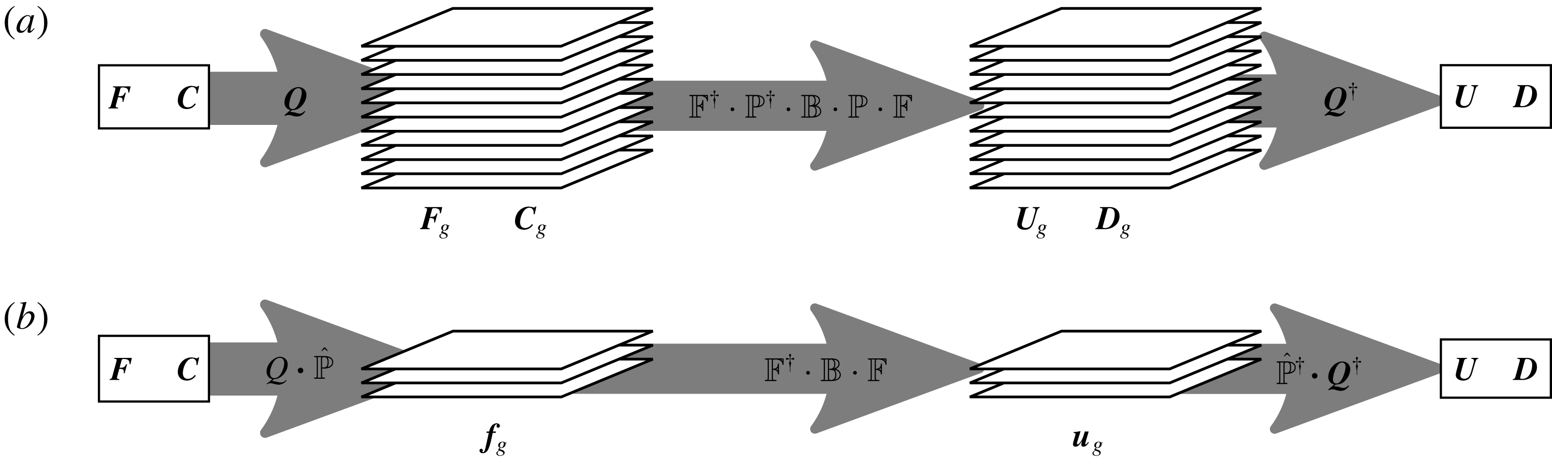
 $$\begin{eqnarray}{\mathcal{M}}_{w}=\mathbb{D}^{\dagger }\boldsymbol{\cdot }\mathbb{P}^{\dagger }\boldsymbol{\cdot }\mathbb{B}\boldsymbol{\cdot }\mathbb{P}\boldsymbol{\cdot }\mathbb{D},\end{eqnarray}$$
where
 $\mathbb{D}$
is the unitary non-uniform discrete Fourier transform (NUDFT) operator, and
 $\mathbb{D}^{\dagger }$
is its adjoint/inverse.
 $\mathbb{D}$
transforms the force moments applied on particles from real space to Fourier space.
 $\mathbb{B}$
is a symmetric block diagonal matrix whose
 $i$
th diagonal block is
 $$\begin{eqnarray}\mathbb{B}_{i}=\frac{H(k_{i},\unicode[STIX]{x1D709})}{\unicode[STIX]{x1D702}Vk_{i}^{2}}(\unicode[STIX]{x1D644}-\hat{\boldsymbol{k}}_{i}\hat{\boldsymbol{k}}_{i}),\end{eqnarray}$$
where
 $\hat{\boldsymbol{k}}_{i}$
is
 $i$
th wavevector;
 $\mathbb{B}$
multiplies the Fourier components of the force by the Green’s function
 $1/\unicode[STIX]{x1D702}Vk_{i}^{2}$
and Hasimoto
 $H(k_{i},\unicode[STIX]{x1D709})$
scaling factors and projects them onto the space of divergence-free velocity fields via the orthogonal projector
 $(\unicode[STIX]{x1D644}-\hat{\boldsymbol{k}}\hat{\boldsymbol{k}})$
. The projector
 $\mathbb{P}$
contains the non-negative shape factors that map the Fourier-space force moments onto the force density, and its adjoint
 $\mathbb{P}^{\dagger }$
maps the Fourier-space velocity field onto the Fourier-space velocity moments;
 $\mathbb{P}$
is a rectangular matrix whose only non-zero entries are rectangular blocks along the main diagonal,
 $$\begin{eqnarray}\mathbb{P}_{i}=\left[\begin{array}{@{}cc@{}}\,\text{j}_{0}(k_{i}a)\unicode[STIX]{x1D644} & 3\sqrt{-1}\text{j}_{1}(k_{i}a)\boldsymbol{k}_{i}\end{array}\right].\end{eqnarray}$$
The matrix
 $\mathbb{P}_{i}^{\dagger }\boldsymbol{\cdot }\mathbb{B}_{i}\boldsymbol{\cdot }\mathbb{P}_{i}$
is the wave-space representation of the mobility tensor at the
 $i$
th wave vector, i.e. the summand in (3.17) except for the exponential factor, where the exponential factors and the sum over
 $\boldsymbol{k}\neq \mathbf{0}$
come from the application of the NUDFT and it inverse,
 $\mathbb{D}$
and
 $\mathbb{D}^{\dagger }$
.
The results presented in this section hold for monodisperse suspensions of spherical particles. Polydispersity can be incorporated in the expressions presented in this section through subtle modifications to the shape factors and scalar functions. This application is discussed in appendix A. Non-spherical particles can be built from rigid assemblies of spherical beads represented using the shape factors presented here. A detailed discussion of this method is deferred to § 6.
3.2 Near-field hydrodynamics
We construct the near-field lubrication tensor
 $\unicode[STIX]{x1D64D}_{\unicode[STIX]{x1D6FC}\unicode[STIX]{x1D6FD}}^{nf}$
separately for each pair of particles
 $\unicode[STIX]{x1D6FC}$
and
 $\unicode[STIX]{x1D6FD}$
whose distance is shorter than a cutoff radius of
 $r_{lub}$
. The exact series expansion for the hydrodynamic resistance between two spheres (Jeffrey & Onishi Reference Jeffrey and Onishi1984; Jeffrey Reference Jeffrey1992b
) provides the basis for the SD lubrication tensor. The series expansion is equivalent to carrying the multipole expansion for the isolated particle pair out to an infinite number of terms, so the corresponding resistance tensor
 $\unicode[STIX]{x1D64D}_{\unicode[STIX]{x1D6FC}\unicode[STIX]{x1D6FD}}^{2B}$
contains within it all the multipole moments associated with each particle pair. The monopole, dipole and isotropic quadrupole and octupole moments are already included in the far-field approximation to the hydrodynamic mobility for each pair,
 ${\mathcal{M}}_{\unicode[STIX]{x1D6FC}\unicode[STIX]{x1D6FD}}^{2B}$
, so their contribution to the resistance tensor for each particle pair,
 ${\mathcal{R}}_{\unicode[STIX]{x1D6FC}\unicode[STIX]{x1D6FD}}^{2B}=({\mathcal{M}}_{\unicode[STIX]{x1D6FC}\unicode[STIX]{x1D6FD}}^{2B})^{-1}$
, is subtracted from the exact result to avoid double counting them. Therefore, the pair resistance tensor used is
 $$\begin{eqnarray}\unicode[STIX]{x1D64D}_{\unicode[STIX]{x1D6FC}\unicode[STIX]{x1D6FD}}^{nf}=\unicode[STIX]{x1D64D}_{\unicode[STIX]{x1D6FC}\unicode[STIX]{x1D6FD}}^{2B}-{\mathcal{R}}_{\unicode[STIX]{x1D6FC}\unicode[STIX]{x1D6FD}}^{2B}.\end{eqnarray}$$
This pair resistance tensor is comprised of four sub-blocks describing the
 $FU$
,
 $FE$
,
 $SU$
and
 $SE$
couplings for the particle pair,
 $$\begin{eqnarray}\unicode[STIX]{x1D64D}_{\unicode[STIX]{x1D6FC}\unicode[STIX]{x1D6FD}}^{nf}=\left[\begin{array}{@{}cc@{}}(\unicode[STIX]{x1D64D}_{FU}^{nf})_{\unicode[STIX]{x1D6FC}\unicode[STIX]{x1D6FD}} & (\unicode[STIX]{x1D64D}_{FE}^{nf})_{\unicode[STIX]{x1D6FC}\unicode[STIX]{x1D6FD}}\\ (\unicode[STIX]{x1D64D}_{SU}^{nf})_{\unicode[STIX]{x1D6FC}\unicode[STIX]{x1D6FD}} & (\unicode[STIX]{x1D64D}_{SE}^{nf})_{\unicode[STIX]{x1D6FC}\unicode[STIX]{x1D6FD}}\end{array}\right],\end{eqnarray}$$
where
 $$\begin{eqnarray}(\unicode[STIX]{x1D64D}_{FU}^{nf})_{\unicode[STIX]{x1D6FC}\unicode[STIX]{x1D6FD}}=\left[\begin{array}{@{}cc@{}}(\unicode[STIX]{x1D64D}_{FU}^{nf})_{\unicode[STIX]{x1D6FC}\unicode[STIX]{x1D6FD}}^{11} & (\unicode[STIX]{x1D64D}_{FU}^{nf})_{\unicode[STIX]{x1D6FC}\unicode[STIX]{x1D6FD}}^{12}\\ (\unicode[STIX]{x1D64D}_{FU}^{nf})_{\unicode[STIX]{x1D6FC}\unicode[STIX]{x1D6FD}}^{21} & (\unicode[STIX]{x1D64D}_{FU}^{nf})_{\unicode[STIX]{x1D6FC}\unicode[STIX]{x1D6FD}}^{22}\end{array}\right]\end{eqnarray}$$
is the
 $FU$
component of the resistance tensor for the pair of particles
 $\unicode[STIX]{x1D6FC}$
and
 $\unicode[STIX]{x1D6FD}$
. In this expression, the indices
 $\unicode[STIX]{x1D6FC}$
and
 $\unicode[STIX]{x1D6FD}$
are the global indices of the two particles constituting the pair, i.e. with
 $N$
particles
 $1\leqslant \unicode[STIX]{x1D6FC}$
,
 $\unicode[STIX]{x1D6FD}\leqslant N$
, while within the pair particles
 $\unicode[STIX]{x1D6FC}$
and
 $\unicode[STIX]{x1D6FD}$
are denoted by the indices 1 and 2, respectively. Similar definitions hold for the other three sub-blocks.
The near-field lubrication tensor for all particles is constructed by summing the interactions over all particle pairs
 $$\begin{eqnarray}\unicode[STIX]{x1D64D}_{FU}^{nf}=\mathop{\sum }_{\unicode[STIX]{x1D6FC}}\mathop{\sum }_{\unicode[STIX]{x1D6FD}>\unicode[STIX]{x1D6FC}}\boldsymbol{S}_{\unicode[STIX]{x1D6FC}\unicode[STIX]{x1D6FD}}\boldsymbol{\cdot }(\unicode[STIX]{x1D64D}_{FU}^{nf})_{\unicode[STIX]{x1D6FC}\unicode[STIX]{x1D6FD}}\boldsymbol{\cdot }\boldsymbol{S}_{\unicode[STIX]{x1D6FC}\unicode[STIX]{x1D6FD}}^{\text{T}},\end{eqnarray}$$
where
 $\boldsymbol{S}_{\unicode[STIX]{x1D6FC}\unicode[STIX]{x1D6FD}}$
maps the forces for a given particle pair into the list of all particle forces, its transpose projects the velocities for the pair out of the set of all particle velocities and
 $(\unicode[STIX]{x1D64D}_{FU}^{nf})_{\unicode[STIX]{x1D6FC}\unicode[STIX]{x1D6FD}}=\mathbf{0}$
if
 $r_{\unicode[STIX]{x1D6FC}\unicode[STIX]{x1D6FD}}>4a$
. Written explicitly in matrix notation,
 $$\begin{eqnarray}\unicode[STIX]{x1D64D}_{FU}^{nf}=\left[\begin{array}{@{}cccc@{}}\displaystyle \mathop{\sum }_{\unicode[STIX]{x1D6FD}\neq 1}(\unicode[STIX]{x1D64D}_{FU}^{nf})_{1\unicode[STIX]{x1D6FD}}^{11} & (\unicode[STIX]{x1D64D}_{FU}^{nf})_{12}^{12} & \cdots \, & (\unicode[STIX]{x1D64D}_{FU}^{nf})_{1N}^{12}\\ (\unicode[STIX]{x1D64D}_{FU}^{nf})_{21}^{12} & \displaystyle \mathop{\sum }_{\unicode[STIX]{x1D6FD}\neq 2}(\unicode[STIX]{x1D64D}_{FU}^{nf})_{2\unicode[STIX]{x1D6FD}}^{11} & & (\unicode[STIX]{x1D64D}_{FU}^{nf})_{2N}^{12}\\ \vdots & & \ddots & \vdots \\ (\unicode[STIX]{x1D64D}_{FU}^{nf})_{N1}^{12} & (\unicode[STIX]{x1D64D}_{FU}^{nf})_{N2}^{12} & \cdots \, & \displaystyle \mathop{\sum }_{\unicode[STIX]{x1D6FD}\neq N}(\unicode[STIX]{x1D64D}_{FU}^{nf})_{N\unicode[STIX]{x1D6FD}}^{11}\end{array}\right].\end{eqnarray}$$
The SU, FE and SE components are constructed similarly. In these expressions, and throughout the rest of this paper, we use
 $\boldsymbol{F}$
to denote the generalized force, which is comprised of the force and torque, and
 $\boldsymbol{U}$
to denote the generalized velocity, which is comprised of the linear and angular velocity. These can also be thought of as the forces and velocities associated with rigid body motion. In the notation of Jeffrey & Onishi (Reference Jeffrey and Onishi1984),
 $$\begin{eqnarray}(\unicode[STIX]{x1D64D}_{FU})_{\unicode[STIX]{x1D6FC}\unicode[STIX]{x1D6FD}}=\left[\begin{array}{@{}cc@{}}\unicode[STIX]{x1D63C}_{\unicode[STIX]{x1D6FC}\unicode[STIX]{x1D6FD}} & \tilde{\boldsymbol{B}}_{\unicode[STIX]{x1D6FC}\unicode[STIX]{x1D6FD}}\\ \boldsymbol{B}_{\unicode[STIX]{x1D6FC}\unicode[STIX]{x1D6FD}} & \boldsymbol{ C}_{\unicode[STIX]{x1D6FC}\unicode[STIX]{x1D6FD}}\end{array}\right],\end{eqnarray}$$
and in the notation of Jeffrey (Reference Jeffrey1992b ),
 $$\begin{eqnarray}(\unicode[STIX]{x1D64D}_{SU})_{\unicode[STIX]{x1D6FC}\unicode[STIX]{x1D6FD}}=\left[\begin{array}{@{}cc@{}}\boldsymbol{G}_{\unicode[STIX]{x1D6FC}\unicode[STIX]{x1D6FD}} & \boldsymbol{H}_{\unicode[STIX]{x1D6FC}\unicode[STIX]{x1D6FD}}\end{array}\right].\end{eqnarray}$$
The far-field two-body contribution to the near-field resistance tensor is computed from the inverse of the mobility tensor for a pair of particles
 $$\begin{eqnarray}{\mathcal{R}}_{\unicode[STIX]{x1D6FC}\unicode[STIX]{x1D6FD}}^{2B}=\left[\begin{array}{@{}cccc@{}}\unicode[STIX]{x1D64D}_{FU}^{\unicode[STIX]{x1D6FC}\unicode[STIX]{x1D6FC}} & \unicode[STIX]{x1D64D}_{FU}^{\unicode[STIX]{x1D6FC}\unicode[STIX]{x1D6FD}} & \unicode[STIX]{x1D64D}_{SU}^{\unicode[STIX]{x1D6FC}\unicode[STIX]{x1D6FC}} & \unicode[STIX]{x1D64D}_{SU}^{\unicode[STIX]{x1D6FC}\unicode[STIX]{x1D6FD}}\\ \unicode[STIX]{x1D64D}_{FU}^{\unicode[STIX]{x1D6FD}\unicode[STIX]{x1D6FC}} & \unicode[STIX]{x1D64D}_{FU}^{\unicode[STIX]{x1D6FD}\unicode[STIX]{x1D6FD}} & \unicode[STIX]{x1D64D}_{SU}^{\unicode[STIX]{x1D6FD}\unicode[STIX]{x1D6FC}} & \unicode[STIX]{x1D64D}_{SU}^{\unicode[STIX]{x1D6FD}\unicode[STIX]{x1D6FD}}\\ \unicode[STIX]{x1D64D}_{FE}^{\unicode[STIX]{x1D6FC}\unicode[STIX]{x1D6FC}} & \unicode[STIX]{x1D64D}_{FE}^{\unicode[STIX]{x1D6FC}\unicode[STIX]{x1D6FD}} & \unicode[STIX]{x1D64D}_{SE}^{\unicode[STIX]{x1D6FC}\unicode[STIX]{x1D6FC}} & \unicode[STIX]{x1D64D}_{SE}^{\unicode[STIX]{x1D6FC}\unicode[STIX]{x1D6FD}}\\ \unicode[STIX]{x1D64D}_{FE}^{\unicode[STIX]{x1D6FD}\unicode[STIX]{x1D6FC}} & \unicode[STIX]{x1D64D}_{FE}^{\unicode[STIX]{x1D6FD}\unicode[STIX]{x1D6FD}} & \unicode[STIX]{x1D64D}_{SE}^{\unicode[STIX]{x1D6FD}\unicode[STIX]{x1D6FC}} & \unicode[STIX]{x1D64D}_{SE}^{\unicode[STIX]{x1D6FD}\unicode[STIX]{x1D6FD}}\end{array}\right]=\left[\begin{array}{@{}cccc@{}}\unicode[STIX]{x1D648}_{UF}^{\unicode[STIX]{x1D6FC}\unicode[STIX]{x1D6FC}} & \unicode[STIX]{x1D648}_{UF}^{\unicode[STIX]{x1D6FC}\unicode[STIX]{x1D6FD}} & \unicode[STIX]{x1D648}_{US}^{\unicode[STIX]{x1D6FC}\unicode[STIX]{x1D6FC}} & \unicode[STIX]{x1D648}_{US}^{\unicode[STIX]{x1D6FC}\unicode[STIX]{x1D6FD}}\\ \unicode[STIX]{x1D648}_{UF}^{\unicode[STIX]{x1D6FD}\unicode[STIX]{x1D6FC}} & \unicode[STIX]{x1D648}_{UF}^{\unicode[STIX]{x1D6FD}\unicode[STIX]{x1D6FD}} & \unicode[STIX]{x1D648}_{US}^{\unicode[STIX]{x1D6FD}\unicode[STIX]{x1D6FC}} & \unicode[STIX]{x1D648}_{US}^{\unicode[STIX]{x1D6FD}\unicode[STIX]{x1D6FD}}\\ \unicode[STIX]{x1D648}_{EF}^{\unicode[STIX]{x1D6FC}\unicode[STIX]{x1D6FC}} & \unicode[STIX]{x1D648}_{EF}^{\unicode[STIX]{x1D6FC}\unicode[STIX]{x1D6FD}} & \unicode[STIX]{x1D648}_{ES}^{\unicode[STIX]{x1D6FC}\unicode[STIX]{x1D6FC}} & \unicode[STIX]{x1D648}_{ES}^{\unicode[STIX]{x1D6FC}\unicode[STIX]{x1D6FD}}\\ \unicode[STIX]{x1D648}_{EF}^{\unicode[STIX]{x1D6FD}\unicode[STIX]{x1D6FC}} & \unicode[STIX]{x1D648}_{EF}^{\unicode[STIX]{x1D6FD}\unicode[STIX]{x1D6FD}} & \unicode[STIX]{x1D648}_{ES}^{\unicode[STIX]{x1D6FD}\unicode[STIX]{x1D6FC}} & \unicode[STIX]{x1D648}_{ES}^{\unicode[STIX]{x1D6FD}\unicode[STIX]{x1D6FD}}\end{array}\right]^{-1}.\end{eqnarray}$$
As both the mobility and resistance tensors can be written in terms of scalar functions and orthogonal tensors, the inversion in (3.34) can be used to relate the scalar mobility and resistance functions, and therefore does not have to be performed during the simulation. Because the terms of
 $\unicode[STIX]{x1D64D}_{\unicode[STIX]{x1D6FC}\unicode[STIX]{x1D6FD}}^{nf}=\unicode[STIX]{x1D64D}_{\unicode[STIX]{x1D6FC}\unicode[STIX]{x1D6FD}}-{\mathcal{R}}_{\unicode[STIX]{x1D6FC}\unicode[STIX]{x1D6FD}}$
decay very quickly (for
 $r\gg 2a$
,
 $\unicode[STIX]{x1D64D}_{\unicode[STIX]{x1D6FC}\unicode[STIX]{x1D6FD}}\approx {\mathcal{R}}_{\unicode[STIX]{x1D6FC}\unicode[STIX]{x1D6FD}}$
) when constructing the near-field resistance tensor for all particles, only the entries associated with particle pairs whose distance is within a cutoff radius of
 $r_{lub}=4a$
are retained, consistent with previous implementations of Stokesian dynamics (Sierou & Brady Reference Sierou and Brady2001).
3.3 Hydrodynamic saddle point solution
As described in § 2, the far-field and near-field contributions to the hydrodynamic interactions can be combined in a saddle point matrix to solve for the unknown particle velocities and far-field hydrodynamic force moments. Iterative solutions of this matrix equation can be effectively preconditioned with a block preconditioner based on the Schur factorization. The efficacy of this block saddle preconditioner, equation (2.12), for iterative GMRES inversion of the saddle point matrix, equation (2.8), is shown in figure 1. Specifically, the convergence rate of the relative residual as a function of
 $r_{p}$
, normalized by the particle radius
 $a$
, is given in figure 1(a) for a random dispersion comprised of 1000 hard spheres at a volume fraction of
 $\unicode[STIX]{x1D719}=0.2$
. A relatively short cutoff radius,
 $r_{p}=2.1$
, is sufficient to drastically improve the convergence rate, and is almost as effective as larger cutoffs,
 $r_{p}=2.5$
or
 $r_{p}=3.0$
. We choose
 $r_{p}=2.1$
because it is very effective and requires minimal memory and operation counts to evaluate. It effectively only considers particles within the first neighbour shell. Within a distance of
 $r_{p}=2.1$
, monodisperse spheres can have at most 12 neighbours, so the memory required to construct the preconditioner is limited. For fixed
 $r_{p}$
, the preconditioner performance is expected to deteriorate with increasing
 $\unicode[STIX]{x1D719}$
as particles gain more neighbours within
 $r_{lub}$
that are not also within
 $r_{p}$
. Figure 1(b) shows the convergence rate of the preconditioner with
 $r_{p}=2.1$
across a range of volume fractions. The convergence rate decreases modestly with increasing volume fraction but the number of iterations remains acceptably small. For large scale simulations, the most important metric is the convergence rate as a function of system size. This is shown in figure 1(c) for
 $r_{p}=2.1$
and
 $\unicode[STIX]{x1D719}=0.2$
. The convergence rate is effectively independent of system size, given that the number of iterations required to converge to a given tolerance increases by less than a factor of two when the number of particles is increased by three orders of magnitude.
Convergence rate of the relative error in the iterative GMRES solution of the saddle point formulation for the hydrodynamic interactions. (a) Convergence rate dependence on the preconditioner cutoff radius (in units of particle radius)
 $r_{p}=\{2.0,2.01,2.1,2.5\}$
for a random hard sphere dispersion with
 $N=1000$
and
 $\unicode[STIX]{x1D719}=0.2$
. Although not shown on the plot, the convergence rate with
 $r_{p}=3.0$
is identical to that for
 $r_{p}=2.5$
. (b) Convergence rate dependence on the volume fraction
 $\unicode[STIX]{x1D719}=\{0.1,0.2,0.3,0.4\}$
for a random hard sphere dispersion with
 $N=1000$
and
 $r_{p}=2.1$
. (c) Convergence rate dependence on the system size
 $N=\{10^{2},10^{3},10^{4},10^{5}\}$
for random hard sphere dispersions with
 $\unicode[STIX]{x1D719}=0.2$
and
 $r_{p}=2.1$
.

4 Stochastic sampling for Brownian dynamics
4.1 Far-field Brownian slip velocity
The positively split Ewald (PSE) approach to sampling the far-field stochastic velocities has been described in great detail previously (Fiore et al.
Reference Fiore, Usabiaga, Donev and Swan2017; Fiore & Swan Reference Fiore and Swan2018), but will be summarized here for clarity. In the PSE approach, the Brownian velocity
 ${\mathcal{U}}^{B}\sim {\mathcal{N}}(\mathbf{0},{\mathcal{M}})$
is decomposed into two components, corresponding to the real-space and wave-space contributions to the Ewald sum
 $$\begin{eqnarray}{\mathcal{U}}^{B}={\mathcal{U}}_{r}^{B}+{\mathcal{U}}_{w}^{B},\end{eqnarray}$$
where
 $$\begin{eqnarray}{\mathcal{U}}_{r}^{B}\sim {\mathcal{N}}\left(\mathbf{0},\frac{2k_{B}T}{\unicode[STIX]{x0394}t}{\mathcal{M}}_{r}\right),\quad {\mathcal{U}}_{w}^{B}\sim {\mathcal{N}}\left(\mathbf{0},\frac{2k_{B}T}{\unicode[STIX]{x0394}t}{\mathcal{M}}_{w}\right).\end{eqnarray}$$
Samples from these two distributions are drawn using separate techniques tailored to their different operator structures.
The real-space contribution to the displacements is sampled from
 ${\mathcal{M}}_{r}$
,
 $$\begin{eqnarray}{\mathcal{U}}_{r}^{B}={\mathcal{M}}_{r}^{1/2}\boldsymbol{\cdot }\unicode[STIX]{x1D733}_{r},\end{eqnarray}$$
using the iterative Lanczos sampling technique developed by Chow & Saad (Reference Chow and Saad2014). The rate of convergence of the Lanczos iteration is controlled by the condition number of the sampled matrix. Because
 ${\mathcal{M}}_{r}$
contains exponentially decaying interactions evaluated only for particles within a small neighbourhood of each other, its condition number is both small and independent of the total number of particles modelled (Fiore et al.
Reference Fiore, Usabiaga, Donev and Swan2017; Fiore & Swan Reference Fiore and Swan2018). Therefore, the Lanczos iterates converge quickly for any number of particles.
The wave-space contribution to the displacements is sampled from
 ${\mathcal{M}}_{w}$
whose compact operator representation is,
 $$\begin{eqnarray}{\mathcal{M}}_{w}=\mathbb{D}^{\dagger }\boldsymbol{\cdot }\mathbb{P}^{\dagger }\boldsymbol{\cdot }\mathbb{B}\boldsymbol{\cdot }\mathbb{P}\boldsymbol{\cdot }\mathbb{D},\end{eqnarray}$$
which can be written as the product of a matrix and its adjoint
 $$\begin{eqnarray}{\mathcal{M}}_{w}=(\mathbb{D}^{\dagger }\boldsymbol{\cdot }\mathbb{P}^{\dagger }\boldsymbol{\cdot }\mathbb{B}^{1/2})\boldsymbol{\cdot }(\mathbb{D}^{\dagger }\boldsymbol{\cdot }\mathbb{P}^{\dagger }\boldsymbol{\cdot }\mathbb{B}^{1/2})^{\dagger }.\end{eqnarray}$$
The square root of a matrix
 $\unicode[STIX]{x1D653}$
useful for stochastic sampling is defined as any matrix
 $\unicode[STIX]{x1D653}^{1/2}$
such that
 $\unicode[STIX]{x1D653}^{1/2}\boldsymbol{\cdot }(\unicode[STIX]{x1D653}^{1/2})^{\dagger }=\unicode[STIX]{x1D653}$
. Therefore, one possible (and very useful) square root of
 ${\mathcal{M}}_{w}$
is given analytically by
 $$\begin{eqnarray}{\mathcal{M}}_{w}^{1/2}=\mathbb{D}^{\dagger }\boldsymbol{\cdot }\mathbb{P}^{\dagger }\boldsymbol{\cdot }\mathbb{B}^{1/2},\end{eqnarray}$$
so that
 $$\begin{eqnarray}{\mathcal{U}}_{w}^{B}=\mathbb{D}^{\dagger }\boldsymbol{\cdot }\mathbb{P}^{\dagger }\boldsymbol{\cdot }\mathbb{B}^{1/2}\boldsymbol{\cdot }\unicode[STIX]{x1D733}_{w},\end{eqnarray}$$
which is no more challenging to compute than the product of the mobility tensor with a vector.
Asserting that
 $\unicode[STIX]{x1D733}_{r}$
and
 $\unicode[STIX]{x1D733}_{w}$
are statistically independent guarantees that
 ${\mathcal{U}}_{r}^{B}$
and
 ${\mathcal{U}}_{w}^{B}$
are also statistically independent. Furthermore, if
 $\unicode[STIX]{x1D733}_{r}$
and
 $\unicode[STIX]{x1D733}_{w}$
are computed such that
 $\unicode[STIX]{x1D733}_{r}\sim \unicode[STIX]{x1D733}_{w}\sim {\mathcal{N}}(\mathbf{0},(2k_{B}T/\unicode[STIX]{x0394}t)\,\unicode[STIX]{x1D644})$
, then
 $$\begin{eqnarray}{\mathcal{U}}_{r}^{B}+{\mathcal{U}}_{w}^{B}\sim {\mathcal{N}}\left(\mathbf{0},\frac{2k_{B}T}{\unicode[STIX]{x0394}t}({\mathcal{M}}_{r}+{\mathcal{M}}_{w})\right),\end{eqnarray}$$
as required by the fluctuation–dissipation theorem, where
 ${\mathcal{M}}={\mathcal{M}}_{r}+{\mathcal{M}}_{w}$
. It is important to note that this split sampling approach only works when
 ${\mathcal{M}}_{r}$
and
 ${\mathcal{M}}_{w}$
are independently positive semi-definite, which guarantees that they each have a well-defined square root. To our knowledge, the only representation of
 ${\mathcal{M}}_{r}$
and
 ${\mathcal{M}}_{w}$
for which this is true is the formulation we have presented previously (Fiore & Swan Reference Fiore and Swan2018) and reviewed in § 3.1.
4.2 Near-field Brownian force
Banchio & Brady (Reference Banchio and Brady2003) first developed a method to sample the near-field Brownian force in the context of ASD, avoiding the
 $O(N^{3})$
cost for direct evaluation of the square root by individually computing the force for each set of neighbouring particles
 $\unicode[STIX]{x1D6FC}$
and
 $\unicode[STIX]{x1D6FD}$
,
 $$\begin{eqnarray}\left[\begin{array}{@{}c@{}}(\boldsymbol{F}_{nf}^{B})^{\unicode[STIX]{x1D6FC}}\\ (\boldsymbol{F}_{nf}^{B})^{\unicode[STIX]{x1D6FD}}\end{array}\right]\sim {\mathcal{N}}\left(\mathbf{0},\frac{2k_{B}T}{\unicode[STIX]{x0394}t}\left[\begin{array}{@{}cc@{}}(\unicode[STIX]{x1D64D}_{FU}^{nf})_{\unicode[STIX]{x1D6FC}\unicode[STIX]{x1D6FC}} & (\unicode[STIX]{x1D64D}_{FU}^{nf})_{\unicode[STIX]{x1D6FC}\unicode[STIX]{x1D6FD}}\\ (\unicode[STIX]{x1D64D}_{FU}^{nf})_{\unicode[STIX]{x1D6FD}\unicode[STIX]{x1D6FC}} & (\unicode[STIX]{x1D64D}_{FU}^{nf})_{\unicode[STIX]{x1D6FD}\unicode[STIX]{x1D6FD}}\end{array}\right]\right),\end{eqnarray}$$
and showed that the total force vector is appropriately distributed, i.e.
 $\boldsymbol{F}_{nf}^{B}\sim {\mathcal{N}}(\mathbf{0},2k_{B}T\,\unicode[STIX]{x1D64D}_{FU}^{nf})$
. The sampling for each pair of particles within
 $r_{lub}$
is evaluated using the complete lower Cholesky decomposition
 $\boldsymbol{L}_{\unicode[STIX]{x1D6FC}\unicode[STIX]{x1D6FD}}$
of the pair resistance tensor
 $$\begin{eqnarray}\left[\begin{array}{@{}c@{}}(\boldsymbol{F}_{nf}^{B})^{\unicode[STIX]{x1D6FC}}\\ (\boldsymbol{F}_{nf}^{B})^{\unicode[STIX]{x1D6FD}}\end{array}\right]=\boldsymbol{L}^{\unicode[STIX]{x1D6FC}\unicode[STIX]{x1D6FD}}\boldsymbol{\cdot }\left[\begin{array}{@{}c@{}}\unicode[STIX]{x1D733}_{nf}^{\unicode[STIX]{x1D6FC}}\\ \unicode[STIX]{x1D733}_{nf}^{\unicode[STIX]{x1D6FD}}\end{array}\right],\end{eqnarray}$$
where
 $\unicode[STIX]{x1D733}_{nf}^{\unicode[STIX]{x1D6FC}}$
and
 $\unicode[STIX]{x1D733}_{nf}^{\unicode[STIX]{x1D6FD}}$
are uncorrelated and
 $\unicode[STIX]{x1D733}_{nf}^{\unicode[STIX]{x1D6FC}}\sim \unicode[STIX]{x1D733}_{nf}^{\unicode[STIX]{x1D6FD}}\sim {\mathcal{N}}(\mathbf{0},(2k_{B}T/\unicode[STIX]{x0394}t)\,\unicode[STIX]{x1D644})$
. This approach is efficient from a global memory perspective, because only the pairwise resistance tensors need to be stored, but is inefficient from a performance perspective because each particle pair must be individually computed, requiring
 $O(N)$
Cholesky factorizations. Some parallelization of this scheme is possible at the cost of increased memory usage, but large scale parallelization and acceleration of the pair Cholesky calculation is infeasible on current computer hardware.
Instead, we choose to directly sample
 $\boldsymbol{F}_{nf}^{B}$
for all particles simultaneously from
 $\unicode[STIX]{x1D64D}_{FU}^{nf}$
using the iterative Lanczos scheme of Chow & Saad (Reference Chow and Saad2014).
 $\unicode[STIX]{x1D64D}_{FU}^{nf}$
is positive semi-definite, which guarantees that the square root exists and the resulting forces are real valued. Although the Lanczos scheme can be applied directly to sample Brownian forces,
 $\unicode[STIX]{x1D64D}_{FU}^{nf}$
is ill-conditioned, so effective preconditioning schemes are required to accelerate convergence. The preconditioner described in § 2.3 is particularly well suited to this problem.
Effectiveness of the preconditioner for iterative Krylov subspace approximation to the square root of the near-field resistance tensor. (a) Eigenspectrum of the near-field lubrication tensor for a random suspension of
 $N=1000$
hard spheres at
 $\unicode[STIX]{x1D719}=0.2$
(solid black line), modified eigenspectrum after applying the incomplete Cholesky preconditioner (dashed light grey line, overlaps the black line for much of the range), modified eigenspectrum after applying both the incomplete Cholesky and diagonal preconditioners (dashed-dot medium grey line). The dotted black line denotes a uniform eigenspectrum with
 $\unicode[STIX]{x1D706}_{i}=1$
, which would result from ‘perfect’ preconditioning. (b) Condition number of resistance tensor before and after preconditioning for random hard sphere suspension comprised of
 $N=1000$
particles at various volume fractions. Same line definitions as in panel (a). (c) Number of iterations required for convergence of the method to a relative step-norm error of
 $10^{-6}$
for the hard sphere suspensions in panel (b). (d) Number of iterations required for convergence to a relative step-norm error of
 $10^{-3}$
, typical of many simulations, for the fully preconditioned sampling scheme applied to hard sphere dispersions with
 $\unicode[STIX]{x1D719}=0.2$
at varying system sizes.
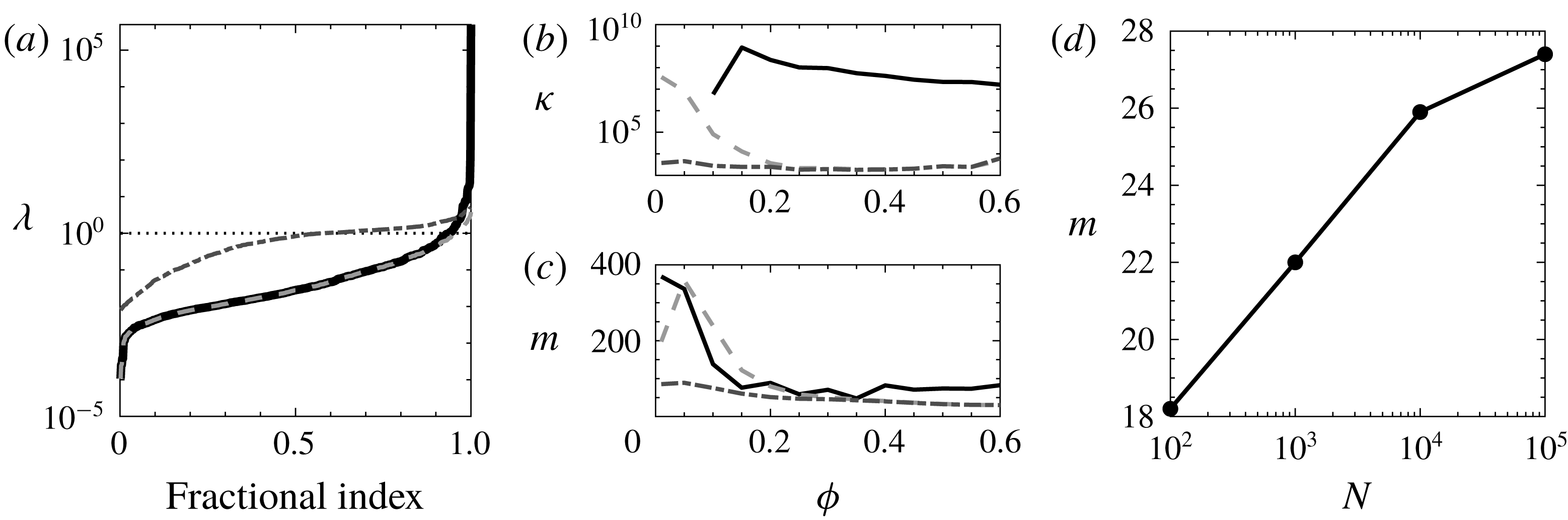
Figure 2(a) shows how these preconditioners compress the spectral radius of the near-field resistance tensor. Specifically, as intended, the incomplete Cholesky factor removes the largest magnitude eigenvalues, while the diagonal preconditioner shifts all eigenvalues that are less than one to be clustered around one. The effect of this eigenspectrum compression on the condition number is shown in figure 2(b) for hard sphere suspensions of 1000 particles across a wide range of volume fractions. The preconditioners produce a well-conditioned operator for all volume fraction and the condition number of the preconditioned operator is independent of
 $\unicode[STIX]{x1D719}$
. Figure 2(c) shows the number of iterations required for the Krylov subspace sampling technique to converge to a step-norm relative error of
 $10^{-6}$
. With our preconditioning scheme, the iteration count is independent of the volume fraction, and is 3–15 times smaller than without preconditioning. Most impressively, figure 2(d) shows that the iteration count is effectively independent of the system size; increasing the number of particles of particles by a factor of 1000 only increases the number of iterations by 50 %.
4.3 Brownian drift
We use the random finite differencing (RFD) scheme of Delong et al. (Reference Delong, Usabiaga, Delgado-Buscalioni, Griffith and Donev2014) to compute the Brownian drift,
 $k_{B}T\unicode[STIX]{x1D735}\boldsymbol{\cdot }\unicode[STIX]{x1D64D}_{FU}$
. This method was already clearly described by Delong et al., but will be summarized here for completeness. The idea of RFD is to approximate the divergence of a matrix
 $\unicode[STIX]{x1D63C}(\boldsymbol{q})$
, which is a function of the set of particle coordinates
 $\boldsymbol{q}$
, as the difference between the matrix evaluated at two nearby points. The central random finite difference is
 $$\begin{eqnarray}\frac{\left\langle \unicode[STIX]{x1D63C}\left(\boldsymbol{q}+{\displaystyle \frac{\unicode[STIX]{x1D716}}{2}}\unicode[STIX]{x0394}\boldsymbol{q}\right)\boldsymbol{\cdot }\unicode[STIX]{x0394}\boldsymbol{q}-\unicode[STIX]{x1D63C}\left(\boldsymbol{q}-{\displaystyle \frac{\unicode[STIX]{x1D716}}{2}}\unicode[STIX]{x0394}\boldsymbol{q}\right)\boldsymbol{\cdot }\unicode[STIX]{x0394}\boldsymbol{q}\right\rangle }{\unicode[STIX]{x1D716}}=\unicode[STIX]{x1D735}\boldsymbol{\cdot }\unicode[STIX]{x1D63C}+O(\unicode[STIX]{x1D716}^{2}),\end{eqnarray}$$
where
 $\unicode[STIX]{x0394}\boldsymbol{q}\sim {\mathcal{N}}(\mathbf{0},\unicode[STIX]{x1D644})$
,
 $\unicode[STIX]{x1D716}$
is a very small discretization parameter, and the finite difference approximates the divergence of
 $\unicode[STIX]{x1D63C}$
in expectation. Methods for choosing
 $\unicode[STIX]{x1D716}$
that maximize the accuracy of the RFD calculation are detailed by Sprinkle et al. (Reference Sprinkle, Balboa Usabiaga, Patankar and Donev2017). This scheme applied to FSD nominally requires two saddle point solves, one at each of the displaced points. However, because the displacements are small, the particle positions are quite close and the solution at one set of coordinates serves as an excellent initial guess for the solution at the other set. The second solve converges very rapidly (
 $O(1)$
iterations are required in our tests, compared to
 $O(10)$
for the first solve), and therefore contributes a negligible amount to the overall computational cost of the algorithm.
Using RFD, the mean drift of the Brownian displacement and stresslet can be computed from saddle point solves,
 $$\begin{eqnarray}\left[\begin{array}{@{}cc@{}}{\mathcal{M}}(\boldsymbol{q}\pm \unicode[STIX]{x0394}\boldsymbol{q}) & \boldsymbol{B}\\ \boldsymbol{B}^{\text{T}} & -\unicode[STIX]{x1D64D}_{FU}^{nf}(\boldsymbol{q}\pm \unicode[STIX]{x0394}\boldsymbol{q})\end{array}\right]\boldsymbol{\cdot }\left[\begin{array}{@{}c@{}}{\mathcal{F}}_{\pm }\\ \boldsymbol{U}_{\pm }\end{array}\right]=\left[\begin{array}{@{}c@{}}\mathbf{0}\\ -\unicode[STIX]{x0394}\boldsymbol{ q}\end{array}\right],\end{eqnarray}$$
where
 ${\mathcal{F}}_{\pm }$
and
 $\boldsymbol{U}_{\pm }$
are the solutions at the positive and negative displacements for the central difference. The far-field hydrodynamic stresslet is
 $\boldsymbol{S}_{\pm }^{ff}=[\mathbf{0}~~\unicode[STIX]{x1D644}]\boldsymbol{\cdot }{\mathcal{F}}_{\pm }$
and the total stresslet is
 $$\begin{eqnarray}\boldsymbol{S}_{\pm }=\boldsymbol{S}_{\pm }^{ff}+\unicode[STIX]{x1D64D}_{SU}^{nf}(\boldsymbol{q}\pm \unicode[STIX]{x0394}\boldsymbol{q})\boldsymbol{\cdot }\boldsymbol{U}_{\pm }.\end{eqnarray}$$
The mean drift of the Brownian displacement is
 $$\begin{eqnarray}\unicode[STIX]{x1D735}\boldsymbol{\cdot }\unicode[STIX]{x1D64D}_{FU}^{-1}=\frac{1}{\unicode[STIX]{x1D716}}\langle \boldsymbol{U}_{+}-\boldsymbol{U}_{-}\rangle +O(\unicode[STIX]{x1D716}^{2}),\end{eqnarray}$$
and the mean drift of the Brownian stresslet is
 $$\begin{eqnarray}-\unicode[STIX]{x1D735}\boldsymbol{\cdot }(\unicode[STIX]{x1D64D}_{SU}\boldsymbol{\cdot }\unicode[STIX]{x1D64D}_{FU}^{-1})=\frac{1}{\unicode[STIX]{x1D716}}\langle \boldsymbol{S}_{+}-\boldsymbol{S}_{-}\rangle +O(\unicode[STIX]{x1D716}^{2}).\end{eqnarray}$$
Transport coefficients for simple cubic lattices as a function of volume fraction. (a) Spin viscosity,
 $\unicode[STIX]{x1D701}$
, computed using the FSD algorithm (circles) compared to ASD results of Sierou & Brady (Reference Sierou and Brady2001) (line). (b) Independent components,
 $\unicode[STIX]{x1D6FC}$
(circles) and
 $\unicode[STIX]{x1D6FD}$
(squares), of the high-frequency shear viscosity,
 $\unicode[STIX]{x1D702}^{S}$
. The solid and dashed lines are the values of
 $\unicode[STIX]{x1D6FC}$
and
 $\unicode[STIX]{x1D6FD}$
, respectively, computed by Brady et al. (Reference Brady, Phillips, Lester and Bossis1988).

5 Results and discussion
5.1 Algorithm validation
A specific implementation of the FSD algorithm for monodisperse spheres is given in appendix B. We validate our FSD algorithm against known static and dynamic results for monodisperse dispersions. Figure 3 shows the spin viscosity and high-frequency shear viscosity of simple cubic lattices of particles. The spin viscosity
 $\boldsymbol{\unicode[STIX]{x1D702}}^{L}$
for a cubic lattice defines the hydrodynamic torque
 $\boldsymbol{L}^{H}$
experienced by the particles as they rotate with angular velocity
 $\unicode[STIX]{x1D734}$
,
 $$\begin{eqnarray}\boldsymbol{L}^{H}=-\boldsymbol{\unicode[STIX]{x1D702}}^{L}\boldsymbol{\cdot }\unicode[STIX]{x1D734}.\end{eqnarray}$$
Because the cubic lattice is isotropic, the spin viscosity can be represented by a single scalar value,
 $$\begin{eqnarray}\unicode[STIX]{x1D702}_{ij}^{L}=\unicode[STIX]{x1D701}\unicode[STIX]{x1D6FF}_{ij}.\end{eqnarray}$$
Similarly, the shear viscosity defines the relationship between the hydrodynamic stresslet
 $\boldsymbol{S}^{H}$
acquired by particles in response to a rate of strain
 $\boldsymbol{E}$
,
 $$\begin{eqnarray}\boldsymbol{S}^{H}=-\boldsymbol{\unicode[STIX]{x1D702}}^{S}\boldsymbol{ : }\boldsymbol{E}.\end{eqnarray}$$
Due to symmetry, the fourth-order tensor
 $\boldsymbol{\unicode[STIX]{x1D702}}^{S}$
describing the shear viscosity can be decomposed in terms of two scalar coefficients (Brady et al.
Reference Brady, Phillips, Lester and Bossis1988),
 $$\begin{eqnarray}\unicode[STIX]{x1D702}_{ijkl}^{S}={\textstyle \frac{1}{2}}(1+\unicode[STIX]{x1D6FD})\left(\unicode[STIX]{x1D6FF}_{ik}\unicode[STIX]{x1D6FF}_{jl}+\unicode[STIX]{x1D6FF}_{il}\unicode[STIX]{x1D6FF}_{jk}-{\textstyle \frac{2}{3}}\unicode[STIX]{x1D6FF}_{ij}\unicode[STIX]{x1D6FF}_{kl}\right)+(\unicode[STIX]{x1D6FC}-\unicode[STIX]{x1D6FD})\left(\unicode[STIX]{x1D6FF}_{ij}\unicode[STIX]{x1D6FF}_{ik}\unicode[STIX]{x1D6FF}_{il}\unicode[STIX]{x1D6FF}_{jk}\unicode[STIX]{x1D6FF}_{jl}\unicode[STIX]{x1D6FF}_{kl}-{\textstyle \frac{1}{3}}\unicode[STIX]{x1D6FF}_{ij}\unicode[STIX]{x1D6FF}_{kl}\right)\!.\end{eqnarray}$$
In general, these viscosity expressions require an ensemble average over all particles, but all particles are identical in a cubic lattice so the averages are omitted here. The scalar coefficients of the spin and shear viscosities were computed using a relative error tolerance of
 $10^{-3}$
in all approximations. The scalar spin viscosity
 $\unicode[STIX]{x1D701}$
is plotted as a function of volume fraction in figure 3(a) and is compared with the values computed by Sierou & Brady (Reference Sierou and Brady2001) using the accelerated Stokesian dynamics (ASD) algorithm. The two scalar components to the shear viscosity,
 $\unicode[STIX]{x1D6FC}$
and
 $\unicode[STIX]{x1D6FD}$
, are plotted as a function of volume fraction in figure 3(b) and are compared with the values obtained by Brady et al. (Reference Brady, Phillips, Lester and Bossis1988) using the original SD algorithm. In all cases, excellent quantitative agreement is observed between our FSD result and the standard Stokesian dynamics approaches.
Equilibrium and transport characteristics for random hard sphere suspensions. (a) Static structure factor for
 $N=1000$
particles computed from dynamic simulations using the FSD algorithm (lines) compared to the analytical Percus–Yevick result for hard spheres (Regnaut & Ravey Reference Regnaut and Ravey1989, Reference Regnaut and Ravey1990). (b) Short-time self-diffusion coefficient computed from the constrained stochastic displacements
 $D_{s}=(\unicode[STIX]{x0394}t/6k_{B}T)\langle \boldsymbol{U}^{B}\boldsymbol{\cdot }\boldsymbol{U}^{B}\rangle$
generated by the FSD algorithm (circles) compared to the analytical results of Ladd (Reference Ladd1990). Error bars represent standard deviations of the measurements.

To validate the proposed sampling and integration methods, we performed dynamic simulations of hard sphere particles with a relative error tolerance of
 $10^{-3}$
for all hydrodynamics calculations and a time step of
 $\unicode[STIX]{x0394}t=10^{-3}$
. To avoid unphysical overlap of the hard sphere particles, we used a short-ranged repulsive potential (Sierou & Brady Reference Sierou and Brady2001). We computed the structure factor of the resulting equilibrium microstructures from 100 configurations extracted from the particle trajectory every 10 bare particle diffusion times. Figure 4(a) shows the structure factor computed from our simulations compared to analytical results derived using the Percus–Yevick closure (Regnaut & Ravey Reference Regnaut and Ravey1989, Reference Regnaut and Ravey1990). The quantitative agreement between our simulations and the analytical theory indicates that the stochastic displacements are consistent with fluctuation–dissipation and produce the correct equilibrium particle configurations. Figure 4(b) shows the short-time self-diffusion coefficient computed from the ensemble mean of the constrained Brownian velocity,
 $\boldsymbol{U}^{B}$
,
 $$\begin{eqnarray}D_{s}=\frac{1}{3}\frac{\unicode[STIX]{x0394}t}{2k_{B}T}\langle \boldsymbol{U}^{B}\boldsymbol{\cdot }\boldsymbol{U}^{B}\rangle ,\end{eqnarray}$$
compared to the high-resolution calculations of Ladd (Reference Ladd1990). Again, quantitative agreement is observed between our calculations and established literature results, indicating that the simulation produces the correct dynamic displacements.
5.2 Algorithm performance
The SD algorithm presented here, which we call fast Stokesian dynamics, is designed for efficient scaling and computations in large system. As detailed in § 4 and appendix B, each component of the FSD algorithm has a computational cost that scales linearly with the number of particles. The most time-consuming calculation is the saddle point inversion because no more effective preconditioners for solution of the stresslet constraint are known. Further acceleration to the algorithm could be achieved by the development of such a preconditioner, should one exist, and would reduce the number of iterations required for the solve. However, the improvement would be modest, as the solution is already evaluated in
 $O(10)$
iterations, as outlined in § 3.3. In this section, we describe the performance characteristics of the FSD algorithm and compare them to our previous work with simpler approximations of the HI.
The expected performance of the FSD algorithm can be estimated from the previously observed performance of our RPY code. This value will serve as a performance baseline. At the RPY level of approximation for the hydrodynamic interactions, the PSE algorithm has a peak performance of around
 $3\times 10^{6}$
particle time steps per second (PTPS) (Fiore et al.
Reference Fiore, Usabiaga, Donev and Swan2017), which is independent of the system size. PTPS is equal to the total number of particles in the simulation divided by the time (in seconds) required to performed a single simulation time step’s worth of calculations. The RPY performance can be used to estimate the optimal performance of the PSE algorithm including lubrication by comparing the operation counts between the two methods. At the RPY level of approximation, there are
 $O(3N)$
degrees of freedom associated with the three independent components of the hydrodynamic force on each particle, and a single matrix-vector multiply is required to evaluate the hydrodynamic interactions. Therefore, computing the RPY approximation for the hydrodynamics requires
 $O(3N)$
operations. In contrast, the FSD approximation includes
 $O(17N)$
degrees of freedom:
 $3N$
from the hydrodynamic force,
 $8N$
from the traceless hydrodynamic couplet, and
 $6N$
from the near-field hydrodynamic force and torque. Additionally, three solves of the saddle point problem need to be evaluated to compute the particle displacements: one solve for the deterministic contribution to particle motion, and two for the RFD approximation to the Brownian drift. However, as previously discussed, the solution of the first RFD solve can be used as the initial guess in the second solve to reduce the second solve to a negligible cost. Therefore, from an operation cost perspective, only two solves are effectively required. Each solve requires approximately 30 iterations regardless of system size, so the total operation count for the FSD algorithm is
 $O(17N\times 30\times 2)=O(1020N)$
, which is 340 times that of the RPY approximation. With this estimate, the expected peak performance of the FSD algorithm is
 $10^{4}$
PTPS.
Performance of the PSE algorithm at three levels of hydrodynamic approximation: RPY (light grey circles), RPY plus stresslets (medium grey squares) and FSD (solid black triangles). Performance of the SEASD algorithm of Wang & Brady (Reference Wang and Brady2016) is shown in open black triangles. The calculations are performed with a relative error tolerance of
 $10^{-3}$
. The performance is measured in particle time steps per second, which is equal to the total number of particles divided by the time required to computed one time steps worth of calculations. The performance of the RPY and RPY+stresslet algorithms is independent of
 $\unicode[STIX]{x1D719}$
, so only one representative curve is shown. Because the FSD performance is a function of
 $\unicode[STIX]{x1D719}$
, the performance for
 $\unicode[STIX]{x1D719}=\{0.1,0.2,0.3,0.4\}$
is computed separately and denoted by the solid, dashed, dashed-dot and dotted lines, respectively.

Figure 5 shows the performance of the PSE algorithm applied to dynamic simulations of hard sphere dispersions performed with a global relative error tolerance of
 $10^{-3}$
, which is typical in many applications (Wang & Brady Reference Wang and Brady2016). Performance curves are shown for the FSD algorithm presented here, as well as for the RPY level of hydrodynamic approximation both with and without the stresslet constraints. In all cases, the computational cost includes the cost of performing the Brownian sampling. The RPY performance, with and without the stresslet constraint, has been previously published and was evaluated on an NVIDIA Tesla K40 graphics card (Fiore et al.
Reference Fiore, Usabiaga, Donev and Swan2017; Fiore & Swan Reference Fiore and Swan2018). The FSD performance presented here was evaluated on an NVIDIA GTX 980Ti graphics card. The GTX has a maximum memory bandwidth of
 $337~\text{GB}~\text{s}^{-1}$
, compared to
 $288~\text{GB}~\text{s}^{-1}$
for the Tesla, and a theoretical maximum performance of 6 teraflops for single precision calculations, compared to 5 teraflops for the Tesla. Whether the application is memory-bound or not, the GTX is expected to be approximately 20 % faster than the Tesla. In our case, we believe the computations are not memory bound. As previously shown, the performance of the RPY stresslet-constrained RPY algorithms is independent of particle volume, so only one curve is plotted for each of these methods.
In contrast to our previous work, the FSD algorithm displays a modest dependence on volume fraction, which is expected based on the convergence rates shown in figure 1(b). As shown in figure 5, there is a factor of 1.3 difference in performance between the
 $\unicode[STIX]{x1D719}=0.1$
and
 $\unicode[STIX]{x1D719}=0.4$
results with
 $N=10^{5}$
. The largest difference between volume fractions is a factor of 3 for
 $N=10^{3}$
. For the largest system sizes studied,
 $N=10^{5}$
, the FSD algorithm is about two times slower than RPY with stresslets. This is substantially better than what would be expected purely from an operation count perspective, even accounting for the difference in maximum theoretical performance between the GPUs. This discrepancy is likely due to the fact that the full computational bandwidth of the GPU is not being used by the RPY or stresslet systems. We have previously noted that the PTPS measured with the RPY algorithm continues to increase up to
 $4\times 10^{6}$
particles (Fiore et al.
Reference Fiore, Usabiaga, Donev and Swan2017), which is evidence of bandwidth underutilization. Furthermore, it is obvious in figure 5 that the throughput of the FSD simulation increases systematically from
 $N=10^{2}$
to
 $N=10^{5}$
, which again indicates that more of the available GPU hardware is being utilized by the larger systems. Additionally, some minor improvements have been made to the far-field algorithms since the method for RPY with stresslet constraints was published, which may contribute slightly to the relative performance differences observed.
Nevertheless, when considered with the performance data for the RPY method, figure 5 clearly demonstrates that the algorithm implementation is optimal and exhibits linear scaling in the total computational complexity with the number of particles modelled. Our algorithm reaches
 $6\times 10^{4}$
PTPS with
 $N=10^{5}$
particles, which for the first time enables such large scale simulations of colloidal materials with full hydrodynamic interactions, including lubrication. This is made plain by comparing the relative performance of our FSD algorithm with the spectral Ewald accelerated Stokesian dynamics (SEASD) algorithm (Wang & Brady Reference Wang and Brady2016), which also leverages GPUs, the non-uniform fast Fourier transform (NUFFT) acceleration of Lindbo & Tornberg (Reference Lindbo and Tornberg2010), and a modestly effective preconditioner for the far-field matrix inversion. The SEASD performance data were obtained for bidisperse suspensions of spheres, for which the performance is expected to be only slightly lower than the monodisperse case considered here. Wang & Brady (Reference Wang and Brady2016) report that their GPU implementation achieves an order of magnitude speedup over an equivalent CPU implementation, which means that the two orders of magnitude difference between FSD and SEASD shown in figure 5 are due primarily, if not exclusively, to the algorithmic improvements presented in this work (Wang & Brady used an NVIDIA GTX 680 GPU, which has a maximum memory bandwidth of
 $192~\text{GB}~\text{s}^{-1}$
and a theoretical maximum performance of 3.25 teraflops for single precision calculations. Therefore, hardware differences amount to at most a factor of 2 difference between their performance and the FSD performance presented here). Specifically, the saddle point hydrodynamic formulation, which avoids nested iterative matrix inversions and for which highly effective preconditioners are developed, and the Brownian force decomposition, which leverages the PSE sampling technique in the far field and a novel preconditioner applied to Krylov subspace techniques in the near field, drastically improve calculation speeds. Furthermore, FSD maintains linear scaling of the computation cost up to
 $10^{5}$
particles, while SEASD performance deteriorates for systems larger than
 $10^{3}$
particles.
6 Stokesian dynamics with arbitrarily shaped particles
The flexibility of the saddle point formulation to incorporate mixed sets of constraints will be illustrated using an important class of hydrodynamic approximations known as composite bead assemblies or rigid multiblobs. In this class of approximation, the surface of an immersed colloidal particle is tessellated with hydrodynamically interacting beads and the motion of the composite particle is computed by solving the resulting immersed boundary problem subject to the constraint that beads belonging to the same particle move together as a rigid body (Balboa Usabiaga et al. Reference Balboa Usabiaga, Kallemov, Delmotte, Bhalla, Griffith and Donev2016; Swan & Wang Reference Swan and Wang2016). This approach is particularly useful for simulating heterogeneous particle mixtures (size and shape polydispersity), and also provides a convergent method to systematically improve the hydrodynamic approximation. The accuracy of the composite bead approximation is improved by increasing the number of beads used to discretize the particle surface, which effectively accounts for higher-order multipole moments (i.e. more non-uniform surface traction) without requiring explicit derivation of the analytical couplings between them.
The composite particles are constructed by discretizing the particle surface using a set of vertices on which hydrodynamically interactions beads are placed. For example, a sphere’s surface can be approximated by a Goldberg polyhedron (Goldberg Reference Goldberg1937), or the surface of a generic shape can be approximated by a triangular mesh. The constraint that beads in the same particle move collectively as a rigid body is enforced by imposing a set of constraint forces
 $\boldsymbol{F}^{c}$
on the beads within each body that act as Lagrange multipliers. The mathematical formulation of the rigid body problem begins with the statement that the constraint forces produce no net force or torque on the composite body of which they are a part, i.e.
 $$\begin{eqnarray}\unicode[STIX]{x1D72E}\boldsymbol{\cdot }\boldsymbol{F}^{c}=\mathbf{0},\end{eqnarray}$$
where
 $\unicode[STIX]{x1D72E}$
is a tensor whose action sums the total force
 $\boldsymbol{F}$
on the beads to produce the resulting generalized force on the composite particle, its adjoint
 $\unicode[STIX]{x1D72E}^{\text{T}}$
computes the bead velocities
 $\boldsymbol{U}$
from the generalized velocity
 $\mathbb{U}$
(translation and rotation) of the rigid body. Including the constraint force, the overdamped force balance on the beads is
 $$\begin{eqnarray}\boldsymbol{F}^{P}+\boldsymbol{F}^{B}+\boldsymbol{F}^{H}+\boldsymbol{F}^{c}=\mathbf{0},\end{eqnarray}$$
where
 $\boldsymbol{F}^{P}$
are the externally imposed conservative forces,
 $\boldsymbol{F}^{B}$
are the set of Brownian forces and
 $\boldsymbol{F}^{H}$
are the hydrodynamic drag forces experienced by the beads. The equivalent force balance on the bodies is obtained by taking the product of
 $\unicode[STIX]{x1D72E}$
with (6.2)
 $$\begin{eqnarray}\mathbb{F}^{P}+\mathbb{F}^{B}+\mathbb{F}^{H}=\mathbf{0},\end{eqnarray}$$
where
 $\mathbb{F}=\unicode[STIX]{x1D72E}\boldsymbol{\cdot }\boldsymbol{F}$
and
 $\mathbb{F}^{c}=\mathbf{0}$
.
In general, each bead interacts hydrodynamically with all other beads according to the mobility relation introduced in § 2,
 ${\mathcal{M}}\boldsymbol{\cdot }{\mathcal{F}}+{\mathcal{B}}\boldsymbol{\cdot }\boldsymbol{U}=\mathbf{0}$
, where
 ${\mathcal{F}}$
is the set of far-field hydrodynamic force moments on the bead (force, torque, stresslet, etc.) and the generalized hydrodynamic force (force and torque) is given by
 $\boldsymbol{F}_{ff}^{H}={\mathcal{B}}^{\text{T}}\boldsymbol{\cdot }{\mathcal{F}}$
. Here,
 ${\mathcal{B}}^{\text{T}}$
projects the generalized force (force and torque) associated with rigid body motion out of the general set of force moments, and its transpose maps rigid body motions onto the higher-order set of considered motions. In the traditional Stokesian dynamics formulation, the hydrodynamic force on the beads is decomposed into near-field and far-field contributions
 $\boldsymbol{F}^{H}=\boldsymbol{F}_{nf}^{H}+\boldsymbol{F}_{ff}^{H}$
. This approach is taken by Meng & Higdon (Reference Meng and Higdon2008a
) to construct platelet-like particles as rigid bead assemblies, but a more general approach decomposes the hydrodynamic force on the particles into a near-field and far-field part,
 $\mathbb{F}^{H}=\mathbb{F}_{nf}^{H}+\mathbb{F}_{ff}^{H}$
, and imposes a specific form for the near-field interactions between particles, not beads. The generic, as yet unspecified, near-field resistance between bodies is denoted
 $\mathbb{R}_{FU}^{nf}$
. In this case, the force balance on the bodies is
 $$\begin{eqnarray}\mathbb{F}^{P}+\mathbb{F}^{B}+\mathbb{F}_{nf}^{H}+\mathbb{F}_{ff}^{H}=\mathbf{0},\end{eqnarray}$$
where
 $$\begin{eqnarray}\mathbb{F}_{nf}^{H}=-\mathbb{R}_{FU}^{nf}\boldsymbol{\cdot }\mathbb{U},\end{eqnarray}$$
and
 $$\begin{eqnarray}\mathbb{F}_{ff}^{H}=\unicode[STIX]{x1D72E}\boldsymbol{\cdot }{\mathcal{B}}^{\text{T}}\boldsymbol{\cdot }{\mathcal{F}}.\end{eqnarray}$$
As in (2.8), the hydrodynamic mobility relation and (6.4)–(6.6) can be combined into a saddle point matrix
 $$\begin{eqnarray}\left[\begin{array}{@{}cc@{}}{\mathcal{M}} & {\mathcal{B}}\boldsymbol{\cdot }\unicode[STIX]{x1D72E}^{\text{T}}\\ \unicode[STIX]{x1D72E}\boldsymbol{\cdot }{\mathcal{B}}^{\text{T}} & -\mathbb{R}_{FU}^{nf}\end{array}\right]\boldsymbol{\cdot }\left[\begin{array}{@{}c@{}}{\mathcal{F}}\\ \mathbb{U}\end{array}\right]=\left[\begin{array}{@{}c@{}}\mathbf{0}\\ -(\mathbb{F}^{P}+\mathbb{F}_{nf}^{B}+\mathbb{F}_{ff}^{B})\end{array}\right].\end{eqnarray}$$
Here,
 $\mathbb{F}_{nf}^{B}$
is the near-field Brownian force,
 $\mathbb{F}_{nf}^{B}\sim {\mathcal{N}}(\mathbf{0},(2k_{B}T/\unicode[STIX]{x0394}t)\mathbb{R}_{FU}^{nf})$
, which can be quickly computed using the techniques described in § 4.2. Equation (6.7) is the specific case of (2.8) applied to composite bead particles. Balboa Usabiaga et al. (Reference Balboa Usabiaga, Kallemov, Delmotte, Bhalla, Griffith and Donev2016) developed a block diagonal preconditioner for fast simulations of so-called rigid multi-blobs, which are equivalent to the rigid bead assemblies considered here. Their preconditioner may be useful to accelerate the solution of (6.7). Meng & Higdon (Reference Meng and Higdon2008b
) compute the Brownian forces for rigid particle assemblies using different techniques for the far-field and near-field forces. The far-field Brownian forces are generated using a second-order rational function approximation, which, while faster than the standard Chebyshev polynomial approximation (Fixman Reference Fixman1986), is also less accurate. The near-field Brownian forces are computed by factorizing
 $\unicode[STIX]{x1D64D}_{FU}^{nf}$
, presumably with a Cholesky factorization, and computing the unconstrained near-field forces using the Cholesky factor, then projecting the resulting forces onto the constrained manifold through the action of
 ${\mathcal{B}}^{\text{T}}$
. In other words, the forces are originally generated on the individual beads comprising each assembly as though the beads were free to move independently, then projected onto the set of allowed rigid body motions. Here we propose a more efficient sampling approach. In the same spirit as (2.20) and the rigid multi-blob work of Balboa Usabiaga et al. (Reference Balboa Usabiaga, Kallemov, Delmotte, Bhalla, Griffith and Donev2016) and Sprinkle et al. (Reference Sprinkle, Balboa Usabiaga, Patankar and Donev2017), the far-field Brownian force can be replaced with a far-field slip velocity
 ${\mathcal{U}}^{B}$
giving
 $\mathbb{F}_{ff}^{B}=\unicode[STIX]{x1D72E}\boldsymbol{\cdot }{\mathcal{B}}^{\text{T}}\boldsymbol{\cdot }{\mathcal{M}}^{-1}\boldsymbol{\cdot }{\mathcal{U}}^{B}$
, so the resulting saddle point equation is
 $$\begin{eqnarray}\left[\begin{array}{@{}cc@{}}{\mathcal{M}} & {\mathcal{B}}\boldsymbol{\cdot }\unicode[STIX]{x1D72E}^{\text{T}}\\ \unicode[STIX]{x1D72E}\boldsymbol{\cdot }{\mathcal{B}}^{\text{T}} & -\mathbb{R}_{FU}^{nf}\end{array}\right]\boldsymbol{\cdot }\left[\begin{array}{@{}c@{}}\hat{{\mathcal{F}}}\\ \mathbb{U}\end{array}\right]=\left[\begin{array}{@{}c@{}}{\mathcal{U}}^{B}\\ -(\mathbb{F}^{P}+\mathbb{F}_{nf}^{B})\end{array}\right],\end{eqnarray}$$
where
 ${\mathcal{U}}^{B}$
is now a Brownian slip velocity on all the beads within the rigid bodies, and can be rapidly generated using the PSE algorithm as summarized in § 4.1, and
 $\hat{{\mathcal{F}}}={\mathcal{F}}+{\mathcal{M}}^{-1}\boldsymbol{\cdot }{\mathcal{U}}^{B}$
.
Schematic illustration for various approximations to the hydrodynamic resistance tensor when using composite bead particles. The bottom row indicates the mathematical representation for the resistance tensor describing the HI between the particles. (a) Individual beads whose interactions are described using the RPY or higher-order multipole expansion for the mobility,
 ${\mathcal{M}}$
. (b) Particles represented using the composite bead model, where each bead propagates flows according to RPY or higher-order multipole approximations. (c) Same as in (b), with an additional near-field interaction between pairs of composite particles is constructed from the sum of the bead–bead near-field interactions between beads in different bodies. (d) Same as in (b), with the near-field interaction between pairs of composite particles represented by coating the particles in lubricating sheets, i.e. body–body near-field interactions rather than bead–bead as in (c).

Equation (6.8) represents a completely general equation for Stokesian dynamics simulations of arbitrarily shaped bodies comprised of rigid bead assemblies. Mixed sizes and shapes are allowed, and only enter the equation through modifications to
 $\unicode[STIX]{x1D72E}$
. In the case where the specific near-field interactions are given by bead–bead lubrication, the near-field resistance tensor is given by
 $\mathbb{R}_{FU}^{nf}=\unicode[STIX]{x1D72E}\boldsymbol{\cdot }\unicode[STIX]{x1D64D}_{FU}^{nf}\boldsymbol{\cdot }\unicode[STIX]{x1D72E}^{\text{T}}$
. The associated Brownian force is computed by generating a random force on each particle,
 $\boldsymbol{F}_{nf}^{B}=(\unicode[STIX]{x1D64D}_{FU}^{nf})^{1/2}\boldsymbol{\cdot }\unicode[STIX]{x1D733}$
, where
 $\unicode[STIX]{x1D733}\sim {\mathcal{N}}(\mathbf{0},(2k_{B}T/\unicode[STIX]{x0394}t)\unicode[STIX]{x1D644})$
, then projecting that set of forces onto the constrained set of forces consistent with rigid body motion,
 $\mathbb{F}_{nf}^{B}=\unicode[STIX]{x1D72E}\boldsymbol{\cdot }(\unicode[STIX]{x1D64D}_{FU}^{nf})^{1/2}\boldsymbol{\cdot }\unicode[STIX]{x1D733}$
. Figure 6 provides an illustration of the various approximations to the hydrodynamics of spherical particles using the techniques summarized here.
An important distinction between the physical meaning of the beads used in the general approach advocated here and the more specific approach taken by Meng & Higdon (Reference Meng and Higdon2008a
) bears additional discussion and illuminates some advantages of the proposed method. In the approach taken by Meng & Higdon (Reference Meng and Higdon2008a
), each bead is treated as a rigid object with lubricating interactions, i.e. the stresslet constraint associated with rigid motion is solved for each bead. In other words, the composite particles are meant to literally model assemblies of rigid spherical particles; one can think of gluing hard spheres together to achieve a desired shape. This may not be the desired hydrodynamic model in more general circumstances. A schematic illustration of different composite bead approaches is shown in figure 6. A simpler computational method can be developed by noting that the flow field around a rigid particle can be expressed solely in terms of a single layer potential (Kim & Karrila Reference Kim and Karrila2005). This means that the force dipole (torque and stresslet) on the beads (but not on the particles) is irrelevant to the particle dynamics and can be neglected, and the beads can be allowed to interact with one another through the simple RPY approximation. This approach has been previously demonstrated by Swan & Wang (Reference Swan and Wang2016) and Balboa Usabiaga et al. (Reference Balboa Usabiaga, Kallemov, Delmotte, Bhalla, Griffith and Donev2016). In this way, each bead can be thought of as a regularized point force, and the collection of beads within each particle an approximation to the non-uniform force distribution on its surface. Adding lubrication between particles (not beads) improves the effective resolution of the force distribution without resorting to finer discretization. In the results presented in this section, we use this simpler approach and set
 ${\mathcal{M}}={\mathcal{M}}_{RPY}$
everywhere. Using the RPY approximation includes the additional simplification that
 ${\mathcal{B}}=\unicode[STIX]{x1D644}$
. The rigid body constraint implicity captures dipoles, quadrupoles, and higher-order multipole force moments by producing a non-uniform distribution of hydrodynamic bead forces on each particle. Sequential resolution of higher-order moments is achieved by increasing the number of beads used to discretize each particle. This approach has an added benefit of reducing the algorithm’s computational cost. With the force dipole and lubrication interactions considered at the bead–bead level, there are 17 degrees of freedom per bead, or
 $17\,N_{b}\,N_{p}$
total degrees of freedom, where
 $N_{b}$
is the number of beads per particle and
 $N_{p}$
is the total number of particles. When only RPY interactions are considered between beads, and lubrication interactions are considered between particles, there are only 3 degrees of freedom per bead and 6 per particle, i.e.
 $(3N_{b}+6)N_{p}$
in total. Therefore, the speedup expected by using particle–particle lubrication is
 $17N_{b}/(3N_{b}+6)\approx 17/3$
for modestly large
 $N_{b}$
(
 $N_{b}\gtrsim 10$
), which are typical in many simulations.
Next, the rigid body construction with body–body near-field lubrication interactions (figure 6 d) will be combined with the stochastic sampling schemes described in § 4 to produce accurate and physically consistent simulations. The effect of increasing resolution and adding lubrication on the convergence of the hydrodynamic approximation is also illustrated.
Some minor modifications to the near-field calculation described in § 3 are required here and are detailed for clarity. In the traditional Stokesian dynamics approach, the lubrication interactions are computed by
 $$\begin{eqnarray}\unicode[STIX]{x1D64D}_{2B}^{nf}=\unicode[STIX]{x1D64D}_{2B}-{\mathcal{R}}_{2B},\end{eqnarray}$$
where
 $\unicode[STIX]{x1D64D}_{2B}^{nf}$
is the pair contribution to the near-field resistance tensor,
 $\unicode[STIX]{x1D64D}_{2B}$
is the exact lubrication expression for a pair of spherical particles, typically computed using the expressions given by Jeffrey & Onishi (Reference Jeffrey and Onishi1984), and
 ${\mathcal{R}}_{2B}$
is the far-field contribution to the pair resistance tensor. When the particles are represented in the far field by a collection of RPY beads, the lubrication tensor between two composite bead assemblies is built by
 $$\begin{eqnarray}\mathbb{R}_{2B}^{nf}=\unicode[STIX]{x1D64D}_{2B}-\unicode[STIX]{x1D72E}_{2B}\boldsymbol{\cdot }{\mathcal{M}}_{2B}^{-1}\boldsymbol{\cdot }\unicode[STIX]{x1D72E}_{2B}^{\text{T}},\end{eqnarray}$$
where
 ${\mathcal{M}}_{2B}$
is the mobility tensor for the beads comprising both rigid bodies and
 $\unicode[STIX]{x1D72E}_{2B}$
contains the rigid body tensor for the two bodies in the pair, and the radii used in the expressions for
 $\unicode[STIX]{x1D64D}_{2B}$
are the hydrodynamic radius of the composite particle. For spherical particles, it is obvious that the hydrodynamic radius corresponds to the effective radius computed from the translational diffusivity (Swan & Wang Reference Swan and Wang2016), but for other shapes the relevant length scale is less clear. In other words, the far-field contribution to the pair resistance tensor is computed by solving the hydrodynamic rigid body problem for that particle pair. It is necessary to choose approximations for the tensors in (6.10) that result in a positive semi-definite matrix. For particles with a finite radius of curvature, there will always be a cutoff distance within which the lubrication interactions dominate the far-field interactions and a positive-definite
 $\mathbb{R}_{2B}^{nf}$
is guaranteed.
The PSE technique is used to generate the far-field slip velocity in (6.8) and the preconditioned near-field sampling scheme described in § 4 is used to sample
 $\mathbb{F}_{nf}^{B}$
from
 $\mathbb{R}^{nf}$
. Finally, random finite differences, which have previously been successfully applied to Brownian dynamics simulations of rigid bodies (Delong, Balboa Usabiaga & Donev Reference Delong, Balboa Usabiaga and Donev2015), are used to compute the Brownian drift and are combined with an Euler–Maruyama integration scheme. While previous efforts have developed RFD-free integration schemes to implicitly account for the thermal drift in pure mobility (Delmotte & Keaveny Reference Delmotte and Keaveny2015; Sprinkle et al.
Reference Sprinkle, Balboa Usabiaga, Patankar and Donev2017; Fiore & Swan Reference Fiore and Swan2018) and resistance (Banchio & Brady Reference Banchio and Brady2003) problems, it is substantially more challenging to develop such integrators for the mixed problem considered here, where the near-field stochastic quantity is a force and far-field stochastic quantity is a velocity. This representation of the noise is necessary for performance but not easily reconciled with the RFD-free methods.
A simple test of the proposed integration scheme is to connect two particles with a spring potential,
 $U(r)$
, which varies with the interparticle separation, then compute the distribution of the observed centre-to-centre distance
 $r$
between the particles. This is a useful test because the Boltzmann distribution provides an analytical result for the equilibrium probability density of the centre-to-centre distance
 $f(r)$
,
 $$\begin{eqnarray}f(r)=C_{f}r^{2}\text{e}^{-U(r)/k_{B}T},\end{eqnarray}$$
where the probability of a given state
 $i$
with energy
 $U_{i}$
is
 $\text{e}^{-U_{i}/k_{B}T}$
and the number of available states at a given distance
 $r$
is proportional to
 $r^{2}$
. The constant
 $C_{f}$
ensures that the total probability density integrates to one,
 $C_{f}=\int _{0}^{\infty }\text{d}rr^{2}\text{e}^{-U(r)/k_{B}T}$
. The associated cumulative distribution function,
 $F(r)$
, is defined as
 $$\begin{eqnarray}F(r)=\int _{0}^{r}\text{d}xf(x).\end{eqnarray}$$
These distributions were computed for a pair of particles, each comprised of 12 beads, interacting via a constant force spring for which
 $U(r)/k_{B}T=k|r-r_{0}|$
(with the parameters
 $k=2.5$
and
 $r_{0}=3a$
) by integrating their trajectories over 100 bare particle diffusion times. The results are shown in figure 7 and agree quantitatively with the analytical results in (6.11) and (6.12). If fluctuation–dissipation were not satisfied or if the thermal drift were incorrectly computed, then the equilibrium distribution would not be obtained and the distributions presented in figure 7, and would have noticeable error in either the variance or mean. The fact that the simulated distributions are correct indicate that the decomposition of the HI into near-field and far-field contributions and the associated decomposed stochastic sampling techniques produces stochastic displacements that are consistent with the fluctuation–dissipation theorem, and which correctly account for the thermal drift.
Probability functions (symbols) for the centre-to-centre distance of two particles connected by a linear spring with spring constant
 $k/k_{B}T=2.5$
and equilibrium separation
 $r_{0}=3a$
compared to the theoretical Boltzmann distribution (lines). Circles and crosses represent calculations with and without the thermal drift included, respectively. (a) Probability density function. (b) Cumulative distribution function. A short-ranged repulsive interaction is added to prevent particle overlap.

The distributions presented in figure 6 only test the equilibrium statistics of the stochastic integration scheme, and therefore do not probe the effect of bead resolution or lubrication on the dynamics. Increasing the number of beads used to tesselate a particle’s surface improves the approximation to the hydrodynamic interactions and increases the hydrodynamic resistance, especially between nearly touching particles. The lubrication corrections introduced in Stokesian dynamics also improve the approximation because they are designed to precisely capture the pair contribution to those near-field interactions. Therefore, by including lubrication with the composite bead approach, it would be expected that the number of tessellating beads required to represent the HI at a given level of accuracy would be lower than if the lubrication terms were not included. To quantify this effect, we computed the eigenspectrum of the constrained mobility tensor for spherical particles,
 $\mathbb{R}^{-1}$
(whose action is inferred by solving the saddle point problem for rigid body motion, equation (6.8)), at various levels of surface discretization, i.e. different numbers of beads per particle
 $N_{b}$
, both with and without the near-field particle–particle lubrication interactions.
Distribution of eigenvalues of the constrained mobility tensor,
 $\mathbb{R}_{FU}^{-1}$
, computed from the constrained saddle point solution, for composite bead particles with (lines) and without (symbols) particle–particle lubrication interactions. Particles are represented by composite beads comprised of
 $N_{B}=12,41,162$
beads, denoted by black, dark grey and light grey, respectively. Two types of configurations are used, both comprised of
 $N=27$
particles at
 $\unicode[STIX]{x1D719}=0.9\unicode[STIX]{x03C0}/6$
: (a) simple cubic crystal and (b) random hard sphere fluid.

Figure 8(a) shows the eigenspectrum of
 $\mathbb{R}_{FU}^{-1}$
, computed from the constrained saddle point solve, for a periodic simple cubic lattice comprised of 27 particles per unit cell at a volume fraction of
 $\unicode[STIX]{x1D719}=(0.9)\unicode[STIX]{x03C0}/6$
, where
 $\unicode[STIX]{x1D719}=\unicode[STIX]{x03C0}/6$
is the closest-packing volume fraction for the simple cubic lattice. Because the surface of each particle is approximated by a discrete set of beads, a secondary lattice comprised of the beads is superimposed over the lattice comprised of the particle centres of mass and is unavoidable. To minimize the effect of this secondary lattice on the calculation, each composite particle is rotated randomly about its centre of mass so that the bead coordinates on any two particles are uncorrelated. For perfectly spherical particles, the eigenvalues exist at discrete levels due to lattice symmetry. The secondary bead lattice effects causes these discrete levels to smear out, a phenomena which is most noticeable at coarse discretizations, particularly
 $N_{b}=12$
. When particle–particle lubrication is neglected, increasing
 $N_{b}$
shifts the eigenspectra down to smaller eigenvalues. When lubrication is accounted for, the eigenspectra for all resolutions collapse onto a single curve. The exception is with the eigenvalues whose indices are above 140, which do not collapse to the same value for different resolutions even when lubrication is added. These eigenvalues are associated with sedimentation modes of the lattice, for which it is known that pairwise lubrication does not improve calculation accuracy because there is no relative motion between particles sedimenting in a lattice. For all modes except the sedimentation mode, a simple 12-bead surface discretization with particle–particle lubrication interactions is more accurate than a 162-bead surface tesselation without lubrication. The effect of discretization on transport properties computed in suspensions of adhesive hard spheres has been considered previously in some specific applications (Fiore, Wang & Swan Reference Fiore, Wang and Swan2018; Wang, Fiore & Swan Reference Wang, Fiore and Swan2019), but a general and systematic study of suspension transport properties computed using composite bead assemblies appears to be absent from the literature.
Part of the dramatic collapse of the eigenspectra with pair lubrication is due to the symmetry of the simple cubic lattice. For a random hard sphere fluid with the same number of particles and volume fraction, shown in figure 8(b), it’s clear that adding the pairwise lubrication approximation does substantially improve results even at low-order surface discretizations, but the collapse of all the spectra with the addition of lubrication that was observed for the crystal is no longer seen, and improvements in accuracy are still made by increasing
 $N_{b}$
. Without the symmetry of the lattice, high-order many-body interactions need to be resolved to compute the full dynamic spectrum. The only way to achieve this using the composite bead method is to increase the particle resolution. Resolving the many-body effect of lubricating flows, for example using the method proposed by Lefebvre-Lepot, Merlet & Nguyen (Reference Lefebvre-Lepot, Merlet and Nguyen2015), might lead to the same eigenspectra collapse as was observed in the lattice, enabling very high fidelity simulations at small
 $N_{b}$
. (The random hard sphere fluid configuration used in the calculation is included in the supplementary material, available at https://doi.org/10.1017/jfm.2019.640, so that eigenspectra computed using various methods can be directly compared.) Nevertheless, and importantly for fast simulations, the pairwise lubrication approximation qualitatively captures the diminutive eigenvalues associated with very nearly touching particles even for low-resolution discretizations. Without lubrication, many surface elements are needed to resolve these eigenvalues, therefore including particle–particle lubrication dramatically improves the simulation accuracy for a marginal increase in computational cost. As demonstrated in §§ 3.3 and 4.2, the total computational cost of the proposed simulation method with Brownian dynamics is linear in the total number of hydrodynamic objects, in this case beads. As each bead has three associated degrees of freedom the simulation cost without lubrication is
 $O(3N_{p}N_{b})$
for
 $N_{p}$
total particles. Introducing particle–particle lubrication increases the cost to
 $O((3N_{b}+6)N_{p})$
because lubrication adds six degrees of freedom per particle. At the lowest bead resolutions used here,
 $N_{b}=12$
, the simulation cost without lubrication is
 $O(36N_{p})$
and
 $O(42N_{p})$
with it. The 12-bead model with lubrication produces results that are qualitatively similar to the 162-bead model without lubrication, for which the cost is
 $O(486N_{p})$
. The results in figure 8(b), combined with these simple estimates, show that a 12-bead model with particle–particle lubrication maintains quantitatively similar dynamics to the 162-bead model, but is an order of magnitude faster to compute.
7 Conclusion
Our recently developed PSE algorithm for rapid Brownian dynamics simulations with HI represented at the RPY levels of approximations with stresslet constraints has been extended to incorporate the near-field lubrication correction required for Stokesian dynamics. The hydrodynamic approximation is reformulated in a generic saddle point matrix, which encompasses many existing hydrodynamic approximations for colloidal particles. Critically, the saddle point formulation obviates the need to solve a resistance problem, i.e. invert the hydrodynamic mobility tensor, which is an ill-conditioned problem. Combined with efficient preconditioners based on the Schur complement of the hydrodynamic saddle point matrix, the saddle point matrix solve exhibits a linear computational complexity in the total number of particles modelled. We have also shown that the stochastic Brownian force, which is traditionally decomposed into near-field and far-field contributions, is more effectively computed when decomposed into the sum of a near-field force and a far-field slip velocity. The slip velocity can be readily computed using fast techniques such as the PSE algorithm and the near-field Brownian force is computed with a preconditioned Krylov subspace approximation for the square root of the resistance tensor containing the near-field lubrication interactions of all particles. The preconditioner used for this scheme can be recycled from the saddle point solve. In contrast to the standard approach for Stokesian dynamics with Brownian forces, this approach is readily parallelizable and is therefore extensible to large systems. The resulting algorithm, which we call fast Stokesian dynamics (FSD), has linear overall computational complexity and is nearly as fast as the RPY algorithm with stresslet constraints. The speed of the algorithm enables dynamics simulations of
 $O(10^{5})$
particles in reasonable wall times on a single consumer-grade GPU.
We believe that the saddle point formulation presented here is a very general representation for constrained problems in colloidal hydrodynamics. This formulation is especially powerful because it enables the pairing of arbitrary near-field and far-field HI approximations with a general procedure for generating stochastic velocities consistent with a given set of constraints.
Acknowledgements
J.W.S. and A.M.F. gratefully acknowledge funding from the MIT Energy Initiative Shell Seed Fund and NSF Career Award CBET-1554398.
Supplementary material
Supplementary material is available at https://doi.org/10.1017/jfm.2019.640.
Appendix A. Polydispersity in Rotne–Prager-like models of hydrodynamics in dispersions of spherical particles
For polydisperse suspensions the effect of differing sizes on the hydrodynamic interactions can be included directly in the far-field mobility shape factor and the near-field resistance tensor expressions. The near-field lubrication series can be used without modification because the formulae given by Jeffrey & Onishi (Reference Jeffrey and Onishi1984) and Jeffrey (Reference Jeffrey1992b ) are already defined for unequal particle size ratios.
The far-field mobility couplings modified to account for polydispersity begin with the Fourier-space representation for the pair mobility coupling between two particles of unequal sizes
 $a$
and
 $b$
is
 $$\begin{eqnarray}\unicode[STIX]{x1D648}_{pq}^{\unicode[STIX]{x1D6FC}\unicode[STIX]{x1D6FD}}=\frac{1}{\unicode[STIX]{x1D702}V}\mathop{\sum }_{\boldsymbol{k}\neq \mathbf{0}}\text{e}^{\text{i}\boldsymbol{k}\boldsymbol{\cdot }(\boldsymbol{x}_{\unicode[STIX]{x1D6FC}}-\boldsymbol{x}_{\unicode[STIX]{x1D6FD}})}\frac{1}{k^{2}}\boldsymbol{s}^{p}(ka)(\unicode[STIX]{x1D644}-\hat{\boldsymbol{k}}\hat{\boldsymbol{k}})\boldsymbol{s}^{q}(kb).\end{eqnarray}$$
The different sizes enter the problem through the shape factors,
 $\boldsymbol{s}$
. After applying Hasimoto’s splitting function, the real-space and wave-space contributions are given by
 $$\begin{eqnarray}\displaystyle & \displaystyle (\unicode[STIX]{x1D648}_{pq}^{\unicode[STIX]{x1D6FC}\unicode[STIX]{x1D6FD}})_{r}=\frac{1}{\unicode[STIX]{x1D702}V}\mathop{\sum }_{\boldsymbol{k}\neq \mathbf{0}}\text{e}^{\text{i}\boldsymbol{k}\boldsymbol{\cdot }(\boldsymbol{x}_{\unicode[STIX]{x1D6FC}}-\boldsymbol{x}_{\unicode[STIX]{x1D6FD}})}\frac{1}{k^{2}}(1-H(k,\unicode[STIX]{x1D709}))\boldsymbol{s}^{p}(ka)(\unicode[STIX]{x1D644}-\hat{\boldsymbol{k}}\hat{\boldsymbol{k}})\boldsymbol{s}^{q}(kb), & \displaystyle\end{eqnarray}$$
 $$\begin{eqnarray}\displaystyle & \displaystyle (\unicode[STIX]{x1D648}_{pq}^{\unicode[STIX]{x1D6FC}\unicode[STIX]{x1D6FD}})_{w}=\frac{1}{\unicode[STIX]{x1D702}V}\mathop{\sum }_{\boldsymbol{k}\neq \mathbf{0}}\text{e}^{\text{i}\boldsymbol{k}\boldsymbol{\cdot }(\boldsymbol{x}_{\unicode[STIX]{x1D6FC}}-\boldsymbol{x}_{\unicode[STIX]{x1D6FD}})}\frac{1}{k^{2}}H(k,\unicode[STIX]{x1D709})\boldsymbol{s}^{p}(ka)(\unicode[STIX]{x1D644}-\hat{\boldsymbol{k}}\hat{\boldsymbol{k}})\boldsymbol{s}^{q}(kb). & \displaystyle\end{eqnarray}$$
A.1 Real-space sum
As before, the real-space terms are expressed as the product of scalar functions of distance, and now particle sizes, and a minimal set of tensors, derived using appropriate symmetry and tracelessness conditions. The scalar coefficients are computed by analytically evaluating the integral corresponding to the inverse Fourier transform in (A 2). The integration can be split into two parts: an integral over the solid angle and an integral over the wavenumber. The solid angle integrals give the tensorial structure of each mobility relation and are straightforward to compute because they only involve exponentials and trigonometric functions. The wavenumber integral is much more challenging to compute and results in the complicated closed form expressions given previously for monodisperse suspensions (Fiore & Swan Reference Fiore and Swan2018). Although the expressions are valid for all particle separations, the integrals are simpler to evaluate, and the resulting expressions are more numerically stable, if the integrals are evaluated independently for each of five cases,
 $$\begin{eqnarray}\displaystyle & r\geqslant a+b, & \displaystyle\end{eqnarray}$$
 $$\begin{eqnarray}\displaystyle & a-b<b-a<r<a+b, & \displaystyle\end{eqnarray}$$
 $$\begin{eqnarray}\displaystyle & 0<a-b<r<b-a, & \displaystyle\end{eqnarray}$$
 $$\begin{eqnarray}\displaystyle & 0<b-a<r<a-b, & \displaystyle\end{eqnarray}$$
 $$\begin{eqnarray}\displaystyle & 0=r. & \displaystyle\end{eqnarray}$$
These cases correspond to widely separated particles, partially overlapping particles, and the smaller particle enveloped by the larger particle. All the integrals presented below produce scalar mobility functions that are of the form
 $$\begin{eqnarray}\displaystyle f^{(i)} & = & \displaystyle f_{0}^{(i)}+f_{1}^{(i)}\text{e}^{-(a+b+r)^{2}\unicode[STIX]{x1D709}^{2}}+f_{2}^{(i)}\text{e}^{-(a+b-r)^{2}\unicode[STIX]{x1D709}^{2}}+f_{3}^{(i)}\text{e}^{-(-a+b+r)^{2}\unicode[STIX]{x1D709}^{2}}\nonumber\\ \displaystyle & & \displaystyle +\,f_{4}^{(i)}\text{e}^{-(a-b+r)^{2}\unicode[STIX]{x1D709}^{2}}+f_{5}^{(i)}\,\text{erfc}((-a-b+r)\unicode[STIX]{x1D709})+f_{6}^{(i)}\,\text{erfc}((a-b+r)\unicode[STIX]{x1D709})\nonumber\\ \displaystyle & & \displaystyle +\,f_{7}^{(i)}\,\text{erfc}((-a+b+r)\unicode[STIX]{x1D709})+f_{8}^{(i)}\,\text{erfc}((a+b+r)\unicode[STIX]{x1D709}).\end{eqnarray}$$
The functions
 $f_{j}^{(i)}$
are various combinations of products, sums, differences, and quotients of
 $a$
,
 $b$
,
 $\unicode[STIX]{x1D709}$
and
 $r$
, and various powers thereof. Their tabulation would take many pages and are omitted here for brevity, but are included in the supplementary material. In the following sections, we show how to construct the integrals from which these coefficients can be computed.
A.1.1 Translation-force coupling
The pair mobility tensor for the translation-force coupling is a function only of the unit vector between the two particle centres,
 $\hat{\boldsymbol{r}}$
, the magnitude of the particle centre-to-centre separation,
 $r$
, the radii of the two particles,
 $a$
and
 $b$
, and the Ewald splitting parameter
 $\unicode[STIX]{x1D709}$
. The translation-force coupling,
 $\unicode[STIX]{x1D648}_{UF}$
is a rank-2 tensor and is constructed in a minimal form as the sum of two orthogonal basis sets,
 $$\begin{eqnarray}\unicode[STIX]{x1D614}_{ij}^{UF}=f_{1}(r,a,b,\unicode[STIX]{x1D709})(\unicode[STIX]{x1D6FF}_{ij}-\hat{r}_{i}\hat{r}_{j})+f_{2}(r,a,b,\unicode[STIX]{x1D709})\hat{r}_{i}\hat{r}_{j}.\end{eqnarray}$$
The scalar functions
 $f_{1}$
and
 $f_{2}$
are computed by evaluating the tensor products with the integral corresponding to the inverse Fourier transform of the wave-space representation for the real-space contribution to the Ewald sum of
 $\unicode[STIX]{x1D614}_{ij}^{UF}$
. This representation is
 $$\begin{eqnarray}\unicode[STIX]{x1D614}_{ij}^{UF}=-\frac{1}{\unicode[STIX]{x1D707}V}\mathop{\sum }_{\boldsymbol{q}\neq \mathbf{0}}\text{e}^{\text{i}\boldsymbol{q}\boldsymbol{\cdot }\boldsymbol{r}}\unicode[STIX]{x1D614}_{q}^{UF}(\unicode[STIX]{x1D6FF}_{ij}-\hat{q}_{i}\hat{q}_{j}),\end{eqnarray}$$
where
 $$\begin{eqnarray}\unicode[STIX]{x1D614}_{q}^{UF}=\frac{1}{q^{2}}\text{j}_{0}(qa)\text{j}_{0}(qb)H(q\unicode[STIX]{x1D709}^{-1})\end{eqnarray}$$
is the scale factor at wavenumber
 $q$
,
 $\text{j}_{m}$
is the
 $m$
th order spherical Bessel function of the first kind and
 $H(x)=1-(1+x^{2}/4)\text{e}^{-x^{2}/4}$
.
The first integral is the inverse Fourier transform of
 $\unicode[STIX]{x1D614}_{ij}^{UF}(\unicode[STIX]{x1D6FF}_{ij}-\hat{r}_{i}\hat{r}_{j})$
, and its evaluation will be used to illustrate how the more complicated integrals later in this appendix are performed,
 $$\begin{eqnarray}\displaystyle f_{1} & = & \displaystyle -\frac{1}{\unicode[STIX]{x1D707}V}\mathop{\sum }_{\boldsymbol{q}\neq \mathbf{0}}\text{e}^{\text{i}\boldsymbol{q}\boldsymbol{\cdot }\boldsymbol{r}}\unicode[STIX]{x1D614}_{q}^{UF}(\unicode[STIX]{x1D6FF}_{ij}-\hat{q}_{i}\hat{q}_{j})(\unicode[STIX]{x1D6FF}_{ij}-\hat{r}_{i}\hat{r}_{j}),\nonumber\\ \displaystyle & = & \displaystyle -\frac{1}{\unicode[STIX]{x1D707}V}\mathop{\sum }_{\boldsymbol{q}\neq \mathbf{0}}\text{e}^{\text{i}\boldsymbol{q}\boldsymbol{\cdot }\boldsymbol{r}}\unicode[STIX]{x1D614}_{q}^{UF}(\unicode[STIX]{x1D6FF}_{ij}\unicode[STIX]{x1D6FF}_{ij}-\unicode[STIX]{x1D6FF}_{ij}\hat{q}_{i}\hat{q}_{j}-\unicode[STIX]{x1D6FF}_{ij}\hat{r}_{i}\hat{r}_{j}+\hat{q}_{i}\hat{q}_{j}\hat{r}_{i}\hat{r}_{j}),\nonumber\\ \displaystyle & = & \displaystyle -\frac{1}{(2\unicode[STIX]{x03C0})^{3}\unicode[STIX]{x1D707}}\int \text{d}\boldsymbol{q}\text{e}^{\text{i}\boldsymbol{q}\boldsymbol{\cdot }\boldsymbol{r}}\unicode[STIX]{x1D614}_{q}^{UF}(\unicode[STIX]{x1D6FF}_{ij}\unicode[STIX]{x1D6FF}_{ij}-\unicode[STIX]{x1D6FF}_{ij}\hat{q}_{i}\hat{q}_{j}-\unicode[STIX]{x1D6FF}_{ij}\hat{r}_{i}\hat{r}_{j}+\hat{q}_{i}\hat{q}_{j}\hat{r}_{i}\hat{r}_{j}).\end{eqnarray}$$
To evaluate these tensor products, the distance vector
 $\hat{\boldsymbol{r}}$
can be aligned along the
 $z$
-axis in the spherical coordinates of integration, so that
 $\hat{\boldsymbol{q}}\boldsymbol{\cdot }\hat{\boldsymbol{r}}=\cos \unicode[STIX]{x1D703}$
, where
 $\unicode[STIX]{x1D703}$
is the polar angle,
 $$\begin{eqnarray}\displaystyle f_{1} & = & \displaystyle -\frac{1}{(2\unicode[STIX]{x03C0})^{3}\unicode[STIX]{x1D707}}\int \text{d}\boldsymbol{q}\text{e}^{\text{i}qr\cos \unicode[STIX]{x1D703}}\unicode[STIX]{x1D614}_{q}^{UF}(1+\cos ^{2}\unicode[STIX]{x1D703}),\nonumber\\ \displaystyle & = & \displaystyle -\frac{1}{(2\unicode[STIX]{x03C0})^{3}\unicode[STIX]{x1D707}}\int \text{d}qq^{2}\unicode[STIX]{x1D614}_{q}^{UF}\int _{\unicode[STIX]{x1D6FA}}\text{d}\unicode[STIX]{x1D6FA}\text{e}^{\text{i}qr\cos \unicode[STIX]{x1D703}}(1+\cos ^{2}\unicode[STIX]{x1D703}),\end{eqnarray}$$
where
 $\unicode[STIX]{x1D6FA}$
represents the integral over the solid angle,
 $\int _{\unicode[STIX]{x1D6FA}}\text{d}\unicode[STIX]{x1D6FA}=\int _{0}^{\unicode[STIX]{x03C0}}\text{d}\unicode[STIX]{x1D703}\sin \unicode[STIX]{x1D703}\int _{0}^{2\unicode[STIX]{x03C0}}\text{d}\unicode[STIX]{x1D719}$
. Because none of the parameters depend on the azimuthal angle,
 $\unicode[STIX]{x1D719}$
, that integral only contributions a multiplicative factor of
 $2\unicode[STIX]{x03C0}$
so that
 $$\begin{eqnarray}f_{1}=-\frac{1}{(2\unicode[STIX]{x03C0})^{2}\unicode[STIX]{x1D707}}\int \text{d}qq^{2}\unicode[STIX]{x1D614}_{q}^{UF}\int _{0}^{\unicode[STIX]{x03C0}}\text{d}\unicode[STIX]{x1D703}\sin \unicode[STIX]{x1D703}(1+\cos ^{2}\unicode[STIX]{x1D703})\text{e}^{\text{i}qr\cos \unicode[STIX]{x1D703}}.\end{eqnarray}$$
The second integral is the inverse Fourier transform of
 $\unicode[STIX]{x1D614}_{ij}^{UF}\,\hat{r}_{i}\hat{r}_{j}$
 $$\begin{eqnarray}\displaystyle f_{2} & = & \displaystyle -\frac{1}{\unicode[STIX]{x1D707}V}\mathop{\sum }_{\boldsymbol{q}\neq \mathbf{0}}\text{e}^{\text{i}\boldsymbol{q}\boldsymbol{\cdot }\boldsymbol{r}}\unicode[STIX]{x1D614}_{q}^{UF}(\unicode[STIX]{x1D6FF}_{ij}-\hat{q}_{i}\hat{q}_{j})\hat{r}_{i}\hat{r}_{j},\nonumber\\ \displaystyle & = & \displaystyle -\frac{1}{(2\unicode[STIX]{x03C0})^{3}\unicode[STIX]{x1D707}}\int \text{d}qq^{2}\unicode[STIX]{x1D614}_{q}^{UF}\int _{\unicode[STIX]{x1D6FA}}\text{d}\unicode[STIX]{x1D6FA}\text{e}^{\text{i}qr\cos \unicode[STIX]{x1D703}}(1-\cos ^{2}\unicode[STIX]{x1D703}),\nonumber\\ \displaystyle & = & \displaystyle -\frac{1}{(2\unicode[STIX]{x03C0})^{2}\unicode[STIX]{x1D707}}\int \text{d}qq^{2}\unicode[STIX]{x1D614}_{q}^{UF}\int _{0}^{\unicode[STIX]{x03C0}}\text{d}\unicode[STIX]{x1D703}\sin ^{3}\unicode[STIX]{x1D703}\text{e}^{\text{i}qr\cos \unicode[STIX]{x1D703}}.\end{eqnarray}$$
A.1.2 Minimal tensor representation of translation-dipole coupling
The translation-dipole coupling can be written using two scalar mobility functions,
 $$\begin{eqnarray}\unicode[STIX]{x1D614}_{imn}^{UC}=g_{1}(\unicode[STIX]{x1D6FF}_{im}\hat{r}_{n}-\hat{r}_{i}\hat{r}_{m}\hat{r}_{n})+g_{2}(\unicode[STIX]{x1D6FF}_{in}\hat{r}_{m}+\unicode[STIX]{x1D6FF}_{mn}\hat{r}_{i}-4\hat{r}_{i}\hat{r}_{m}\hat{r}_{n}).\end{eqnarray}$$
From a general expression for
 $\unicode[STIX]{x1D614}_{imn}^{UC}$
, the scalar functions
 $g_{1}$
and
 $g_{2}$
can be isolated by evaluating the inner product of the mobility tensor with the appropriate orthogonal tensors. The products of
 $\unicode[STIX]{x1D614}_{imn}^{UC}$
with these tensors are
 $$\begin{eqnarray}\displaystyle & \unicode[STIX]{x1D614}_{imn}^{UC}\hat{r}_{i}\hat{r}_{m}\hat{r}_{n}=-2g_{2} & \displaystyle\end{eqnarray}$$
 $$\begin{eqnarray}\displaystyle & \unicode[STIX]{x1D614}_{imn}^{UC}(\unicode[STIX]{x1D6FF}_{im}-\hat{r}_{i}\hat{r}_{m})\hat{r}_{n}=2g_{1}. & \displaystyle\end{eqnarray}$$
The coefficients
 $g_{1}$
and
 $g_{2}$
will be determined by evaluating the independent integral corresponding to the inverse Fourier transform of the wave-space representation of real-space contribution to
 $\unicode[STIX]{x1D614}_{imn}^{UC}$
.
The wave-space representation of the real-space contribution to the Ewald sum of
 $\unicode[STIX]{x1D614}_{imn}^{UC}$
is
 $$\begin{eqnarray}\unicode[STIX]{x1D614}_{imn}^{UC}=-\frac{1}{\unicode[STIX]{x1D707}V}\mathop{\sum }_{\boldsymbol{q}\neq \mathbf{0}}\text{e}^{\text{i}\boldsymbol{q}\boldsymbol{\cdot }\boldsymbol{r}}\unicode[STIX]{x1D614}_{q}^{UC}(\unicode[STIX]{x1D6FF}_{im}-\hat{q}_{i}\hat{q}_{m})\hat{q}_{n},\end{eqnarray}$$
where
 $$\begin{eqnarray}\unicode[STIX]{x1D614}_{q}^{UC}=\frac{1}{q^{2}}\text{j}_{0}(qa)\left(\frac{3\text{i}}{b}\text{j}_{1}(qb)\right)H(q\unicode[STIX]{x1D709}^{-1})\end{eqnarray}$$
is the scale factor at wavenumber
 $q$
.
The integral for
 $g_{1}$
is the inverse Fourier transform of
 $\unicode[STIX]{x1D614}_{imn}^{UC}(\unicode[STIX]{x1D6FF}_{im}-\hat{r}_{i}\hat{r}_{m})\hat{r}_{n}$
 $$\begin{eqnarray}\displaystyle g_{1} & = & \displaystyle -\frac{1}{2}\frac{1}{\unicode[STIX]{x1D707}V}\mathop{\sum }_{\boldsymbol{q}\neq \mathbf{0}}\text{e}^{\text{i}\boldsymbol{q}\boldsymbol{\cdot }\boldsymbol{r}}\unicode[STIX]{x1D614}_{q}^{UC}(\unicode[STIX]{x1D6FF}_{im}-\hat{q}_{i}\hat{q}_{m})\hat{q}_{n}(\unicode[STIX]{x1D6FF}_{im}-\hat{r}_{i}\hat{r}_{m})\hat{r}_{n},\nonumber\\ \displaystyle & = & \displaystyle -\frac{1}{2}\frac{(2\unicode[STIX]{x03C0})^{-3}}{\unicode[STIX]{x1D707}}\int _{0}^{\infty }\text{d}qq^{2}\int _{\unicode[STIX]{x1D6FA}}\text{d}\unicode[STIX]{x1D6FA}\text{e}^{\text{i}\boldsymbol{q}\boldsymbol{\cdot }\boldsymbol{r}}\unicode[STIX]{x1D614}_{q}^{UC}(1+\cos ^{2}\unicode[STIX]{x1D703})\cos \unicode[STIX]{x1D703},\nonumber\\ \displaystyle & = & \displaystyle -\frac{1}{2}\frac{(2\unicode[STIX]{x03C0})^{-2}}{\unicode[STIX]{x1D707}}\int _{0}^{\infty }\text{d}qq^{2}\unicode[STIX]{x1D614}_{q}^{UC}\int _{0}^{\unicode[STIX]{x03C0}}\text{d}\unicode[STIX]{x1D703}\sin \unicode[STIX]{x1D703}(1+\cos ^{2}\unicode[STIX]{x1D703})\cos \unicode[STIX]{x1D703}\text{e}^{\text{i}qr\cos \unicode[STIX]{x1D703}}.\end{eqnarray}$$
The integral for
 $g_{2}$
is the inverse Fourier transform of
 $\unicode[STIX]{x1D614}_{imn}^{UC}\hat{r}_{i}\hat{r}_{m}\hat{r}_{n}$
 $$\begin{eqnarray}\displaystyle g_{2} & = & \displaystyle \frac{1}{2}\frac{1}{\unicode[STIX]{x1D707}V}\mathop{\sum }_{\boldsymbol{q}\neq \mathbf{0}}\text{e}^{\text{i}\boldsymbol{q}\boldsymbol{\cdot }\boldsymbol{r}}\unicode[STIX]{x1D614}_{q}^{UC}(\unicode[STIX]{x1D6FF}_{im}-\hat{q}_{i}\hat{q}_{m})\hat{q}_{n}\hat{r}_{i}\hat{r}_{m}\hat{r}_{n}\nonumber\\ \displaystyle & = & \displaystyle \frac{1}{2}\frac{(2\unicode[STIX]{x03C0})^{-2}}{\unicode[STIX]{x1D707}}\int _{0}^{\infty }\text{d}qq^{2}\unicode[STIX]{x1D614}_{q}^{UC}\int _{0}^{\unicode[STIX]{x03C0}}\text{d}\unicode[STIX]{x1D703}\sin ^{3}\unicode[STIX]{x1D703}\cos \unicode[STIX]{x1D703}\text{e}^{\text{i}qr\cos \unicode[STIX]{x1D703}}.\end{eqnarray}$$
Note that the gradient-force coupling for particle pair
 $\unicode[STIX]{x1D6FC},\unicode[STIX]{x1D6FD}$
can be obtained from the velocity-dipole coupling through symmetry relations, i.e.
 $\unicode[STIX]{x1D614}_{imn}^{UC}(\unicode[STIX]{x1D6FC},\unicode[STIX]{x1D6FD})=\unicode[STIX]{x1D614}_{nmi}^{DF}(\unicode[STIX]{x1D6FD},\unicode[STIX]{x1D6FC})$
.
A.1.3 Minimal tensor representation of gradient-dipole coupling
The pair mobility tensor for the gradient-dipole coupling can be written using three scalar mobility functions,
 $$\begin{eqnarray}\displaystyle \unicode[STIX]{x1D614}_{ijkl}^{DC} & = & \displaystyle h_{1}(\unicode[STIX]{x1D6FF}_{ij}\unicode[STIX]{x1D6FF}_{kl}+\unicode[STIX]{x1D6FF}_{ik}\unicode[STIX]{x1D6FF}_{jl}-4\unicode[STIX]{x1D6FF}_{il}\unicode[STIX]{x1D6FF}_{jk})+h_{2}(\unicode[STIX]{x1D6FF}_{jk}\hat{r}_{i}\hat{r}_{l}-\hat{r}_{i}\hat{r}_{j}\hat{r}_{k}\hat{r}_{l})\nonumber\\ \displaystyle & & \displaystyle +\,h_{3}(\unicode[STIX]{x1D6FF}_{ij}\hat{r}_{k}\hat{r}_{l}+\unicode[STIX]{x1D6FF}_{ik}\hat{r}_{j}\hat{r}_{l}+\unicode[STIX]{x1D6FF}_{jl}\hat{r}_{i}\hat{r}_{k}+\unicode[STIX]{x1D6FF}_{kl}\hat{r}_{i}\hat{r}_{j}+\unicode[STIX]{x1D6FF}_{il}\hat{r}_{j}\hat{r}_{k}-6\hat{r}_{i}\hat{r}_{j}\hat{r}_{k}\hat{r}_{l}-\unicode[STIX]{x1D6FF}_{il}\unicode[STIX]{x1D6FF}_{jk}).\qquad\end{eqnarray}$$
Where the variables have been renamed for simplicity, as there are now only three scalar functions to be determined. A full-rank set of linear combinations of the scalar functions can be isolated by the appropriate tensor inner products,
 $$\begin{eqnarray}\displaystyle & \unicode[STIX]{x1D614}_{ijkl}^{DC}\hat{r}_{i}\hat{r}_{j}\hat{r}_{k}\hat{r}_{l}=-2h_{1}-2h_{3}, & \displaystyle\end{eqnarray}$$
 $$\begin{eqnarray}\displaystyle & \unicode[STIX]{x1D614}_{ijkl}^{DC}\unicode[STIX]{x1D6FF}_{il}\hat{r}_{j}\hat{r}_{k}=-10h_{1}-2h_{3}, & \displaystyle\end{eqnarray}$$
 $$\begin{eqnarray}\displaystyle & \unicode[STIX]{x1D614}_{ijkl}^{DC}\unicode[STIX]{x1D6FF}_{jk}\hat{r}_{i}\hat{r}_{l}=-10h_{1}+2h_{2}-4h_{3}. & \displaystyle\end{eqnarray}$$
Now there is a linear combination of integrals required to separate each scalar function, so a linear system must be solved. The linear system is
 $$\begin{eqnarray}\left[\begin{array}{@{}c@{}}\unicode[STIX]{x1D614}_{ijkl}^{DC}\hat{r}_{i}\hat{r}_{j}\hat{r}_{k}\hat{r}_{l}\\ \unicode[STIX]{x1D614}_{ijkl}^{DC}\unicode[STIX]{x1D6FF}_{il}\hat{r}_{j}\hat{r}_{k}\\ \unicode[STIX]{x1D614}_{ijkl}^{DC}\unicode[STIX]{x1D6FF}_{jk}\hat{r}_{i}\hat{r}_{l}\end{array}\right]=\left[\begin{array}{@{}ccc@{}}-2 & 0 & -2\\ -10 & 0 & -2\\ -10 & 2 & -4\end{array}\right]\left[\begin{array}{@{}c@{}}h_{1}\\ h_{2}\\ h_{3}\end{array}\right],\end{eqnarray}$$
and the inverse is
 $$\begin{eqnarray}\left[\begin{array}{@{}c@{}}h_{1}\\ h_{2}\\ h_{3}\end{array}\right]=\frac{1}{8}\left[\begin{array}{@{}ccc@{}}1 & -1 & 0\\ -5 & -3 & 1\\ -5 & 1 & 0\end{array}\right]\left[\begin{array}{@{}c@{}}\unicode[STIX]{x1D614}_{ijkl}^{DC}\hat{r}_{i}\hat{r}_{j}\hat{r}_{k}\hat{r}_{l}\\ \unicode[STIX]{x1D614}_{ijkl}^{DC}\unicode[STIX]{x1D6FF}_{il}\hat{r}_{j}\hat{r}_{k}\\ \unicode[STIX]{x1D614}_{ijkl}^{DC}\unicode[STIX]{x1D6FF}_{jk}\hat{r}_{i}\hat{r}_{l}\end{array}\right].\end{eqnarray}$$
The coefficients
 $h_{1}$
,
 $h_{2}$
and
 $h_{3}$
are therefore given by linear combinations of these tensor products with the integral corresponding to the inverse Fourier transform of the wave-space representation of the real-space contribution to
 $\unicode[STIX]{x1D614}_{ijkl}^{DC}$
.
The wave-space representation of the real-space contribution to the Ewald sum of
 $\unicode[STIX]{x1D614}_{ijkl}^{DC}$
is
 $$\begin{eqnarray}\unicode[STIX]{x1D614}_{ijkl}^{DC}=-\frac{1}{\unicode[STIX]{x1D707}V}\mathop{\sum }_{\boldsymbol{q}\neq \mathbf{0}}\text{e}^{\text{i}\boldsymbol{q}\boldsymbol{\cdot }\boldsymbol{r}}\unicode[STIX]{x1D614}_{q}^{DC}\hat{q}_{i}(\unicode[STIX]{x1D6FF}_{jk}-\hat{q}_{j}\hat{q}_{k})\hat{q}_{l},\end{eqnarray}$$
where
 $$\begin{eqnarray}\unicode[STIX]{x1D614}_{q}^{DC}=\frac{1}{q^{2}}\left(\frac{3\sqrt{-1}}{a}\text{j}_{1}(qa)\right)\left(\frac{3\sqrt{-1}}{b}\text{j}_{1}(qb)\right)H(q\unicode[STIX]{x1D709}^{-1})\end{eqnarray}$$
is the scale factor at wavenumber
 $q$
, and
 $\text{j}_{m}$
is the
 $m$
th-order spherical Bessel function of the first kind and
 $H(x)=1-(1+x^{2}/4)\text{e}^{-x^{2}/4}$
is Hasimoto’s splitting function.
The first integral is the inverse Fourier transform
 $$\begin{eqnarray}\displaystyle \unicode[STIX]{x1D614}_{ijkl}^{DC}\hat{r}_{i}\hat{r}_{j}\hat{r}_{k}\hat{r}_{l} & = & \displaystyle -\frac{1}{\unicode[STIX]{x1D707}V}\mathop{\sum }_{\boldsymbol{q}\neq \mathbf{0}}\text{e}^{\text{i}\boldsymbol{q}\boldsymbol{\cdot }\boldsymbol{r}}\unicode[STIX]{x1D614}_{q}^{DC}\hat{q}_{i}(\unicode[STIX]{x1D6FF}_{jk}-\hat{q}_{j}\hat{q}_{k})\hat{q}_{l}\hat{r}_{i}\hat{r}_{j}\hat{r}_{k}\hat{r}_{l}\nonumber\\ \displaystyle & = & \displaystyle -\frac{1}{\unicode[STIX]{x1D707}V}\mathop{\sum }_{\boldsymbol{q}\neq \mathbf{0}}\text{e}^{\text{i}\boldsymbol{q}\boldsymbol{\cdot }\boldsymbol{r}}\unicode[STIX]{x1D614}_{q}^{DC}\sin ^{2}\unicode[STIX]{x1D703}\cos ^{2}\unicode[STIX]{x1D703}\nonumber\\ \displaystyle & = & \displaystyle -\frac{(2\unicode[STIX]{x03C0})^{-3}}{\unicode[STIX]{x1D707}}\int _{0}^{\infty }\text{d}qq^{2}\int _{\unicode[STIX]{x1D6FA}}\text{d}\unicode[STIX]{x1D6FA}\text{e}^{\text{i}\boldsymbol{q}\boldsymbol{\cdot }\boldsymbol{r}}\unicode[STIX]{x1D614}_{q}^{DC}\sin ^{2}\unicode[STIX]{x1D703}\cos ^{2}\unicode[STIX]{x1D703}\nonumber\\ \displaystyle & = & \displaystyle -\frac{(2\unicode[STIX]{x03C0})^{-2}}{\unicode[STIX]{x1D707}}\int _{0}^{\infty }\text{d}qq^{2}\unicode[STIX]{x1D614}_{q}^{DC}\int _{0}^{\unicode[STIX]{x03C0}}\text{d}\unicode[STIX]{x1D703}\sin ^{3}\unicode[STIX]{x1D703}\cos ^{2}\unicode[STIX]{x1D703}\text{e}^{\text{i}qr\cos \unicode[STIX]{x1D703}}.\end{eqnarray}$$
The second integral is the inverse Fourier transform
 $$\begin{eqnarray}\displaystyle \unicode[STIX]{x1D614}_{ijkl}^{DC}\unicode[STIX]{x1D6FF}_{il}\hat{r}_{j}\hat{r}_{k} & = & \displaystyle -\frac{1}{\unicode[STIX]{x1D707}V}\mathop{\sum }_{\boldsymbol{q}\neq \mathbf{0}}\text{e}^{\text{i}\boldsymbol{q}\boldsymbol{\cdot }\boldsymbol{r}}\unicode[STIX]{x1D614}_{q}^{DC}\hat{q}_{i}(\unicode[STIX]{x1D6FF}_{jk}-\hat{k}_{j}\hat{k}_{k})\hat{q}_{l}\unicode[STIX]{x1D6FF}_{il}\hat{r}_{j}\hat{r}_{k}\nonumber\\ \displaystyle & = & \displaystyle -\frac{(2\unicode[STIX]{x03C0})^{-2}}{\unicode[STIX]{x1D707}}\int _{0}^{\infty }\text{d}qq^{2}\unicode[STIX]{x1D614}_{q}^{DC}\int _{0}^{\unicode[STIX]{x03C0}}\text{d}\unicode[STIX]{x1D703}\sin ^{3}\unicode[STIX]{x1D703}\text{e}^{\text{i}qr\cos \unicode[STIX]{x1D703}}.\end{eqnarray}$$
The third integral is the inverse Fourier transform
 $$\begin{eqnarray}\displaystyle \unicode[STIX]{x1D614}_{ijkl}^{DC}\unicode[STIX]{x1D6FF}_{jk}\hat{r}_{i}\hat{r}_{l} & = & \displaystyle -\frac{1}{\unicode[STIX]{x1D707}V}\mathop{\sum }_{\boldsymbol{q}\neq \mathbf{0}}\text{e}^{\text{i}\boldsymbol{q}\boldsymbol{\cdot }\boldsymbol{r}}\unicode[STIX]{x1D614}_{q}^{DC}\hat{q}_{i}(\unicode[STIX]{x1D6FF}_{jk}-\hat{q}_{j}\hat{q}_{k})\hat{q}_{l}\unicode[STIX]{x1D6FF}_{jk}\hat{r}_{i}\hat{r}_{l}\nonumber\\ \displaystyle & = & \displaystyle -2\frac{(2\unicode[STIX]{x03C0})^{-2}}{\unicode[STIX]{x1D707}}\int _{0}^{\infty }\text{d}qq^{2}\unicode[STIX]{x1D614}_{q}^{DC}\int _{0}^{\unicode[STIX]{x03C0}}\text{d}\unicode[STIX]{x1D703}\sin \unicode[STIX]{x1D703}\cos ^{2}\unicode[STIX]{x1D703}\text{e}^{\text{i}qr\cos \unicode[STIX]{x1D703}}.\end{eqnarray}$$
The analytical expressions resulting from evaluating these integrals can be found using symbolic integration packages such as Mathematica, but the resulting expressions are very sensitive at very small values of
 $r$
and
 $\unicode[STIX]{x1D709}$
. Specifically, errors in floating point arithmetic come into play and destabilize the result. In this case, asymptotic expressions at small
 $\unicode[STIX]{x1D709}$
can be derived and used instead. For general purpose use, quadruple precision arithmetic can minimize the floating point arithmetic error when evaluating the algebraic expressions resulting from the preceding integrals, and single or double precision can be used to tabulate them for use in fast simulations.
A.2 Wave-space sum
The wave-space sum could be computed using the non-uniform discrete Fourier transform (NUDFT), however the associated cost would be
 $O(N^{2})$
. To use the accelerated NUFFT, we have to derive quadrature operations that account for the differing finite sizes. Following the approach of Lindbo & Tornberg (Reference Lindbo and Tornberg2010), and using the shape factors in (A 1), we can define kernels that map particle forces and couplets onto the fluid force density,
 $\boldsymbol{H}$
, and whose adjoints map the impinging velocity field,
 $\tilde{\boldsymbol{H}}$
onto particle velocities and velocity gradients. The math is straightforward and the result is that for finite size particles, the force is spread onto the gridded force density according to
 $$\begin{eqnarray}H_{i}(\,\boldsymbol{y})=\mathop{\sum }_{\unicode[STIX]{x1D6FD}}F_{i}^{\unicode[STIX]{x1D6FD}}\left(\frac{2\unicode[STIX]{x1D709}^{2}}{\unicode[STIX]{x03C0}\unicode[STIX]{x1D707}}\right)^{3/2}\text{e}^{-2\unicode[STIX]{x1D709}^{2}r^{2}/\unicode[STIX]{x1D707}}K_{1}(r,b),\end{eqnarray}$$
and the couplet is similarly spread by
 $$\begin{eqnarray}H_{i}(\,\boldsymbol{y})=\mathop{\sum }_{\unicode[STIX]{x1D6FD}}C_{ip}^{\unicode[STIX]{x1D6FD}}r_{p}\left(\frac{2\unicode[STIX]{x1D709}^{2}}{\unicode[STIX]{x03C0}\unicode[STIX]{x1D707}}\right)^{3/2}\text{e}^{-2\unicode[STIX]{x1D709}^{2}r^{2}/\unicode[STIX]{x1D707}}K_{2}(r,b),\end{eqnarray}$$
where the sum is over all particles,
 $\boldsymbol{y}$
is a point in the fluid, and
 $\boldsymbol{r}=\boldsymbol{y}-\boldsymbol{x}_{\unicode[STIX]{x1D6FD}}$
is the minimum image distance between the particle centre
 $\boldsymbol{x}_{\unicode[STIX]{x1D6FD}}$
and the fluid point
 $\boldsymbol{y}$
. The parameter
 $\unicode[STIX]{x1D707}$
was introduced by Lindbo & Tornberg (Reference Lindbo and Tornberg2010) to control the resolution of the NUFFT kernels on the underlying grid representing the fluid. (Lindbo & Tornberg used
 $\unicode[STIX]{x1D702}$
to denote this parameter, but we use
 $\unicode[STIX]{x1D707}$
here to avoid confusion with the fluid viscosity, which has been represented by
 $\unicode[STIX]{x1D702}$
throughout this work.) The adjoint contraction/interpolation operators are similarly
 $$\begin{eqnarray}(U_{i}^{\unicode[STIX]{x1D6FC}})_{w}=\frac{1}{\unicode[STIX]{x1D707}}\int _{\unicode[STIX]{x1D6FA}}\text{d}\boldsymbol{y}\tilde{H}_{i}(\,\boldsymbol{y})\left(\frac{2\unicode[STIX]{x1D709}^{2}}{\unicode[STIX]{x03C0}\unicode[STIX]{x1D707}}\right)^{3/2}\text{e}^{-2\unicode[STIX]{x1D709}^{2}r^{2}/\unicode[STIX]{x1D707}}K_{1}(r,a)\end{eqnarray}$$
and
 $$\begin{eqnarray}(\unicode[STIX]{x1D60B}_{ij}^{\unicode[STIX]{x1D6FC}})_{w}=\frac{1}{\unicode[STIX]{x1D707}}\int _{\unicode[STIX]{x1D6FA}}\text{d}\boldsymbol{y}\tilde{H}_{i}(\,\boldsymbol{y})r_{j}\left(\frac{2\unicode[STIX]{x1D709}^{2}}{\unicode[STIX]{x03C0}\unicode[STIX]{x1D707}}\right)^{3/2}\text{e}^{-2\unicode[STIX]{x1D709}^{2}r^{2}/\unicode[STIX]{x1D707}}K_{2}(r,a).\end{eqnarray}$$
Here,
 $K_{1}$
and
 $K_{2}$
are the kernels that define how the first and second force and velocity moments are mapped to and from the fluid force and velocity field,
 $$\begin{eqnarray}\displaystyle & \displaystyle K_{1}(r,b)=\left(\text{e}^{-2\unicode[STIX]{x1D709}^{2}b^{2}/\unicode[STIX]{x1D707}}\frac{\sinh (4\unicode[STIX]{x1D709}^{2}br/\unicode[STIX]{x1D707})}{4\unicode[STIX]{x1D709}^{2}br/\unicode[STIX]{x1D707}}\right), & \displaystyle\end{eqnarray}$$
 $$\begin{eqnarray}\displaystyle & \displaystyle K_{2}(r,b)=3\left(\text{e}^{-2\unicode[STIX]{x1D709}^{2}b^{2}/\unicode[STIX]{x1D707}}\frac{\sinh (4\unicode[STIX]{x1D709}^{2}br/\unicode[STIX]{x1D707})-(4\unicode[STIX]{x1D709}^{2}br/\unicode[STIX]{x1D707})\cosh (4\unicode[STIX]{x1D709}^{2}br/\unicode[STIX]{x1D707})}{(4\unicode[STIX]{x1D709}^{2}br/\unicode[STIX]{x1D707})^{3}}\right). & \displaystyle\end{eqnarray}$$
Note that this is the exact same result as obtained by Lindbo & Tornberg (Reference Lindbo and Tornberg2010) modified by an effective shape factor accounting for the way the finite size distributes the force moment. Physically, the point (Gaussian) kernels of Lindbo & Tornberg distribute forces about the centre of each particle, whereas the finite size kernels presented here distribute forces around the edges. This fact is more apparent when the summand in (A 35) is rewritten using the kernel from (A 39) and rearranged using the definition of
 $\sinh$
,
 $$\begin{eqnarray}F_{i}^{\unicode[STIX]{x1D6FD}}\left(\frac{2\unicode[STIX]{x1D709}^{2}}{\unicode[STIX]{x03C0}\unicode[STIX]{x1D707}}\right)^{3/2}\left(\frac{1}{8\unicode[STIX]{x1D709}^{2}br/\unicode[STIX]{x1D707}}\right)(\text{e}^{-2\unicode[STIX]{x1D709}^{2}(r-b)^{2}/\unicode[STIX]{x1D707}}-\text{e}^{-2\unicode[STIX]{x1D709}^{2}(r+b)^{2}/\unicode[STIX]{x1D707}}).\end{eqnarray}$$
We can follow the approach of Lindbo & Tornberg (Reference Lindbo and Tornberg2010) to derive bounds for the quadrature error associated with the modified kernels in (A 37) and (A 38). Bounds will be derived only for the kernel in (A 39) because it decays the most slowly with
 $r$
, so the error associated with kernels of higher order moments will be contained by the same bound.
The quadrature approximation to the integral in (A 37) is
 $$\begin{eqnarray}\boldsymbol{Q}=h^{3}\mathop{\sum }_{\boldsymbol{n}=-P/2}^{P/2}\tilde{\boldsymbol{H}}(\boldsymbol{n}h)K(\boldsymbol{n}h,a),\end{eqnarray}$$
where
 $h$
is the grid spacing,
 $h^{3}$
is the volume of a grid element,
 $P$
is the number of grid points within the support of each particle in each direction and
 $K(\boldsymbol{r},b)=(2\unicode[STIX]{x1D709}^{2}/\unicode[STIX]{x03C0}\unicode[STIX]{x1D707})^{3/2}\text{e}^{-2\unicode[STIX]{x1D709}^{2}r^{2}/\unicode[STIX]{x1D707}}K_{1}(r,b)$
. It is understood that in the sum each element of
 $\boldsymbol{n}$
goes from
 $-P/2$
to
 $P/2$
. The error associated with this quadrature approximation is
 $$\begin{eqnarray}\unicode[STIX]{x1D716}_{q}=\left\Vert \boldsymbol{Q}-\int _{\unicode[STIX]{x1D6FA}}\text{d}\boldsymbol{y}\tilde{\boldsymbol{H}}(\,\boldsymbol{y})K(\,\boldsymbol{y},a)\right\Vert ,\end{eqnarray}$$
which is most conveniently evaluated by splitting into two pieces and applying the triangle inequality
 $$\begin{eqnarray}\unicode[STIX]{x1D716}_{q}\leqslant \left\Vert h^{3}\mathop{\sum }_{\Vert \boldsymbol{n}\Vert _{\infty }\leqslant P/2}\tilde{\boldsymbol{H}}(\boldsymbol{n}h)K(\boldsymbol{n}h)-\int _{\unicode[STIX]{x1D6FA}}\text{d}\boldsymbol{y}\tilde{\boldsymbol{H}}(\,\boldsymbol{y})K(\,\boldsymbol{y})\right\Vert +\left\Vert h^{3}\mathop{\sum }_{\Vert \boldsymbol{n}\Vert _{\infty }>P/2}\tilde{\boldsymbol{H}}(\boldsymbol{n}h)K(\boldsymbol{n}h)\right\Vert .\end{eqnarray}$$
The two terms in this equation,
 $$\begin{eqnarray}\displaystyle & \displaystyle A=\left\Vert h^{3}\mathop{\sum }_{n\leqslant P/2}\tilde{\boldsymbol{H}}(\boldsymbol{n}h)K(\boldsymbol{n}h)-\int _{\unicode[STIX]{x1D6FA}}\text{d}\boldsymbol{y}\tilde{\boldsymbol{H}}(\,\boldsymbol{y})K(\,\boldsymbol{y})\right\Vert , & \displaystyle\end{eqnarray}$$
 $$\begin{eqnarray}\displaystyle & \displaystyle B=\left\Vert h^{3}\mathop{\sum }_{n>P/2}\tilde{\boldsymbol{H}}(\boldsymbol{n}h)K(\boldsymbol{n}h)\right\Vert , & \displaystyle\end{eqnarray}$$
are bound using two different approaches.
To derive a bound on the value of
 $A$
, we start with Poisson’s summation formula,
 $h^{3}\sum _{\boldsymbol{n}}\boldsymbol{f}(\boldsymbol{n}h)=\sum _{\boldsymbol{k}}\hat{\boldsymbol{f}}(\boldsymbol{k}/h)$
, where
 $\boldsymbol{f}=\tilde{\boldsymbol{H}}K$
,
 $$\begin{eqnarray}A=\left\Vert \mathop{\sum }_{\boldsymbol{k}}\hat{\boldsymbol{f}}(\boldsymbol{k}/h)-\int _{\unicode[STIX]{x1D6FA}}\text{d}\boldsymbol{y}\tilde{\boldsymbol{H}}(\,\boldsymbol{y})K(\,\boldsymbol{y})\right\Vert .\end{eqnarray}$$
By the definition of the Fourier transform,
 $\hat{\boldsymbol{f}}(\boldsymbol{k})=\int _{\unicode[STIX]{x1D6FA}}\text{d}\boldsymbol{y}\text{e}^{-\text{i}\boldsymbol{k}\boldsymbol{\cdot }\boldsymbol{y}}\boldsymbol{f}(\,\boldsymbol{y})$
, it is obvious that
 $\hat{\boldsymbol{f}}(\mathbf{0})=\int _{\unicode[STIX]{x1D6FA}}\text{d}\boldsymbol{y}\tilde{\boldsymbol{H}}(\,\boldsymbol{y})K(\,\boldsymbol{y})$
so that:
 $$\begin{eqnarray}A=\left\Vert \mathop{\sum }_{|k|>0}\hat{\boldsymbol{f}}(\boldsymbol{k}/h)\right\Vert .\end{eqnarray}$$
Here,
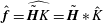 $\hat{\boldsymbol{f}}=\widehat{\tilde{\boldsymbol{H}}K}=\tilde{\boldsymbol{H}}\ast \hat{K}$
is a quantity that decays at least as quickly as
 $\hat{K}$
with increasing
 $|k|$
because
 $\tilde{\boldsymbol{H}}$
is an approximately uniform quantity. Therefore
 $$\begin{eqnarray}A\leqslant C_{A}\left\Vert \mathop{\sum }_{|k|>0}\hat{K}(\boldsymbol{k}/h)\right\Vert =C_{A}\left\Vert \mathop{\sum }_{|k|>0}\frac{\sin (ka/h)}{ka/h}\text{e}^{-\unicode[STIX]{x1D707}k^{2}/8\unicode[STIX]{x1D709}^{2}h^{2}}\right\Vert .\end{eqnarray}$$
Noting that
 $\Vert \text{sin}\,(ka/h)/(ka/h)\Vert \leqslant 1$
,
 $$\begin{eqnarray}A\leqslant C_{A}\left\Vert \mathop{\sum }_{|k|>0}\text{e}^{-\unicode[STIX]{x1D707}k^{2}/8\unicode[STIX]{x1D709}^{2}h^{2}}\right\Vert .\end{eqnarray}$$
Replacing the non-integer wavevector
 $k$
with the integer wavenumber
 $\unicode[STIX]{x1D705}$
,
 $k=2\unicode[STIX]{x03C0}\unicode[STIX]{x1D705}$
, allows the sum to be evaluated explicitly,
 $$\begin{eqnarray}\mathop{\sum }_{\unicode[STIX]{x1D705}=1}^{\infty }\text{e}^{-\unicode[STIX]{x03C0}^{2}\unicode[STIX]{x1D707}\unicode[STIX]{x1D705}^{2}/2\unicode[STIX]{x1D709}^{2}h^{2}}={\textstyle \frac{1}{2}}(\unicode[STIX]{x1D717}_{3}(0,\text{e}^{-\unicode[STIX]{x03C0}^{2}\unicode[STIX]{x1D707}/2\unicode[STIX]{x1D709}^{2}h^{2}})-1)\leqslant c\text{e}^{-\unicode[STIX]{x03C0}^{2}\unicode[STIX]{x1D707}/2\unicode[STIX]{x1D709}^{2}h^{2}},\end{eqnarray}$$
where
 $\unicode[STIX]{x1D717}_{a}(x,q)$
is the elliptic (Jacobi) theta function and
 $c$
is an unspecified constant. Therefore,
 $$\begin{eqnarray}A\leqslant C_{A}^{\prime }\text{e}^{-\unicode[STIX]{x03C0}^{2}\unicode[STIX]{x1D707}/2\unicode[STIX]{x1D709}^{2}h^{2}}.\end{eqnarray}$$
The value of
 $B$
is bound by the integral
 $$\begin{eqnarray}B=\left\Vert h^{3}\mathop{\sum }_{|\boldsymbol{n}|>P/2}\tilde{\boldsymbol{H}}(\boldsymbol{n}h)K(\boldsymbol{n}h)\right\Vert \leqslant \int _{hP/2}^{\infty }\text{d}\boldsymbol{y}\tilde{\boldsymbol{H}}(\,\boldsymbol{y})K(\,\boldsymbol{y})\leqslant C_{B}\int _{hP/2}^{\infty }\text{d}\boldsymbol{y}K(\,\boldsymbol{y}),\end{eqnarray}$$
where the second inequality holds because
 $\tilde{\boldsymbol{H}}$
is bounded over all space. Evaluating the last integral in spherical coordinates and substituting the definition that
 $w=hP/2$
yields
 $$\begin{eqnarray}\displaystyle B & {\leqslant} & \displaystyle C_{B}\left[\left(\frac{8w^{2}\unicode[STIX]{x1D709}^{2}}{\unicode[STIX]{x03C0}\unicode[STIX]{x1D707}}\right)^{1/2}\text{e}^{-2\unicode[STIX]{x1D709}^{2}(a^{2}+w^{2})/\unicode[STIX]{x1D707}}\frac{\sinh (4aw\unicode[STIX]{x1D709}^{2}/\unicode[STIX]{x1D707})}{4aw\unicode[STIX]{x1D709}^{2}/\unicode[STIX]{x1D707}}\right.\nonumber\\ \displaystyle & & \displaystyle +\left.\frac{1}{2}\left(\text{erfc}\left(\sqrt{2/\unicode[STIX]{x1D707}}\unicode[STIX]{x1D709}(w+a)\right)+\text{erfc}\left(\sqrt{2/\unicode[STIX]{x1D707}}\unicode[STIX]{x1D709}(w-a)\right)\right)\vphantom{\left(\frac{8w^{2}\unicode[STIX]{x1D709}^{2}}{\unicode[STIX]{x03C0}\unicode[STIX]{x1D707}}\right)^{1/2}}\!\right].\end{eqnarray}$$
Combining (A 52) and (A 54), the bound for the total quadrature error is
 $$\begin{eqnarray}\displaystyle \unicode[STIX]{x1D716}_{q} & {\leqslant} & \displaystyle C\left[\text{e}^{-\unicode[STIX]{x03C0}^{2}\unicode[STIX]{x1D707}/2\unicode[STIX]{x1D709}^{2}h^{2}}+\left(\frac{8w^{2}\unicode[STIX]{x1D709}^{2}}{\unicode[STIX]{x03C0}\unicode[STIX]{x1D707}}\right)^{1/2}\text{e}^{-2\unicode[STIX]{x1D709}^{2}(a^{2}+w^{2})/\unicode[STIX]{x1D707}}\frac{\sinh (4aw\unicode[STIX]{x1D709}^{2}/\unicode[STIX]{x1D707})}{4aw\unicode[STIX]{x1D709}^{2}/\unicode[STIX]{x1D707}}\right.\nonumber\\ \displaystyle & & \displaystyle +\left.\frac{\text{erfc}\left(\sqrt{2/\unicode[STIX]{x1D707}}\unicode[STIX]{x1D709}(w+a)\right)+\text{erfc}\left(\sqrt{2/\unicode[STIX]{x1D707}}\unicode[STIX]{x1D709}(w-a)\right)}{2}\right],\end{eqnarray}$$
where
 $w=hP/2$
is the half-width of a particle’s support. The first term in (A 55) is related to the resolution of the Gaussians on the grid, and the last two terms are associated with error of truncating the Gaussians after a finite number of standard deviations. Equation (A 55) can be written completely in terms of the support size
 $P$
, the Gaussian resolution
 $m$
and the grid spacing
 $\unicode[STIX]{x1D6FE}=h/a$
using the definition of
 $\unicode[STIX]{x1D707}$
given by Lindbo & Tornberg (Reference Lindbo and Tornberg2010),
 $\unicode[STIX]{x1D707}=(2w\unicode[STIX]{x1D709}/m)^{2}$
,
 $$\begin{eqnarray}\displaystyle \unicode[STIX]{x1D716}_{q} & {\leqslant} & \displaystyle C\left[\vphantom{\frac{\left({\displaystyle \frac{m}{\sqrt{2}}}\right)}{2}}\text{e}^{-\unicode[STIX]{x03C0}^{2}P^{2}/2m^{2}}+\left(\frac{2m^{2}}{\unicode[STIX]{x03C0}}\right)^{1/2}\text{e}^{-2m^{2}/P^{2}\unicode[STIX]{x1D6FE}^{2}}\text{e}^{-m^{2}/2}\frac{\sinh (2m^{2}/\unicode[STIX]{x1D6FE}P)}{2m^{2}/\unicode[STIX]{x1D6FE}P}\right.\nonumber\\ \displaystyle & & \displaystyle +\left.\frac{\text{erfc}\left({\displaystyle \frac{m}{\sqrt{2}}}(1+2/\unicode[STIX]{x1D6FE}P)\right)+\text{erfc}\left({\displaystyle \frac{m}{\sqrt{2}}}(1-2/\unicode[STIX]{x1D6FE}P)\right)}{2}\right].\end{eqnarray}$$
Equation (A 56) makes it clear that the resolution error (the first term) is independent of particle size, while the truncation error is greater for finite size particles. The practical effect of this difference is that larger supports are required to control the truncation error, and refining the grid, i.e. decreasing
 $\unicode[STIX]{x1D6FE}$
, requires expanding the support to maintain that the support size is commensurate with the particle size.
Equation (A 56) can be used to choose the parameters
 $P$
and
 $m$
given a desired error. To present the bounds in a simpler, more useful form, further simplification is necessary. The complementary error functions can be eliminated by using the fact that
 $\text{erfc}(x)\leqslant \text{e}^{-x^{2}}$
for
 $x>0$
, so that
 $$\begin{eqnarray}\unicode[STIX]{x1D716}_{q}\leqslant C\left[\text{e}^{-\unicode[STIX]{x03C0}^{2}P^{2}/2m^{2}}+\text{e}^{-2m^{2}/P^{2}\unicode[STIX]{x1D6FE}^{2}}\text{e}^{-m^{2}/2}\left(\sqrt{\frac{2m^{2}}{\unicode[STIX]{x03C0}}}\frac{\sinh (2m^{2}/\unicode[STIX]{x1D6FE}P)}{2m^{2}/\unicode[STIX]{x1D6FE}P}+\cosh \left(\frac{2m^{2}}{\unicode[STIX]{x1D6FE}P}\right)\right)\right].\end{eqnarray}$$
Further, noting that
 $\sinh (x)/x\leqslant \cosh (x)$
for
 $x>0$
gives
 $$\begin{eqnarray}\unicode[STIX]{x1D716}_{q}\leqslant C\left[\text{e}^{-\unicode[STIX]{x03C0}^{2}P^{2}/2m^{2}}+\text{e}^{-(m^{2}/2)(1+(4/\unicode[STIX]{x1D6FE}^{2}P^{2}))}\left(\left(\frac{2m^{2}}{\unicode[STIX]{x03C0}}\right)^{1/2}+1\right)\cosh (2m^{2}/\unicode[STIX]{x1D6FE}P)\right].\end{eqnarray}$$
This expression can be simplified further using the fact that
 $\cosh x<\text{e}^{x}$
for
 $x>0$
:
 $$\begin{eqnarray}\unicode[STIX]{x1D716}_{q}\leqslant C\left[\text{e}^{-\unicode[STIX]{x03C0}^{2}P^{2}/2m^{2}}+\left(1+\sqrt{\frac{2m^{2}}{\unicode[STIX]{x03C0}}}\right)\text{e}^{-(m^{2}/2)(1-(2/\unicode[STIX]{x1D6FE}P))^{2}}\right].\end{eqnarray}$$
We seek the set of parameters such that the errors bounded by each of the terms in (A 59) are comparable in magnitude, i.e. we equate the exponents,
 $$\begin{eqnarray}\frac{\unicode[STIX]{x03C0}^{2}P^{2}}{2m^{2}}=\frac{m^{2}}{2}\left(1-\frac{2}{\unicode[STIX]{x1D6FE}P}\right)^{2}.\end{eqnarray}$$
Equation (A 60) defines
 $m$
as a function of
 $P$
,
 $$\begin{eqnarray}m^{2}=\frac{\unicode[STIX]{x03C0}P}{\left(1-{\displaystyle \frac{2}{\unicode[STIX]{x1D6FE}P}}\right)},\end{eqnarray}$$
which simplifies the error estimate to
 $$\begin{eqnarray}\unicode[STIX]{x1D716}_{q}\leqslant C\left(2+\sqrt{\frac{2P}{1-2/\unicode[STIX]{x1D6FE}P}}\right)\text{e}^{-(\unicode[STIX]{x03C0}P/2)(1-(2/\unicode[STIX]{x1D6FE}P))}.\end{eqnarray}$$
The choice of
 $P$
required to satisfy a specified error tolerance is given by the solution to this equation, which is does not have an analytically tractable form. An analytical expression for a slight underestimate of the required value of
 $P$
can be obtained by neglecting the
 $\sqrt{2P/(1-2/\unicode[STIX]{x1D6FE}P)}$
term in (A 62) and solving the equation
 $$\begin{eqnarray}P^{2}-\frac{4}{\unicode[STIX]{x1D6FE}}P+\left(\frac{4}{\unicode[STIX]{x1D6FE}^{2}}-\frac{4}{\unicode[STIX]{x03C0}^{2}}\left(\log \frac{\unicode[STIX]{x1D716}}{2C}\right)^{2}\right)=0.\end{eqnarray}$$
Because of the
 $\log \unicode[STIX]{x1D716}$
term, the negative root of this equation guarantees that the choice of
 $P$
is positive,
 $$\begin{eqnarray}P=\text{Ceiling}\left[\frac{2}{\unicode[STIX]{x1D6FE}}-\frac{2}{\unicode[STIX]{x03C0}}\log \frac{\unicode[STIX]{x1D716}}{2C}\right].\end{eqnarray}$$
Here,
 $P$
needs to be an integer so the ceiling function is used to ensure a large enough value, and
 $m$
can be found by using this result in (A 61),
 $$\begin{eqnarray}m=\left[\frac{{\displaystyle \frac{2\unicode[STIX]{x03C0}}{\unicode[STIX]{x1D6FE}}}-2\log {\displaystyle \frac{\unicode[STIX]{x1D716}}{2C}}}{\left(1-{\displaystyle \frac{2}{\unicode[STIX]{x1D6FE}P}}\right)}\right]^{1/2}.\end{eqnarray}$$
Equations (A 64) and (A 65) reduce to the point source suggestions provided by Tornberg et al. in the case that
 $a\rightarrow 0$
(
 $\unicode[STIX]{x1D6FE}\rightarrow \infty$
). For very large grid spacings, i.e.
 $h\rightarrow \infty$
, again we have that
 $\unicode[STIX]{x1D6FE}\rightarrow \infty$
. This is the case for small values of the splitting parameter,
 $\unicode[STIX]{x1D709}$
, for which grid cells are much larger than particles. Figure 9 shows the error estimates for the quadrature kernels associated with finite size particles and point sources (stokeslets). Is it clear that the error estimates for point particles are insufficient to control the error for finite sized particles. In general, larger supports are required in the finite size case, and the support size increases as the grid density increases because the force must be distributed over the entire particle.
Comparison of estimates of the quadrature error associated with the kernels for point particles and particles with finite shape. (a) Error estimates as a function of support size
 $P$
for various Gaussian width resolutions,
 $m=\{4,5,6\}$
and grid resolutions
 $\unicode[STIX]{x1D6FE}=0.5,1.0,2.0$
in circles, squares and triangles, respectively. Dashed lines show the same estimates for the point particle (
 $\unicode[STIX]{x1D6FE}\rightarrow \infty$
) limit. (b) Quadrature error for finite size spreading functions as a function of the specified error tolerance when the error bounds for point particles are used to choose
 $m$
and
 $P$
. Discrete levels are a result of using the ceiling function to ensure that
 $P$
is an integer. Curves are shown for
 $\unicode[STIX]{x1D6FE}=0.5$
(circles),
 $\unicode[STIX]{x1D6FE}=1.0$
(squares) and
 $\unicode[STIX]{x1D6FE}=2.0$
(triangles). The solid line denotes parity.

Appendix B. Algorithm implementation
We have implemented an algorithm for monodisperse suspensions of spheres as a plugin for the molecular dynamics software suite HOOMD-blue (Anderson, Lorenz & Travesset Reference Anderson, Lorenz and Travesset2008; Glaser et al. Reference Glaser, Nguyen, Anderson, Lui, Spiga, Millan, Morse and Glotzer2015). HOOMD is a set of highly optimized object-oriented software tools to perform molecular dynamics simulations on graphic processing units, and permits implementation of novel integrators as new methods within its integrator class. The supplementary material contains a GPU implementation of the FSD plugin for HOOMD-blue. Included in the software is a sample script to perform a dynamic simulation using the plugin.
For large scale simulations, both memory and execution costs need to be controlled to deploy efficient implementations. To this end, all matrix operations are represented with kernels that compute the action of a given matrix on a vector without explicitly constructing the matrix itself. The one exception is the highly sparse preconditioner
 $\tilde{\unicode[STIX]{x1D64D}}_{FU}^{nf}$
and its associated incomplete Cholesky factor
 ${\mathcal{L}}$
, which must be explicitly built and stored in sparse format. Because the preconditioner is sparse and a small value of
 $r_{p}$
is chosen, its memory requirement is manageable. A simple estimate of the memory requirement is: the pair resistance tensor for a given particle pair is a
 $12\times 12$
matrix, so the total memory requirement is
 $O(144N_{pair})$
numbers, where
 $N_{pair}$
is the number of particle pairs. In monodisperse suspensions with sufficiently small
 $r_{p}$
, each particle has at most 12 neighbours, so the memory requirement can be given in terms of the number of particles:
 $O(1728N)$
numbers. For
 $N=10^{5}$
, the total memory required for single precision calculations is approximately 0.7 GB. These so-called matrix-free kernels are fully compatible with the matrix inversion and square root schemes used throughout this paper, which are based on iterative methods that only require computing matrix-vector products. Furthermore, the matrix-vector products can be efficiently parallelized by exploiting the structure of each operator. For example, the lubrication interactions are computed by assigning a thread to each particle that loops over the nearest neighbours for that particle, adding their contribution to the total near-field force and executing threads in parallel on the GPU.
In the far-field calculation, the Ewald splitting parameter
 $\unicode[STIX]{x1D709}>0$
is a free parameter that is chosen to optimize the overall calculation speed. Smaller values of
 $\unicode[STIX]{x1D709}$
require more real-space calculations, while the larger values require more wave-space calculations. In the limit that
 $\unicode[STIX]{x1D709}\rightarrow 0$
, the entire calculation is performed in real space, and in the limit that
 $\unicode[STIX]{x1D709}\rightarrow \infty$
the entire calculation is performed in wave space. The proper balance between real space and wave space to achieve optimal performance depends on implementation specific software and hardware details, but as is discussed in §§ B.1 and B.2, does not affect the calculation accuracy. We have previously given detailed estimates of the optimal values of
 $\unicode[STIX]{x1D709}$
(Fiore et al.
Reference Fiore, Usabiaga, Donev and Swan2017), but for many applications in soft matter
 $\unicode[STIX]{x1D709}\approx 0.5$
is a reasonable choice.
B.1 Far-field hydrodynamics: wave space
With Hasimoto’s splitting function, the magnitude of each term in the wave-space sum is
 $O(\text{e}^{-k^{2}/4\unicode[STIX]{x1D709}^{2}})$
, so the error incurred by evaluating the sum only for wavevectors with magnitude less than
 $k_{max}$
is
 $O(\text{e}^{-k_{max}^{2}/4\unicode[STIX]{x1D709}^{2}})$
. Therefore, for a given value of
 $\unicode[STIX]{x1D709}$
, the number of terms included in the sum is specified by the desired error tolerance. The wave-space sum calculation is accelerated by applying the spectral Ewald (SE) algorithm of Lindbo & Tornberg (Reference Lindbo and Tornberg2010). The SE algorithm applies the NUFFT to compute the wave space sum in
 $\mathbb{D}$
and
 $\mathbb{D}^{\dagger }$
, reducing the cost of evaluating the Fourier sum for
 $N_{k}$
wave vectors from
 $O(N_{k}^{2})$
to
 $O(N_{k}\log N_{k})$
by leveraging the fast Fourier transform (FFT) to compute the sum on a uniformly spaced grid. The NUFFT uses Gaussian kernel functions to transfer particle forces to an overlaid uniform grid on which the FFT can be applied. These kernel functions are also used to interpolate the particle velocities from the fluid velocity on the grid. The Gaussian kernel is truncated after
 $m$
standard deviations, where
 $m$
is chosen to resolve the error associated with spreading data to, and interpolating data from, the grid. These quadrature operations are performed by convoluting the particle data with the Gaussian kernel on a sub-grid of
 $P$
data points in each direction, where, as with
 $m$
,
 $P$
is chosen consistent with a desired error tolerance using error bounds derived by Lindbo & Tornberg (Reference Lindbo and Tornberg2010). Importantly, the quadrature error decays exponentially with increasing
 $m$
and
 $P$
. The FFTs are performed using NVIDIA’s cuFFT library and custom implementations of the Gaussian kernels, described below.
Schematic illustration of the NUFFT algorithm for monodisperse (a) and polydisperse (b) suspensions. In the monodisperse case, the point particle quadrature kernels
 $\boldsymbol{Q}$
are used so an FFT is applied to each component of the force and couplet,
 $\boldsymbol{F}_{g}$
and
 $\boldsymbol{C}_{g}$
, and the shape factors are applied in wave space. In the polydisperse case, the shape factors are applied with the quadrature kernels,
 $\boldsymbol{Q}\boldsymbol{\cdot }\hat{\mathbb{P}}$
, so that FFTs are applied to the independent components of the force density,
 $\boldsymbol{f}_{g}$
. The subscript
 $g$
represents the quantity values on the uniform FFT grids.

Even though we deal with simulations of particles with finite size, the Gaussian kernels derived by Lindbo & Tornberg (Reference Lindbo and Tornberg2010) for point particles can be used provided all particles are the same size (polydisperse particle suspensions are discussed in appendix A). Particles with the same size and shape scatter fluid in the same way, i.e. the shape factors in
 $\mathbb{P}$
are identical, so the wave-space particle interactions,
 $\mathbb{P}^{\dagger }\boldsymbol{\cdot }\mathbb{B}\boldsymbol{\cdot }\mathbb{P}$
, are identical for all particle pairs. Therefore, we can treat each particle as a point and use the quadrature kernels devised by Lindbo & Tornberg (Reference Lindbo and Tornberg2010) for Stokeslets and account for the finite particle size and shape via the wave-space projectors. This approach requires eleven FFTs, one for each independent component of the force (three) and traceless couplet (eight). Each component is spread to its own grid, and the FFT is applied independently to each grid to obtain the Fourier coefficients for that force component. Applying
 $\mathbb{P}^{\dagger }\boldsymbol{\cdot }\mathbb{B}\boldsymbol{\cdot }\mathbb{P}$
to the Fourier-space coefficients produces the wave-space velocity moments which, after application of the inverse FFT, become the real-space velocity moments on the grid. The gridded velocity moments are then interpolated from the grid to particles to determine the particle velocity moments using the adjoint of the spreading operator. There is a different version of this algorithm, discussed in appendix A, that projects all of the force moments onto the force density, which has only 3 independent components, and therefore requires only three FFTs. A visual comparison of these two approaches to computing the NUFFT is given in figure 10. We find that the cuFFT algorithm is so efficient compared to the modified quadrature operations associated with the force density that it is more efficient to use eleven FFTs and the Stokeslet kernels. Furthermore, we optimize the quadrature operations on the GPU using a particle-based approach which employs a block of
 $P^{3}$
threads per particle to simultaneously transfer data to/from the particle and all grid points within its support using atomic operations. As shown in appendix A,
 $P$
is smaller for the Stokeslet kernel than for the finite size kernels at fixed error tolerance, which minimizes the cost of quadrature operations. A different algorithmic formulation is a grid-based approach, which employs a block of GPU threads per grid point that loop over particles nearby that point (Guo et al.
Reference Guo, Liu, Xu, Du and Chow2015). Efficient implementation of this approach requires maintaining adjacency lists of the particles near each grid point, which can be costly. We find that the particle-based approach is efficient for all volume fractions seen in colloidal systems.
B.2 Far-field hydrodynamics: real space
The scalar functions in (3.18)–(3.20) are tabulated for a fixed set of distances once at the beginning of the simulation, and are thereafter interpolated from the table. The cost of constructing the table is amortized over many simulation time steps and produces very efficient matrix-vector multiplications. These scalar functions decay exponentially with the distance between the particles, with a decay rate that is controlled by the Ewald parameter
 $\unicode[STIX]{x1D709}$
. The strength of the interaction is
 $\text{e}^{-\unicode[STIX]{x1D709}^{2}r^{2}}$
, so only particle pairs whose distance is of the order of
 $\unicode[STIX]{x1D709}^{-1}$
or smaller appreciably affect one another. Therefore, we define a cutoff radius
 $r_{cut}$
beyond which particle pair interactions are ignored, and in doing so incur an error of
 $\unicode[STIX]{x1D716}_{r}\sim \text{e}^{-\unicode[STIX]{x1D709}^{2}r_{cut}^{2}}$
. Such truncated interactions are efficiently evaluated using linked-cell lists (Allen & Tildesley Reference Allen and Tildesley1989) to divide the simulation volume into cells of size
 $r_{cut}$
and only consider interactions between particles within the same or adjacent cells. This reduces the number of interactions each particle has from
 $O(N)$
to
 $O(\unicode[STIX]{x1D719}r_{cut}^{d_{f}})$
, where
 $\unicode[STIX]{x1D719}$
is the suspension volume fraction and
 $d_{f}$
is the local fractal dimension, requiring only
 $O(N\unicode[STIX]{x1D719}r_{cut}^{d_{f}})$
computations to evaluate all pair interactions at a prescribed level of accuracy.
B.3 Near-field hydrodynamics
The same ideas applied to computing the real-space far-field interactions in § B.2 can be applied to computing the near-field lubrication interactions. The scalar resistance functions are tabulated and interpolated, to avoid computing the extensive sums presented by Jeffrey & Onishi (Reference Jeffrey and Onishi1984) within the dynamic simulation, and the interactions are computed for particle pairs within the lubrication cutoff of
 $r_{lub}=4a$
using linked-cell lists. The lubrication cutoff radius of
 $4a$
is standard in Stokesian dynamics simulation of monodisperse suspensions (Brady & Bossis Reference Brady and Bossis1988; Sierou & Brady Reference Sierou and Brady2001). We avoid constructing the near-field resistance tensor explicitly because, even with sparse matrix storage formats, the memory requirements for large systems become impracticable, and therefore only compute the action of
 $\unicode[STIX]{x1D64D}_{FU}^{nf}$
on a vector.
The pair lubrication interactions are computed using the series expressions given by Jeffrey & Onishi (Reference Jeffrey and Onishi1984) and Jeffrey (Reference Jeffrey1992b
) including terms up to order
 $(r/a)^{-300}$
, from which the far-field contribution to the pair resistance is subtracted. The series are evaluated using the FORTRAN code published by Jeffrey (Reference Jeffrey1992a
), which was translated to MATLAB. The resulting values were recorded in a hard-coded table with logarithmically spaced entries. Logarithmically spacing the table data improves the interpolation error because the interactions diverge when particles are nearly touching. For pairs of particles separated by sufficiently small distance, we switch to using the asymptotic expressions for lubricating interactions instead of the table interpolation.
B.4 Saddle point solves and preconditioners
The sparse matrix products, incomplete Cholesky decompositions, and triangular Cholesky solves required for the near-field preconditioner are performed using NVIDIA’s cuSPARSE library, which contains optimized subroutines for these operations. The reverse Cuthill–McKee ordering is computed using software published by Burkardt (Reference Burkardt2011), and the associated permutations are computed using subroutines from the NVIDIA cuSOLVER library. The cuSPARSE and cuSOLVER libraries are both part of the NVIDIA’s CUDA toolkit (NVIDIA 2018). We found that the subroutine to compute the RCM ordering vector executed orders of magnitude more quickly using Burkardt’s code than with the implementations available in the cuSOLVER and Boost libraries. Additionally, Burkardt’s implementation exhibits a computational cost that scales linearly in the total number of particles, which does not appear to be true of the other libraries. The CUSP library (Dalton et al. Reference Dalton, Bell, Olson and Garland2014), which consists of C++ wrappers for fast sparse linear operations, is used for its preconditioned GMRES routine.
Appendix C. Notation
This appendix provides a list of the abbreviations and symbols used throughout this work.
List of tensors and matrices.
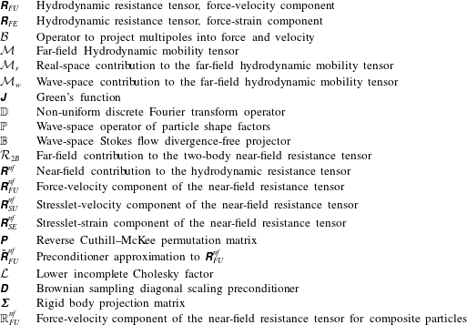
List of scalars and vectors.
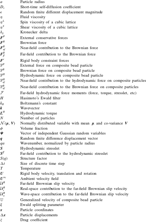
List of abbreviations.