




1 Introduction
The unsteady heat release of a flame is a source of non-isentropic temperature perturbations that are widely referred to as entropy waves (Dowling Reference Dowling1995; Dowling & Stow Reference Dowling and Stow2003; Karimi, Brear & Moase Reference Karimi, Brear and Moase2008, Reference Karimi, Brear and Moase2010). In continuous combustion systems, these temperature perturbations occur at the flame region and subsequently advect downstream. On reaching the downstream components with variable cross-sections, their acceleration or deceleration results in the generation of acoustic waves (Howe Reference Howe1975; Williams & Howe Reference Williams and Howe1975). Sound generated in this way is termed entropy noise or indirect combustion noise and is far less understood than direct combustion noise due to turbulence (Candel et al. Reference Candel, Durox, Ducruix, Birbaud, Noiray and Schuller2009; Morgans & Dúran Reference Morgans and Dúran2016). Further, indirect combustion noise constitutes an important noise source that contributes to engine core-noise and can influence thermoacoustic instabilities (Hield, Brear & Jin Reference Hield, Brear and Jin2009; Leyko, Nicoud & Poinsot Reference Leyko, Nicoud and Poinsot2009; Poinsot Reference Poinsot2017). Yet, the degree of entropy wave annihilation in gas turbine combustors is still unclear (Eckstein, Freitag & Sattelmayer Reference Eckstein, Freitag and Sattelmayer2006; Eckstein & Sattelmayer Reference Eckstein and Sattelmayer2006; Morgans, Goh & Dahan Reference Morgans, Goh and Dahan2013), indicating the need for further research on the evolution of advective entropy waves.
Many studies have focused on deriving transfer functions for the acoustic response of nozzles to entropic forcing. In their seminal work, Marble & Candel (Reference Marble and Candel1977) developed a one-dimensional, linear theory for a compact nozzle. Later studies extended the original theory to less restrictive conditions that include non-compact nozzles (Stow, Dowling & Hynes Reference Stow, Dowling and Hynes2002; Moase, Brear & Manzie Reference Moase, Brear and Manzie2007; Goh & Morgans Reference Goh and Morgans2011; Giauque, Huet & Clero Reference Giauque, Huet and Clero2012; Dúran & Moreau Reference Dúran and Moreau2013) and nonlinear dynamics (Moase et al. Reference Moase, Brear and Manzie2007; Huet & Giauque Reference Huet and Giauque2013). The models of Giauque et al. (Reference Giauque, Huet and Clero2012) and Dúran & Moreau (Reference Dúran and Moreau2013) were later rederived using section-integral quantities, thus extending them to include the effects of the radial deformation of entropy waves (Zheng et al. Reference Zheng, Huet, Giauque, Cléro and Ducruix2015; Emmanuelli et al. Reference Emmanuelli, Huet, Garrec and Ducruix2017, Reference Emmanuelli, Huet, Garrec and Ducruix2018). This formulation requires a fluid dynamics simulation to provide the two-dimensional flow field inside the nozzle. Recently, Fattahi et al. (Reference Fattahi, Hosseinalipour, Karimi, Saboohi and Ommi2019) extended the compact analysis to include the annihilating effects due to hydrodynamics, heat transfer, and flow stretch upon the nozzle response. Nevertheless, since these works were primarily concerned with the conversion of entropy waves into sound in a nozzle, the upstream evolution of entropy waves was not investigated. Also, recently, the theory of Marble & Candel (Reference Marble and Candel1977) has been extended to the case of a multi-component gas. This led to the discovery of a different component of indirect combustion noise, termed compositional noise (Magri, O’Brien & Ihme Reference Magri, O’Brien and Ihme2016; Ihme Reference Ihme2017; Magri Reference Magri2017; Rolland, Domenico & Hochgreb Reference Rolland, Domenico and Hochgreb2018).
So far, the predictions of entropy conversion models have mostly been compared with inviscid flow simulations, which inherently neglect the decay of entropy waves (Moase et al. Reference Moase, Brear and Manzie2007; Goh & Morgans Reference Goh and Morgans2011; Dúran, Moreau & Poinsot Reference Dúran, Moreau and Poinsot2012). As an exception to this, Leyko et al. (Reference Leyko, Moreau, Nicoud and Poinsot2011) compared the Marble & Candel (Reference Marble and Candel1977) model predictions with a direct numerical simulation (DNS) of the experimental set-up of Bake, Kings & Röhle (Reference Bake, Kings and Röhle2008) and Bake et al. (Reference Bake, Richter, Mühlbauer, Kings, Röhle, Thiele and Noll2009) and reported a good agreement. This was achieved in a set-up with long-wavelength entropy waves and an isothermal base flow. However, more recent numerical simulations of heat transferring flows revealed that advective entropy waves in channels could significantly deviate from being one-dimensional fronts (Fattahi, Hosseinalipour & Karimi Reference Fattahi, Hosseinalipour and Karimi2017). Studies on the conversion of entropy waves to sound in turbine stages (Cumpsty & Marble Reference Cumpsty and Marble1977; Dúran et al. Reference Dúran, Leyko, Moreau, Nicoud and Poinsot2013; Livebardon et al. Reference Livebardon, Moreau, Gicquel, Poinsot and Bouty2016) have supplied their models with realistic entropy waves. Nonetheless, this required experimental data or high-fidelity large-eddy simulations of the entire combustor. With the exception of these high-order models, all entropy noise studies have assumed that the entropy wave impinging upon the nozzle inlet is spatially uniform. However, there is now an emerging body of evidence indicating that advection of entropy waves through a combustor flow field includes sophisticated time-dependent patterns, which readily violate this assumption (Brear, Carolan & Karimi Reference Brear, Carolan and Karimi2010; Fattahi et al. Reference Fattahi, Hosseinalipour and Karimi2017). Low-order modelling of such dynamics remains as an ongoing challenge.
The early dispersion model of Sattelmayer (Reference Sattelmayer2003) is the first to account for the influence of combustion chamber aerodynamics on an advecting entropy perturbation. The modelling approach treated an experimental dual-fuel burner as a single-input single-output (SISO) dynamical system. The impulse response of the system was taken as the probability density function of the residence time and was modelled by a rectangular pulse to yield an analytic expression for the system transfer function. More recently, Goh & Morgans (Reference Goh and Morgans2013) added a dissipation factor to the dispersion model of Sattelmayer (Reference Sattelmayer2003) to account for the decay of entropy waves and incorporated it into a thermoacoustic model. Subsequently, these authors showed that entropy noise could act constructively or destructively on combustor stability depending on the levels of dissipation and dispersion.
In a separate work, Morgans et al. (Reference Morgans, Goh and Dahan2013) investigated the dissipation and shear dispersion of entropy waves. This was performed through an incompressible, direct numerical simulation of an entropy perturbation advected by a fully developed, turbulent channel flow. Dissipation of the entropy wave was defined in terms of the total thermal energy and, as would be expected for an adiabatic system, was found to be negligible. Shear dispersion was modelled using the Sattelmayer (Reference Sattelmayer2003) model, but in this case it was shown that the response is better captured by a Gaussian pulse. Finally, a simple case study using the modified dispersion model and conditions representative of a typical gas turbine combustor revealed that the magnitude of the transfer function is significant up to the frequencies relevant to combustion instabilities (several hundred hertz). This was in keeping with the numerical and experimental evidence suggesting that entropy noise could influence combustion stability (Hield & Brear Reference Hield and Brear2008; Hield et al. Reference Hield, Brear and Jin2009; Motheau, Nicoud & Poinsot Reference Motheau, Nicoud and Poinsot2014). Recently, Giusti et al. (Reference Giusti, Worth, Mastorakos and Dowling2017) modelled the magnitude of the transfer function directly (instead of the system response) with an exponential function and showed that it scales well with a local Helmholtz number based on the entropy wavelength and streamwise position. Although not realistic for a real combustor, the entropic forcing used was a single frequency sinusoid, and thus, any effects due to modal coupling were not included. Similarly, Waßmer et al. (Reference Waßmer, Schuermans, Paschereit and Moeck2016) included the effect of turbulence on the decay of entropy waves by adding an effective diffusivity, developed through the analytical solution of an advection-diffusion equation.
In keeping with the linear one-dimensional framework of nozzle response studies, the models developed for the decay of entropy waves in combustors (Sattelmayer Reference Sattelmayer2003; Morgans et al. Reference Morgans, Goh and Dahan2013; Giusti et al. Reference Giusti, Worth, Mastorakos and Dowling2017) can readily be integrated into the existing thermoacoustic models. Importantly, the assumption of linear dynamics in models of entropy waves is not entirely based on the physics of these perturbations but is simply phenomenological. This is because the physical mechanisms responsible for the attenuation of entropy waves are still largely unexplored (Fattahi et al. Reference Fattahi, Hosseinalipour and Karimi2017). Further, the opposing findings about the influence of entropy noise on combustion stability (Eckstein & Sattelmayer Reference Eckstein and Sattelmayer2006; Eckstein et al. Reference Eckstein, Freitag and Sattelmayer2006; Hield et al. Reference Hield, Brear and Jin2009) imply that flow processes downstream of the flame play an important role in the wave attenuation.
Despite these, the existing low-order models of entropy waves either totally ignore turbulence and heat transfer or represent their complex effects by a simple dissipation factor. Thus, a more generic approach that allows for development of nonlinear models is warranted. Further, the one-dimensional treatment of the entropy perturbation implies a SISO approach to the description of entropy waves (Dowling & Morgans Reference Dowling and Morgans2005; Lieuwen Reference Lieuwen2012). However, an experimental (Brear et al. Reference Brear, Carolan and Karimi2010) study and a recent numerical (Fattahi et al. Reference Fattahi, Hosseinalipour and Karimi2017) study have shown that entropy perturbations could become spatially uncorrelated. The threshold frequency at which correlation starts to breakdown, and therefore the amount of thermal energy that is filtered out by application of an average depends on the thermal boundary conditions and the hydrodynamics of the flow (Fattahi et al. Reference Fattahi, Hosseinalipour and Karimi2017). Consequently, it is imperative to model entropy waves as a multi-input multi-output (MIMO) system. This, in turn, calls for prediction of the spatio-temporal dynamics of these waves. Yet, currently there is no low-order modelling tool for this purpose. To address this issue, the current work uses a novel dynamical approach and develops a low-order model that can simulate the amplitude decay and spatial distortion of a two-dimensional entropy wave. The model is capable of predicting both spatial and temporal features of an entropy wave. This is based on reduction of the data generated by a DNS of compressible, fully developed, turbulent channel flow with adiabatic and heat transferring external walls and an added Gaussian entropy perturbation.
2 Numerical simulation
Fluid flow is governed by (2.1a )–(2.1c ) as follows:
 $$\begin{eqnarray}\displaystyle & \displaystyle \frac{\unicode[STIX]{x2202}\unicode[STIX]{x1D70C}}{\unicode[STIX]{x2202}t}+\frac{\unicode[STIX]{x2202}\unicode[STIX]{x1D70C}u_{j}}{\unicode[STIX]{x2202}x_{j}}=0, & \displaystyle\end{eqnarray}$$
 $$\begin{eqnarray}\displaystyle & \displaystyle \frac{\unicode[STIX]{x2202}\unicode[STIX]{x1D70C}u_{i}}{\unicode[STIX]{x2202}t}+\frac{\unicode[STIX]{x2202}\unicode[STIX]{x1D70C}u_{i}u_{j}}{\unicode[STIX]{x2202}x_{j}}=-\frac{\unicode[STIX]{x2202}p}{\unicode[STIX]{x2202}x_{i}}+\frac{\unicode[STIX]{x2202}\unicode[STIX]{x1D70F}_{ij}}{\unicode[STIX]{x2202}x_{j}}+\unicode[STIX]{x1D70C}g_{i}, & \displaystyle\end{eqnarray}$$
 $$\begin{eqnarray}\displaystyle & \displaystyle \unicode[STIX]{x1D70C}c_{p}\left(\frac{\unicode[STIX]{x2202}T}{\unicode[STIX]{x2202}t}+u_{i}\frac{\unicode[STIX]{x2202}T}{\unicode[STIX]{x2202}x_{i}}\right)=\frac{\unicode[STIX]{x2202}p}{\unicode[STIX]{x2202}t}+u_{i}\frac{\unicode[STIX]{x2202}p}{\unicode[STIX]{x2202}x_{i}}+k\frac{\unicode[STIX]{x2202}^{2}T}{\unicode[STIX]{x2202}x_{i}\unicode[STIX]{x2202}x_{i}}+\unicode[STIX]{x1D70F}_{ij}\frac{\unicode[STIX]{x2202}u_{i}}{\unicode[STIX]{x2202}x_{j}}, & \displaystyle\end{eqnarray}$$
 $\unicode[STIX]{x1D70C},u_{i},p$
and
 $T$
are density, velocity, pressure and temperature, respectively. Derivatives of the dependent variables are with respect to time
 $t$
and the spatial coordinates
 $x_{i}$
. The constants
 $c_{p},k$
, and
 $g_{i}$
are the specific heat at constant pressure, thermal conductivity, and the gravitational acceleration vector, respectively. A repeated subscript implies summation over the index range
 $i=1,2,3$
.
The shear stress tensor
 $\unicode[STIX]{x1D70F}_{ij}$
for a Newtonian fluid is related to the strain rate tensor
 $\unicode[STIX]{x1D61A}_{ij}$
through (2.2a
), where
 $\unicode[STIX]{x1D707}$
is the dynamic viscosity of the fluid. The strain rate tensor
 $\unicode[STIX]{x1D61A}_{ij}$
is related to the velocity gradients by (2.2b
), and (2.2c
) states the ideal gas law, where
 $R$
is the specific gas constant:
 $$\begin{eqnarray}\displaystyle & \displaystyle \unicode[STIX]{x1D70F}_{ij}-{\textstyle \frac{1}{3}}\unicode[STIX]{x1D70F}_{kk}=2\unicode[STIX]{x1D707}\left(\unicode[STIX]{x1D61A}_{ij}-{\textstyle \frac{1}{3}}\unicode[STIX]{x1D61A}_{kk}\right), & \displaystyle\end{eqnarray}$$
 $$\begin{eqnarray}\displaystyle & \displaystyle \unicode[STIX]{x1D61A}_{ij}=\frac{1}{2}\left(\frac{\unicode[STIX]{x2202}u_{i}}{\unicode[STIX]{x2202}x_{j}}+\frac{\unicode[STIX]{x2202}u_{j}}{\unicode[STIX]{x2202}x_{i}}\right), & \displaystyle\end{eqnarray}$$
 $$\begin{eqnarray}\displaystyle & \displaystyle p=\unicode[STIX]{x1D70C}RT. & \displaystyle\end{eqnarray}$$
2.1 Flow solver
The governing system of (2.1) and (2.2) is solved using a variant of the Imperial College in-house DNS flow solver with the acronym BOFFIN (boundary fitted flow integrator) (Jones & Wille Reference Jones and Wille1996; Mare & Jones Reference Mare and Jones2003; Paul & Molla Reference Paul and Molla2012; Alzwayi, Paul & Navarro-Martinez Reference Alzwayi, Paul and Navarro-Martinez2014). The flow solver is a low Mach number formulation and therefore neglects the terms
 $\unicode[STIX]{x2202}p/\unicode[STIX]{x2202}t+u_{i}(\unicode[STIX]{x2202}p/\unicode[STIX]{x2202}x_{i})$
and
 $\unicode[STIX]{x1D70F}_{ij}(\unicode[STIX]{x2202}u_{i}/\unicode[STIX]{x2202}x_{j})$
in (2.1c
). The neglected terms are namely the total derivative of pressure and frictional heating, respectively, and are negligible at low Mach number (Mare Reference Mare2002). Nonetheless, flows in gas turbine combustors are at low Mach number (the bulk flow Mach number of 0.1–0.2 (Lefebvre & Ballal Reference Lefebvre and Ballal2010)), thus justifying the use of the particular DNS solver.
The spatial and temporal derivatives in the governing equations are discretised using second-order accurate schemes on a staggered grid arrangement with the exception of the nonlinear term
 $\unicode[STIX]{x2202}\unicode[STIX]{x1D70C}u_{i}u_{j}/\unicode[STIX]{x2202}x_{j}$
in (2.1b
) for which an energy conserving scheme is used (Morinishi Reference Morinishi1995). The time-marching scheme is implicit. Pressure and velocity fields are obtained using a type of ‘semi-implicit method for pressure linked equations’ (known as SIMPLE) algorithm (Paul & Molla Reference Paul and Molla2012). The Poisson-like pressure correction equation is discretised using the pressure smoothing approach of Rhie & Chow (Reference Rhie and Chow1983), which prevents decoupling of pressure and velocity fields at even and odd grid nodes. The BI-CGSTAB (Vorst Reference Vorst1992) and ICCG (Kershaw Reference Kershaw1978) matrix solvers are used for velocity and pressure, respectively.
In real gas turbine combustors, cooling air flows externally around the walls. Hence, the current study adds a convective thermal boundary condition to the external surface of the duct according to which the temperature at the walls satisfies the heat flux equality in (2.3), where
 $(\unicode[STIX]{x2202}T/\unicode[STIX]{x2202}y)|_{wall}$
is the temperature gradient at the wall,
 $T_{wall}$
is the wall temperature and
 $h$
is the convective heat transfer coefficient between the wall and a hypothetical external flow (not simulated) at surrounding temperature
 $T_{\infty }=300~\text{K}$
as follows:
 $$\begin{eqnarray}k\left.\frac{\unicode[STIX]{x2202}T}{\unicode[STIX]{x2202}y}\right|_{wall}=h[T_{wall}(x)-T_{\infty }].\end{eqnarray}$$
The left-hand side of (2.3) is the heat flux from the stationary (no-slip) fluid layer to the wall according to Fick’s law and the right-hand side is the heat flux from the wall to the hypothetical external flow according to Newton’s law of cooling. The wall is assumed infinitesimally thick and thus conduction of heat through the wall itself is not considered. This thermal boundary condition enables specification of adiabatic walls through setting
 $h=0~\text{Wm}^{-2}~\text{K}^{-1}$
and streamwise varying heat transfer through setting a finite value. Experimental and numerical studies have shown that the heat transfer coefficient on the liner of gas turbine combustors is in the range
 $h=200{-}800~\text{Wm}^{-2}~\text{K}^{-1}$
(Bailey et al.
Reference Bailey, Intile, Fric, Tolpadi, Nirmalan and Bunker2003). As part of the current study, simulations were performed for the cases of
 $h=200~\text{Wm}^{-2}~\text{K}^{-1}$
and
 $h=800~\text{Wm}^{-2}~\text{K}^{-1}$
. The results from these cases show that the width of the wave in the wall-normal direction is smaller at the larger heat transfer coefficient. Nonetheless, the difference is not significant and thus, only results from the case of
 $h=200~\text{Wm}^{-2}~\text{K}^{-1}$
are presented in the work that follows.
2.2 Direct numerical simulation of turbulent channel flow
The simulated flow is a compressible, fully developed, turbulent airflow in a channel at friction Reynolds number
 $Re_{\unicode[STIX]{x1D70F}}=u_{\unicode[STIX]{x1D70F}}\unicode[STIX]{x1D6FF}/\unicode[STIX]{x1D708}=180$
, where
 $u_{\unicode[STIX]{x1D70F}}$
is the friction velocity,
 $\unicode[STIX]{x1D6FF}$
is the channel half-height and
 $\unicode[STIX]{x1D708}$
is the kinematic viscosity. This corresponds to a Mach number
 $M_{c}=0.15$
based on the mean centre line velocity. An instructive schematic of the channel configuration is shown in figure 1. The size of the simulation domain is
 $4\unicode[STIX]{x03C0}\unicode[STIX]{x1D6FF}\times 2\unicode[STIX]{x1D6FF}\times \unicode[STIX]{x03C0}\unicode[STIX]{x1D6FF}$
in the streamwise (
 $x$
), wall-normal (
 $y$
) and spanwise (
 $z$
) directions, respectively. In each direction, the domain is discretised with
 $368\times 128\times 128$
nodes. Periodic boundary conditions are imposed in the streamwise and spanwise directions and the no-slip boundary condition at the walls. In the periodic directions the grid is uniform with
 $\unicode[STIX]{x0394}x^{+}=u_{\unicode[STIX]{x1D70F}}\unicode[STIX]{x0394}x/\unicode[STIX]{x1D708}=6.1$
and
 $\unicode[STIX]{x0394}z^{+}=u_{\unicode[STIX]{x1D70F}}\unicode[STIX]{x0394}z/\unicode[STIX]{x1D708}=4.4$
. In the wall-normal direction the grid is stretched from
 $\unicode[STIX]{x0394}y_{w}^{+}=u_{\unicode[STIX]{x1D70F}}\unicode[STIX]{x0394}y_{w}/\unicode[STIX]{x1D708}=0.15$
at the wall to
 $\unicode[STIX]{x0394}y_{c}^{+}=u_{\unicode[STIX]{x1D70F}}\unicode[STIX]{x0394}y_{c}/\unicode[STIX]{x1D708}=5$
at the centre line according to
 $\unicode[STIX]{x0394}y_{j+1}/\unicode[STIX]{x0394}y_{j}=SF$
, where
 $j=1,2,\ldots ,63$
is the cell number (
 $j=1$
is the cell at the wall and
 $j=63$
is the cell at the centre line) and
 $SF=1.05$
is the stretch factor. The pressure of the base flow is
 $\overline{p}=1\times 10^{5}~\text{Pa}$
and the corresponding temperature is
 $\overline{T}=1500~\text{K}$
.
Channel configuration.

The cross-sectional profiles of the mean velocity and mean square of the turbulent fluctuations are shown in figure 2. Mean and fluctuating velocity components are indicated by an overbar (
 $\bar{\text{ }}$
) and a prime (
 $^{\prime }$
), respectively. Velocity is non-dimensionalised by the wall-shear velocity
 $u_{\unicode[STIX]{x1D70F}}=\sqrt{\unicode[STIX]{x1D70F}_{w}/\unicode[STIX]{x1D70C}}$
, where
 $\unicode[STIX]{x1D70F}_{w}$
is the flow shear stress on the wall. The wall-normal coordinate
 $y^{+}=(u_{\unicode[STIX]{x1D70F}}y)/\unicode[STIX]{x1D708}$
, with
 $\unicode[STIX]{x1D708}$
being the kinematic viscosity, is the distance from the wall in wall-units. The profiles collapse with the canonical data of Kim, Moin & Moser (Reference Kim, Moin and Moser1987), thus confirming that the grid is sufficiently fine and that the flow condition has been reached. The spatial variability of the flow velocity is elucidated by a snapshot of the instantaneous velocity field (velocity is non-dimensionalised by the local speed of sound) shown in figure 3 for a streamwise cross-section at midspan.
The flow (a) mean velocity and (b) mean square of turbulent fluctuations collapse with the canonical data of Kim et al. (Reference Kim, Moin and Moser1987): —— present study, ▫ Kim et al. (Reference Kim, Moin and Moser1987).

Instantaneous velocity components in the (a) streamwise, (b) wall-normal and (c) spanwise directions non-dimensionalised by the speed of sound.

2.3 Entropy wave
Entropy is related to temperature and pressure through the thermodynamic equation (2.4), where
 $s$
is entropy as follows:
 $$\begin{eqnarray}\frac{\text{d}s}{c_{p}}=\frac{\text{d}T}{T}-\frac{R}{c_{p}}\frac{\text{d}p}{p}.\end{eqnarray}$$
Conversion of entropy waves to acoustic waves is subject to mean flow acceleration (Williams & Howe Reference Williams and Howe1975), which is absent in the current configuration. Also, the aerodynamic sources of noise are insignificant in the considered channel flow (Crighton Reference Crighton1975). Hence, in keeping with the previous studies of entropy wave decay (Morgans et al.
Reference Morgans, Goh and Dahan2013; Fattahi et al.
Reference Fattahi, Hosseinalipour and Karimi2017; Giusti et al.
Reference Giusti, Worth, Mastorakos and Dowling2017), the pressure term
 $\text{d}p/p$
in (2.4) is ignored and entropy fluctuations scale with temperature fluctuations. The entropy wave is therefore added to the flow by perturbing the temperature of the base flow in a cross-section immediately downstream of the channel inlet. The method resembles that of the entropy wave generator (known as EWG) used in experimental studies (Bake et al.
Reference Bake, Kings and Röhle2008, Reference Bake, Richter, Mühlbauer, Kings, Röhle, Thiele and Noll2009) of entropy noise, which adds entropy waves to an accelerating tube flow by means of a heating module. In the current problem the temperature fluctuations induced by turbulence are smaller than the temperature fluctuation imposed on the flow by several orders of magnitude.
The temporal profile chosen for the temperature perturbation is Gaussian and is given by (2.5) as follows:
 $$\begin{eqnarray}\frac{\unicode[STIX]{x0394}T}{\overline{T}}=A\exp \left[-\frac{(\unicode[STIX]{x1D70F}-\unicode[STIX]{x1D707})^{2}}{2\unicode[STIX]{x1D70E}^{2}}\right],\end{eqnarray}$$
where
 $\unicode[STIX]{x0394}T/\overline{T}=(T-\overline{T})/\overline{T}$
is the instantaneous amplitude of the perturbation relative to the base flow temperature
 $\overline{T}$
,
 $A$
is the peak amplitude of the perturbation,
 $\unicode[STIX]{x1D70F}$
is non-dimensional time,
 $\unicode[STIX]{x1D707}$
is the non-dimensional time at which the perturbation reaches its peak amplitude and
 $\unicode[STIX]{x1D70E}$
is the standard deviation of the perturbation that controls the duration of the temperature forcing. Here,
 $\unicode[STIX]{x1D70F}=(\overline{U}_{bulk}/L)t$
, where,
 $\overline{U}_{bulk}$
is the bulk flow velocity,
 $L$
is the channel length and therefore
 $\unicode[STIX]{x1D70F}$
is multiples of the mean residence time. At every time step the instantaneous amplitude of the perturbation is uniform over the plane cross-section at which it is added. The present study uses
 $A=0.1$
,
 $\unicode[STIX]{x1D70E}=0.1$
and
 $\unicode[STIX]{x1D707}=0.5$
. The process of generating the entropy wave is illustrated in figure 4. The graph in figure 4(a) shows the Gaussian perturbation used in the present study to perturb the temperature in the plane cross-section shown in figure 4(b).
Entropy wave generated by perturbing the temperature in a cross-section immediately downstream of the channel inlet. The temporal profile of the perturbation is Gaussian as per equation (2.5) with
 $A=0.1$
,
 $\unicode[STIX]{x1D70E}=0.1$
and
 $\unicode[STIX]{x1D707}=0.5$
.

2.4 Entropy wave advection
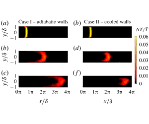
Snapshots of the advecting entropy wave after it has been added to the flow are shown in the left and right columns of figure 5 for the cases of adiabatic and convective heat loss at the walls, respectively. In each case the snapshot in (a,d) shows the state of the entropy wave as soon as it has been added to the flow i.e. when the forcing of temperature at the insert plane has ceased (in figure 4 this corresponds to
 $\unicode[STIX]{x1D70F}\approx 0.07$
). The snapshots in (b,e,c,f) show the states of the entropy wave when it reaches the channel half-length and outlet, respectively. The time difference between the snapshots is the same.
The maximum amplitude shortly after the generation of the entropy wave (in figure 5
a,d) is
 $\unicode[STIX]{x0394}T/\overline{T}=0.06$
, which is lower than the peak value
 $A=0.1$
of the added Gaussian perturbation. The
 $40\,\%$
reduction in amplitude occurs in the time taken to generate the entropy wave, that is, in a non-dimensional time interval
 $\unicode[STIX]{x0394}\unicode[STIX]{x1D70F}=0.07$
(see figure 4
a). By the time the wave reaches the channel half-length (figure 5
b,e) and outlet (figure 5
c,f), the maximum amplitude is
 $\unicode[STIX]{x0394}T/\overline{T}\approx 0.025$
and
 $\unicode[STIX]{x0394}T/\overline{T}\approx 0.015$
, respectively. Thus, a
 $40\,\%$
reduction in amplitude within
 $\unicode[STIX]{x0394}\unicode[STIX]{x1D70F}=0.25$
during the generation of the wave is followed by further
 $35\,\%$
and
 $10\,\%$
reductions within the successive
 $\unicode[STIX]{x0394}\unicode[STIX]{x1D70F}=0.5$
intervals. It is clear that a profound decay occurs while the entropy wave is being generated. The reason for this sharp drop in wave strength at the generation stage is twofold. First, the strong temperature gradient developed near the insert plane presents a major driving force for heat transfer by molecular diffusion. In addition, turbulent mixing is also more effective than that at later stages because the thermal energy of the added entropy wave is distributed over a broadband frequency range (the width of the frequency spectrum depends on the value used for
 $\unicode[STIX]{x1D70E}$
in (2.5) – the smaller
 $\unicode[STIX]{x1D70E}$
is the wider the frequency spectrum). The thermal energy contained in the high-frequency components of the perturbation that have small wavelengths of order comparable or smaller than those of the turbulence undergo strong turbulent diffusion (Fattahi et al.
Reference Fattahi, Hosseinalipour and Karimi2017). The extent of amplitude decay during the generation of entropy waves is dependent on the temporal ‘sharpness’ of the added perturbation, which in the case of the artificially generated wave in the current study is controlled by the value of
 $\unicode[STIX]{x1D70E}$
in (2.5).
Convection of temperature perturbation through a fully developed, turbulent, channel flow with adiabatic walls (a–c) and convective cooling at the walls (d–f) obtained by direct numerical simulation.

In both cases (figure 5 a–f), as the entropy wave advects from the insert plane towards the channel outlet, it undergoes changes in shape, thickness and amplitude. The later discussion suggests that the amplitude decay is, in part, a consequence of the shape of the wave. Heat loss at the walls causes a reduction in amplitude directly by removing heat from the hot fluid but also indirectly through its influence upon the shape and thickness of the wave.
The uniform shape of the wave imposed at the insert plane is lost due to the spatial non-uniformity of the velocity field. The slower mean velocity near the walls causes spreading of the wave in the near wall regions. Hot and cold regions of the flow inter-penetrate each other creating temperature gradients in the wall-normal direction that enhances the molecular diffusion of heat and thus, the amplitude decay. The destructive effect of the non-uniform velocity field, which is particularly noticeable near the walls where large velocity gradients exist, is known as the shear-dispersion mechanism (Morgans et al. Reference Morgans, Goh and Dahan2013). Heat losses at the walls (figure 5 d–f) produce steeper temperature gradients in the wall-normal direction. Hence, amplitude decay especially in the near wall regions is much more profound when the walls are cooled. In fact, in this scenario the amplitude of the wave quickly drops to zero near the walls and the entropy wave vanishes close to the walls.
The spreading or thickening of the wave as it advects downstream is due to molecular and turbulent diffusion of heat from the hot fluid to the surrounding base flow. As heat is distributed over an increasingly larger volume, the amplitude of the wave decays. Further, as the wave spreads out the spectral distribution of the entropy wave becomes limited to the low frequency regions. It has already been shown that low frequency components of the entropy wave can survive turbulent flow much better than those of high frequencies (Fattahi et al. Reference Fattahi, Hosseinalipour and Karimi2017). Thus, the contribution of turbulent mixing to the overall diffusion process is progressively hindered as the wave thickens and molecular diffusion becomes the dominant diffusion mechanism. Since molecular diffusion of heat is naturally much slower than turbulent diffusion, the rate of decay of the wave amplitude slows down.
In the current study, similar to Fattahi et al. (Reference Fattahi, Hosseinalipour and Karimi2017), the term dissipation is used to refer to the decay of the wave amplitude. It is necessary to make this clarification because the definition of dissipation in the context of entropy wave attenuation is not consistent in the literature. Morgans et al. (Reference Morgans, Goh and Dahan2013) defined dissipation in terms of total thermal energy, which, in an adiabatic system, is conserved. Dissipation defined as such does not include the decay of amplitude due to the diffusion of heat from the hot fluid to the surrounding base flow. Thus, dissipation in terms of amplitude decay is a more generic definition as it includes the decay by thermal energy loss due to the sinks in the flow, but also includes the decay resulting from spreading of the wave.
3 Low-order model
The results of the direct simulation show that as the entropy wave advects through the turbulent channel flow it does not retain the initial uniform shape and amplitude. However, the established low-order modelling approach has kept with the one-dimensional outlook of studies of acoustic waves (Sattelmayer Reference Sattelmayer2003; Morgans et al. Reference Morgans, Goh and Dahan2013; Giusti et al. Reference Giusti, Worth, Mastorakos and Dowling2017). That is, the entropy wave has been integrated over the cross-section at every time step to produce a one-dimensional entropy wave with a single position and a single amplitude that are time dependent. In their approach, it is assumed that the position of the entropy wave changes at a rate equal to the bulk velocity of the isothermal flow and the modelling process concentrates exclusively on the temporal decay of the volumetric amplitude.
The current work aims to improve the aforementioned modelling approach in two respects. Firstly, it avoids making any assumption regarding the wave speed and includes the wave position as an output of the modelling process. Secondly, the entropy wave is not reduced to a one-dimensional wave through integration but instead is sectioned into streamwise cross-sections to allow the position and amplitude in each cross-section to be modelled. Hence, in the present study the terms position and amplitude refer to the positions and amplitudes from all the streamwise cross-sections, collectively.
The thermal energy at any moment in time is mainly concentrated around the position of the maximum amplitudes as shown in figure 6. The snapshot in figure 6(a) from the direct numerical simulation of the adiabatic walls case shows the state of the entropy wave once it has reached the channel half-length. The curve
 $C_{max}$
that is seen in the snapshot traces the positions of the maximum amplitudes in the streamwise cross-sections. The integrated amplitude along the curve
 $C_{max}$
is plotted as a point on the graph in figure 6(b). Shifting the curve
 $C_{max}$
upstream and downstream from its original position (where it coincides with the positions of maximum amplitudes) and plotting the integral of the amplitudes along the curve at the new positions gives the bell-like curve shown in figure 6(b). The horizontal axis of the graph in figure 6(b) is the displacement of the curve relative to its original position. The bell-like distribution shows how the thermal energy is distributed around the positions of the maximum amplitudes (i.e. around the original position of
 $C_{max}$
). Approximately 70 % of the thermal energy is concentrated around the positions of the maximum amplitude over a distance that is only 20 % of the wave thickness (the thickness of the wave being defined in this case as the distance between the curves that have an integrated amplitude that is 10 % of the peak amplitude
 $A=0.1$
). Hence, without much loss of generality the entropy wave can be represented by the curve connecting the positions of the maximum amplitudes in the streamwise cross-sections.
The snapshot of the entropy wave when it is at the channel half-length and the curve
 $C_{max}$
connecting the positions of the maximum amplitudes in the streamwise cross-sections. The amplitude is integrated along the curve as it is shifted upstream and downstream from its original position. The graph shows the integrated amplitude with respect to the displacement. A large proportion of the total thermal energy is concentrated around the positions of the maximum amplitudes.

Time series of the position and magnitude of the maximum amplitude in each streamwise cross-section of the flow are generated from the direct simulation. At every time step of the DNS, the amplitudes at all nodes in the streamwise direction with the same wall-normal coordinate
 $y$
are compared and the maximum amplitude in the streamwise section is found. The position at which the maximum temperature occurs is
 $x_{max}$
and its magnitude is
 $(\unicode[STIX]{x0394}T/\overline{T})_{max}$
. Both these quantities are a function of the wall-normal coordinate
 $y$
and the instant of time at which they are evaluated. The present study used
 $128$
nodes in the
 $y$
- or wall-normal direction and, therefore, generated
 $128$
time series of
 $x_{max}$
and
 $128$
time series of
 $(\unicode[STIX]{x0394}T/\overline{T})_{max}$
.
In the methodology that follows, the subscript
 $\{\text{ }\}_{max}$
is dropped from
 $x_{max}$
and
 $(\unicode[STIX]{x0394}T/\overline{T})_{max}=\hat{T}_{max}$
, where the caret
 $\{\hat{\text{ }}\}$
is used to indicate a non-dimensional quantity. Results are presented using the non-dimensional quantities in (3.1), where
 $\unicode[STIX]{x1D70F}$
is non-dimensional time (see (2.5)) and
 $\unicode[STIX]{x1D6FF}$
is the channel half-height as follows:
 $$\begin{eqnarray}\hat{t}=\unicode[STIX]{x1D70F},\quad \hat{x}=\frac{x_{max}}{\unicode[STIX]{x1D6FF}},\quad {\hat{y}}=\frac{y}{\unicode[STIX]{x1D6FF}}.\end{eqnarray}$$
3.1 Formulation using DNS data from the case of adiabatic walls
The model is based on the assumption that the spatio-temporal evolution of the position and amplitude of the wave in a streamwise cross-section can be described by the generic nonlinear system in (3.2), where the dot
 $\{\dot{\text{ }}\}$
indicates the derivative with respect to time and
 $T$
is the amplitude at streamwise position
 $x$
as follows:
 $$\begin{eqnarray}\displaystyle & \displaystyle {\dot{x}}=g(T,x), & \displaystyle\end{eqnarray}$$
 $$\begin{eqnarray}\displaystyle & \displaystyle {\dot{T}}=f(T,x). & \displaystyle\end{eqnarray}$$
Using the multivariate Taylor series expansion, equation (3.2) is expressed as the infinite summation in (3.3), where
 $\unicode[STIX]{x1D6F7}_{j}$
is the state vector,
 $\unicode[STIX]{x1D611}_{ij}$
is the Jacobian matrix and a repeated subscript implies summation over the range
 $i,j=1,2$
:
 $$\begin{eqnarray}\displaystyle & \displaystyle \dot{\unicode[STIX]{x1D6F7}}_{j}=\unicode[STIX]{x1D611}_{ij}\cdot \unicode[STIX]{x1D6F7}_{j}+\text{high-order terms}, & \displaystyle\end{eqnarray}$$
 $$\begin{eqnarray}\displaystyle & \displaystyle \unicode[STIX]{x1D6F7}_{j}=\left[\begin{array}{@{}c@{}}T\\ x\end{array}\right], & \displaystyle\end{eqnarray}$$
 $$\begin{eqnarray}\displaystyle & \displaystyle \unicode[STIX]{x1D611}_{ij}=\left[\begin{array}{@{}cc@{}}\displaystyle \frac{\unicode[STIX]{x2202}{\dot{T}}}{\unicode[STIX]{x2202}T} & \displaystyle \frac{\unicode[STIX]{x2202}{\dot{T}}}{\unicode[STIX]{x2202}x}\\ \displaystyle \frac{\unicode[STIX]{x2202}{\dot{x}}}{\unicode[STIX]{x2202}T} & \displaystyle \frac{\unicode[STIX]{x2202}{\dot{x}}}{\unicode[STIX]{x2202}x}\end{array}\right]. & \displaystyle\end{eqnarray}$$
The high-order terms in (3.3) are neglected and the Jacobian derivatives
 $\unicode[STIX]{x1D611}_{ij}$
are estimated from the discrete DNS data using the forward differencing scheme given by (3.4a
)–(3.4c
) as follows:
 $$\begin{eqnarray}\displaystyle & \displaystyle \frac{\unicode[STIX]{x2202}\unicode[STIX]{x1D6F7}_{j}}{\unicode[STIX]{x2202}t}\approx \frac{\unicode[STIX]{x0394}\unicode[STIX]{x1D6F7}_{j}}{\unicode[STIX]{x0394}t}=\frac{\unicode[STIX]{x1D6F7}_{j}^{t+\unicode[STIX]{x0394}t}-\unicode[STIX]{x1D6F7}_{j}^{t}}{\unicode[STIX]{x0394}t}, & \displaystyle\end{eqnarray}$$
 $$\begin{eqnarray}\displaystyle & \displaystyle \frac{\unicode[STIX]{x2202}\dot{\unicode[STIX]{x1D6F7}}_{j}}{\unicode[STIX]{x2202}T}\approx \frac{\unicode[STIX]{x0394}\dot{\unicode[STIX]{x1D6F7}}_{j}}{\unicode[STIX]{x0394}T}=\frac{\dot{\unicode[STIX]{x1D6F7}}_{j}^{t+\unicode[STIX]{x0394}t}-\dot{\unicode[STIX]{x1D6F7}}_{j}^{t}}{T^{t+\unicode[STIX]{x0394}t}-T^{t}}, & \displaystyle\end{eqnarray}$$
 $$\begin{eqnarray}\displaystyle & \displaystyle \frac{\unicode[STIX]{x2202}\dot{\unicode[STIX]{x1D6F7}}_{j}}{\unicode[STIX]{x2202}x}\approx \frac{\unicode[STIX]{x0394}\dot{\unicode[STIX]{x1D6F7}}_{j}}{\unicode[STIX]{x0394}x}=\frac{\dot{\unicode[STIX]{x1D6F7}}_{j}^{t+\unicode[STIX]{x0394}t}-\dot{\unicode[STIX]{x1D6F7}}_{j}^{t}}{x^{t+\unicode[STIX]{x0394}t}-x^{t}}, & \displaystyle\end{eqnarray}$$
 $\unicode[STIX]{x0394}t$
is the simulation time step,
 $\unicode[STIX]{x1D6F7}_{i}^{t}$
are the states at time
 $t$
, and,
 $T^{t}$
and
 $x^{t}$
are the amplitude and position of the wave, respectively, in a streamwise cross-section at time
 $t$
.
The Pearson correlation
 $\text{corr}(\unicode[STIX]{x1D611}_{ij},\unicode[STIX]{x1D6F7}_{i})$
between the estimated Jacobian derivatives
 $\unicode[STIX]{x1D611}_{ij}$
and the states
 $\unicode[STIX]{x1D6F7}_{j}$
is tabulated in table 1 (LeBlanc Reference LeBlanc2004). It is noted that the Jacobian derivative
 $J_{12}$
(gradient of the decay rate) is strongly correlated with both amplitude and position. Correlation with both states opposed to correlation with a single state is expected because amplitude and position are not independent. That is, in the absence of heat sources the amplitude decays as the wave advects downstream and the two states must be inversely proportional. Hence,
 $J_{12}$
correlates positively with
 $T$
but negatively with
 $x$
. The fact that the Jacobian derivative
 $J_{12}$
is not constant is an indication that the dynamics of amplitude decay are nonlinear. The Jacobian derivatives
 $J_{11},J_{21}$
and
 $J_{22}$
are poorly correlated with the states. This suggests that they can be assumed constant, which includes the possibility of them being zero. It is important to highlight that if
 $J_{21}$
and
 $J_{22}$
are non-zero, then the wave speed is a function of amplitude
 $T$
and position
 $x$
, as these terms couple the wave speed
 ${\dot{x}}$
to the states. If
 $J_{21}$
and
 $J_{22}$
are zero the wave speed is constant.
Pearson correlation coefficient of Jacobian derivatives (
 $\unicode[STIX]{x1D611}_{ij}$
) and states (
 $x,T$
).

The position and amplitude in the streamwise cross-section at
 ${\hat{y}}=0.17$
are shown with respect to time in figures 7(a) and 7(b). The trends of position and amplitude in the streamwise cross-sections at other wall-normal positions are the same and the discussion that follows about the trends at
 ${\hat{y}}=0.17$
applies for any wall-normal position. The linear relation between position and time in figure 7(a) confirms that the wave speed is constant. The non-zero position at
 $\hat{t}=0$
is the streamwise location of the insert plane at which the entropy wave is added to the flow. The slope of the line in figure 7(a) is the non-dimensional wave speed in the streamwise cross-section at
 ${\hat{y}}=0.17$
with the value of
 $\dot{\hat{x}}\approx 15.5$
. This corresponds to a velocity non-dimensionalised with respect to the friction velocity
 ${\dot{x}}^{+}\approx 19.5$
. From the mean velocity profile of the isothermal flow shown in figure 2, the mean velocity at the streamwise cross-section
 ${\hat{y}}=0.17$
(
 $y^{+}\approx 150$
in wall units) is
 $\overline{u}_{1}^{+}=18.3$
. Hence, the wave speed
 $\dot{\hat{x}}$
in the streamwise cross-section at
 ${\hat{y}}=0.17$
is within
 $7\,\%$
of the mean velocity of the isothermal flow. This confirms the validity of the assumption made in the previous studies (Sattelmayer Reference Sattelmayer2003; Morgans et al.
Reference Morgans, Goh and Dahan2013) that the entropy wave advects at the same velocity as the isothermal flow and thus, may be treated as a passive scalar. The data points in figure 7(a) show a linear trend. However, for perturbations with peak amplitudes much larger than
 $A=0.1$
, the validity of the passive scalar assumption is dubious as evidence exists that the entropy wave does influence the flow hydrodynamics (Hosseinalipour et al.
Reference Hosseinalipour, Fattahi, Afshari and Karimi2017). The function obtained by fitting the data with a least mean squares approach is given by (3.5), where
 $\unicode[STIX]{x1D703}_{1}$
is the fitting function to be determined. Equation (3.5) provides the form of the general equation (3.2a
):
 $$\begin{eqnarray}\dot{\hat{x}}=\unicode[STIX]{x1D703}_{1}({\hat{y}}).\end{eqnarray}$$
Plots of (a) the position of the maximum temperature perturbation with respect to time and (b) the decay rate with respect to the amplitude in a streamwise cross-section near the centre line for the case of adiabatic walls: ▫ DNS, — ⋅ — linear fit, —— quadratic fit.

Table 1 suggests that the dynamics of amplitude decay are nonlinear due to observation of a non-zero correlation between the Jacobian derivative
 $J_{12}$
and the states (the Jacobian of a linear system is invariant). This is confirmed by plotting the time derivative of amplitude (decay rate) with respect to the amplitude, which is shown in figure 7(b) for the streamwise cross-section at
 ${\hat{y}}=0.17$
. Further, since the decay rate is the time derivative of amplitude, it is convenient to plot it with respect to amplitude. At zero amplitude the wave has completely dissipated and, consequently, the decay rate is set to zero. The data point at the origin is added manually to the time series taken from the DNS because the simulation is terminated once the amplitude becomes of the same order as the turbulent fluctuations, at which point the wave practically has vanished. The phenomenological modelling approach taken by the previous studies effectively assumes that the relation between the decay rate and amplitude in figure 7(b) is linear. The linear fit is a particular form of (3.2b
), which, when integrated gives an exponentially decaying amplitude precisely as it is being viewed by the previous studies (Giusti et al.
Reference Giusti, Worth, Mastorakos and Dowling2017). However, the plot in figure 7(b) shows that for amplitudes
 $\hat{T}>0.02$
the linear approximation underestimates the decay rate during the initial stages of the wave advection and overestimates it during the final stages. The linear approximation is only capable of capturing the dynamics of the decay for amplitudes less than
 $2\,\%$
of the base flow temperature. In contrast to previous studies, the current study captures the trend of the data points in figure 7(b) by a least squares quadratic fit as per equation (3.6) – instead of a linear one:
 $$\begin{eqnarray}\dot{\hat{T}}=\unicode[STIX]{x1D703}_{2}({\hat{y}})\hat{T}^{2}.\end{eqnarray}$$
The slope of the quadratic fit in figure 7(b), which is the rate of amplitude decay, decreases with the amplitude. This is in keeping with the discussion of the DNS results in § 2. That is turbulent and molecular transport are strong during the initial stages of the wave advection thus causing a fast decay at these stages. Later, the slower molecular diffusion mechanism is dominant and results in a slower decay.
The above methodology produces a particular version of the general system of (3.2a )–(3.2b ) given by (3.5) and (3.6). Nonetheless, the time series were obtained from the DNS of the channel with adiabatic walls. Applying the same methodology to the time series obtained from the DNS of the channel with convective heat loss at the walls reveals that (3.5) and (3.6) can also be used in the non-adiabatic case but minor adjustments are necessary.
The decay rate and amplitude relation in the (a) near wall, (b) in between near wall and core flow and (c) core flow regions in the case of convective heat loss at the walls: ▫ DNS, —— fit.

3.2 Adjustment for the case of heat loss at the walls
The position of the wave in the case of heat loss at the walls is well described by (3.5) in every streamwise cross-section. However, unlike the case of adiabatic walls, the amplitude decay cannot be approximated properly by (3.6) in every streamwise cross-section. When convective heat loss is taking place at the channel walls, the exponent of the term on the right-hand side of (3.6) depends on the distance of the streamwise cross-section from the wall. The value of the exponent, which is hereafter designated as
 $\unicode[STIX]{x1D6FD}({\hat{y}})$
, comes from the fit type that is used to approximate the relation between the
 $(\hat{T},\dot{\hat{T}})$
data points in a streamwise cross-section at wall-normal coordinate
 ${\hat{y}}$
. It transitions from
 $\unicode[STIX]{x1D6FD}=2$
in the core flow to
 $\unicode[STIX]{x1D6FD}=1$
and then to
 $\unicode[STIX]{x1D6FD}=0.5$
in the near wall regions, as shown in figure 8 for three randomly chosen streamwise cross-sections between the wall and the centre line. The current work considers a piecewise and a continuous variation of the
 $\unicode[STIX]{x1D6FD}({\hat{y}})$
between the channel walls.
The piecewise
 $\unicode[STIX]{x1D6FD}({\hat{y}})$
is obtained through the use of the Akaike information criterion (AIC) (Akaike Reference Akaike2011). The fit types shown in figure 8 are all made to the data points in the streamwise cross-sections. According to the AIC, the fit type with the largest relative likelihood of being the best fit is the appropriate choice for any particular streamwise cross-section. The Akaike weight criterion is further discussed in the context of the current work in appendix A.
The continuous
 $\unicode[STIX]{x1D6FD}({\hat{y}})$
that is used in the current work is given by (3.7), which gives
 $\unicode[STIX]{x1D6FD}=2$
at the channel centre line (
 ${\hat{y}}=0$
) and
 $\unicode[STIX]{x1D6FD}=0.5$
at the channel walls (
 ${\hat{y}}=\pm 1$
) in keeping with the observations made in figure 8:
 $$\begin{eqnarray}\unicode[STIX]{x1D6FD}({\hat{y}})=2-1.5{\hat{y}}^{2}.\end{eqnarray}$$
Higher powers were tested and resulted in poor performance of the low-order model away from the channel centre line, where the values of
 $\unicode[STIX]{x1D6FD}$
were too high.
3.3 Generic low-order model
The low-order model formulated for the case of the channel with adiabatic walls given by (3.5) and (3.6) can be generalised to (3.8), where
 $\unicode[STIX]{x1D6FD}({\hat{y}})$
depends on the thermal boundary condition at the walls:
 $$\begin{eqnarray}\displaystyle & \displaystyle \dot{\hat{x}}=\unicode[STIX]{x1D703}_{1}({\hat{y}}), & \displaystyle\end{eqnarray}$$
 $$\begin{eqnarray}\displaystyle & \displaystyle \dot{\hat{T}}+\unicode[STIX]{x1D703}_{2}({\hat{y}})\hat{T}^{\unicode[STIX]{x1D6FD}({\hat{y}})}=0. & \displaystyle\end{eqnarray}$$
For adiabatic walls, it is
 $\unicode[STIX]{x1D6FD}({\hat{y}})=2$
for
 $-1\leqslant {\hat{y}}\leqslant 1$
. In the case of convective heat loss at the walls,
 $\unicode[STIX]{x1D6FD}({\hat{y}})$
varies from
 $\unicode[STIX]{x1D6FD}(0)=2$
at the centre line to
 $\unicode[STIX]{x1D6FD}(\pm 1)=0.5$
at the channel walls. The current work considers a piecewise and a continuous variation of
 $\unicode[STIX]{x1D6FD}({\hat{y}})$
over the channel cross-section in the case of convective heat loss at the walls. In the case of piecewise
 $\unicode[STIX]{x1D6FD}({\hat{y}})$
, the
 $\unicode[STIX]{x1D6FD}({\hat{y}})\in \{0.5,1,2\}$
depending on the distance of the streamwise cross-section from the wall. The best suited value of
 $\unicode[STIX]{x1D6FD}({\hat{y}})$
for each streamwise cross-section is determined using the AIC. In the case of continuous
 $\unicode[STIX]{x1D6FD}({\hat{y}})$
, the variation is given by (3.7). The analytical solutions of (3.8) for different values of
 $\unicode[STIX]{x1D6FD}({\hat{y}})$
are tabulated in table 2.
Analytical solutions of the low-order model given by (3.8).

The model parameters
 $\unicode[STIX]{x1D703}_{1}({\hat{y}})$
and
 $\unicode[STIX]{x1D703}_{2}({\hat{y}})$
are not the same in all streamwise cross-sections and are therefore functions of the wall-normal coordinate
 ${\hat{y}}$
. Due to the way they appear in (3.8), they are nominally the non-dimensional wave speed and dissipation factor, respectively. By consideration of (3.1) and dimensional homogeneity, the scaling factors of
 $\unicode[STIX]{x1D703}_{1}({\hat{y}})$
and
 $\unicode[STIX]{x1D703}_{2}({\hat{y}})$
in (3.8) are
 $1/\overline{U}_{bulk}$
and
 $L/\overline{U}_{bulk}$
, respectively. Further, since
 $\unicode[STIX]{x1D703}_{1}({\hat{y}})$
and
 $\unicode[STIX]{x1D703}_{2}({\hat{y}})$
are calculated through regression (of DNS data in this case), they are empirical and therefore case specific. Unlike previous models, the parameters of the current model are a function of the wall-normal coordinate and thus, the solution of the model provides a position and an amplitude that are functions of the wall-normal coordinate. That is the position and amplitude of the wave at any time are a function of the wall-normal coordinate. Hence, the model describes a two-dimensional wave. The profiles of
 $\unicode[STIX]{x1D703}_{1}({\hat{y}})$
and
 $\unicode[STIX]{x1D703}_{2}({\hat{y}})$
over the cross-section of the channel with adiabatic walls are shown in figure 9 for the turbulent Reynolds number
 $Re_{bulk}=5600$
that is used in the current work and also for the laminar Reynolds numbers
 $Re_{bulk}=500$
and
 $Re_{bulk}=1000$
.
The wave speed in a streamwise section has been found to be approximately the same (within
 $7\,\%$
) as the mean velocity of the isothermal flow. Hence, it is expected that the cross-sectional profile of
 $\unicode[STIX]{x1D703}_{1}({\hat{y}})$
will be identical to the velocity profile of the isothermal flow. This is confirmed by the plot in figure 9(a) that shows the profile of
 $\unicode[STIX]{x1D703}_{1}({\hat{y}})$
over the cross-section for the turbulent flow considered in the current work and also for two laminar flows to further support the argument. For the turbulent Reynolds number it is
 $\unicode[STIX]{x1D703}_{1}({\hat{y}})\approx 1$
over most of the cross-section except near the walls, and for the laminar Reynolds numbers the maximum is
 $\unicode[STIX]{x1D703}_{1}(0)=1.5$
at the centre line and the profiles are parabolic. The aforementioned are indicators of the typical mean velocity profiles in turbulent and laminar channel flows.
The cross-sectional profiles of the model parameters (a)
 $\unicode[STIX]{x1D703}_{1}$
and (b)
 $\unicode[STIX]{x1D703}_{2}$
for laminar and turbulent Reynolds numbers: ○
 $Re_{bulk}=500$
, ▵
 $Re_{bulk}=1000$
, ▫
 $Re_{bulk}=5600$
.

The non-dimensional dissipation factor
 $\unicode[STIX]{x1D703}_{2}({\hat{y}})$
in figure 9(b) takes its minimum at the channel centre line and increases on approach to the walls for all Reynolds numbers. This is consistent with the DNS results shown in the left column (adiabatic walls case) of figure 5, where the wave clearly dissipates faster in the near wall regions relative to near the centre line as shear dispersion is stronger nearer the walls. Similarly, away from the walls the overall dissipation is stronger at the laminar Reynolds numbers relative to that at the turbulent Reynolds number. This is because in these regions the shear dispersion is stronger in laminar flows due to the less uniform velocity profile.
4 Comparison of model and simulation results
The accuracy of the formulated low-order model in (3.8) is evaluated by comparison of the solution with the DNS results. The DNS results are the time series
 $\hat{x}_{DNS}$
and
 $\hat{T}_{DNS}$
used to formulate the low-order model. Because the DNS results are discrete in time, the time-continuous solution from the low-order model (LOM), which is tabulated in table 2 for the values of
 $\unicode[STIX]{x1D6FD}$
, is discretised to facilitate comparison of the solutions.
First, the model parameters
 $\unicode[STIX]{x1D703}_{1}({\hat{y}})$
and
 $\unicode[STIX]{x1D703}_{2}({\hat{y}})$
are calculated using the entire length of the
 $\hat{x}_{DNS}$
and
 $\hat{T}_{DNS}$
time series from the DNS. That is, in every streamwise cross-section, all the DNS data points are used to make the least squares fittings that give the LOM parameters
 $\unicode[STIX]{x1D703}_{1}({\hat{y}})$
and
 $\unicode[STIX]{x1D703}_{2}({\hat{y}})$
(as done, for example, in figure 7 for a streamwise cross-section near the centre line). Using shorter DNS time series to determine
 $\unicode[STIX]{x1D703}_{1}({\hat{y}})$
and
 $\unicode[STIX]{x1D703}_{2}({\hat{y}})$
will diminish the accuracy of the LOM because the fittings will, in such a case, be made to DNS data that do not cover the complete dynamical behaviour of the system. Thus, for the purpose of LOM validation the entire length of the DNS time series has to be used. The minimum length of the DNS time series needed for a reasonably accurate LOM will be determined in § 5. Once
 $\unicode[STIX]{x1D703}_{1}({\hat{y}})$
and
 $\unicode[STIX]{x1D703}_{2}({\hat{y}})$
are determined they are substituted together with the initial condition
 $\hat{x}_{DNS}(\hat{t}=0)$
and
 $\hat{T}_{DNS}(\hat{t}=0)$
into the analytical solution of (3.8) (see table 2) to give the time-continuous solution. The continuous solution is then sampled using a sampling period equal to the DNS time step to give time series
 $\hat{x}_{LOM}$
and
 $\hat{T}_{LOM}$
from the low-order model that have a one-to-one correspondence with the time series
 $\hat{x}_{DNS}$
and
 $\hat{T}_{DNS}$
from the DNS. It should be clarified that time series
 $\hat{x}_{LOM}$
and
 $\hat{T}_{LOM}$
are obtained for each streamwise cross-section because
 $\unicode[STIX]{x1D703}_{1}({\hat{y}})$
and
 $\unicode[STIX]{x1D703}_{2}({\hat{y}})$
are different in each streamwise cross-section. This is emphasised by consistently denoting their dependence on the wall-normal coordinate
 ${\hat{y}}$
.
A comparison of the LOM and DNS solutions for the case of adiabatic walls is shown in figure 10. The state of the entropy wave at
 $\hat{t}_{0}$
is the initial condition
 $(\hat{x}_{DNS},\hat{T}_{DNS})_{\hat{t}=0}$
and is the state immediately after the entropy wave has been added to the flow. The position of the wave in the right column of figure 10 is clearly in good agreement with the DNS results over the entire cross-section. In figure 10(a), the amplitude decay from the linear (
 $\unicode[STIX]{x1D6FD}=1$
) and nonlinear (
 $\unicode[STIX]{x1D6FD}=2$
) low-order models has been shown. The result from the linear LOM is shown due to its relevance to the previous studies (see Sattelmayer Reference Sattelmayer2003; Morgans et al.
Reference Morgans, Goh and Dahan2013; Giusti et al.
Reference Giusti, Worth, Mastorakos and Dowling2017) that assume the dynamics of amplitude decay to be linear. It is clear that the proposed nonlinear LOM (
 $\unicode[STIX]{x1D6FD}=2$
) is in better agreement with the DNS results. The linear model overestimates the amplitude during the early stages of the wave advection and underestimates it during the final stages. This is in keeping with the discussion of figure 7 in which the linear approximation underestimates the decay rate when the wave amplitude is large (at the early stages of the wave advection) and overestimates it when the wave amplitude is low (at the late stages of the wave advection).
Accuracy of the low-order model solution in the case of adiabatic walls: ● DNS, —— (green) linear low-order model, —— (red) nonlinear low-order model.

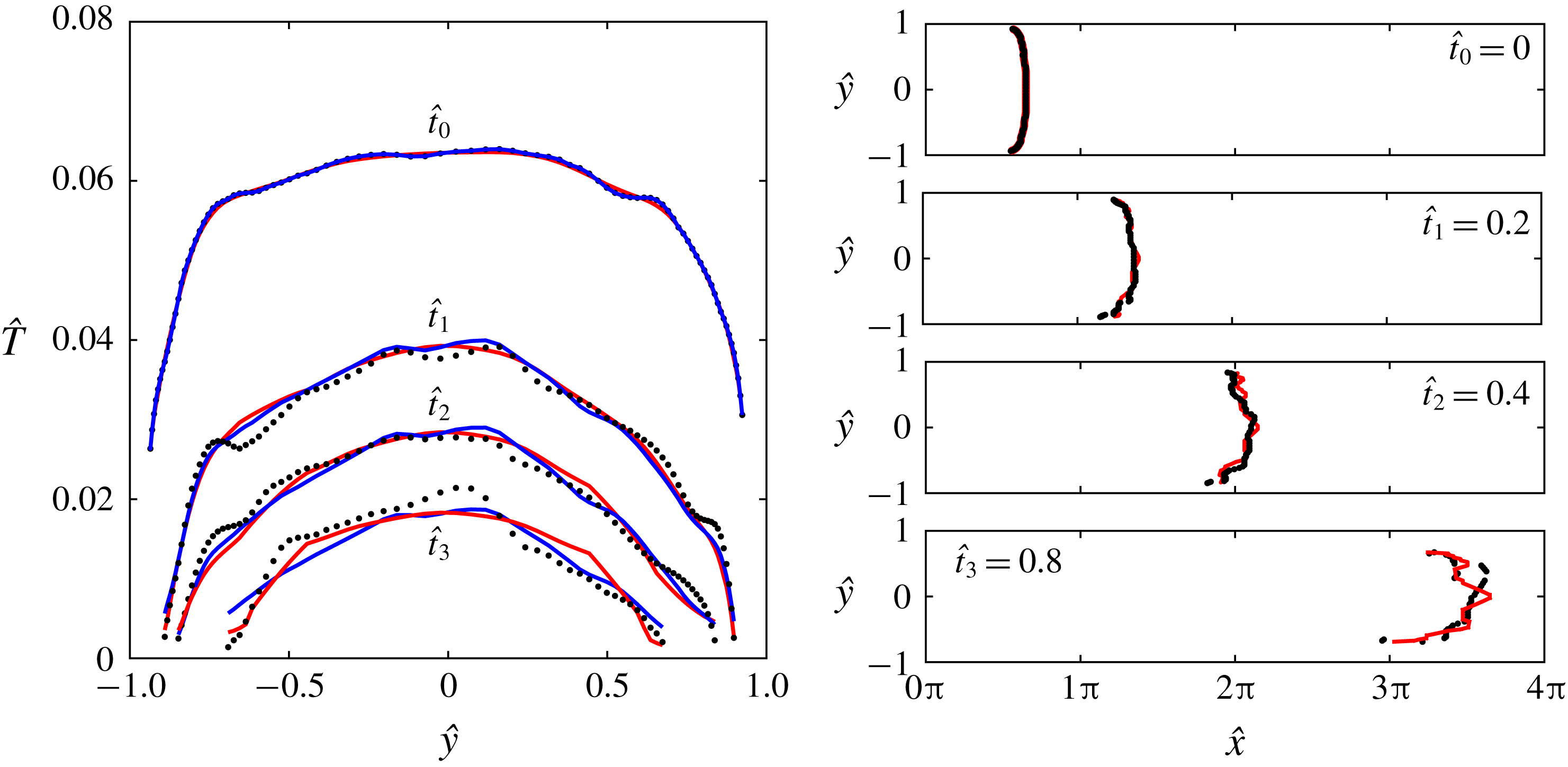
A visual comparison of the LOM and DNS solutions for the case of heat loss at the walls is shown in figure 11. Similar to the case of adiabatic walls, the position of the wave from the LOM is in good agreement with the position from the DNS in figure 11(b). The solution shown in figure 11 has a one-to-one time correspondence with the solution shown in figure 10 for the case of adiabatic walls. The position of the wave from the two cases is the same, indicating that the wave fronts are advecting at the same speed. Thus, the wave speed has not been affected by the heat loss to the walls. The heat loss to the walls has, relative to the adiabatic wall case, simply accelerated the dissipation of the wave near the walls causing the amplitude to quickly fall to zero and the edges of the wave to vanish. In the left column of figure 11, the solution of the LOM equation (3.8b
) with piecewise and continuous
 $\unicode[STIX]{x1D6FD}$
gives a good approximation of the amplitude decay from the DNS.
Accuracy of the low-order model solution in the case of convective heat loss at the walls: ● DNS, —— (red) nonlinear low-order model using a piecewise
 $\unicode[STIX]{x1D6FD}({\hat{y}})$
, —— (blue) nonlinear low-order model using a continuous
 $\unicode[STIX]{x1D6FD}({\hat{y}})$
given by (3.7).
The need for a variable
 $\unicode[STIX]{x1D6FD}$
in (3.8b
) in the case of heat loss at the walls is depicted in figure 12, which shows the amplitude decay from the LOM when the same
 $\unicode[STIX]{x1D6FD}$
is used in (3.8b
) for all the streamwise cross-sections. The amplitude from the equation with
 $\unicode[STIX]{x1D6FD}=0.5$
shows better agreement with the amplitude from the DNS over the equations with
 $\unicode[STIX]{x1D6FD}=1$
and
 $\unicode[STIX]{x1D6FD}=2$
at the edges of the wave. On the other hand, the nonlinear equation with
 $\unicode[STIX]{x1D6FD}=2$
shows the best agreement with the amplitude from the DNS near the centre line. Between the near-centre-line and near-edge parts of the wave, the amplitude from the equation with
 $\unicode[STIX]{x1D6FD}=1$
makes for a gentle transition. Hence, unlike the adiabatic walls, the case for which
 $\unicode[STIX]{x1D6FD}=2$
could be used everywhere. In the case of heat loss at the walls it is clearly needed to use a piecewise
 $\unicode[STIX]{x1D6FD}$
over the channel cross-section.
Amplitude decay from the LOM when the same
 $\unicode[STIX]{x1D6FD}$
is used for all the streamwise cross-sections: ● DNS, —— (red) LOM with
 $\unicode[STIX]{x1D6FD}=0.5$
, —— (green) LOM with
 $\unicode[STIX]{x1D6FD}=1$
, —— (blue) LOM with
 $\unicode[STIX]{x1D6FD}=2$
.

In order to carry out a more detailed comparison of the LOM and DNS solutions there is a need to define quantitative measures or metrics of accuracy. Such metrics are also needed in § 5 to consistently evaluate the accuracy of the LOM in relation to the length of the DNS time series. There are two criteria that have to be met for the LOM and DNS solutions to be considered in good agreement. First, the residual between the states has to be small and secondly the way in which the states vary over the cross-section has to be similar. Thus, two metrics are needed, one to measure the residual and another to evaluate the correlation between the corresponding states from the LOM and the DNS.
The residual between the states
 $\hat{\unicode[STIX]{x1D6F7}}_{j}^{LOM}$
from the LOM and the states
 $\hat{\unicode[STIX]{x1D6F7}}_{j}^{DNS}$
from the DNS is averaged over the cross-section to give an overall residual. The average residual of the states is equivalent to the residual of the average states given by (4.1) as follows:
 $$\begin{eqnarray}\unicode[STIX]{x1D716}_{\langle \hat{\unicode[STIX]{x1D6F7}}_{j}\rangle _{A}}=\frac{\langle \hat{\unicode[STIX]{x1D6F7}}_{j}^{LOM}\rangle _{A}-\langle \hat{\unicode[STIX]{x1D6F7}}_{j}^{DNS}\rangle _{A}}{\langle \hat{\unicode[STIX]{x1D6F7}}_{j}^{DNS}\rangle _{A}},\end{eqnarray}$$
where
 $\unicode[STIX]{x1D716}_{\langle \hat{\unicode[STIX]{x1D6F7}}_{j}\rangle _{A}}$
is the residual of the average state
 $\langle \hat{\unicode[STIX]{x1D6F7}}_{j}\rangle _{A}$
over the channel cross-section. The average state
 $\langle \hat{\unicode[STIX]{x1D6F7}}_{j}\rangle _{A}$
is given by (4.2), where
 $NY$
is the number of grid nodes used in the wall-normal direction for the DNS:
 $$\begin{eqnarray}\langle \hat{\unicode[STIX]{x1D6F7}}_{j}\rangle _{A}=\frac{1}{NY-1}\mathop{\sum }_{n=1}^{NY-1}(\hat{\unicode[STIX]{x1D6F7}}_{j}{\hat{y}})_{n}.\end{eqnarray}$$
The residual given by (4.1) is normalised with respect to the average state from the DNS. Due to the equivalence of the average residual with the residual of the average states, henceforth, the average residual over the channel cross-section is referred to simply as the residual meaning the residual of the average states. The sign of the residual indicates if the average state from the LOM is larger (positive) or smaller (negative) than the corresponding average state from the DNS.
The correlation between the states
 $\hat{\unicode[STIX]{x1D6F7}}_{j}^{LOM}$
from the LOM and the states
 $\hat{\unicode[STIX]{x1D6F7}}_{j}^{DNS}$
from the DNS over the channel cross-section is measured with the Pearson correlation coefficient
 $r_{\hat{\unicode[STIX]{x1D6F7}}_{j}}$
given by (4.3) as follows:
 $$\begin{eqnarray}r_{\hat{\unicode[STIX]{x1D6F7}}_{j}}=\frac{\displaystyle \mathop{\sum }_{n=1}^{NY}(\hat{\unicode[STIX]{x1D6F7}}_{j}^{DNS}-\langle \hat{\unicode[STIX]{x1D6F7}}_{j}^{DNS}\rangle _{A})_{n}(\hat{\unicode[STIX]{x1D6F7}}_{j}^{LOM}-\langle \hat{\unicode[STIX]{x1D6F7}}_{j}^{LOM}\rangle _{A})_{n}}{\displaystyle \sqrt{\mathop{\sum }_{n=1}^{NY}(\hat{\unicode[STIX]{x1D6F7}}_{j}^{DNS}-\langle \hat{\unicode[STIX]{x1D6F7}}_{j}^{DNS}\rangle _{A})_{n}^{2}\mathop{\sum }_{j=1}^{NY}(\hat{\unicode[STIX]{x1D6F7}}_{j}^{LOM}-\langle \hat{\unicode[STIX]{x1D6F7}}_{j}^{LOM}\rangle _{A})_{n}^{2}}}.\end{eqnarray}$$
The correlation coefficient
 $r_{\hat{\unicode[STIX]{x1D6F7}}_{j}}=+1$
indicates that the state from the LOM and the corresponding state from the DNS are perfectly correlated and, thus, their respective profiles over the cross-section have the same trend. However, a Pearson correlation coefficient
 $r_{\hat{\unicode[STIX]{x1D6F7}}_{j}}=0$
indicates that the states are uncorrelated over the channel cross-section and thus, that their respective profiles over the channel cross-section have radically different trends.
Time series plots of the residual (a,b) and correlation (c,d) of corresponding states from the LOM and DNS with respect to time for the case of adiabatic walls (a,c) and heat loss at the walls (b,d): ▫
 $\hat{x}$
, ▪
 $\hat{T}$
when LOM uses piecewise
 $\unicode[STIX]{x1D6FD}({\hat{y}})$
, ◂
 $\hat{T}$
when LOM uses continuous
 $\unicode[STIX]{x1D6FD}({\hat{y}})$
.

Time series plots of the metrics
 $\unicode[STIX]{x1D716}_{\langle \hat{\unicode[STIX]{x1D6F7}}_{j}\rangle _{A}}$
and
 $r_{\hat{\unicode[STIX]{x1D6F7}}_{j}}$
defined above are shown in figure 13(a,c) for the case of adiabatic walls and in figure 13(b,d) for the case of convective heat loss at the walls. The metrics for amplitude in the case of convective heat loss at the walls, in figure 13(b,d), are shown for the cases of the LOM using a piecewise and a continuous
 $\unicode[STIX]{x1D6FD}({\hat{y}})$
. The metrics for the different cases of the
 $\unicode[STIX]{x1D6FD}({\hat{y}})$
are nearly identical. In figures 13(a) and 13(b), the residual is less than
 $\pm 10\,\%$
and
 $\pm 1\,\%$
at all times for the amplitude and position, respectively, in both cases of the thermal boundary condition. The small residuals for both amplitude and position keeps with the visual comparison in figures 10 and 11. The reason for the larger amplitude residual is explained by referring to figure 7 in § 3, which shows the fittings made to the DNS data in a streamwise cross-section near the channel centre line. In figure 7, the amplitude data from the DNS is more spread-out than the position data and this is why in figure 13(a,b) the residual of amplitude is larger than that of position. In figures 13(c) and 13(d), the correlation is near unity at all times for amplitude and position in the case of adiabatic walls. In the case of convective heat loss at the walls, the correlation of amplitude is near unity at all times and the correlation of position, although not near unity at all times, never falls below
 $0.8$
.
5 Prediction
The comparison of the model and simulation results in § 4 is made using the entire length of the DNS time series to determine the model parameters. The good agreement observed between the states from the LOM and the DNS confirms that the LOM has been formulated correctly. Using shorter DNS time series to estimate the model parameters will diminish the accuracy of the LOM because the fittings that are made to the DNS data will, in such a case, be made to DNS data that does not cover the complete dynamical behaviour of the system. A minimum length of the DNS time series must exist below which the LOM does not predict, with an acceptable accuracy, the position and amplitude of the entropy wave beyond the range covered by the DNS time series used to estimate its parameters. In order to determine the minimum length of the DNS time series, the LOM parameters are estimated using progressively longer DNS time series and the accuracy of the LOM is evaluated relative to the length of the time series. The expectation is that the accuracy should approach an asymptotic limit as the length of the time series is increased from the minimum length needed for a first estimate of the model parameters to the full length of the DNS time series, which covers the entire dynamical behaviour.
For each length of the DNS time series the accuracy of the LOM is evaluated with use of the metrics defined in § 4. However, for DNS time series of any length the metrics are time-dependent because at every new time step the states from the LOM and DNS change and so does the accuracy of the LOM (see figure 13). Hence, the time-average of the absolute metrics (
 $\langle |\unicode[STIX]{x1D716}_{\langle \hat{\unicode[STIX]{x1D6F7}}_{j}\rangle _{A}}|\rangle _{t}$
,
 $\langle |r_{\hat{\unicode[STIX]{x1D6F7}}_{j}}|\rangle _{t}$
) is taken as a measure of the overall accuracy of the LOM for a given length of the DNS time series. The absolute value of the metrics is taken because a positive and negative residual or correlation coefficient would cancel out when averaged and thus, the average of non-absolute metrics would give wrong indications about the LOM accuracy.
Plots of the time-averaged metrics with respect to the length of the DNS time series used to estimate the parameters of the LOM are shown in figure 14(a,c) for the case of adiabatic walls and in figure 14(b,d) for the case of convective heat loss at the walls. The metrics for amplitude in the case of convective heat loss at the walls, in figure 14(b,d), are shown for the cases of the LOM using a piecewise and a continuous
 $\unicode[STIX]{x1D6FD}({\hat{y}})$
. In figure 14(a–d), the
 $0\,\%$
DNS data corresponds to fully developed turbulent flow before the addition of the entropy wave to the flow. Further, the initial
 $12.5\,\%$
of the DNS data (shaded region in the plots of figure 14) is the data obtained during the time taken to add the entropy wave. This initial DNS data is not used when formulating the LOM for two reasons. First, the current study is concerned with the advection of an entropy wave and not with its generation. Second, the existence of sharp temperature gradients in the flow during the addition of the entropy wave require higher-order terms to be included in the LOM equations. Nevertheless, the initial
 $12.5\,\%$
of the DNS time series is shown in the plots of figure 14 for completeness.
Plots of the time-averaged residual (a,b) and time-averaged correlation (c,d) of corresponding states from the LOM and DNS with respect to the length of the DNS time series used to formulate the LOM for the case of adiabatic walls (a,c) and heat loss at the walls (b,d): ▫
 $\hat{x}$
, ▪
 $\hat{T}$
when LOM uses piecewise
 $\unicode[STIX]{x1D6FD}({\hat{y}})$
, ◂
 $\hat{T}$
when LOM uses continuous
 $\unicode[STIX]{x1D6FD}({\hat{y}})$
.

In the case of adiabatic walls, in figure 14(a), the residual in amplitude is large for short DNS time series because there is insufficient DNS data for a good estimate of the LOM parameters and it reaches the asymptotic limit of
 ${\approx}2\,\%$
at
 ${\approx}25\,\%$
of the DNS data. As explained above, the first
 $12.5\,\%$
of the DNS data (shaded region in the plots of figure 14) is not used for the estimation of the LOM parameters and thus, the effective length of the DNS time series at
 $25\,\%$
is
 $12.5\,\%$
of the trace. The residual in position never exceeds
 $2\,\%$
because the wave speed is nearly equal to the flow speed (see § 3). The correlation in amplitude and position is very close to unity even for short DNS time series. The correlation of position is expected to be close to unity even for short DNS time series for the same reason as the residual is expected to be small. On the other hand, the close to unity correlation of amplitude for short DNS time series is not anticipated. This is an indication that the large residual in amplitude for short DNS time series is uniform over the channel cross-section at all times and hence, the amplitude remains correlated.
Accuracy of the low-order model solution in the case of adiabatic walls, where the model parameters are determined using
 $12.5\,\%$
of the full length of the DNS time series: ● DNS, —— (red) nonlinear low-order model.

In the case of convective heat loss at the walls, in figure 14(b), the residual in amplitude for both cases of
 $\unicode[STIX]{x1D6FD}({\hat{y}})$
and the residual in position are similar to the case of adiabatic walls. That is, the residual in amplitude is large for short DNS time series and reaches the asymptotic limit of
 ${\approx}2\,\%$
for the model parameters estimated using only
 ${\approx}12.5\,\%$
of the full length of the DNS time series. Further, the residual in position is approximately steady below
 $2\,\%$
. The correlation in amplitude and position is very close to unity irrespective of the length of the DNS time series just as in the case of adiabatic walls. The correlation of the amplitude from the LOM with a continuous
 $\unicode[STIX]{x1D6FD}({\hat{y}})$
is only marginally larger than that of the amplitude from the LOM with a piecewise
 $\unicode[STIX]{x1D6FD}({\hat{y}})$
.
The accuracy of the formulated LOM is acceptable only when the residual of the states is low and correlation of the states over the channel cross-section is close to unity. The error in the prediction of the LOM is minimum when at least
 $12.5\,\%$
of the full length of the DNS time series is used; for the adiabatic and heat transferring cases. This is visually confirmed in figures 15 and 16, which show a comparison of the LOM and DNS solutions when the model parameters are determined using only one-eighth of the full length of the DNS time series. Figures 15 and 16 show the comparison for the cases of adiabatic walls and convective heat loss at the walls, respectively. For the case of convective heat loss at the walls in figure 16, the solution of the LOM is shown for both the piecewise and continuous
 $\unicode[STIX]{x1D6FD}({\hat{y}})$
cases. The amplitude distribution from the LOM in the case of continuous
 $\unicode[STIX]{x1D6FD}({\hat{y}})$
is more wrinkled than in the case of piecewise
 $\unicode[STIX]{x1D6FD}({\hat{y}})$
. This is because
 $\unicode[STIX]{x1D6FD}({\hat{y}})$
is the order of the fit being made to the
 $(\hat{T},\dot{\hat{T}})$
data points in each streamwise cross-section. The fitting error depends on the order of the fit that varies continuously over the channel cross-section, therefore the fitting error introduces a variability that manifests in the model solution. The wrinkling is not so apparent in figure 11, where the entire DNS dataset is used to make the fittings, because the fitting error is minimised by the large dataset. Nonetheless, the wrinkling of the amplitude distribution is due to very small variations over the channel cross-section. Similarly to the comparisons shown in figures 10 and 11, when the full length of the DNS time series is used to determine the model parameters, the LOM and DNS solutions are in good agreement even when only one-eighth of the DNS time series is used. Therefore, an LOM of acceptable accuracy can be estimated by knowing in advance only one-eighth of the complete evolution of the entropy wave.
Accuracy of the low-order model solution in the case of convective heat loss at the walls, where the model parameters are determined using
 $12.5\,\%$
of the full length of the DNS time series: ● DNS, —— (red) nonlinear low-order model using a piecewise
 $\unicode[STIX]{x1D6FD}({\hat{y}})$
, —— (blue) nonlinear low-order model using a continuous
 $\unicode[STIX]{x1D6FD}({\hat{y}})$
given by (3.7).

The low-order model has also been applied to data from a Reynolds-averaged Navier–Stokes (RANS) calculation, resulting in a performance consistent with that shown for the DNS data. These results are shown in appendix B. It is observed that the model calibrated with RANS data, can accurately predict the shape and maximum amplitude of entropy waves simulated by DNS. However, accurate prediction of the wave amplitude across the entire channel cross-section, requires calibration with highly precise data. It is important to note that the methodology, although currently applied to simulation data, could equally be applied to experimental data. In those cases where additional flow features related to combustor flows are present, such as swirl and chemical reactions, it is expected that the formulated system of equations could have a different form than that found in the current work.
6 Conclusions
Unlike modelling approaches in the literature on advecting entropy perturbations, in the present study the perturbations have been given a more realistic representation whereby the entropy wave has a variable shape and amplitude. Doing so has enabled the low-order modelling of the advecting entropy wave by considering it as a stand-alone dynamical system that has two states, namely position and amplitude. Time series of the position and amplitude of an advecting entropy wave in a fully developed turbulent channel flow were first generated by conducting DNS. These time series were then used to formulate and subsequently validate the proposed low-order model through a rigorous and novel methodology. In the process, findings emerged in support of, and in opposition to, the main assumptions made by the conventional models of advecting entropy waves. These include advection of the wave at the isothermal flow velocity and linearity of the dynamics governing the decay of the wave amplitude. Both assumptions are made routinely and are based on the case of a wave of small amplitude without any prior proof of what constitutes a small amplitude.
In support of the first assumption, it was quantitatively confirmed, from the DNS data, that an entropy wave with an initial amplitude of
 $10\,\%$
of the base flow temperature advects at the local flow velocity. Regarding the second assumption, the present study has found opposing evidence. The differential equation formulated for amplitude in the proposed low-order model is nonlinear. Further, the present study showed that the linear approximation is only strictly reliable for the waves with amplitude smaller than
 $2\,\%$
of the base flow temperature. The linear differential equation underestimates the amplitude of the wave during the final stages of the advection when the wave is near the combustor exit nozzle. However, the proposed low-order model shows that a nonlinear differential equation predicts the amplitude of the wave with much higher accuracy.
The developed model, similar to the existing low-order models of advecting entropy waves, gives a wave that advects at the flow velocity. Yet, it significantly improves on the morphology of the evolving wave, which is non-uniform in both position and amplitude. Further, it improves on the characterisation of the amplitude decay by using a nonlinear differential equation, which allows for the wave annihilation to be predicted. Importantly, the case specific parameters of the proposed model can be estimated from limited numerical or experimental data that cover, at most, only
 $12.5\,\%$
of the complete trace of wave advection. This, together with the fact that the model equations are amenable to analytical solution, makes the developed model suitable for integration into active control systems as a constituent part of thermoacoustic network models. The approach is also consistent with the current simulation trends in which high-fidelity modelling of the reactive region is combined with a simplified aero-acoustic model, applied to the rest of the combustor. This is because the high-order modelling of the near-flame region, wherein entropy waves are generated and start advecting, is sufficient for the development of an LOM that can accurately predict the wave evolution. Finally, the model is also compatible with MIMO model architectures as the logical next step towards the development of better thermoacoustic models.
Acknowledgements
This work was supported by the UK Engineering and Physical Sciences Research Council (EPSRC) grant EP/M508056/1. Furthermore, this work used the EPSRC funded HPC centres Cirrus (https://www.epcc.ed.ac.uk/cirrus) and ARCHIE-WeSt (www.archie-west.ac.uk). ThelatterfacilitywasfundedbyEPSRCgrantEP/K000586/1. The raw data of this work are available from the University of Glasgow’s Enlighten: Research Data repository at http://dx.doi.org/10.5525/gla.researchdata.868.
Appendix A. Akaike information criterion
The likelihood or
 $AIC_{i}$
value that fit-type
 $i$
is the best approximation is given by (A 1) as follows:
 $$\begin{eqnarray}AIC_{i}=N\ln (RSS/N)+2K+\frac{2K(K+1)}{N-(K+1)},\end{eqnarray}$$
where
 $N$
is the number of data points,
 $RSS$
is the residual sum of squares, and
 $K$
(unity in the current work) is the number of parameters in the fit type.
The relative likelihood of fit type
 $i$
is
 $\unicode[STIX]{x1D6E5}_{i}$
defined by (A 2) as follows:
 $$\begin{eqnarray}\unicode[STIX]{x1D6E5}_{i}=AIC_{i}-\min (AIC_{i}),\end{eqnarray}$$
The normalised relative likelihood
 $w_{i}$
(known as the Akaike weight) is given by (A 3) as follows:
 $$\begin{eqnarray}\displaystyle & \displaystyle w_{i}=\frac{\exp (-{\textstyle \frac{1}{2}}\unicode[STIX]{x1D6E5}_{i})}{\displaystyle \mathop{\sum }_{i=1}^{N_{fits}}\exp (-{\textstyle \frac{1}{2}}\unicode[STIX]{x1D6E5}_{i})}. & \displaystyle\end{eqnarray}$$
The Akaike weight of each of the fits shown in figure 8 is shown in figure 17 for all the streamwise cross-sections. For example, very close to the walls, (
 ${\hat{y}}\approx \pm 1$
), the
 $(\hat{T},\dot{\hat{T}})$
data points are best approximated by the fit
 $\dot{\hat{T}}=\unicode[STIX]{x1D703}_{2}T^{0.5}$
because the Akaike weight of this fit type shown in figure 17(a) is very near to unity close to the walls and zero in all other streamwise cross-sections.
The regions of the flow in which the amplitude decays according to (a)
 $\dot{\hat{T}}=\unicode[STIX]{x1D703}_{2}T^{0.5}$
, (b)
 $\dot{\hat{T}}=\unicode[STIX]{x1D703}_{2}T$
and (c)
 $\dot{\hat{T}}=\unicode[STIX]{x1D703}_{2}T^{2}$
.

The model parameters (a)
 $\unicode[STIX]{x1D703}_{1}$
and (b)
 $\unicode[STIX]{x1D703}_{2}$
, determined using data from simulations with different turbulence treatment: ▫, (red) DNS and ▫, (blue) RANS.

Appendix B. Calibration of low-order model with RANS data
The low-order model has also been calibrated with data from RANS calculations. The RANS calculations were performed with the ANSYS Fluent solver using a grid of
 $76\times 69\times 19$
nodes in the streamwise, wall-normal, and spanwise directions, respectively. The mean velocity profile was in close agreement with that obtained from the DNS.
Accuracy of the low-order model calibrated with RANS data and compared with DNS data for the case of adiabatic walls: ● DNS, ——, (red) low-order model calibrated with RANS data.

Accuracy of the low-order model calibrated and compared with RANS data for the case of adiabatic walls: ● RANS, ——, (blue) low-order model calibrated with partial RANS data, and ——, (red) low-order model calibrated with full RANS data.

The model parameters obtained from the RANS calculation are compared in figure 18 to those obtained from the DNS. There is a good agreement between RANS and DNS for the wave speed
 $\unicode[STIX]{x1D703}_{1}$
in figure 18(a). This is confirmed in figure 19 that compares the DNS result with that of the LOM that has been calibrated with the RANS data. Regardless of the dataset used for calibration, the wave shape is always predicted well. For the dissipation factor
 $\unicode[STIX]{x1D703}_{2}$
in figure 18(b) the agreement between RANS and DNS is good around the channel centre line. However, moving away from the channel centre line, the value of the dissipation factor from the RANS dataset is smaller than the value from the DNS. Therefore, while the amplitude of the wave in the core flow can still be predicted accurately as confirmed in figure 19, realistic amplitude predictions in the near wall regions requires calibration with highly precise DNS data. It follows that, regardless of the dataset used for model calibration, the low-order model can predict the maximum amplitude of the wave across the channel.
Figure 20 demonstrates that by calibrating the model with partial RANS data, the LOM is able to predict the full RANS results with very good accuracy. Hence, as already shown for the case of data from DNS, the model can predict the full evolution of the entropy wave from partial data, thus eliminating the need for a high-fidelity computation of the entire domain.



