1 Introduction
Considering how turbulence interacts with objects immersed in the fluid in one way (modifying the transport of the objects) and two way (how the objects modify the turbulence) has wide application. Both small (
 $D<\unicode[STIX]{x1D702}$
) and large (
 $D>\unicode[STIX]{x1D702}$
) are relevant, where
 $D$
stands for particle diameter and
 $\unicode[STIX]{x1D702}$
for Kolmogorov length scale, as well as considering whether the objects are deformable or not. Elghobashi (Reference Elghobashi2019) provides a review of computational methods for these problems and notes in his conclusion that ‘the experimental data needed to validate the DNS results are virtually nonexistent’. A key reason for this is the difficulty of obtaining a large enough volume of near-homogeneous isotropic turbulence (HIT) in a stationary frame within which the three-dimensional (3-D) motion of particles can be studied. We believe the facility presented here could also be used to understand the dispersion of inertial solid particles under background turbulence in a controlled environment, extending the recent work on the settling dynamics of large irregular particles in quiescent flow in Esteban, Shrimpton & Ganapathisubramani (Reference Esteban, Shrimpton and Ganapathisubramani2018) and Esteban, Shrimpton & Ganapathisubramani (Reference Esteban, Shrimpton and Ganapathisubramani2019) among others.
Turbulent flows encountered in nature and in engineering problems are usually not isotropic. In the absence of turbulence production, this type of turbulence decays over space and time. Therefore, the study of generation and decay of homogeneous anisotropic turbulence is of paramount importance in furthering the understanding of the physics of these flows. Despite being a ‘simple’ flow, the generation of homogeneous turbulence in the laboratory has been a matter of investigation over the past several decades. Most studies have attempted to generate homogeneous isotropic turbulence (HIT). Mean velocity gradients are generally needed for the production of turbulent kinetic energy (TKE) and they usually remain in the flow, introducing a certain degree of anisotropy. Various studies have attempted to reach the high Reynolds numbers that are desired so that the inertial and dissipation range of scales are sufficiently separated. Finally, most experiments and numerical simulations have been carried out for cases where the largest scales of the flow are smaller than the size of the facility (or the direct numerical simulations (DNS) box), and therefore confinement does not affect turbulence evolution.
In this study, we present experimental results on the decay of homogeneous anisotropic turbulence. We monitor the evolution of velocity fluctuations, dissipation and different length scales during the decaying process. We report changes in the decay power laws as the turbulence length scale starts to get affected by the size of the facility. To our knowledge, this is the first experimental study that presents these details in a temporally decaying spatially stationary flow. In the following sections, we present a review of the previous studies on generation and decay of homogeneous turbulence and identify the gaps that can be addressed through the present study.
1.1 Generation of homogeneous turbulence
The most common manner of generating turbulence in laboratories is by means of a steady flow passing through a grid or mesh. These flows can achieve relatively high Reynolds numbers when using active grids (Makita Reference Makita1991; Mydlarski & Warhaft Reference Mydlarski and Warhaft1996, Reference Mydlarski and Warhaft1998; Larssen & Devenport Reference Larssen and Devenport2011; Kang, Chester & Meneveau Reference Kang, Chester and Meneveau2003) or low-viscosity fluids (Kistler & Vrebalovich Reference Kistler and Vrebalovich1966; Bodenschatz et al.
Reference Bodenschatz, Bewley, Nobach, Sinhuber and Xu2014). In these scenarios, turbulence moves with the flow and is homogeneous and isotropic in planes parallel to the grid. However, turbulence generated with these methods exhibits anisotropy in the streamwise velocity component. To overcome this limitation, stationary turbulence has been widely investigated by using stirring devices during the last few decades. These methods use oscillating grids (McDougall Reference McDougall1979; De Silva & Fernando Reference De Silva and Fernando1994; McKenna & McGillis Reference McKenna and McGillis2004) or counter/contra-rotating disks separated by certain distance (Marie & Daviaud. Reference Marie and Daviaud2004; Volk, Odier & Pinton Reference Volk, Odier and Pinton2006; Blum et al.
Reference Blum, Bewley, Bodenschatz, Gibert, Gylfason, Mydlarski, Voth, Xu and Yeung2011). Although these methods have been improved with optimal mesh sizes, strokes and frequencies of the grid oscillation, the turbulence generated still suffers from large mean flows with
 $\bar{U}\approx 0.25u^{\prime }$
, where
 $\bar{U}$
stands for mean velocity and
 $u^{\prime }$
for root mean square of the velocity fluctuations. Furthermore, a mechanical system driven by a motor is needed for the grid motion. This makes it more difficult to build a large experimental set-up where high Reynolds numbers are desired.
Another interesting approach to generate HIT is the usage of loudspeakers symmetrically arranged in a three dimensional volume pointing towards the centre of the chamber (Hwang & Eaton Reference Hwang and Eaton2004; Webster, Brathwaite & Yen Reference Webster, Brathwaite and Yen2004; Warnaars, Hondzo & Carper Reference Warnaars, Hondzo and Carper2006; Lu et al. Reference Lu, Fugal, Nordsiek, Saw, Shaw and Yang2008; Goepfert et al. Reference Goepfert, Marie, Chareyron and Lance2010; Chang, Bewley & Bodenschatz Reference Chang, Bewley and Bodenschatz2012). The activation of the loudspeakers generate synthetic jets and induce vortex rings that encounter each other at the centre of the chamber. The quality of the turbulence reported using this approach is better than using oscillating grids, but the region of interest covers a small volume (for example, a 5 cm radius in Chang et al. (Reference Chang, Bewley and Bodenschatz2012)). Similarly, loudspeakers can be substituted by propellers as in Zimmermann et al. (Reference Zimmermann, Xu, Gasteuil, Bourgoin, Volk, Pinton and Bodenschatz2010) and Dou et al. (Reference Dou, Pecenak, Cao, Woodward, Liang and Meng2016), but the volume of interest remains a limitation for these systems.
A random jet array (RJA) is a relatively new approach to generate quasi-HIT with zero-mean flow (Variano, Bodenschatz & Cowen Reference Variano, Bodenschatz and Cowen2004; Lavertu, Mydlarski & Gaskin Reference Lavertu, Mydlarski and Gaskin2006; Variano & Cowen Reference Variano and Cowen2008; Delbos et al.
Reference Delbos, Weitbrecht, Bleninger, Grand, Chassaing, Lincot, Kerrec and Jirka2009; Khorsandi, Gaskin & Mydlarski Reference Khorsandi, Gaskin and Mydlarski2013). This device consists of a planar configuration of jets that are turned on and off, randomly and independently, to produce turbulence. The use of a single RJA creates a nearly homogeneous flow with turbulence decay in the direction normal to the plane of jets with negligible mean flow,
 $\bar{U}\approx 0.1u^{\prime }$
, (Variano & Cowen Reference Variano and Cowen2008). Additionally, the turbulence generated with this device is reported to have isotropy values of the same order of magnitude that in grid-generated wind tunnel turbulence (
 $u_{1}^{\prime }/u_{2}^{\prime }\approx 0.8-0.66$
) and relatively high Reynolds numbers (
 $Re_{\unicode[STIX]{x1D706}}\approx 314$
) (Variano & Cowen Reference Variano and Cowen2008).
Recently, in Bellani & Variano (Reference Bellani and Variano2013) two RJA were separated by a distance of 162 cm, and faced each other. They used the same firing algorithm as proposed for the case of a single RJA (Variano & Cowen Reference Variano and Cowen2008), resulting in a nearly HIT with a negligible mean flow at the middle region of the tank. At the same time, the isotropy was improved and was reported to be in the range of 0.95–0.99. They also obtained high Reynolds numbers (
 $Re_{\unicode[STIX]{x1D706}}\approx 334$
) and a large region of HIT of approximately
 $0.4\times 0.4\times 0.2~\text{m}^{3}$
.
Following a similar approach as in Bellani & Variano (Reference Bellani and Variano2013), Carter et al. (Reference Carter, Petersen, Amili and Coletti2016) presented a facility in air consisting of two planar arrays of quasi-synthetic jets (
 $256$
in total) creating the largest region of homogeneous turbulence to date. Contrary to what was found in Bellani & Variano (Reference Bellani and Variano2013), they observed anisotropy at large scales for all configurations tested.
1.2 Decay of homogeneous turbulence
Together with the generation of turbulence, the study of its natural decay has been a matter of debate. Von Karman & Howarth (Reference Von Karman and Howarth1938) derived the transport equation that connects the double and triple streamwise velocity correlation functions for temporally decaying HIT:
 $$\begin{eqnarray}\frac{\unicode[STIX]{x2202}B_{uu}}{\unicode[STIX]{x2202}t}+2\left(\frac{\unicode[STIX]{x2202}B_{uuu}}{\unicode[STIX]{x2202}r}+4\frac{B_{uuu}}{r}\right)=2\unicode[STIX]{x1D708}\left(\frac{\unicode[STIX]{x2202}^{2}B_{uuu}}{\unicode[STIX]{x2202}r^{2}}+\frac{4}{r}\frac{\unicode[STIX]{x2202}B_{uu}}{\unicode[STIX]{x2202}r}\right),\end{eqnarray}$$
where,
 $t$
is time,
 $r$
is the radial distance from a given point,
 $\unicode[STIX]{x1D708}$
is the kinematic viscosity,
 $B_{uu}$
is the double correlation and
 $B_{uuu}$
is the triple correlation of the
 $u$
velocity fluctuation.
Under certain assumptions, this transport equation can predict the decay of turbulence. The most common approach to solve this equation is to look for solutions for which the correlation functions remain self-preserving during the decay. Thus, double and triple correlation functions collapse when they are normalized using a single length scale and a single velocity scale. Dryden (Reference Dryden1943), Batchelor (Reference Batchelor1948) and Korneyev & Sedov (Reference Korneyev and Sedov1976) among others, investigated these type of solutions, leading to the commonly accepted power-law decay for the turbulent kinetic energy over time, which has the form:
 $$\begin{eqnarray}q^{2}\sim (t-t_{0})^{m},\end{eqnarray}$$
where
 $q^{2}=u_{1}^{\prime 2}+u_{2}^{\prime 2}+u_{3}^{\prime 2}$
is twice the turbulent kinetic energy,
 $m$
is the power-law exponent and
 $t_{0}$
the temporal virtual origin. Early values of
 $m$
obtained experimentally in Compte-Bellot & Corrsin (Reference Compte-Bellot and Corrsin1966) led to the present consensus that
 $m\leqslant -1$
. From later experimental studies, as in Uberoi & Wallis (Reference Uberoi and Wallis1967), Ling & Wang (Reference Ling and Wang1972) or el Hak & Corrsin (Reference el Hak and Corrsin1974), other
 $m$
values were obtained, ranging from
 $-1$
to
 $-1.75$
.
Wind tunnels equipped with conventional passive grids, fractal passive grids and active grids have been extensively used to investigate the decay of quasi-homogeneous turbulence along the streamwise direction of the wind tunnel test section. However, in all these experiments, the temporal decay of turbulence is modelled as a function of downstream distance invoking Taylor’s hypothesis (Taylor Reference Taylor1938). Lavoie, Djenidi & Antonia (Reference Lavoie, Djenidi and Antonia2007) investigated whether the initial conditions can affect the decay exponent
 $m$
of approximately homogeneous isotropic turbulence. They carried wind tunnel experiments with four different conventional passive grids and two test sections and did not find any significant effect of initial conditions on the decay exponent
 $m$
. However, experimental results obtained from multi-scale grids in Krogstad & Davidson (Reference Krogstad and Davidson2011) and further analysed in Valente & Vassilicos (Reference Valente and Vassilicos2012) showed that the decay of approximately homogeneous turbulence remains dependent on the inflow conditions far downstream from its generation. Therefore, the decay exponent
 $m$
becomes non-universal and changes when the turbulence-generating grid is modified (1.15–1.25), (Valente & Vassilicos Reference Valente and Vassilicos2012). They believe that multi-scale wake interactions in the near-field of the turbulence-generating grid remain in the flow very far downstream and are responsible for the change in the decay exponent. Similarly, Hearst & Lavoie (Reference Hearst and Lavoie2014) performed wind tunnel experiments with a square-fractal element grid at farther downstream locations than previous studies and showed that a classical power-law decay region exists with exponents
 $m=-1.37$
and
 $m=-1.39$
for Reynolds number based on the integral length scale
 $Re_{L}=65\,000$
and
 $Re_{L}=57\,000$
respectively. The decay in the near-field region (
 $x/L<20$
) also followed a power-law evolution but with much higher decay exponents
 $m\approx -2.79$
, being in accordance with results obtained in Valente & Vassilicos (Reference Valente and Vassilicos2011) for multi-scale grids.
Direct numerical simulations (DNS) of periodic three-dimensional box turbulence have been carried out to investigate the temporal decay of HIT. As in the experiments detailed above, DNS results also give a broad spread of
 $m$
values for homogeneous isotropic turbulence, as in Huang & Leonard (Reference Huang and Leonard1994), de Bruyn Kops & Riley (Reference de Bruyn Kops and Riley1998), Wray (Reference Wray1998), Antonia & Orlandi (Reference Antonia and Orlandi2004) or Burattini et al. (Reference Burattini, Lavoie, Agrawal, Djenidi and Antonia2006). More recently, Goto & Vassilicos (Reference Goto and Vassilicos2016) carried direct numerical simulations of decaying three-dimensional Navier–Stokes turbulence in a periodic box with values of Taylor-length-based Reynolds number (
 $Re_{\unicode[STIX]{x1D706}}=u^{\prime }\unicode[STIX]{x1D706}/\unicode[STIX]{x1D708}$
, where
 $\unicode[STIX]{x1D706}$
is the Taylor micro-scale) up to
 $300$
. They combined these results with grid-generated turbulence with
 $Re_{\unicode[STIX]{x1D706}}\approx 350$
to reveal the ‘non-equilibrium dissipation law’ for near-field regions. Among the features discovered, they found a critical time when the scaling of the turbulence dissipation changes from the one recently discovered in DNS of forced unsteady turbulence and in wind tunnel experiments (for near field) to the classical scaling proposed by Taylor (Reference Taylor1935) and Kolmogorov (Reference Kolmogorov1941) (for far field).
Similarly, Meldi (Reference Meldi2016) performed numerical calculations based on the eddy damped quasi-normal Markovian (EDQNM) model to investigate the signature of production mechanisms in isotropic turbulence. They showed that an exponential decay law can be observed if the intensity of the forcing is sufficiently strong to drive the turbulence dynamics and then the decay is followed by a classical power-law decay. These results are also in good agreement with Hurst & Vassilicos (Reference Hurst and Vassilicos2007), Mazellier & Vassilicos (Reference Mazellier and Vassilicos2010) and Meldi, Lejemble & Sagaut (Reference Meldi, Lejemble and Sagaut2014) who also observed the near-exponential turbulence decay. As exposed in Meldi (Reference Meldi2016), ‘while a power-law evolution of HIT statistical quantities is eventually reached for all the classes of turbulence decay investigated, exponential decay law can be initially observed’ since this is governed by the forcing time evolution. An interesting point is also revealed by Meldi (Reference Meldi2016) concerning the time-lasting effects of production mechanisms. They suggest that these effects can be significantly larger than the observation time in grid experiments. Therefore, other facilities for which Taylor’s hypothesis is not invoked, and data can be taken at later decay times, are of interest to investigate these phenomena.
1.3 Confinement effects on decay of homogeneous turbulence
Although many numerical calculations (DNS, EDQNM) investigate the evolution of HIT decay over time, most studies do not continue simulations when the box size becomes comparable to the integral length scale of the flow. This is because these studies want to avoid non-physical effects that result from meeting this condition in the presence of periodic boundary conditions. Thus, confinement effects due to wall interactions still represent a great challenge in the study of turbulence decay. This aspect is generally referred to as saturation and is very relevant for the analysis of the test case of HIT. When the turbulent flow is unbounded, the exponent leading the evolution of the turbulent kinetic energy, the energy dissipation rate, the integral length scale and the Reynolds number is determined by the turbulence production mechanisms/initial conditions. However, as the integral scale grows to the size of the box that contains the flow (simulation box size or facility cross-section) an increase of the decay exponent for the TKE and dissipation rate (
 $\unicode[STIX]{x1D716}$
) is expected (
 $m=-2$
and
 $m_{\unicode[STIX]{x1D716}}=-3$
), as introduced in Skrbek & Stalp (Reference Skrbek and Stalp2000) and further discussed in Touil, Bertoglio & Shao (Reference Touil, Bertoglio and Shao2002).
Works based on a spectral space approach connect the decay exponent with the energy distribution at very large scales; i.e. they express the decay exponent of the turbulent kinetic energy as a function of the slope (
 $\unicode[STIX]{x1D70E}$
) of the energy spectrum at very small wavenumber (
 $k$
). The most studied values are
 $\unicode[STIX]{x1D70E}=2$
and
 $\unicode[STIX]{x1D70E}=4$
, since they are related to the general conservation principles and are historically used invariant quantities. The former is related to conservation of the linear moment and the Birkhoff–Saffman invariant and is referred to as Saffman turbulence. The latter is associated with the conservation of angular momentum and the Loitsyansky invariant and is referred to as Batchelor turbulence. In Touil et al. (Reference Touil, Bertoglio and Shao2002), they compared results from DNS, large eddy simulations (LES) and the EDQNM model on the decay of isotropic turbulence in a finite domain. In order to do so, they introduced a low-wavenumber cutoff into the energy spectrum. They used a pseudo-spectral technique with the low-wavenumber cutoff imposed at
 $k=2\unicode[STIX]{x03C0}/d$
(
 $d$
being the size of the box) but otherwise behaving as
 $k^{4}$
(
 $\unicode[STIX]{x1D70E}=4$
) at small
 $k$
. An initial power-law decay was observed for all models tested with an exponent
 $m\approx -1.42$
in agreement with the analytical expression for the model spectrum introduced. Then, the decay exponent increased as the scales of the flow grew during the decay and once the flow was fully saturated a decay exponent
 $m=-2$
was observed.
On the other hand, most numerical investigations only explore the decay of HIT; yet the initial conditions in wind tunnel experiments are neither homogeneous nor isotropic, and they only become quasi-isotropic some distance downstream from the grid (i.e. far field of the grid). In Biferale et al. (Reference Biferale, Boffetta, Celani, Lanotte, Toschi and Vergassola2003), they carried out a numerical investigation for the decay of three-dimensional anisotropic turbulence. They found that both large and small scales begin to ‘isotropize’ after approximately one eddy turnover time (
 $t_{L}$
) and become fully isotropic (within statistical fluctuations) for
 $t>100t_{L}$
. However, small scales showed a much higher degree of isotropy than large scales.
To our best knowledge, the study of Hwang & Eaton (Reference Hwang and Eaton2004) is the only experimental study where a zero-mean flow facility has been used to investigate the effect of natural decaying turbulence. They generated stationary turbulence by using eight synthetic jet actuators on the corners of a cubic chamber. The integral length scale of the flow for forced turbulence was
 $L=56~\text{mm}$
, which corresponded to
 ${\approx}1/7$
of the size of the chamber. The relative size of the integral length scale in this set-up is in fact considered ‘too big’ for unbounded flows in classical DNS with a periodic box domain. Unsurprisingly, they found a power-law decay for the TKE in time with an exponent of
 $m=-1.86$
. They suggested a possible weak isotropy during the decay and the initial conditions to be responsible for the high value of
 $m$
. However, we believe the saturation effect might have played a crucial role during the decay.
1.4 Objectives of this study
Here, we present an experimental set-up that can directly observe the temporal decay of turbulence without invoking Taylor’s hypothesis. This consists of a modified version of the RJA proposed in Bellani & Variano (Reference Bellani and Variano2013). This allows us to generate homogeneous but anisotropic (to a certain degree) turbulence and to examine how the characteristics of this type of turbulence evolve over time as the turbulence decays. Moreover, as the turbulence decays, the scales of the flow grow and the integral length scale could become comparable to the facility size. Thus, our aim is twofold: first to investigate the evolution of anisotropic turbulence and second to determine if spatial confinement affects the decay as previously found in DNS studies.
In § 2 we describe the apparatus and techniques. In § 3 we investigate the quality of the turbulence generated for the ‘stationary’ state and report the main turbulent quantities estimated. In § 4 we investigate the evolution of anisotropic turbulence and report on the saturation effects and we conclude in § 5.
2 Experimental set-up and measurement technique
2.1 Facility description and firing protocol
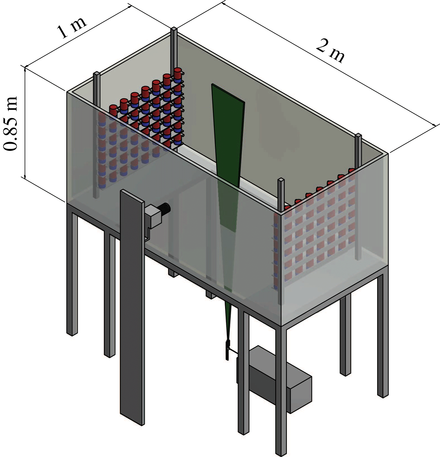
The experimental facility is an open glass (bottom and walls) and steel-framed tank of dimensions
 $200\times 85\times 100~\text{cm}^{3}$
. The origin of the coordinate system is at the centre of the tank,
 $x_{1}$
is oriented along the horizontal dimension of the tank (200 cm length),
 $x_{2}$
along the vertical dimension of the tank (85 cm length) and
 $x_{3}$
along the spanwise direction (100 cm length).
The structure holding the water tank is designed so that the centre region of the tank (
 $100\times 90~\text{cm}$
) is optically accessible from the bottom. The instantaneous velocity vector
 $\tilde{U} (x_{1},x_{2})$
is defined to be aligned with the
 $x_{1}$
and
 $x_{2}$
axes at the centre of the spanwise dimension. The tank is filled with tap water and is continuously filtered to 5
 $\unicode[STIX]{x03BC}$
m when experiments are not undertaken.
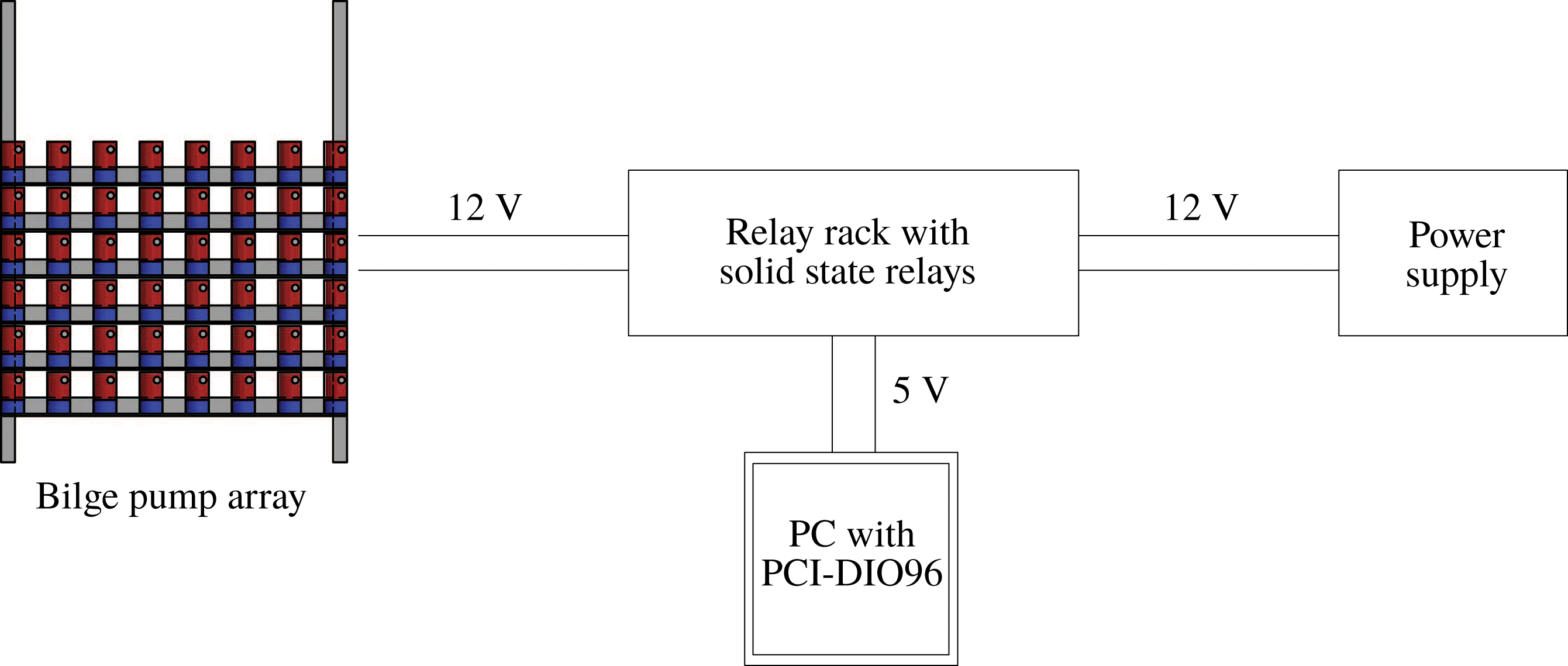
Turbulence is generated by two facing planes of randomly actuated jet arrays, in the same fashion as in Bellani & Variano (Reference Bellani and Variano2013). Each plane of jets contain
 $48$
bilge pumps (Rule 24, 360 GPH) arranged in a
 $8\times 6$
array as shown in figure 1. The pumps take in water radially at their base and discharge it axially via a cylindrical nozzle with 1.8 cm inner diameter. Each pump acts as a synthetic jet, in the sense that they only inject momentum to the system, since the pump intake and nozzle are contained within the same volume of fluid. The nozzle outlets are aligned so that they form a Cartesian grid with centre-to-centre distance (
 $M$
, as the mesh length of a wind tunnel grid) of 10 cm in both horizontal and vertical directions. The temperature of the water while the facility is in operation was monitored and found to change marginally during the experimental runs. Each plane of bilge pumps (
 $48$
units) is connected to a solid state relay rack SSR-RACK48 equipped with quad-core relays SSR-4-ODC-05. Each relay closes a circuit that supplies 12 V and up to 3 A to any specific pump. The relays are triggered by transistor-transistor logic (TTL) signals from a Measurement Computing 96 channel digital output card (PCI-DIO96H) controlled by MATLAB. The firing algorithm we employ to force turbulence is the ‘Sunbathing algorithm’ originally proposed in Variano & Cowen (Reference Variano and Cowen2008), and latter investigated in Bellani & Variano (Reference Bellani and Variano2013) and Carter et al. (Reference Carter, Petersen, Amili and Coletti2016) among others. This forcing algorithm pertains to the family of stochastic forcing in both space and time. The time durations for each pump to be active or inactive are picked from Gaussian distributions with a characteristic mean and standard deviation for the ‘on’ and ‘off’ times. The normal distribution parameters are
 $(\unicode[STIX]{x1D707}_{on},\unicode[STIX]{x1D70E}_{on})=(3,1)~\text{s}$
, and
 $(\unicode[STIX]{x1D707}_{off},\unicode[STIX]{x1D70E}_{off})=(21,7)~\text{s}$
, which results in an average of
 $\unicode[STIX]{x1D719}=12.5\,\%$
of the pumps being ‘on’ at any given time. This algorithm was identified in the literature to provide the best turbulence quality in terms of homogeneity and isotropy. The average time for which the tank is operated under the same conditions (
 $\unicode[STIX]{x1D70F}_{f}=\unicode[STIX]{x1D719}\unicode[STIX]{x1D707}_{on}$
) is smaller than the elapse time between subsequent image samples (2 s) and therefore these are uncorrelated in time with the forcing scheme.
Sketch of a bilge pump array (RJA) connection to the SSR-RACK48, PCI-DIO96H and power supply.

2.2 Particle image velocimetry (PIV) measurements
Sketch of the water tank equipped with a co-planar arrangement of RJAs and the PIV set-up.

All measurements are performed along the
 $x_{1}{-}x_{2}$
symmetry plane, whose origin is at the centre of the water tank, as illustrated in figure 2. The flow is seeded with
 $50~\unicode[STIX]{x03BC}\text{m}$
polycrystalline particles. The seeding is mixed in the water tank prior to the experimental run while the jets are randomly actuated to assure an even mixture. The imaging system consist of a dual-pulse Nd:YAG laser (Bernouilli, 532 nm wavelength,
 $100~\text{mJ}~\text{pulse}^{-1}$
) synchronized with a CCD camera (Imperx
 $6600\times 4400~\text{px}$
,
 $5.5~\unicode[STIX]{x03BC}\text{m}~\text{px}$
size). The laser beam is shaped into a 3 mm sheet (with 1.5 mm of full width at half-maximum) via a combination of two spherical and one cylindrical lenses and directed vertically through the glass bottom of the tank. We use a Sigma lens of 110 mm, leading to a magnification factor of
 ${\approx}38~\text{px}~\text{mm}^{-1}$
and a field of view of
 $110\times 160~\text{mm}$
in the
 $x_{1}{-}x_{2}$
symmetry plane. An external synchronizer that allows variable pulse separation (
 $dt$
) is used to trigger the laser and camera system. The pulse separation time is chosen such that the average particle displacement is limited to 4–6 px. This low particle displacement is necessary to reduce out-of-plane loss of particles. The velocity fields are obtained using DaVis, with a sliding minimum intensity background subtracted from every image prior to the velocity processing. The image processing is done by using an iterative cross-correlation algorithm with one refinement and three passes (
 $32\times 32~\text{px}$
first pass and
 $24\times 24~\text{px}$
second and third pass) with a 75 % overlap. A Gaussian fitting function is used to determine sub-pixel displacement. The sampling frequency is 0.5 Hz, and we acquire 1250 pair of images for stationary forced turbulence.
Vector validation is based on signal-to-noise ratio and deviation from the median of the neighbouring vectors. Non-valid vectors are less than 4 % and are later interpolated from neighbouring vectors.
The random error on the statistics associated with the finite number of samples is smaller than
 $3\,\%$
for the mean and for the root mean square velocity fluctuations, based on a
 $95\,\%$
confidence level. We choose the sampling frequency of 0.5 Hz to guarantee full statistical independence of the realizations, given that the typical large eddy turnover time is
 $t_{L}\approx 1.5~\text{s}$
. In the presentation of the results, the velocity measured
 $\tilde{U} _{i}$
is decomposed into the spatial averaged velocity
 $U_{i}$
and velocity fluctuations
 $u_{i}$
, such that
 $\tilde{U} _{i}=U_{i}+u_{i}$
. The prime symbol stands for root mean square of the velocity fluctuations, defined as
 $u_{i}^{\prime }=\sqrt{\langle \overline{u_{i}^{2}}\rangle }$
; and the operators
 $\bar{\cdot }$
and
 $\langle \cdot \rangle$
indicate ensemble average and spatial average, respectively. The sub-indices 1 and 2 stand for the velocity components along the horizontal and vertical direction, respectively.
3 Results for stationary turbulence
3.1 Single-point statistics and flow quality
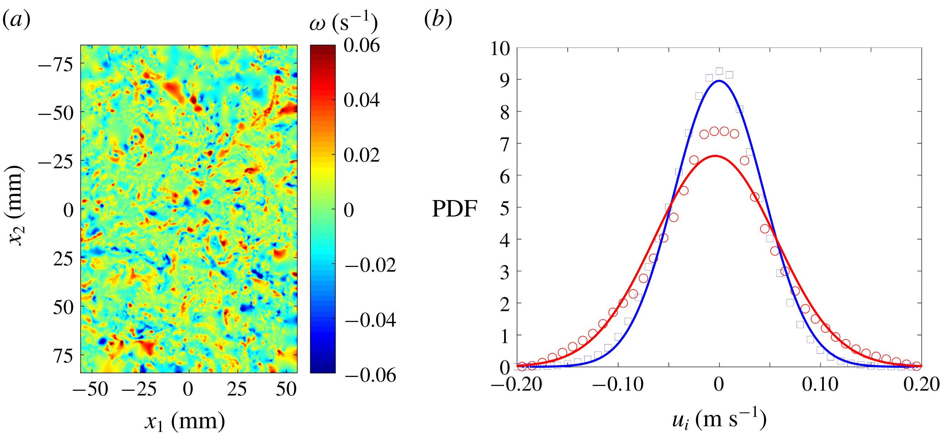
The statistics of the ‘Sunbathing algorithm’ for stationary turbulence are investigated using two-dimensional PIV data, as previously mentioned. Figure 3(a) shows a snapshot of the turbulent flow at the centre of the water tank, visualized by means of out-of-plane vorticity. The probability density function of the horizontal and vertical velocity fluctuations (
 $u_{i}$
) are shown in figure 3(b) (
 $1250$
pairs of images). The ensemble average of the in-plane mean velocity yields a value of
 $(\bar{U}_{1},\bar{U}_{2})=(3.6,1.5)~\text{mm}~\text{s}^{-1}$
. This is one order of magnitude smaller than the velocity fluctuations and consistent with other results in the literature; (Bellani & Variano Reference Bellani and Variano2013; Carter et al.
Reference Carter, Petersen, Amili and Coletti2016).
Instantaneous realization of out-of-plane vorticity (a). Distribution of horizontal and vertical velocity fluctuations represented with circles and squares respectively. The solid lines represent the best fitted normal distribution (b).

These two quantities, mean and velocity fluctuations, are characterized by having a homogeneous distribution that spans all of the region investigated here.
The homogeneity deviation is used to evaluate the spatial variation of the root-mean-square (r.m.s.) velocity fluctuation as
 $$\begin{eqnarray}HD=\frac{2\unicode[STIX]{x1D70E}_{u}}{u^{\prime }}\end{eqnarray}$$
where
 $\unicode[STIX]{x1D70E}_{u}$
is the spatial standard deviation of the ensemble average of the velocity fluctuations (
 $\sqrt{\overline{u_{i}^{2}}}$
), whereas the factor
 $2$
warrants a 95 % confidence interval.
 $HD$
is less than
 $0.1$
, showing good flow homogeneity in the domain investigated.
Similarly, the mean flow factor is used to show the strength of the mean flow in relation to the velocity fluctuations;
 $$\begin{eqnarray}MFF=\frac{|\overline{U}|}{u^{\prime }}.\end{eqnarray}$$
This flow factor is 0.012 showing the low relative strength of the mean flow in relation to the velocity fluctuations.
The strain-rate factor compares the strain within the ensemble average of the velocity fluctuations with the strain in the fluctuating velocity field as:

where
 $\unicode[STIX]{x1D634}_{11}$
is the longitudinal component of the fluctuating strain-rate tensor
 $\unicode[STIX]{x1D634}_{ij}=(1/2)(\unicode[STIX]{x2202}u_{i}/\unicode[STIX]{x2202}x_{j}+\unicode[STIX]{x2202}u_{j}/\unicode[STIX]{x2202}x_{i})$
. The velocity gradient
 $\unicode[STIX]{x2202}\overline{u_{1}}/\unicode[STIX]{x2202}x_{1}$
is verified to be the largest among the measured components of the ensemble average velocity gradient tensor. Therefore, the value of
 $MSRF=0.043$
confirms the low level of mean flow strain compared with its fluctuating counterpart.
3.2 Multi-point statistics and flow scales
Two-point correlation functions are used to investigate turbulent integral length scales (
 $L_{ij}$
) and Taylor length scales (
 $\unicode[STIX]{x1D706}_{1}$
,
 $\unicode[STIX]{x1D706}_{2}$
). The normalized correlation function is defined as:
 $$\begin{eqnarray}\unicode[STIX]{x1D70C}_{ii}(\boldsymbol{r})=\langle \overline{u_{i}(\boldsymbol{x}+\boldsymbol{r})u_{i}(\boldsymbol{x})}\rangle /\langle \overline{u_{i}^{2}(\boldsymbol{x})}\rangle\end{eqnarray}$$
being independent of the position vector
 $\boldsymbol{x}$
for homogeneous turbulence. The integral length scale that characterizes the velocity fluctuations
 $u_{i}$
over separations aligned with the position vector
 $x_{j}$
is obtained as:
 $$\begin{eqnarray}L_{ij}=\int _{0}^{r_{0}}\unicode[STIX]{x1D70C}_{ii}(r_{j})\,\text{d}r,\end{eqnarray}$$
where
 $r_{j}$
represents the separation in the direction
 $x_{j}$
and
 $r_{0}$
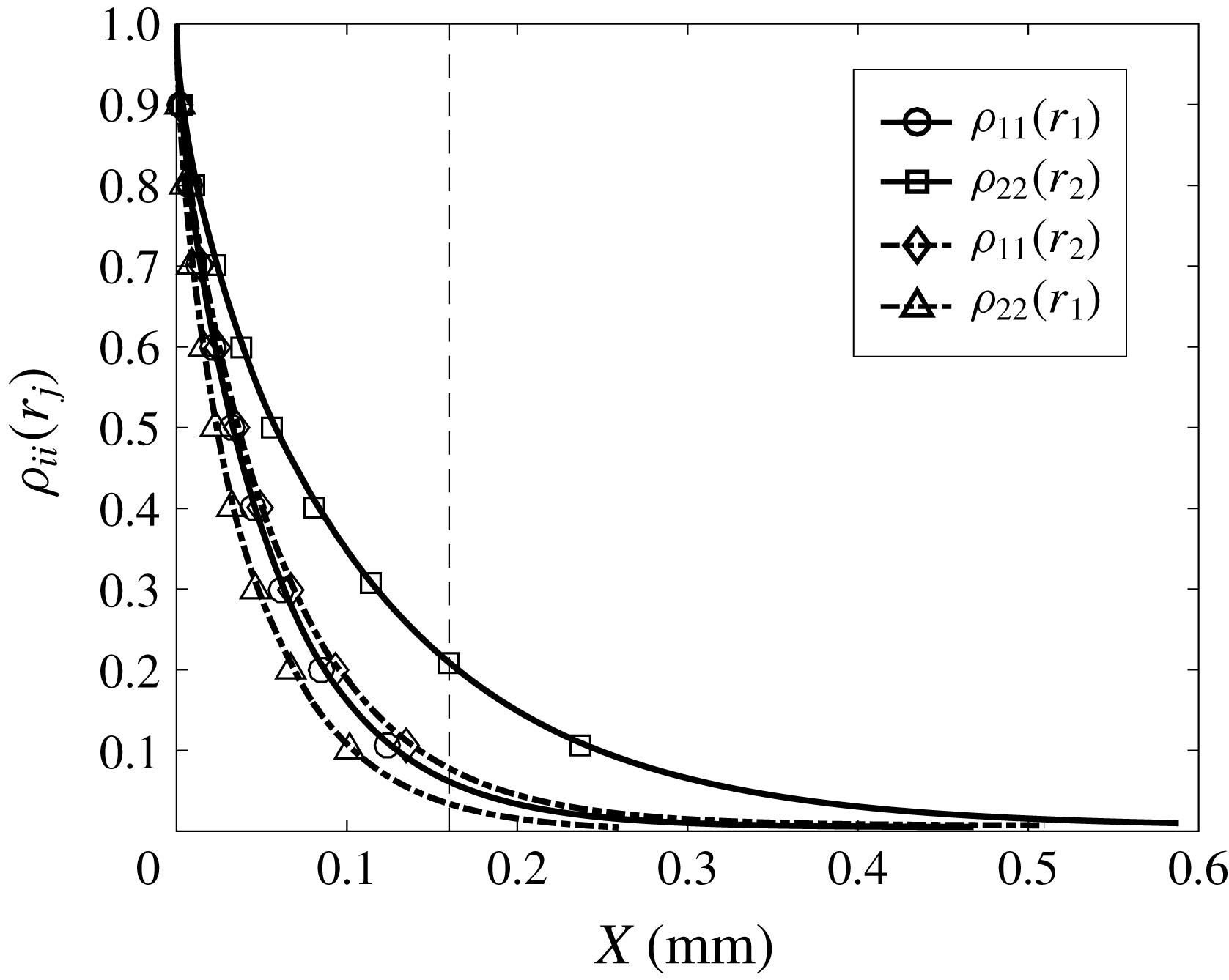
is the first zero crossing of the correlation function. The experimental data allow us the integration up to a distance of 16 cm. We extrapolate the tail of the correlation function using an exponential fit up to a value of
 $\unicode[STIX]{x1D70C}_{ii}(r_{j})=0.005$
and found an integral length scale
 $L_{11}\approx 9.1~\text{cm}$
for the horizontal velocity fluctuation along the longitudinal direction. This result shows that the correlation function from the experimental data only resolves the flow to distances
 $r_{1}<2L_{11}$
and therefore, this magnitude should be taken as an estimate. Figure 4 shows the correlation function of the horizontal and vertical component of the velocity fluctuations along the longitudinal and transverse direction, with the vertical broken line marking the start of the extrapolation region.
Longitudinal and transverse two-point correlation for the ‘Sunbathing algorithm’ firing scheme, where the vertical broken line shows the start of the extrapolation.

Table 1 shows that large scales have significant anisotropy, with an integral scale ratio
 $L_{11}/L_{22}\approx 1.6$
. There are several differences between the set-up presented here and the one in Bellani & Variano (Reference Bellani and Variano2013) that introduce large-scale anisotropy. The bilge pumps in Bellani & Variano (Reference Bellani and Variano2013) are mounted horizontally with a
 $90^{\circ }$
elbow attached to the original cylindrical nozzle of the pump. This increases the size of the orifice from
 $18$
to 21.9 mm and also modifies the components of the momentum introduced into the system, introducing strong secondary flows as detailed in Hellström et al. (Reference Hellström, Zlatinov, Cao and Smits2013). The size of the water tank in Bellani & Variano (Reference Bellani and Variano2013) is larger than the one presented here, they use mesh grids in front of the RJA and the working distance between RJAs is slightly larger. Similarly, we observed that the turbulence generated in their facility shows a relatively small mean velocity fluctuation and therefore Reynolds number compared with the one presented here. It is also interesting to note that the water pump flow rate is proportional to the current supplied and therefore, small differences in power supplies can lead to differences in the flow generated. In here, the power supplied to the water pumps was verified to give the maximum flow rate.
On the other hand, in the thorough study of Carter et al. (Reference Carter, Petersen, Amili and Coletti2016), they observed similar values of large-scale anisotropy as here and suggested that an excess of momentum on the horizontal direction was carried by their pressurized nozzles. They investigated the spacing between arrays of jets, the effect of passive grids and the spacing between working jets (
 $M$
) and found that the large-scale anisotropy was almost unaffected. Therefore, we believe the excess of horizontal momentum is also the cause of the large-scale imbalance in our facility.
Main turbulence statistics for the ‘Sunbathing algorithm’.

The Taylor length scale is obtained by fitting a parabola to the three first uncorrelated points of the correlation function (excluding the origin). Then, the crossing point of the parabola with the
 $x$
-axis defines the length of this turbulent scale, whereas the crossing of the parabola with the
 $y$
-axis defines the ‘true’ r.m.s. velocity and also gives a measure of the random noise introduced during the PIV processing (Adrian & Westerweel Reference Adrian and Westerweel2011), of
 ${\approx}5\,\%$
here.
To calculate the Kolmogorov scales of the flow, a reliable estimation of the turbulent kinetic energy dissipation rate is needed. To do so, first we evaluate the flow isotropy at small scales by comparing the velocity gradients of the two-dimensional PIV data after applying a Gaussian smoothing of
 $3\unicode[STIX]{x1D702}$
, as proposed in Ganapathisubramani, Lakshminarasimhan & Clemens (Reference Ganapathisubramani, Lakshminarasimhan and Clemens2007); i.e.
 $2(\unicode[STIX]{x2202}u_{i}/\unicode[STIX]{x2202}x_{i})=\unicode[STIX]{x2202}u_{i}/\unicode[STIX]{x2202}x_{j}$
for isotropic turbulence. We observe that for forced stationary turbulence, the ratio of longitudinal to transverse velocity derivatives does not correspond to isotropic turbulence. In contrast, we observe an average ratio of
 $1.3(\unicode[STIX]{x2202}u_{i}/\unicode[STIX]{x2202}x_{i})\approx \unicode[STIX]{x2202}u_{i}/\unicode[STIX]{x2202}x_{j}$
for both velocity components; i.e.
 $i\neq j$
. Therefore, based on this result and the axisymmetric nature of the jet forcing around the
 $x$
-axis reported in previous studies (Variano & Cowen Reference Variano and Cowen2008; Bellani & Variano Reference Bellani and Variano2013; Alvarado, Mydlarski & Gaskin Reference Alvarado, Mydlarski and Gaskin2016; Carter et al.
Reference Carter, Petersen, Amili and Coletti2016), we estimate the TKE dissipation rate following the equation derived in George & Hussein (Reference George and Hussein1991) for local axisymmetric turbulence,
 $$\begin{eqnarray}\unicode[STIX]{x1D716}=\unicode[STIX]{x1D708}[-\langle \overline{\unicode[STIX]{x1D634}_{11}^{2}}\rangle +2\langle \overline{\unicode[STIX]{x1D634}_{12}^{2}}\rangle +2\langle \overline{\unicode[STIX]{x1D634}_{21}^{2}}\rangle +8\langle \overline{\unicode[STIX]{x1D634}_{22}^{2}}\rangle ]\end{eqnarray}$$
where
 $\unicode[STIX]{x1D634}_{ij}$
is the fluctuating strain rate. The presence of noise in high-resolution PIV data rapidly increases the error in the dissipation rate leading to an overestimation of this parameter, as demonstrated by Saarenrinne & Piirto (Reference Saarenrinne and Piirto2000). The PIV data we use resolve all spatial scales of the flow, with a vector spacing
 $\unicode[STIX]{x0394}x\approx 0.9\unicode[STIX]{x1D702}$
. However, the strong out-of-plane motion inherent of this facility increases the error associated with random experimental noise and consequently, the dissipation rate for which the velocity gradients are calculated will be affected, as investigated in Tanaka & Eaton (Reference Tanaka and Eaton2007) for sub-Kolmogorov PIV resolution and in de Jong et al. (Reference de Jong, Cao, Woodward, Salazar, Collins and Meng2009) or Buxton, Laizet & Ganapathisubramani (Reference Buxton, Laizet and Ganapathisubramani2011) for
 $\unicode[STIX]{x0394}x>\unicode[STIX]{x1D702}$
. To reduce the effect of noise in the direct estimation of the TKE dissipation rate, we apply a Gaussian filter to the velocity field with a kernel size
 $3\unicode[STIX]{x1D702}$
. This filter size in space, introduced in Ganapathisubramani et al. (Reference Ganapathisubramani, Lakshminarasimhan and Clemens2007), is equivalent to a frequency filter of
 $1.75f_{\unicode[STIX]{x1D702}}$
for point measurement techniques, identified in Antonia, Satyaprakash & Hussain (Reference Antonia, Satyaprakash and Hussain1982) as the optimum setting to capture velocity gradients accurately. The dissipation estimate can be also based on the scaling argument
 $\unicode[STIX]{x1D716}=C_{\unicode[STIX]{x1D716}}u^{\prime 3}/L_{11}$
, where
 $C_{\unicode[STIX]{x1D716}}$
is a constant of order unity (Sreenivasan Reference Sreenivasan1984). Later results from DNS of forced homogeneous isotropic turbulence in Sreenivasan (Reference Sreenivasan1998) and Burattini, Lavoie & Antonia (Reference Burattini, Lavoie and Antonia2005) found the value for
 $C_{\unicode[STIX]{x1D716}}$
(in their paper, it is represented as
 $A$
) to be
 ${\approx}0.5$
for
 $Re_{\unicode[STIX]{x1D706}}>200$
. Here, we use
 $C_{\unicode[STIX]{x1D716}}=0.5$
to estimate the dissipation rate in table 2, although this approach seems to underestimate TKE dissipation rate severely. The results obtained from the scaling argument and direct measure of the TKE dissipation rate are compared against the value obtained from the structure function fitting method. This is based on the relationship between the velocity structure functions and the dissipation rate invoking Kolmogorov’s second similarity hypothesis (Kolmogorov Reference Kolmogorov1941) in the inertial sub-range. Here, we use compensated second-order structure functions, as detailed in appendix A. The measure of dissipation rate with this method was considered in de Jong et al. (Reference de Jong, Cao, Woodward, Salazar, Collins and Meng2009) as the most robust indirect method and has been extensively used in zero-mean flow facilities, (Bellani & Variano Reference Bellani and Variano2013; Carter et al.
Reference Carter, Petersen, Amili and Coletti2016).
Dissipation rate estimates. The direct estimate of
 $\unicode[STIX]{x1D716}$
from the unfiltered and filtered data comes from (3.6); SFT stands for structure function fit. Dissipation rate in
 $(\text{m}^{2}\text{s}^{-3}\times 10^{-3})$
.

The TKE dissipation rate estimates obtained from the longitudinal structure functions from both velocity components (figure 15 in appendix A) agree within a few per cent, giving a TKE dissipation rate of
 $\unicode[STIX]{x1D716}\approx 1.4\times 10^{-3}~\text{m}^{2}~\text{s}^{-3}$
. Furthermore, this value is in good agreement with the dissipation estimate obtained from (3.6) after applying a Gaussian spatial filter to the velocity fields of
 ${\approx}3\unicode[STIX]{x1D702}$
kernel size, which gives a value of
 $\unicode[STIX]{x1D716}=1.48\times 10^{-3}~\text{m}^{2}~\text{s}^{-3}$
. As discussed in de Jong et al. (Reference de Jong, Cao, Woodward, Salazar, Collins and Meng2009), the effect of the interrogation window size or the spatial filtering of the velocity field for the structure function fitting method is not as severe as in the direct methods. Velocity differences in the structure function are calculated over much larger separation distances and therefore, the noise effect is attenuated. It is important to note that the effective laser sheet thickness corresponds to approximately
 $10\unicode[STIX]{x1D702}$
. However, the agreement between the methods used gives us confidence on the results and shows that there is not a perceptible bias associated with the width of the light source. In view of the good agreement between the direct measure of turbulence and the structure function method, we favour the direct measure, from which Kolmogorov scales are obtained and included in table 3.
Dissipation rate estimate and Kolmogorov scales,
 $\unicode[STIX]{x1D702}$
refers to length scale,
 $\unicode[STIX]{x1D70F}_{\unicode[STIX]{x1D702}}$
to time scale and
 $u_{\unicode[STIX]{x1D702}}$
to velocity scale.

4 Results for decaying turbulence
The water tank was actively stirred using the ‘Sunbathing algorithm’ for both RJAs for a period of
 $5$
minutes until the turbulence level reached a ‘stationary’ state. Then, all pumps were turned off simultaneously with the start of the two-dimensional PIV system. This procedure was repeated so that seventy five data runs were ensemble averaged to obtain statistics for data sets of
 $40$
image pairs each. The first data point is taken right after the actuators were turned off, corresponding to forced turbulence. The remaining data points were taken at intervals of 2 s for the first
 $20$
image pairs (up to
 $t=40~\text{s}$
) and then at logarithmic spaced intervals from
 $t=40~\text{s}$
to
 $t=400~\text{s}$
. The pulse separation (
 $dt$
) for the first pair of images was 2 ms and logarithmically increased up to 36 ms for the last image pair to maintain maximum displacements of
 $4{-}6~\text{px}$
. as the turbulence decayed.
Time evolution of turbulence statistics were investigated and time was made non-dimensional (
 $t^{\ast }$
) with the characteristic eddy turnover time (
 $t_{L}=L_{11}/u^{\prime }$
) of the ‘stationary’ case. It is common to use a least-squares method to fit the experimental data of
 $q^{2}$
to (1.2). However, rather than treating
 $t_{0}$
as a free parameter, Hearst & Lavoie (Reference Hearst and Lavoie2014) proposed to insert a range of values for the virtual origin
 $t_{0}$
into the power law to later determine
 $m$
. There is also significant ambiguities associated with identifying the appropriate
 $t_{min}$
that marks the beginning of the power-law decay range. It is generally accepted that in wind tunnel experiments, a distance of
 $30L_{11}$
downstream of the mesh is sufficient to be in the ‘far field’ of the decay regime where turbulence has fully developed. However, in this turbulent flow it is not clear what time must elapse before the turbulence fully develops. Here, we used the technique described in Hearst & Lavoie (Reference Hearst and Lavoie2014) to overcome the ambiguity associated with this unknown, and it is as follows:
(i) A linear fit using a least-square regression algorithm is applied to (1.2) for virtual origins over a range of
 $-2<t_{0}<2$
in increments of
$0.5$
. At the same time, for each
$t_{0}$
, the power law is estimated for various
$t_{min}$
. Doing so, a matrix of
$m$
values is generated where one dimension represents the dependence of
$m$
on
$t_{0}$
and the other on
$t_{min}$
.
(ii) The virtual origin
$t_{0}$
is selected by choosing the value that gives the lowest standard deviation of
$m$
relative to its mean for all choices of
$t_{min}$
, indicating that the power law is constant over the largest period of time.(iii) The root-mean-square deviation is then calculated between the data and the power-law fit for each possible choice of
$t_{min}$
. Then,
$t_{min}$
is chosen such that this parameter is minimized.


The above technique was applied to the experimental data of
 $q^{2}$
,
 $q_{u_{1}^{\prime }}^{2}$
and
 $q_{u_{2}^{\prime }}^{2}$
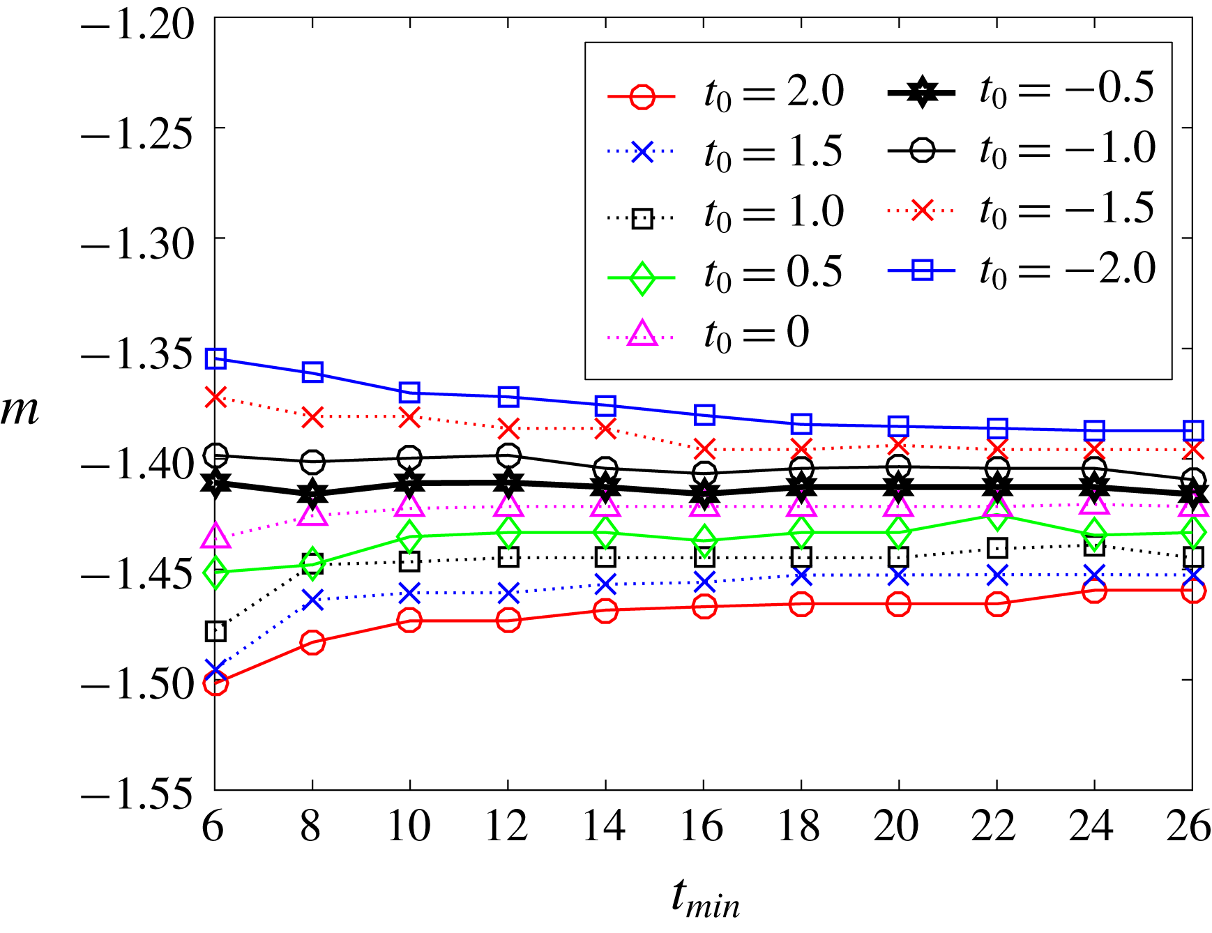
. Figure 5 shows the variation of
 $m$
with
 $t_{min}$
for different values of
 $t_{0}$
for
 $q_{u_{2}^{\prime }}^{2}$
. The uncertainties on the power-law parameters are
 $\unicode[STIX]{x0394}t_{0}\pm 0.5$
and
 $\unicode[STIX]{x0394}m\pm 0.01$
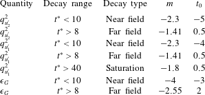
and table 5 shows the results of the power-law fitting process. Fits are made to the near field (
 $t^{\ast }<10$
) and far field (
 $t^{\ast }>8$
) with a region of overlap of approximately two eddy turnover times. An additional fit is made for the decay on the saturation regime;
 $t^{\ast }>40$
for
 $q_{u_{1}^{\prime }}^{2}$
. We also evaluate the uncertainty of the decay coefficients due to the statistical convergence of the
 $75$
runs. We investigate the decay coefficient of ensemble averages of
 $45$
and
 $60$
randomly picked cases using a pseudo-random algorithm implemented in Matlab. We find that the deviation of the decay coefficient
 $m$
for the ensemble averages of
 $45$
cases is within
 $5\,\%$
of the complete set and it reduces to
 $3\,\%$
for ensemble averages of
 $60$
cases. Thus, we propose to use the deviation in the ensemble average of
 $60$
cases as the maximum uncertainty in the determination of
 $m$
for the
 $75$
cases.
Variations of the exponent of the decay
 $m$
with various
 $t_{min}$
for a set of virtual origins
 $t_{0}$
. These results correspond to the far-field data for
 $q_{u_{2}^{\prime }}^{2}$
. The black thick line indicates the algorithm’s chosen solution.

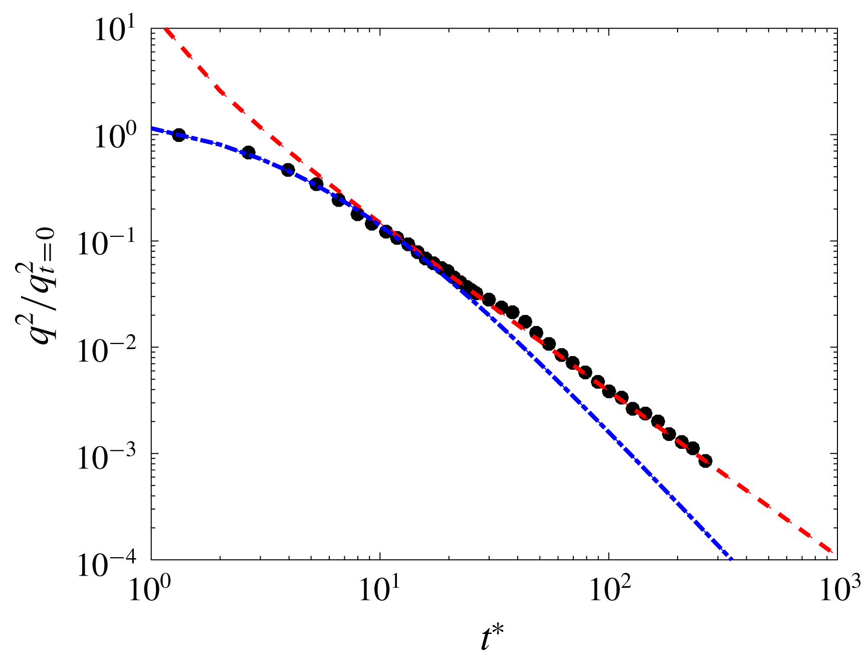
Time evolution of non-dimensional turbulent kinetic energy during the decay;
 $q^{2}/q_{t=0}^{2}$
. The dashed-dotted line represents the near field and the dashed line the far field. Details about the fitting procedure are in included in this section and the fitted parameters are shown in table 4.

Fitted constants for the power-law decay of
 $q^{2}$
. Near-field and far-field fits are made for data at
 $t^{\ast }<10$
and
 $t^{\ast }>8$
, respectively.

First, we investigate the decay of
 $q^{2}$
under the assumption of axisymmetric turbulence;
 $q^{2}=u_{1}^{\prime 2}+2u_{2}^{\prime 2}$
. In figure 6 one can see that the near- and far-field fits clearly differ. The decay exponent found for the near field (
 $m\approx -2.3$
) is similar to the values obtained in fractal-element grids for regions close to the grid where turbulence has not fully developed;
 $m\approx -2.5$
in Valente & Vassilicos (Reference Valente and Vassilicos2011) or
 $m\approx -2.8$
in Hearst & Lavoie (Reference Hearst and Lavoie2014) among others. In contrast, the far-field decay shows a decay exponent (
 $m=-1.55$
) slightly higher that previous wind tunnel experiments (
 $m\approx -1.39$
in Hearst & Lavoie (Reference Hearst and Lavoie2014) or
 $m=[-1.15,-1.25]$
in Valente & Vassilicos (Reference Valente and Vassilicos2012)) and DNS studies (
 $m=[-1.19,-1.39]$
in Burattini et al. (Reference Burattini, Lavoie, Agrawal, Djenidi and Antonia2006)).
We hypothesize that the value of the decay exponent might be affected by the confinement of turbulence. Therefore, to investigate this phenomenon we compare the evolution of each velocity component separately, i.e.
 $q_{u_{1}^{\prime }}^{2}=u_{1}^{\prime 2}$
and
 $q_{u_{2}^{\prime }}^{2}=u_{2}^{\prime 2}$
. These magnitudes are made non-dimensional with
 $q_{t=0}^{2}$
.
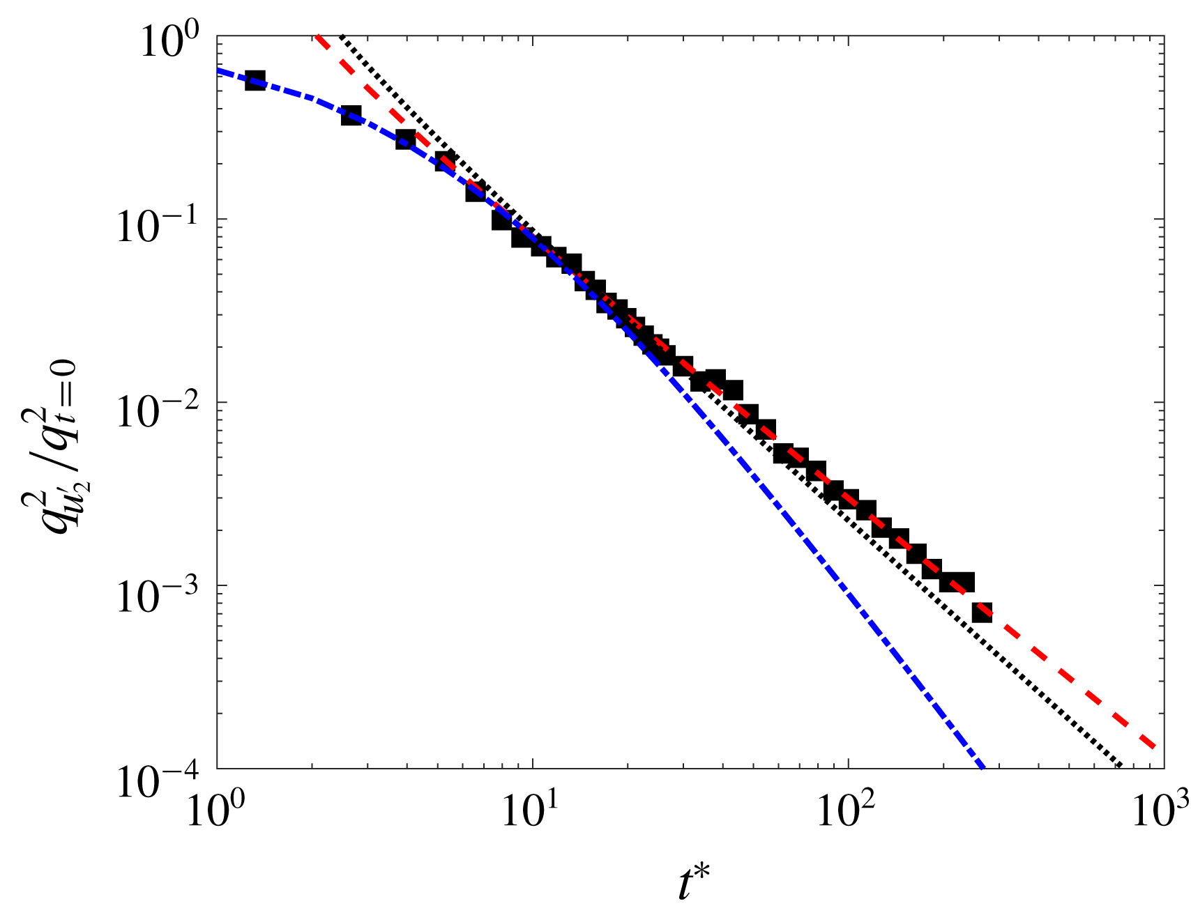
Time evolution of the non-dimensional turbulent kinetic energy from vertical velocity fluctuations (
 $q_{u_{2}^{\prime }}^{2}/q_{t=0}^{2}$
) during the natural decay. The dashed-dotted line represents the near field, the dashed line the far field and the dotted line the far-field fit of
 $q^{2}$
for comparison. Fitted parameters are shown in table 5.

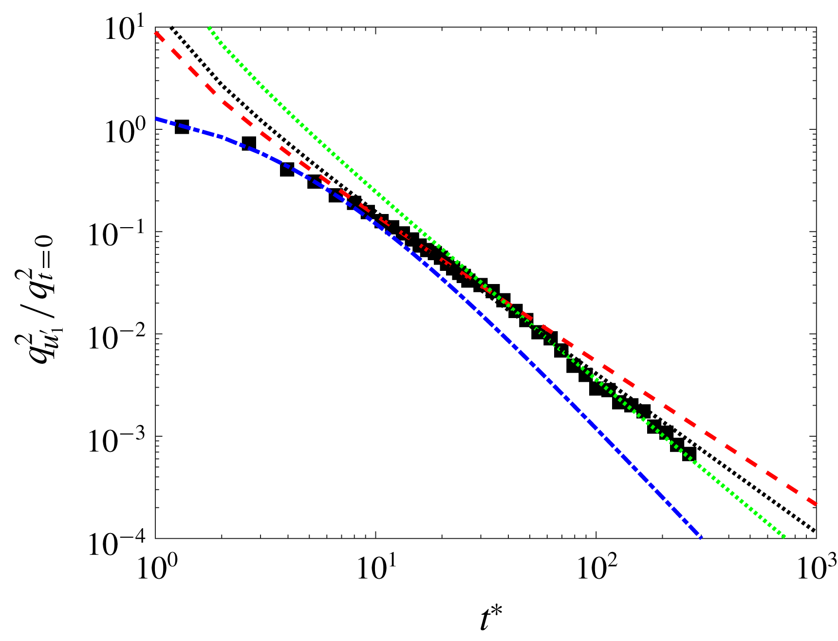
Time evolution of the non-dimensional turbulent kinetic energy from horizontal velocity fluctuations (
 $q_{u_{1}^{\prime }}^{2}/q_{t=0}^{2}$
) during the natural decay. The dashed-dotted line represents the near field, the dashed line the ‘first’ far field, the green dotted line the ‘saturated’ far field and the black dotted line the far-field fit of
 $q^{2}$
for comparison. Fitted parameters are shown in table 5.

Time evolution of the turbulent quantities during the natural decay;
 $q_{u_{1}^{\prime }}^{2}/q_{t=0}^{2}$
and
 $q_{u_{2}^{\prime }}^{2}/q_{t=0}^{2}$
(a), Taylor length scales (
 $\unicode[STIX]{x1D706}_{i}$
) (b) and integral length scales (
 $L_{ii}$
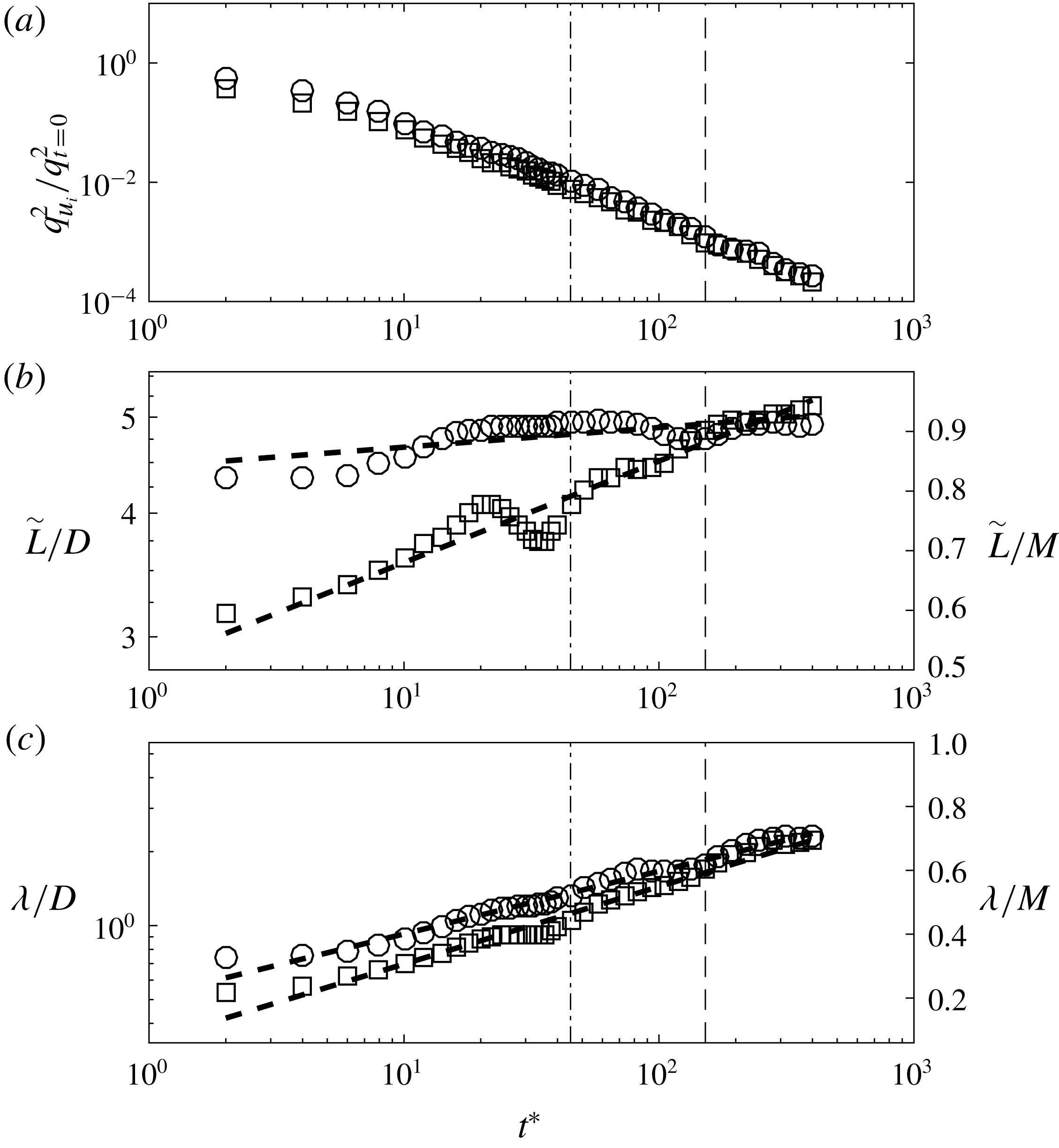
) (c). Circles and squares correspond to experimental data obtained from horizontal and vertical velocity fluctuations respectively. The dashed-dotted line represents the start of the saturation effects for the horizontal velocity fluctuations and the broken line the start of the large-scale isotropy regime.

Figure 7 shows that both the near field and far field of the
 $q_{u_{2}^{\prime }}^{2}$
decay can be well captured using their corresponding virtual origins and decay rates. We believe the near-field region is dominated by the turbulence production mechanism and therefore might be strongly facility dependent. The decay exponent found for the near field (
 $m\approx -2.3$
) is consistent with the result from
 $q^{2}$
presented before. In contrast, the decay exponent found in the far-field regime (
 $m\approx -1.4$
) is closer to the results previously exposed from wind tunnel experiments. This result also agrees with numerical calculation studies for which values of
 $m\approx -1.4$
have been obtained for Batchelor turbulence (Meldi & Sagaut Reference Meldi and Sagaut2017).
In figure 8, the evolution of
 $q_{u_{1}^{\prime }}^{2}$
shows a near-field decay as in
 $q_{u_{2}^{\prime }}^{2}$
. However, the far-field decay shows two different decay trends; far field without saturation (
 $t^{\ast }<40$
) and far field with saturation (
 $t^{\ast }>40$
). We find that when saturation is not present (
 $t^{\ast }<40$
), the decay rate is
 $m=-1.41$
and this is consistent with the result found for
 $q_{u_{2}^{\prime }}^{2}$
. However, the decay rate increases in the
 $t^{\ast }>40$
region due to saturation, leading to an exponent of
 $m=-1.8$
. The enhancement of the decay rate due to saturation effects is therefore the reason why the overall decay rate of
 $q^{2}$
shown in table 4 is higher than what it would be expected for natural decaying turbulence. We hypothesize that the final period of the decay is dominated by turbulence saturation and this will be further discussed in the current section. In fact, the magnitude of the decay rate is very close to the results obtained in Hwang & Eaton (Reference Hwang and Eaton2004) for the decay of isotropic turbulence in a confined domain. Also, Meldi & Sagaut (Reference Meldi and Sagaut2017) studied the sensitivity of the decay exponent to saturation effects and showed that, for a intermediate configuration between the fully unbounded case and the completely saturated case, the decay exponent increased to
 $m\approx -1.7$
, being in good agreement with the results found herein.
The aforementioned large-scale anisotropy can be clearly observed when both components are compared, as in figure 9(a). In fact,
 $q_{u_{1}^{\prime }}^{2}$
appears to be approximately 60 % stronger than the vertical counterpart (
 $q_{u_{2}^{\prime }}^{2}$
) for forced turbulence and small values of
 $t^{\ast }$
. However, this difference becomes less prominent as turbulence decays, and after
 $t^{\ast }\approx 150$
both quantities collapse into a single curve, as observed in figure 9(a).
As turbulence decays in time, the integral length scale grows in size and therefore the extrapolated region in the correlation function obtained from the PIV data also does so. We find that the results of the integral length scale are very sensitive to the shape of the last region of the correlation function. To overcome this issue we propose to look at a magnitude proportional to the integral length scale (
 $\tilde{L_{ii}}$
), that is the direct measure of the area under the correlation function without accounting for the region that should be extrapolated to obtain the true magnitude. We integrate the area under the correlation function for a square region of
 $4400~\text{px}$
to account for the original rectangular shape of the image sensor. In figure 9(b) we observe that
 $\tilde{L_{ii}}$
of the velocity fluctuations in the vertical direction grows logarithmically during all of the decay region recorded. In contrast, its horizontal counterpart grows rapidly during the initial period of the decay and then reaches a plateau at approximately
 $t^{\ast }=40$
. This plateau corresponds to the approximate critical time when
 $q_{u_{1}^{\prime }}^{2}$
experiences a faster decay over time, as seen in figure 9(a). Therefore, we believe that the sudden change in the decay rate of
 $q_{u_{1}^{\prime }}^{2}$
is dominated by turbulence saturation. This would also explain why the vertical counterpart
 $q_{u_{2}^{\prime }}^{2}$
, characterized by a smaller integral length scale, maintains the same decay rate during the experiments.
On the other hand, the evolution of the Taylor length scale (
 $\unicode[STIX]{x1D706}$
) is found to grow logarithmically in time along both directions;
 $x_{1}$
and
 $x_{2}$
, as shown in figure 9(c). However, the rate of growth differs from one to another and at large decay times both quantities have a similar length. This trend suggests that while turbulence saturation restricts the growth of large scales, small scales keep growing in time and therefore the inertial range
 $L(t)/\unicode[STIX]{x1D702}(t)$
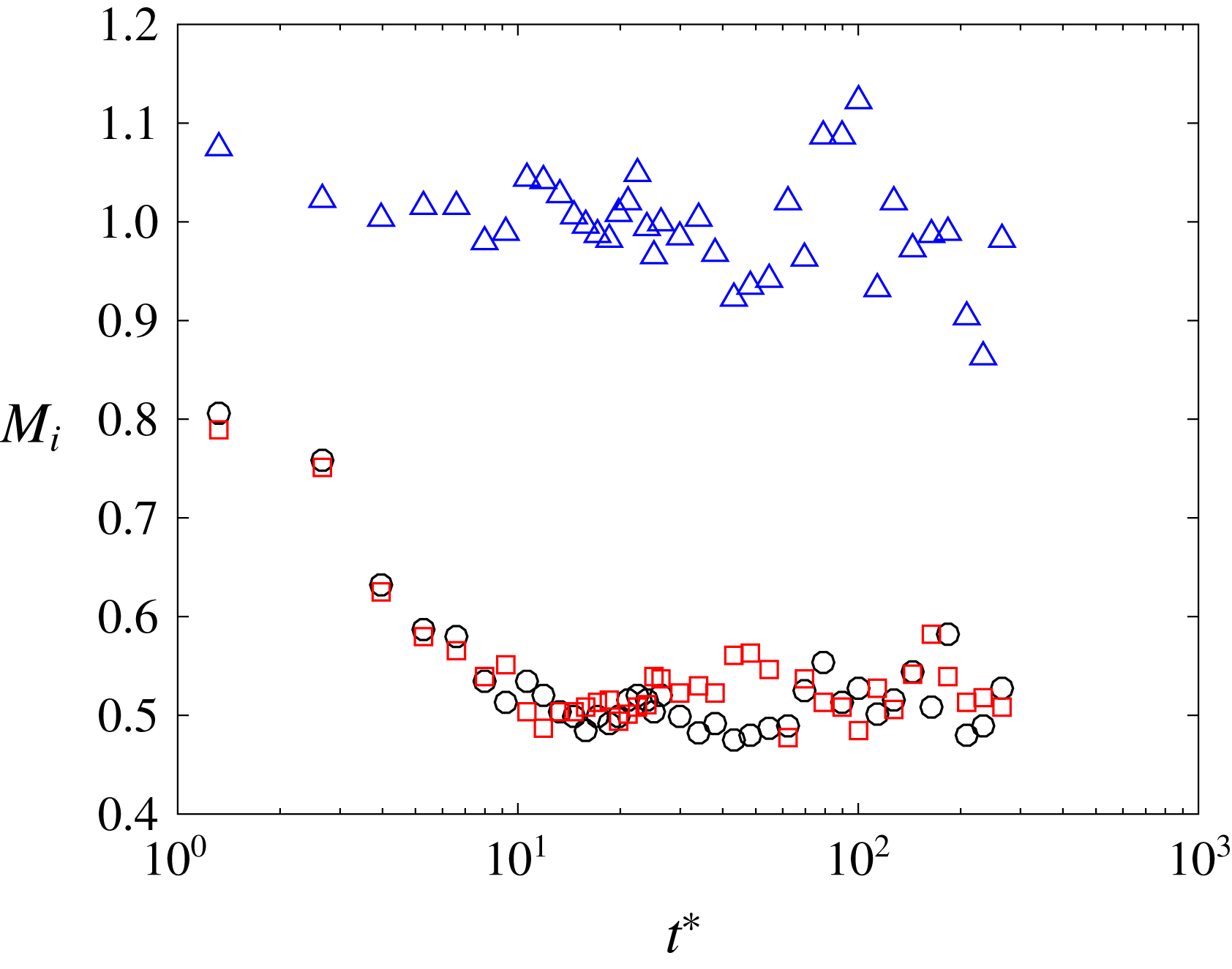
shrinks monotonically during the decay, as discussed in Biferale et al. (Reference Biferale, Boffetta, Celani, Lanotte, Toschi and Vergassola2003). To evaluate the evolution of the small-scale anisotropy during the decay we also compute the longitudinal and transverse velocity gradients, as in § 3. The small-scale anisotropy is then evaluated by computing the following ratios;
 $M_{1}=\langle (\unicode[STIX]{x2202}u_{1}/\unicode[STIX]{x2202}x_{1})/(\unicode[STIX]{x2202}u_{2}/\unicode[STIX]{x2202}x_{2})\rangle$
,
 $M_{2}=\langle (\unicode[STIX]{x2202}u_{1}/\unicode[STIX]{x2202}x_{1})/(\unicode[STIX]{x2202}u_{1}/\unicode[STIX]{x2202}x_{2})\rangle$
and
 $M_{3}=\langle (\unicode[STIX]{x2202}u_{2}/\unicode[STIX]{x2202}x_{2})/(\unicode[STIX]{x2202}u_{2}/\unicode[STIX]{x2202}x_{1})\rangle$
, and these are shown in figure 10. We observe that the longitudinal velocity ratio (
 $M_{1}$
) fluctuates about unity whereas the longitudinal to transverse ratios (
 $M_{2}$
,
 $M_{3}$
) quickly approach the relation
 $2\langle \unicode[STIX]{x2202}u_{i}/\unicode[STIX]{x2202}x_{i}\rangle \approx \langle \unicode[STIX]{x2202}u_{i}/\unicode[STIX]{x2202}u_{j}\rangle$
as one would expect for homogeneous isotropic turbulence. Further assessment of the turbulence natural decay can be made by estimating the skewness
 $S_{u_{i}}$
, where
 $$\begin{eqnarray}S_{u_{i}}\equiv \frac{\overline{\left(\displaystyle \frac{\unicode[STIX]{x2202}u_{i}}{\unicode[STIX]{x2202}x_{i}}\right)^{3}}}{\left[\overline{\left(\displaystyle \frac{\unicode[STIX]{x2202}u_{i}}{\unicode[STIX]{x2202}x_{i}}\right)^{2}}\right]^{3/2}}.\end{eqnarray}$$
For the case of HIT, the velocity skewness corresponds to the rate of production of vorticity through vortex stretching, as shown in Taylor (Reference Taylor1938). Due to its significance, predictions of
 $S$
as a function of the turbulence Reynolds number
 $Re_{\unicode[STIX]{x1D706}}$
have been extensively investigated in the past, see Sreenivasan & Antonia (Reference Sreenivasan and Antonia1997), and the recent work of Burattini, Lavoie & Antonia (Reference Burattini, Lavoie and Antonia2008) and Antonia et al. (Reference Antonia, Tang, Djenidi and Danaila2015) among others.
Time evolution of the ratio of velocity gradients during the natural decay. The triangles, circles, squares represent the gradient velocity ratios
 $M_{1}=\langle (\unicode[STIX]{x2202}u_{1}/\unicode[STIX]{x2202}x_{1})/(\unicode[STIX]{x2202}u_{2}/\unicode[STIX]{x2202}x_{2})\rangle$
,
 $M_{2}=\langle (\unicode[STIX]{x2202}u_{1}/\unicode[STIX]{x2202}x_{1})/(\unicode[STIX]{x2202}u_{1}/\unicode[STIX]{x2202}x_{2})\rangle$
and
 $M_{3}=\langle (\unicode[STIX]{x2202}u_{2}/\unicode[STIX]{x2202}x_{2})/(\unicode[STIX]{x2202}u_{2}/\unicode[STIX]{x2202}x_{1})\rangle$
, respectively.

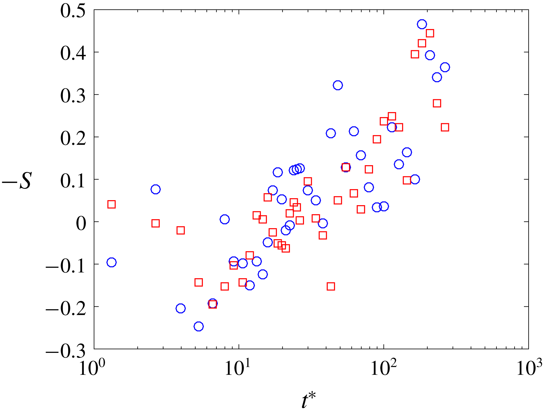
Skewness evolution during the decay. Circles and squares represent the horizontal and vertical statistics respectively (
 $-S_{u_{1}}$
and
 $-S_{u_{2}}$
).

Figure 11 shows that
 $-S_{u_{1}}$
and
 $-S_{u_{2}}$
are near zero at the start of the decay when turbulence might be affected by the forcing scheme, but these quantities increase during the decay to reach a value of
 $-S\approx 0.5$
. This value is in good agreement with the experimental and numerical results on the literature (
 $-S\approx 0.53$
in Antonia et al. (Reference Antonia, Tang, Djenidi and Danaila2015)). However, the skewness evolution appears to be very fluctuating during the decay and we believe that this effect might come from the increase in size of the turbulent structures, leading to fewer independent eddies per velocity field recorded causing a lack of statistical convergence. Also, the uncertainty in the velocity derivative skewness from PIV noise might be influencing the spread of this parameter.
Similarly, the evolution in time of the TKE dissipation rate is also investigated. We estimate it as detailed in § 3. However, as time elapses and turbulence decays, the turbulent scales of the flow grow in time and therefore the size of the Gaussian filter (
 $3\unicode[STIX]{x1D702}$
) becomes time dependent. To find the appropriate filter size we follow an iterative process for each data set in time that is as follows: First we filter the PIV velocity field with a Gaussian filter corresponding to
 $3\unicode[STIX]{x1D702}$
(estimated from the ‘stationary’ forced turbulence), we use the filtered velocity field to estimate the TKE dissipation rate and make a first estimation of the Kolmogorov length scale
 $\unicode[STIX]{x1D702}_{t}$
. This value of
 $\unicode[STIX]{x1D702}_{t}$
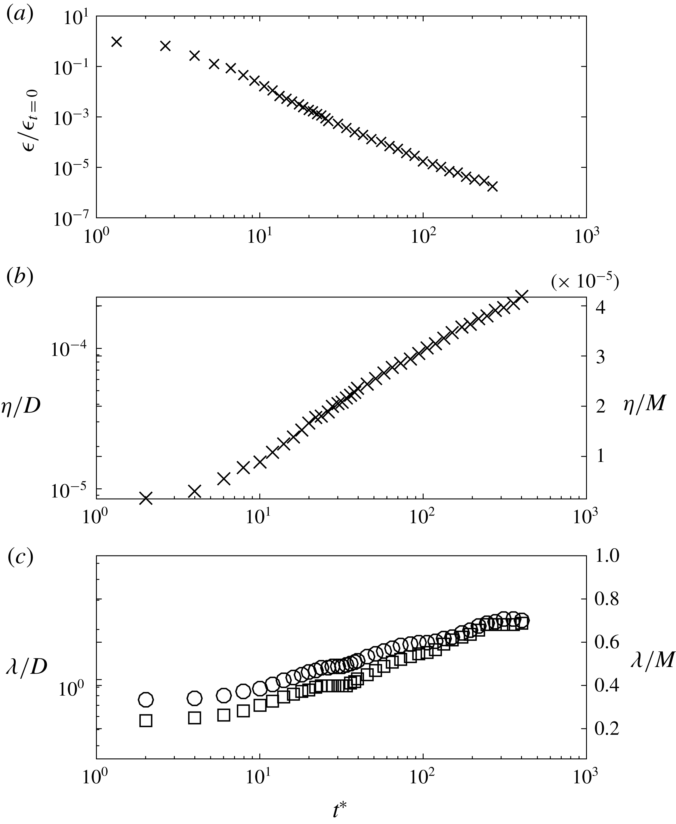
is used to filter again the original PIV velocity field and to make a second estimation of the TKE dissipation rate and Kolmogorov length scale. This process is repeated until the estimation of the TKE dissipation rate obtained from the filtered data is within 1 % of the previous iteration. The results obtained from this method are shown in figure 12(a).
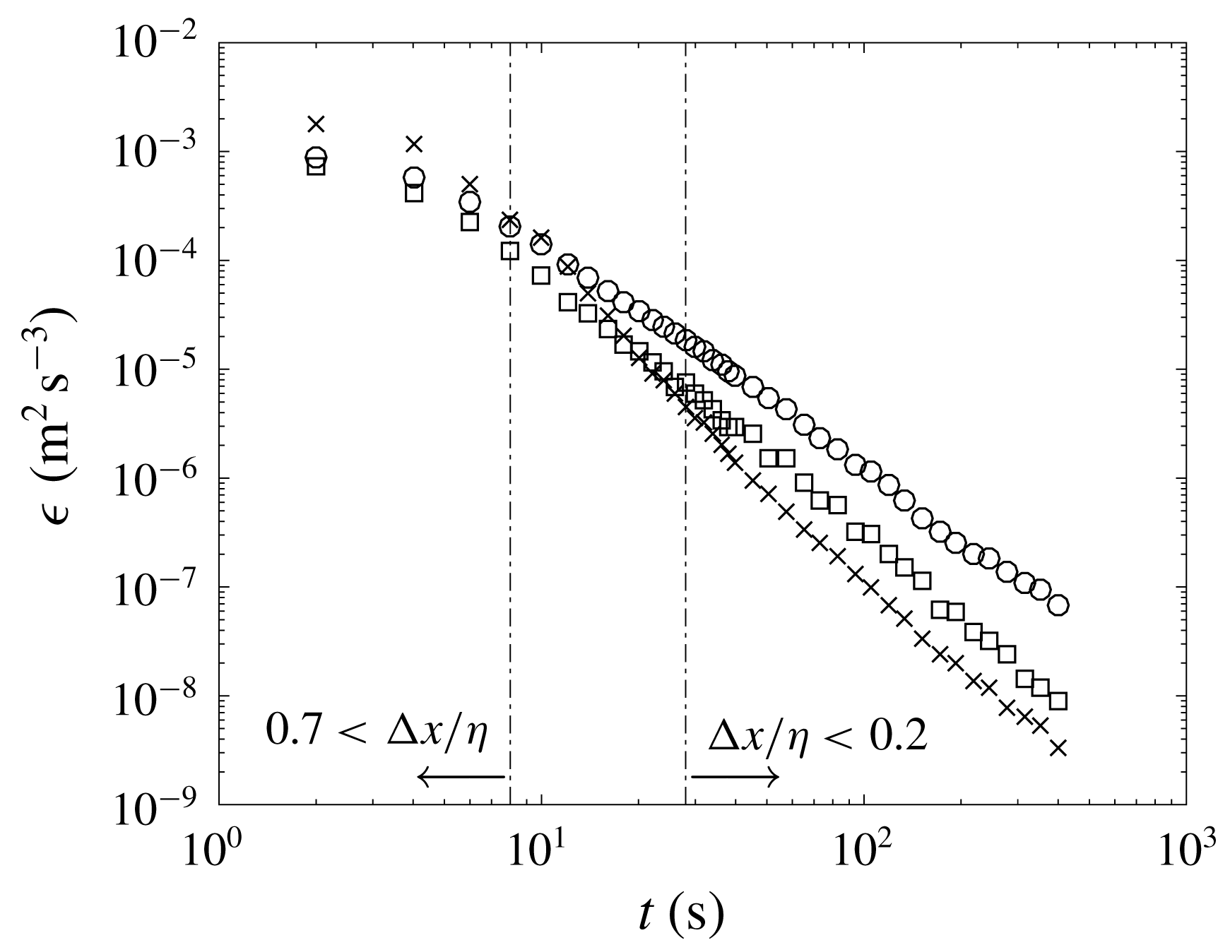
In addition to this direct method, we also compute the TKE dissipation rate using the method introduced by Tanaka & Eaton (Reference Tanaka and Eaton2007) for sub-Kolmogorov resolution, detailed in appendix A. This method was reported to give accurate results for a range of vector spacing (
 $\unicode[STIX]{x0394}x$
) to Kolmogorov length scale (
 $\unicode[STIX]{x1D702}$
) ratios of
 $0.7>\unicode[STIX]{x0394}x/\unicode[STIX]{x1D702}>0.2$
. According to our estimates, this range only includes a small region of the decay, detailed in figure 16 (appendix A). The results obtained from the method proposed by Tanaka & Eaton (Reference Tanaka and Eaton2007) appear to underestimate dissipation for
 $\unicode[STIX]{x0394}x/\unicode[STIX]{x1D702}>0.5$
and start to overestimate dissipation for
 $0.2<\unicode[STIX]{x0394}x/\unicode[STIX]{x1D702}$
. This agrees well with the results obtained from the iterative filtered data and gives us confidence in the iterative filtering method. The results from this method are now used to calculate the evolution of the Kolmogorov length scale over time. As observed for the Taylor length scale, the evolution of the Kolmogorov length scale appears to be unaffected by the saturation of the large scales, as shown in figure 12(b).
Time evolution of TKE dissipation rate (
 $\unicode[STIX]{x1D716}$
), Kolmogorov length scale (
 $\unicode[STIX]{x1D702}$
) and Taylor length scale (
 $\unicode[STIX]{x1D706}$
) during the natural decay.
 $M$
stands for the centre-to-centre nozzle distance and
 $D$
for the nozzle internal diameter.

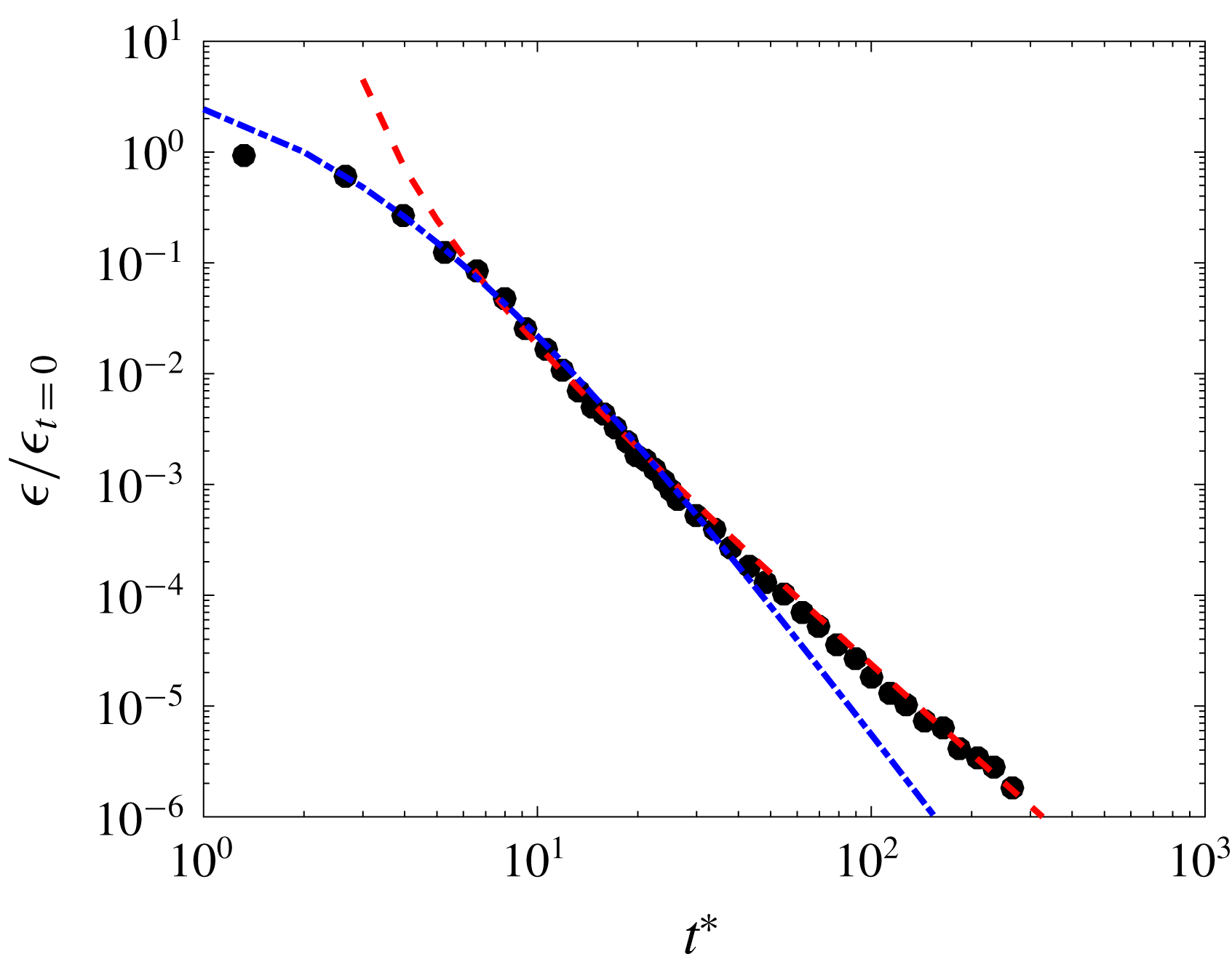
Also, the results of the TKE dissipation rate from the iterative filtering method are fitted to a power-law equation in figure 13, following the same technique as for
 $q^{2}$
. Again, the evolution of the TKE dissipation rate over time can be divided in two regimes. The near-field regime can be fitted to a power-law function with
 $m=-4$
and
 $t_{0}=-3$
, whereas the fit for the far-field regime gives
 $m=-2.55$
and
 $t_{0}=2$
. This result agrees well with the relation obtained from the energy budget for isotropic homogeneous turbulence naturally decaying in absence of production terms; i.e.
 $m_{\unicode[STIX]{x1D716}}=m-1$
, and gives us confidence in the accuracy on the method used.
Time evolution of TKE dissipation rate estimate (
 $\unicode[STIX]{x1D716}_{G}$
) during the natural decay. The dashed-dotted line represents the near field and the dashed line the far field. Fitted parameters are shown in table 5.

Fitted constants for the power-law decay of turbulent quantities. Near-field and far-field fits are made for data at
 $t^{\ast }<10$
and
 $t^{\ast }>8$
respectively.

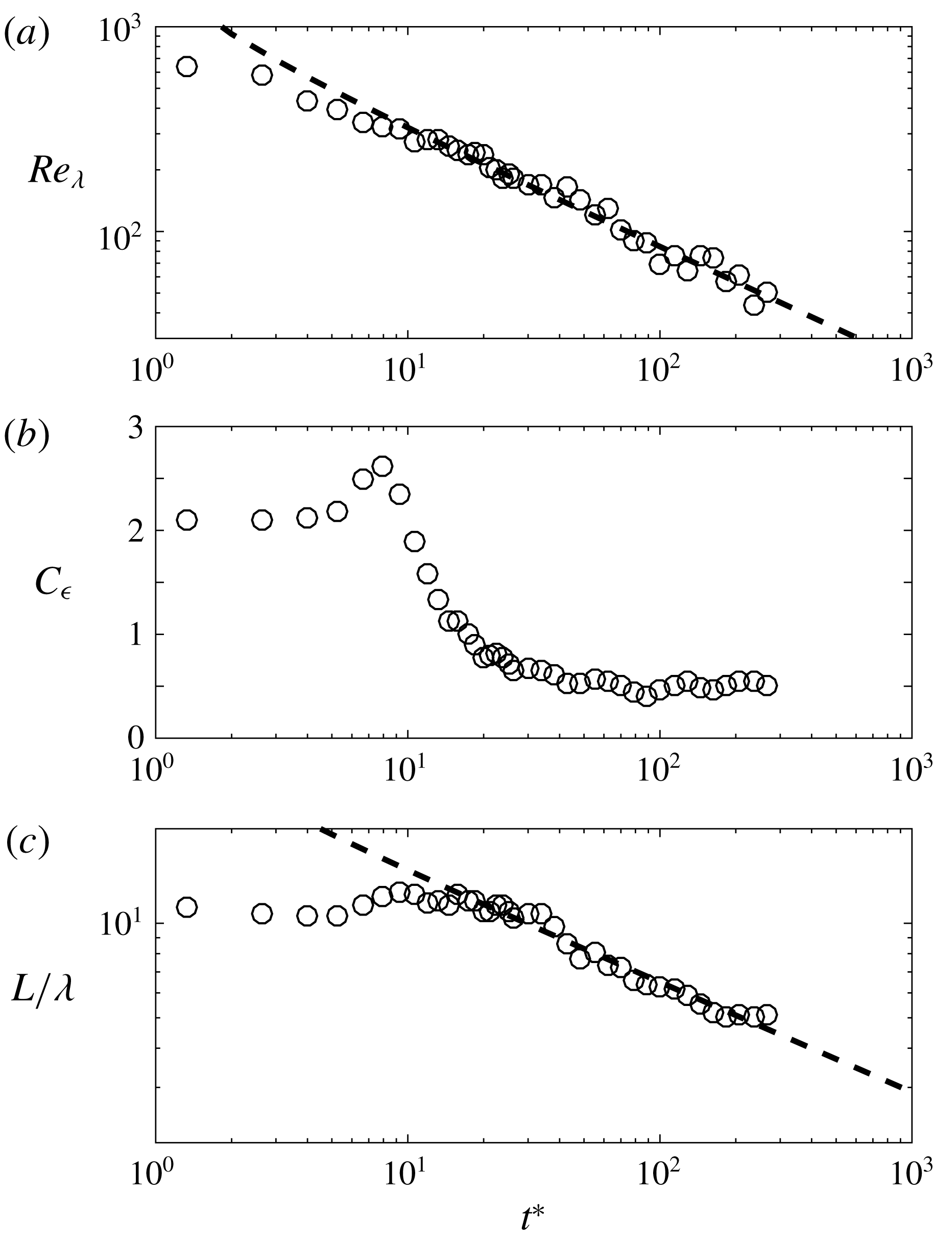
Finally, in figure 14, we investigate the evolution of the Reynolds number based on the Taylor length scale (
 $Re_{\unicode[STIX]{x1D706}}$
), the value of
 $C_{\unicode[STIX]{x1D716}}$
and the evolution of the integral length scale to Taylor length scale (
 $L/\unicode[STIX]{x1D706}$
) during the decay. We observe the Reynolds number (
 $Re_{\unicode[STIX]{x1D706}}$
) for
 $t^{\ast }=0$
to be slightly higher than the value obtained for ‘stationary’ turbulence. However, this might be due to the finite number of runs computed (
 $75$
for the decay) and not a physical phenomenon, as occurs in regions very close to the turbulence-generating grid in wind tunnel experiments, as reviewed in Vassilicos (Reference Vassilicos2015). Then, as turbulence decays the Reynolds number decreases logarithmically with time. The decay exponent of the Reynolds number (
 $m_{Re_{\unicode[STIX]{x1D706}}}\approx -0.57$
) agrees very well with previously reported values in Compte-Bellot & Corrsin (Reference Compte-Bellot and Corrsin1966) and revisited by Meldi & Sagaut (Reference Meldi and Sagaut2014), where
 $m_{Re_{\unicode[STIX]{x1D706}}}=-0.5$
for complete saturation. The value of
 $C_{\unicode[STIX]{x1D716}}$
during the first stage of the decay is unusual if compared with most of decaying grid-generated turbulence (Valente & Vassilicos Reference Valente and Vassilicos2012; Hearst & Lavoie Reference Hearst and Lavoie2014). However, the trend in the evolution of
 $C_{\unicode[STIX]{x1D716}}$
agrees very well with the results from grid-generated turbulence in Djenidi et al. (Reference Djenidi, Lefeuvre, Kamruzzaman and Antonia2017), where the authors showed a decaying value of
 $C_{\unicode[STIX]{x1D716}}$
for the near-field decay region. This suggests that the near-field decay of the turbulence generated does not comply with the self-preservation requirement that would, in turn, return a constant value for
 $C_{\unicode[STIX]{x1D716}}$
. However,
 $C_{\unicode[STIX]{x1D716}}$
becomes stable once the turbulence has fully developed and the influence of the forcing mechanism becomes negligible. It is also interesting to note that
 $C_{\unicode[STIX]{x1D716}}$
remains nearly constant for
 $200>Re_{\unicode[STIX]{x1D706}}>20$
where the flow suffers from confinements effects. On the other hand, the ratio
 $L/\unicode[STIX]{x1D706}$
fluctuates about a value of
 ${\approx}12$
for the near-field decay, but for
 $t^{\ast }>40$
it decreases logarithmically in time with a decay exponent
 $m_{L/\unicode[STIX]{x1D706}}\approx -0.35$
. Again, the decay region in the
 $L/\unicode[STIX]{x1D706}$
ratio corresponds to the saturated regime, where large scales are constrained by the facility but small and intermediate scales are still growing.
Time evolution of the Reynolds number based on the Taylor length scale (
 $Re_{\unicode[STIX]{x1D706}}$
) (a), of
 $C_{\unicode[STIX]{x1D716}}=\unicode[STIX]{x1D716}L_{11}/u^{\prime 3}$
(b) and the integral length scale to Taylor length scale (
 $L/\unicode[STIX]{x1D706}$
) (c) during the natural decay.

5 Conclusion
We investigated the evolution of anisotropic turbulence at large scales during natural decay in an experiment with initial Reynolds number (based on the Taylor microscale
 $\unicode[STIX]{x1D706}$
)
 $Re_{\unicode[STIX]{x1D706}}\approx 580$
over more than two decades in time. In contrast with wind tunnel experiments where Taylor’s hypothesis is invoked to convert downstream distance
 $x$
(generally made dimensionless as
 $x/L_{0}$
) into time, we directly observe the evolution of turbulence over time and use the eddy turnover time (
 $t_{L}$
) of the ‘stationary’ forced turbulence to make the time evolution dimensionless (
 $t/t_{L}$
). As turbulence decays and the large scales of the flow start to grow in size, these become large enough to feel the boundaries of the facility that contains them, leading to turbulence saturation. Then, the sensitivity of free decaying anisotropic turbulence to saturation effect was investigated.
Ninety-six water-pump-driven jets pointed towards the centre of the rectangular water tank from opposite sides and were driven randomly following the ‘Sunbathing algorithm’ introduced in Variano & Cowen (Reference Variano and Cowen2008) to produce anisotropic turbulence, instead of the HIT obtained in previous studies with a similar facility (Bellani & Variano Reference Bellani and Variano2013). This forcing scheme for the facility presented produced a central volume of turbulence that had negligible shear, mean flow and was homogeneous. When the tank is in operation we observe a turbulent flow for which the ratio of horizontal to vertical velocity fluctuations is
 $u_{1}^{\prime }/u_{2}^{\prime }\approx 1.22$
, with a ratio of integral length scales of
 $L_{11}/L_{22}\approx 1.6$
.
The two RJAs were turned off after
 $5$
minutes of active forcing and
 $40$
pairs of images were acquired with variable
 $dt$
to limit the particle pixel displacement to
 $4{-}6~\text{px}$
. and reduce out-of-plane motion. This process was repeated
 $75$
times and results were ensemble averaged.
The natural decay of the flow was investigated for individual components of the velocity fluctuation. We observed that the large-scale anisotropy that exists at the start of the decay is progressively reduced and becomes statistically negligible for
 $t^{\ast }>150$
. We believe this process have been enhanced by the saturation effect over the large scales of the flow, since the integral scales in the horizontal direction started to be affected by the boundaries of the facility much sooner than their vertical counterpart, driving the fast return to isotropy. Power-law fits were obtained for
 $q^{2}$
,
 $q_{u_{1}^{\prime }}^{2}$
and
 $q_{u_{2}^{\prime }}^{2}$
and
 $\unicode[STIX]{x1D716}$
following the method proposed in Hearst & Lavoie (Reference Hearst and Lavoie2014). We observed a very similar behaviour of
 $q_{u_{1}^{\prime }}^{2}$
and
 $q_{u_{2}^{\prime }}^{2}$
over time as compared with wind tunnel experiments equipped with multi-fractal passive and active grids (Krogstad & Davidson Reference Krogstad and Davidson2011; Valente & Vassilicos Reference Valente and Vassilicos2011, Reference Valente and Vassilicos2012; Hearst & Lavoie Reference Hearst and Lavoie2014); and numerical simulations (Meldi, Sagaut & Lucor Reference Meldi, Sagaut and Lucor2011; Perot Reference Perot2011) for Batchelor turbulence. Two different regimes are observed for free decaying turbulence. First, we observe a fast decay of the TKE for
 $t^{\ast }<10$
. This region is present in wind tunnel experiments for a few integral length scales downstream of the grid and is referred to as ‘near-field’ decay. This regime is believed to be strongly affected by the turbulence production mechanism as discussed in Meldi (Reference Meldi2016) and therefore to be ‘facility dependent’. Then, we observe a second region of logarithmically decaying TKE for
 $t^{\ast }>8$
. This region is also present in wind tunnel experiments after a distance of about
 $20L_{11}$
downstream of the grid and is referred to as ‘far-field’ decay. The decay exponent of this region, either in time in numerical studies or in space in wind tunnel experiments, has been a matter of debate during the past several decades. Wind tunnel experiments have shown that this decay region is non-universal and that different turbulence generators lead to changes in the decay rate. Here, we found the exponent of this region for the unsaturated case to be
 $m\approx 1.41$
and this is within the range of values observed for the ‘far-field’ decay in wind tunnel experiments and numerical results. Besides these two regimes, we found the turbulent kinetic energy to decay faster once large scales ‘feel’ the confinement effect, i.e. the integral length scale stops growing over time. The decay exponent during the saturation regime becomes
 $m\approx -1.8$
and therefore approaches the value obtained from analytical results for complete saturation in Skrbek & Stalp (Reference Skrbek and Stalp2000), that is
 $m=-2$
. The decay exponent of the saturation regime is also in good agreement with the decay exponent observed in Hwang & Eaton (Reference Hwang and Eaton2004) where, we believe, confinement effects were present. The anisotropy evolution of the small scales is investigated by comparing velocity gradients; i.e.
 $M_{1}$
,
 $M_{2}$
and
 $M_{3}$
. We found that after
 $t^{\ast }=10$
the relation between velocity gradients approaches the isotropic relation and this is consistent with the DNS study in Biferale et al. (Reference Biferale, Boffetta, Celani, Lanotte, Toschi and Vergassola2003) where they found small scales to ‘isotropize’ much quicker than large scales. Also, the dissipation rate of the TKE is estimated from direct measurements following an iterative filtering process. The goal of this process is to obtain the ‘true’ Kolmogorov length scale to filter the data using a Gaussian filter size of
 $3\unicode[STIX]{x1D702}$
as in Ganapathisubramani et al. (Reference Ganapathisubramani, Lakshminarasimhan and Clemens2007). The results from this estimate agree well with other direct and indirect methods, giving us confidence in the chosen approach. Also, the decay rate for the dissipation rate is found to be
 $m_{\unicode[STIX]{x1D716}}\approx -2.55$
and agrees well with the theoretical prediction of
 $m_{\unicode[STIX]{x1D716}}=m-1$
for free decaying turbulence.
Acknowledgements
This work was supported by Aquavitrum Ltd., the Engineering and Physical Sciences Research Council (1658462) and the Faculty of Engineering and Physical Sciences of University of Southampton. Pertinent data for this paper are available at doi:10.5258/SOTON/D0723.
Appendix A. Spatial gradients in PIV
A.1 Dissipation estimate from structure function
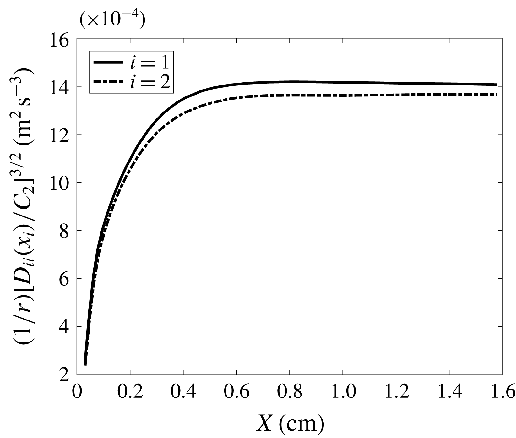
Second-order structure functions are defined as
 $$\begin{eqnarray}D_{ii}=\langle \overline{[u_{i}(x+r)-u_{i}(x)]^{2}}\rangle .\end{eqnarray}$$
For homogeneous isotropic turbulence and separation values
 $r_{i}$
within the inertial range and aligned with the velocity component
 $u_{i}$
, Kolmogorov’s theory states:
 $$\begin{eqnarray}D_{ii}(r_{i})=C_{2}(\unicode[STIX]{x1D716}r_{i})^{2/3},\end{eqnarray}$$
where
 $C_{2}=2.12$
as in Sreenivasan (Reference Sreenivasan1995). Thus, the compensated longitudinal second-order structure function in (A 2) can be used to find the magnitude of the TKE dissipation rate. This is obtained by looking at the plateau value reached in the inertial range.
Longitudinal structure functions for both unfiltered velocity components, compensated according to equation (A 2) to estimate TKE dissipation rate from the plateau value.

Time evolution of TKE dissipation rate during the natural decay. Squares represent values from compensated second-order structure function
 $D_{11}(r_{1})$
, circles the correction method of Tanaka & Eaton (Reference Tanaka and Eaton2007) and crosses show results after applying a Gaussian filter of size
 $3\unicode[STIX]{x1D702}$
as in proposed in Ganapathisubramani et al. (Reference Ganapathisubramani, Lakshminarasimhan and Clemens2007). The dashed-dotted lines show the working range of the method proposed in Tanaka & Eaton (Reference Tanaka and Eaton2007).

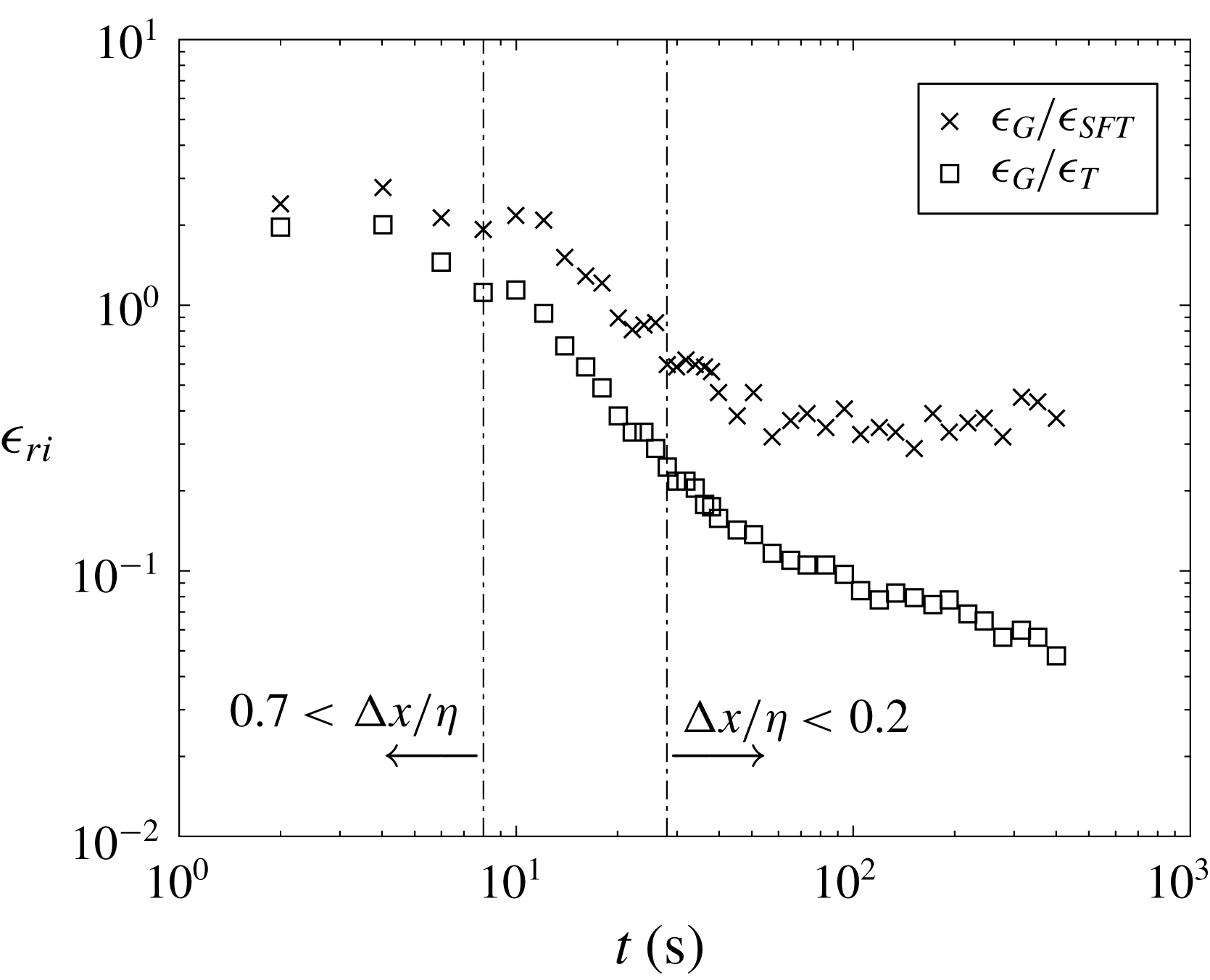
Time evolution of dissipation ratio
 $\unicode[STIX]{x1D716}_{ri}$
between the estimates of the TKE dissipation rate during the natural decay. The dashed-dotted lines show the working range of the method proposed in Tanaka & Eaton (Reference Tanaka and Eaton2007). The sub-indices
 $T$
and
 $G$
refer to the estimates based on the correction method proposed in Tanaka & Eaton (Reference Tanaka and Eaton2007) and the estimates based on a velocity Gaussian smoothing of
 $3\unicode[STIX]{x1D702}$
as in Ganapathisubramani et al. (Reference Ganapathisubramani, Lakshminarasimhan and Clemens2007).

A.2 Direct dissipation estimate from sub-Kolmogorov PIV resolution
This method was introduced in Tanaka & Eaton (Reference Tanaka and Eaton2007) as a direct method to estimate TKE dissipation rate from PIV data with sub-Kolmogorov resolution and it was formulated as
 $$\begin{eqnarray}\unicode[STIX]{x1D716}\cong \frac{4\unicode[STIX]{x1D716}_{D}|_{2\unicode[STIX]{x0394}x}-\unicode[STIX]{x1D716}_{D}|_{\unicode[STIX]{x0394}x}}{3},\end{eqnarray}$$
where the subscript
 $D$
denotes a quantity obtained from two-dimensional PIV data.
 $\unicode[STIX]{x1D716}_{D}|_{\unicode[STIX]{x0394}x}$
is the TKE dissipation rate using second-order central difference approximation and
 $\unicode[STIX]{x1D716}_{D}|_{2\unicode[STIX]{x0394}x}$
is the dissipation rate at double grid spacing.
According to our estimates this range only includes a small region of the decay (limited with dashed lines) in figure 16. For vector spacing ratios smaller than the working range, the TKE dissipation rate is underestimated, whereas for larger vector spacing ratios it is overestimated (Tanaka & Eaton Reference Tanaka and Eaton2007). This trend is consistent with the results presented here, as observed in figure 16. In figure 16 the two direct estimates of dissipation are plotted together with the indirect estimate (
 $D_{11}(r_{1})$
). Both longitudinal second-order compensated structure functions (
 $D_{11}(r_{1})$
,
 $D_{22}(r_{2})$
) give dissipation estimates that are within 30 % and therefore only
 $D_{11}(r_{1})$
is plotted for clarity. Despite the difference between the two direct methods for small decay times, this becomes less pronounced as turbulence decays and then the two methods maintain a very similar decay rate. In contrast, the estimate from the structure function agrees very well with the direct estimate from the data with a Gaussian spatial filter of
 $3\unicode[STIX]{x1D702}$
kernel size for the initial period of the decay, whereas the direct estimate from the correction method seems to underestimate dissipation. For longer decay times, the decay rate from the structure functions gets more pronounced and therefore closer to the estimate from the correction method. Both direct estimates of the TKE dissipation rate for the last section of the decay appear to overestimate the dissipation rate. This result is in agreement with Tanaka & Eaton (Reference Tanaka and Eaton2007), where they showed that their correction method underestimates dissipation for
 $\unicode[STIX]{x0394}x/\unicode[STIX]{x1D702}>0.5$
and starts to overestimate dissipation for
 $0.2<\unicode[STIX]{x0394}x/\unicode[STIX]{x1D702}$
. Figure 17 shows the time evolution of the dissipation ratios together with an estimate of the PIV spatial resolution in time as
 $\unicode[STIX]{x0394}x/\unicode[STIX]{x1D702}$
.