1. Introduction
The objective of the present research is to better understand two important processes in the near wake of a flat plate with a circular trailing edge and turbulent separating boundary layers, entrainment and instability of the detached shear layers (DSLs). Unlike the case of the cylinder, the Reynolds number based on momentum thickness of the boundary layer near separation (
 $\mathit{Re}_{{\bf\theta}}$
) and the Reynolds number defined using the thickness of the flat plate or the diameter of its trailing edge (
 $\mathit{Re}_{D}$
) are independent parameters. The data used here are obtained from direct numerical simulations (DNS) of flat-plate flow for different combinations of these two Reynolds numbers. The turbulent boundary layers and the wake are all computed via DNS. The separating boundary layers are statistically identical. Therefore, the wake is symmetric in the mean. The ratio
 ${\it\theta}/D$
in all these cases is sufficiently small, and this results in vigorous vortex shedding. Here, we continue the analysis of the near wake initiated in Rai (Reference Rai2010a
, Reference Rai2013, Reference Rai2014).
One of the earliest investigations of entrainment in a turbulent wake is by Townsend (Reference Townsend1966). It is observed there that entrainment is caused in part by small-scale vorticity diffusion and subsequent amplification by straining, a process that is referred to as ‘nibbling’. Townsend (Reference Townsend1966) also states that the folding of the bounding surface (the surface between the irrotational and turbulent regions) by large eddies (not necessarily shed vortices) can substantially increase the rate of entrainment. Here, entrainment refers to the ingestion of irrotational ambient fluid by the turbulent wake (or the advancement of turbulence in the wake into the irrotational ambient fluid). Many of the observations made in this article, such as the appearance, growth and eventual disappearance of indentations (due to large eddies) in the wake and the engulfing of ambient fluid by these regions of indentation, suggest that the primary concern of the author is the far wake. However, basic ideas such as nibbling by the small vortices and folding by the large ones should apply to the near wake as well. In contrast to the far wake, the near wake of bluff bodies such as cylinders is populated with shed vortices whose rotation contributes substantially to the engulfing of ambient fluid. Here, the term engulfing refers to the motion of ambient fluid into the region of the wake.
Bevilaqua & Lykoudis (Reference Bevilaqua and Lykoudis1971), based on experiments on the near wake of a sphere, observe that entrainment occurs in three phases: ambient fluid first deforms as the bounding interface approaches, it is then swirled into the wake by the spinning motion of large vortices associated with surface waves and turbulent mixing occurs in the final phase of entrainment. The rotation of the large vortices is the principal mechanism of wake growth. The authors do remark that the difference between Townsend’s ‘nibbling’ mechanism and their ‘entrainment by the rotation of large eddies’ may only be a matter of scale and that ‘the swirling action of the smallest eddies is probably similar to that of the largest’. Papailou & Lykoudis (Reference Papailou and Lykoudis1974) confirm the findings of Bevilaqua & Lykoudis (Reference Bevilaqua and Lykoudis1971), but in the context of the near wake of a cylinder. They observe that the turbulent vortex street is the origin of the convolutions on the wake surface and that these vortices draw ambient fluid into the wake because of their rotation. They also remark that a portion of this fluid remains within the vortices while the remainder diffuses into the turbulent core by the action of turbulence. Their flow visualization shows the shed vortices located on either side of a ‘core’ region that runs along the centreline of the wake. As will be seen later in this article, depending on the value of
 ${\it\theta}/D$
, a distinct core region may or may not exist in the wake. However, the braids connecting a given vortex to neighbouring vortices of opposite sign do exist. The authors also note that entrainment is strong in the near wake but weakens downstream where the vortices weaken and their ability to engulf ambient fluid decreases.
In more recent work, Cantwell & Coles (Reference Cantwell and Coles1983), based on cylinder wake data (near wake), observe that ambient fluid is induced to flow towards the wake centreline and even cross it between any two adjacent vortices, and that during this process the engulfed fluid is eventually entrained. They also observe that a shed vortex engulfs fluid from both sides of the wake, with a greater percentage of the fluid coming from the opposite side of the wake (except in the vortex formation region where it engulfs more fluid from the same side of the wake as it is located). A point of interest is that the entrainment velocity was found to vary over the boundary of a vortex; it was inferred that it was considerably larger on the upstream side of the vortex compared with the downstream side.
A considerable amount of research on entrainment in the far wake has appeared in the literature since Townsend’s (Reference Townsend1966) article. A fairly extensive survey of the findings can be found in Kopp, Giralt & Keffer (Reference Kopp, Giralt and Keffer2002). The role of turbulent bulges in entrainment, the coherent structures that comprise these bulges, the coherence of large-scale bulges as they travel downstream, the evolution of shed vortices into horse-shoe vortices, etc. are discussed in this paper. In contrast, the emphasis in the present paper is on entrainment in the near wake (less than
 $15D$
downstream of the trailing edge). In addition, the separating boundary layers are not laminar but turbulent, thus leading to a very different situation. While there is some similarity with the work of Papailou & Lykoudis (Reference Papailou and Lykoudis1974) and Cantwell & Coles (Reference Cantwell and Coles1983) in that rotational motion of the shed vortices is present, the fluid that is engulfed is not always irrotational ambient flow.
The first objective of the present study is to investigate the important features of the entrainment process in the context of the flat plate with turbulent separating boundary layers. As observed in Rai (Reference Rai2014), much of the log-layer region of the separating boundary layer does not participate in the vortex formation process but simply convects past the trailing edge. Hence, it is not irrotational ambient fluid that is engulfed by the shed vortices; instead we have the log layer and the ‘wake’ of the boundary layer being engulfed in the very near wake. Here, we provide (a) a visualization of the near-wake engulfment process including the assimilation of log-layer eddies etc., (b) a discussion of the effect of only a small portion of the boundary layer participating in the initial vortex roll-up process on near-wake velocity statistics and (c) results from a few different DNS to better understand the effect of
 ${\it\theta}/D$
on entrainment and near-wake physics in general.
Instability of the DSLs occurring in the wakes of cylinders has been studied extensively. Experimental, computational and theoretical means have been employed in these efforts. Roshko (Reference Roshko1953) first observed instability in the DSL. Measurements of fluctuating velocity near DSLs by Bloor (Reference Bloor1964) led to the discovery of ‘transition waves’ with frequency higher than the shedding frequency. These waves were found to result in a broadband peak in the velocity spectra obtained near the DSLs; the ratio of the shear-layer frequency (
 ${\it\omega}_{sl}$
, corresponding to the peak of the broadband region) and the shedding frequency (
 ${\it\omega}_{st}$
) was found to be proportional to the square root of
 $\mathit{Re}_{D}$
. Prasad & Williamson (Reference Prasad and Williamson1997) estimate the exponent to be approximately
 $2/3$
. Thompson & Hourigan (Reference Thompson and Hourigan2005) propose the use of different power-law fits for different ranges of
 $\mathit{Re}_{D}$
, with exponents closer to
 $1/2$
.
Unal & Rockwell (Reference Unal and Rockwell1988) demonstrated the exponential growth of the amplitude of velocity fluctuations in the shear layer with increasing streamwise distance (
 $x/D$
). They also detected the presence of two dominant frequencies in the corresponding spectra (
 ${\it\omega}_{sl}$
and
 ${\it\omega}_{st}$
), and peaks at
 ${\it\omega}_{sl}\pm {\it\omega}_{st}$
that they attributed to nonlinear interactions between fluctuations at the two frequencies. Prasad & Williamson (Reference Prasad and Williamson1997) explored intermittency in the shear-layer instability mechanism; the velocity fluctuations were observed to first increase in amplitude followed by a decrease. They classified intermittency events based on fluctuating amplitude (small and large in comparison to those at the shedding frequency) and proposed potential mechanisms that could result in the two observed levels of instability.
Computational investigations of the DSL instability in cylinder flows have also played an important role in obtaining a better understanding of this phenomenon in addition to the experimental studies mentioned above. Kim & Choi (Reference Kim and Choi2001) provide a large eddy simulation at
 $\mathit{Re}_{D}=3900$
. They propose two types of shear-layer instability: type A which is three-dimensional and is generated locally by a strong streamwise vortex pair underneath the DSL, and type B which is quasi-two-dimensional and is related to Karman vortex shedding. Dong et al. (Reference Dong, Karniadakis, Ekmekci and Rockwell2006) present a combined experimental/DNS study of cylinder wakes at
 $\mathit{Re}_{D}=3900$
and 10 000 with velocity spectra showing a peak at
 ${\it\omega}_{st}$
and also a broadband peak. Interestingly, at the higher Reynolds number, two peaks are observed in the broadband region. The average of the two corresponding frequencies agrees well with that predicted by the
 $2/3$
power law of Prasad & Williamson (Reference Prasad and Williamson1997).
A computation (DNS) of cylinder flow at
 $\mathit{Re}_{D}=3900$
was undertaken by Rai (Reference Rai2010a
) to investigate, among other things, the phenomenon of intermittency and the classification thereof by earlier investigators, the underlying causes of instability, the broadband nature of the corresponding peak in spectra and the three-dimensional structure of the instability events. An interaction between the shear layer and vortices in the recirculation region was determined to be a principal cause for both the initiation and growth of the instability. A classification of shear-layer instability events that is different from those of Prasad & Williamson (Reference Prasad and Williamson1997) and Kim & Choi (Reference Kim and Choi2001) is proposed in Rai (Reference Rai2010a
). A simple analysis, based on the inviscid incompressible form of the vorticity transport equations, for both the generation and amplification of shear-layer vortices, is also provided. The zero crossing lines of the fluctuating streamwise velocity signal obtained over several instability events (a measure of the shear-layer vortex generation rate) showed little variation from event to event. On the other hand, the observed energy spread (broadband peak) in the spectrum obtained indicates a significant variation. The analysis provided indicates that amplitude modulation (generally increasing fluctuating amplitude in the first half of an instability event followed by decreasing amplitude during the second half) may be a significant contributor to broadening of the peak.
In a more recent article, Gallardo, Andersson & Pettersen (Reference Gallardo, Andersson and Pettersen2014) provide a computational investigation of shear-layer instability in the case of curved cylinders (
 $\mathit{Re}_{D}=3900$
). The cylinder axis consists of two straight sections (vertical and horizontal) with a quarter-circle in between. The convex portion of the cylinder faces the upstream side of the flow. Shear-layer intermittency is clearly observed in this case as well. Recirculation region vortices were found to play an important role in initiating shear-layer intermittency as in Rai (Reference Rai2010a
).
The instability of the laminar separating shear layer has been investigated in depth in the articles mentioned above. The natural question to ask at this point is whether turbulent separating boundary layers also exhibit this instability, and, if so, how the instability compares with that obtained in the laminar case. It was observed in Rai (Reference Rai2014) that the DSL instability is present in the turbulent case as well. The data strongly indicated that a principal cause was once again an interaction between recirculation region vortices and the DSL. The pressure spectra obtained within these layers show a sharp peak at the shedding frequency and a broadband peak corresponding to the shear-layer instability. The instability events were localized in the spanwise direction (
 $0.1D$
to
 $0.8D$
in dimension). An important finding of Rai (Reference Rai2014) is that only a small portion of the boundary layer (approximately 30 wall units based on the boundary-layer profile at 94 % plate length) participates in the vortex roll-up process. The instability was largely confined to this portion of the separated boundary layer.
Some of the questions raised in Rai (Reference Rai2014) were not addressed there. For example, what role do the turbulent fluctuations in the separating boundary layer play in the shear-layer instability (absent in the earlier cylinder cases)? Do the turbulent eddies in the log layer play a role in destabilizing the DSLs? If so, is the resulting instability fundamentally different from that obtained when recirculation region vortices are the causative agent? How does the frequency ratio
 ${\it\omega}_{sl}/{\it\omega}_{st}$
vary with
 $\mathit{Re}_{D}$
? As mentioned earlier,
 $\mathit{Re}_{{\bf\theta}}$
at separation and
 $\mathit{Re}_{D}$
are independent parameters for the flat plate. This raises the following question: how does the ratio
 ${\it\omega}_{sl}/{\it\omega}_{st}$
vary with
 $\mathit{Re}_{{\bf\theta}}$
? A second DNS of the flat plate for a different value of
 ${\it\theta}/D$
from the reference case yielded some basic understanding of the dependence of
 ${\it\omega}_{sl}/{\it\omega}_{st}$
on these two Reynolds numbers (Rai Reference Rai2014). The real goal is to obtain the functional dependence of
 ${\it\omega}_{sl}/{\it\omega}_{st}$
on
 $\mathit{Re}_{{\bf\theta}}$
and
 $\mathit{Re}_{D}$
over a range of these two parameters. The second objective of the present investigation (in addition to the one regarding entrainment) is to address the questions raised above.
2. Computational grid, flow/geometry parameters and numerical method
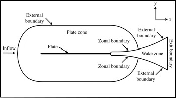
The computational region is divided into two zones to facilitate grid generation and provide adequate grid resolution for the wake. Figure 1 shows the plate cross-section and the two zones that comprise the computational region. The three-dimensional zones and grids are obtained by uniformly spacing copies of these two-dimensional zones in the spanwise direction (
 $z$
).
Midspan plate section and multiple zone discretization of the computational region (Rai Reference Rai2013).

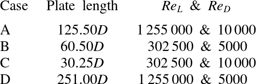
The plate zone is bounded by four boundaries: the plate surface (excluding the trailing edge), an external boundary and two zonal boundaries (top and bottom) that interface with the wake zone. The plate zone captures the inviscid flow field upstream of the trailing edge and the plate boundary layers. The leading edge of the plate is an ellipse. The wake zone is constructed to provide adequate grid resolution for the DSLs, the recirculation region and the wake. The boundaries of this zone include the circular trailing edge, the upper and lower boundaries and the exit boundary. Both the upper and lower boundaries consist of a zonal boundary segment that interfaces with the plate zone and a second segment that serves as an external boundary. Direct numerical simulations for four different combinations of
 $\mathit{Re}_{L}$
(Reynolds number based on plate length) and
 $\mathit{Re}_{D}$
were performed to obtain the data used in this study (Cases A, B, C and D).
The external boundary of the plate zone in all cases is placed approximately
 $50D$
from the plate surface, where
 $D$
is the diameter of the circular trailing edge (
 $D$
is also the thickness of the plate). The length of the plate for each case is provided in table 1. The exit boundary of the wake zone is approximately
 $100D$
from the centre of the circular trailing edge (coordinate system origin), and the vertical extent of this boundary is approximately
 $80D$
. The vertical extent of the wake zone near the trailing edge, where its upper/lower boundaries are horizontal, is large enough to completely contain the wake in all cases (figure 4 in Rai Reference Rai2013 clearly shows the adequacy of this dimension in Case A). The spanwise extent of the region in all cases is
 $4.0D$
. Values of
 $\mathit{Re}_{L}$
and
 $\mathit{Re}_{D}$
were chosen to be the vertices of a rectangle in
 $\mathit{Re}_{L}{-}\mathit{Re}_{D}$
space in the order ACBDA (anticlockwise direction, A corresponds to the upper right-hand corner).
Plate length,
 $\mathit{Re}_{L}$
and
 $\mathit{Re}_{D}$
for Cases A–D.

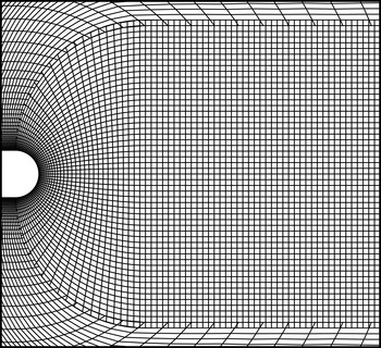
Figure 2 shows representative grids in the vicinity of the trailing edge in both zones. These grids were generated with an algebraic grid generator. Both the grids have the same spacing in the wall-normal direction at the plate surface.
Representative grids in the plate and wake zones in the trailing edge region (Rai Reference Rai2013).

The grid in the wake zone transitions from curvilinear near the trailing edge to rectangular downstream. Downstream of
 $x/D\approx 13.5$
the wake grid coarsens gradually in the
 $x$
direction (in all cases except Case B where grid coarsening begins at
 $x/D=8.5$
). In addition to reducing the computational costs, this coarsening dissipates the wake to such a degree that inviscid exit boundary conditions can be employed at the exit boundary of the wake zone. The wake grid for Case A was constructed with 741 grid points in the streamwise direction, 411 in the cross-stream direction and 256 in the spanwise direction (approximately
 $78\times 10^{6}$
grid points). The resolutions achieved along the centreline in the three spatial directions at
 $x/D=10.0$
are approximately
 ${\rm\Delta}x/{\it\eta}=3.7$
,
 ${\rm\Delta}y/{\it\eta}=2.2$
and
 ${\rm\Delta}z/{\it\eta}=2.1$
, where
 ${\it\eta}$
is the computed Kolmogorov length scale at the same location. The grid resolutions in the plate grid in the
 $x,y$
and
 $z$
directions for this case are approximately 17.8, 0.84 and 6.6 wall units respectively, based on the wall-shear velocity near the end of the plate. The resolutions achieved in all the cases reported here are similar. Additional details are provided in Rai (Reference Rai2013, Reference Rai2014). Cases A and B of the present study are labelled as A and B in Rai (Reference Rai2014) as well.
The high-order accurate upwind-biased method developed in Rai (Reference Rai2008, Reference Rai2010b
) is used here to compute the flow over the plate as well as that in the wake. The inviscid terms are computed using sixth- and seventh-order upwind-biased finite differences, both with seventh-order dissipation terms. The viscous terms are computed with fourth-order central differences. The method is iterative-implicit in nature, multiple iterations are employed at each time step to solve the nonlinear finite-difference equations arising from a fully implicit formulation; the method is second-order accurate in time. As discussed above, the computational region is discretized using the plate grid and the wake grid. The boundaries that contain these grids can be broadly classified as natural and zonal boundaries. The natural boundaries include the external boundary of the plate grid, the surface of the plate, the exit boundary of the wake grid, the segments of the upper and lower boundaries of the wake grid labelled as ‘external boundary’ in figure 1 and the boundaries in the
 $z$
direction. The upstream segment of the upper boundary between the plate and wake grids is an example of the zonal boundaries used in the computation. Periodic boundary conditions are imposed on the boundaries in the
 $z$
direction (homogeneity in
 $z$
). No-slip/adiabatic wall conditions are used on the plate surface. Wall blowing/suction is implemented on a short segment on both the upper and lower surfaces of the plate to induce transition to turbulence. The boundary layer is turbulent upstream of the trailing edge. The upper and lower transitional/turbulent boundary layers and the wake are all computed via DNS. The natural and zonal boundary conditions used here are discussed in Rai (Reference Rai2010b
).
3. Results
The data provided in the following figures were obtained during the data-sampling period (after the initial transients were eliminated). The time step
 $n=0$
corresponds to the time at which sampling was initiated. In the following contour plots the colours blue/green represent negative values (deep blue representing the lowest value) of the term/quantity being discussed. Orange, red and magenta represent positive values (magenta bordering on white representing the highest value). Shades of yellow represent values close to zero. Several aspects of entrainment and the instability of the DSL are discussed in this section. The approach taken here is to use the test case (A, B, C or D) that highlights the attribute that is being discussed, followed as necessary by appropriate remarks regarding the same attribute as it appears in the remaining cases. Velocity statistics etc. were obtained over 160 shedding periods for Cases A and C, and 200 shedding periods for Cases B and D. The time step used in all cases was approximately
 $U{\rm\Delta}T/D=0.0033$
(
 $U$
is the freestream velocity and
 ${\rm\Delta}T$
is the timestep); this corresponds to approximately 1750 time steps per shedding period in Case A.
3.1. Entrainment and assimilation
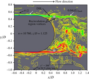
In Rai (Reference Rai2014) it was observed that only a small fraction of the separating turbulent boundary layer participates in the initial roll-up into the shed vortex (approximately
 ${\it\theta}/4$
, where
 ${\it\theta}$
is the momentum thickness of the boundary layer near the trailing edge of the plate). Figure 3 shows contours of spanwise vorticity at one particular instant. The roll-up of the lower shear layer into a shed vortex is marked with a red arrow. The turbulent boundary layer is much thicker than the region depicted by the closely spaced contours corresponding to the DSL. The vertical bar in the figure is
 ${\it\theta}/2$
in length. Here,
 ${\it\theta}$
is the momentum thickness at approximately 94 % plate length. The remarkable feature of the roll-up of the shear layers, which results in the initial formation of the shed vortices, is that only a very small fraction of the turbulent boundary layer participates in this process. Vortical structures in the log layer convect past the trailing edge with relatively little change (for example, the ones in the rectangular box). Thus, fluid adjacent to the shed vortices in the near wake is not irrotational ambient fluid; instead it is turbulent boundary-layer fluid. Consequently, some or all of the fluid that is engulfed by the shed vortices in the near wake is from the separated turbulent boundary layer. The larger the value of
 ${\it\theta}/D$
is, the greater the length of the wake (distance from the trailing edge normalized by
 $D$
) over which the engulfed fluid is boundary-layer fluid and not irrotational ambient fluid. This is in sharp contrast to a low/moderate-Reynolds-number cylinder wake, where the separating boundary layers are laminar.
Instantaneous spanwise vorticity contours (Case A, figure 4 from Rai Reference Rai2014); red/magenta represent high/highest positive values, green/blue low/lowest negative values, yellow
 ${\approx}0.0$
.

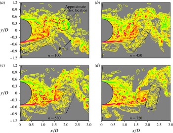
Figure 4(a–d) shows spanwise vorticity contours at four time instants for Case C. The specified minimum and maximum contour levels and the increment between subsequent contour levels are the same in these figures. The rectangular box in each figure shows a set of log-layer eddies convecting downstream and also being assimilated by the rotational flows associated with the lower shed vortex that is just forming (positive) and the more mature upper shed vortex (negative, highlighted with a circle in figure 4
a). The revolving motion of these eddies is clear from the orientation of the box (nearly horizontal in figure 4(a) to nearly vertical in figure 4
d). For the most part the eddies retain their original structure; many of them can be individually identified in these figures. Figure 4(b) shows a few of them merging with the braid and figure 4(d) shows some of them merging with the lower positive shed vortex. The word ‘assimilated’ is used here deliberately; we retain the word ‘entrainment’ for the more conventional process of the advancement of wake turbulence into irrotational ambient flow (as, for example, in Townsend (Reference Townsend1966)). Figure 4(c,d) shows eddies in the region
 $-1.2\leqslant y/D\leqslant -0.8$
that are more distant from the shed vortices and hence will travel further downstream before being similarly assimilated. It is evident in figures 3 and 4 that the shed vortex is not a single cylindrical vortex as in low-Reynolds-number shedding. Instead, it is an amalgam of several smaller vortices of both signs (with vortices of the same sign as the vorticity in the shear layer that is rolling up dominating), segments of the shear layer and shear-layer vortices. This point has been made in Rai (Reference Rai2013, Reference Rai2014) but is repeated here to stress the complexity of shed-vortex structure.
Instantaneous spanwise vorticity contours showing assimilation of log-layer eddies at (a)
 $T/T_{p}=0.066$
, (b)
 $T/T_{p}=0.298$
, (c)
 $T/T_{p}=0.384$
and (d)
 $T/T_{p}=0.477$
(Case C, shedding period
 $T_{p}$
); red/magenta represent high/highest positive values, green/blue low/lowest negative values, yellow
 ${\approx}0.0$
.

The emphasis in this study is on cases where
 ${\it\theta}/D$
is small (less than 0.5) and the log layer and the outermost part of the separated boundary layer as well are engulfed by the rotational motion of the shed vortices. In cases where
 ${\it\theta}/D$
is significantly larger, shedding is expected to be weaker and perhaps non-existent, thus resulting in thin-plate wake physics investigated in numerous studies, one of the earliest being that of Chevray & Kovaznay (Reference Chevray and Kovaznay1969). Entrainment there is perhaps of the kind discussed in Townsend (Reference Townsend1966) and may exist in the present situation as well in the outer parts of the separated boundary layer before it gets assimilated. Case D (largest value of
 ${\it\theta}/D$
computed here), discussed below (figure 5
c), is a case in point.
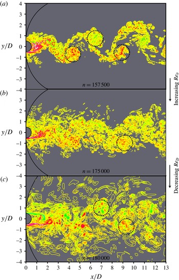
Instantaneous spanwise vorticity contours: (a) Case C, (b) Case A, (c) Case D; red/magenta represent high/highest positive values, green/blue low/lowest negative values, yellow
 ${\approx}0.0$
.

Figure 5(a–c) shows instantaneous spanwise vorticity contours for Cases C, A and D respectively. The approximate locations of the shed vortices are marked with circles. The specified minimum and maximum contour levels and the increment between subsequent contour levels are the same in these figures. In the following discussion and later in this section Case A is used as the reference; all other cases considered are deviations in terms of
 ${\it\theta}$
and/or
 $D$
. In Case C (figure 5
a,
 ${\it\theta}$
is approximately a third of Case A while
 $D$
is the same) most of the assimilation has occurred by
 $x/D=5$
; thereafter the distinction between braids and vortices is clear; only a few eddies are not associated with these entities.
Past
 $x/D=5$
we have more conventional entrainment where irrotational ambient fluid is engulfed, but by rib vortices in the braids (figure 8 in Rai Reference Rai2013) and those wrapped around shed vortices and also by elongated spanwise vortices in the peripheral regions of the shed vortices (figure 11 in Rai Reference Rai2013).
In Case D (figure 5
c,
 ${\it\theta}$
is approximately the same as in Case A but D is half as large) eddies from the boundary layer persist until
 $x/D=13$
, and so assimilation of these structures continues until this location in the computation and even beyond. It is difficult to visually locate the braids and vortices in Case D because of the vortical clutter. In figure 5(b) (Case A) we have a situation that is in between the two extreme cases discussed above. Assimilation of boundary-layer vortical structures is essentially complete by approximately
 $x/D=10$
, and thereafter, for the most part, we have entrainment of irrotational ambient fluid. Hence, decreasing
 ${\it\theta}$
or increasing
 $D$
shortens the region of the wake, in terms of streamwise distance normalized by
 $D$
, where boundary-layer fluid is assimilated by the shed vortices (and braids).
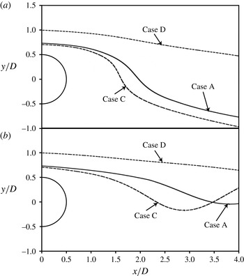
To better illustrate the rapid assimilation of boundary-layer fluid in Case C and the slow assimilation in Case D (relative to Case A), figure 6 shows particle traces obtained in each of these cases.
Particle traces obtained for Cases C, A and D, with traces initiated at (a)
 ${\it\phi}=0.00$
and (b)
 ${\it\phi}=0.52$
.

The phase-averaged velocity fields (velocity components are a function of shedding phase
 ${\it\phi}$
) were used for this purpose. The traces were all initiated in the log layer at very nearly
 $y^{+}=100$
(wall-shear velocity as obtained at 90 % plate length). Different values of
 $y/D$
are obtained at the trace origination points (left boundary of figure 6) in the three cases because of different wall-shear velocities and plate thicknesses. The plate thickness in Cases A and C is the same, while the wall-shear velocity in Case C is higher than in Case A (shorter plate length). In Cases A and D the wall-shear velocity is approximately the same whereas the plate thickness in Case D is half of that in Case A. The latter feature results in the initial
 $y/D$
value being substantially higher in Case D (the location of the log layer is further away from the wall and its extent is larger in terms of the plate thickness in Case D).
The initial phase value (trace initiation) in figure 6(a) is
 ${\it\phi}=0.00$
, and in figure 6(b) it is
 ${\it\phi}=0.52$
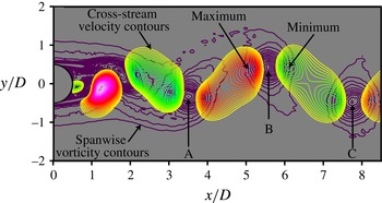
. The centre of one of the upper vortices (vortex B in figure 7) is located at
 $x/D=5.5$
at
 ${\it\phi}=0.00$
. Details of the phase-averaging procedure are provided in Rai (Reference Rai2013). It is clear from figure 6(a) that log-layer assimilation in Case C is more rapid than in Case A; this is a result of both a slightly lower particle release location as well as stronger shed vortices in Case C (shed-vortex strength is discussed below). Both traces dip below the wake centreline. The trace obtained in Case D shows only a slight movement towards the centreline, thus indicating a much slower assimilation rate than both Cases A and C. The same relative trends are seen in figure 6(b) as well (traces initiated near the middle of the shedding period).
Phase-averaged contours of spanwise vorticity (magenta) in the background and cross-stream velocity in the foreground (Case C,
 ${\it\phi}=0$
); red/magenta represent high/highest positive values, green/blue low/lowest negative values, yellow
 ${\approx}0.0$
.

The thickness of the boundary layer in relation to
 $D$
is one of the important factors affecting the rapidity of assimilation; the thicker the boundary layer is in relation to the cross-stream extent of the engulfing mechanism (in this case the shed vortices which extend over a region of approximately one diameter in the
 $y$
direction in the very near wake) the longer it takes to be assimilated. However, one wonders whether there are other factors that play a role as well. Figure 7 shows contours of phase-averaged cross-stream velocity superimposed on contours of phase-averaged spanwise vorticity at the phase
 ${\it\phi}=0.00$
.
Figure 7 shows two lobes (velocity contours), one on either side of vortex B. The lobes show peak values on the left and right of B; on the left we have an upward flow and on the right a downward flow. These cross-stream flows are vortex induced. The upward flow on the left of vortex B is, for example, induced by vortices A and B. The magnitudes of the peak values in cross-stream velocity are determined by the strength of the vortices. Since vortex strength diminishes with increasing
 $x/D$
, the peak cross-stream velocity on the upstream side of a vortex is larger in magnitude than that on the downstream side. The ratio of peak cross-stream velocity magnitudes in this case (left to right, vortex B) is 1.14. The colour scheme indicates increasing peak velocity values with decreasing
 $x/D$
; the most powerful upward flow in figure 7 is on the right of the positive vortex that has just formed (centre at approximately
 $x/D=1.0$
).
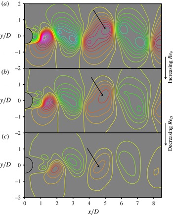
Figure 8(a–c) shows contours of the phase-averaged cross-stream velocity for Cases C, A and D respectively (all at
 ${\it\phi}=0.00$
). The specified minimum and maximum contour levels and the increment between subsequent contour levels are the same in these figures.
Contours of phase-averaged cross-stream velocity (
 ${\it\phi}=0$
): (a) Case C, (b) Case A, (c) Case D; red/magenta represent high/highest positive values, green/blue low/lowest negative values, yellow
 ${\approx}0.0$
.

The arrows point to locations where the peak positive values occur to the left of the vortices at
 $x/D=5.5$
. While figure 8(a) shows two peaks per lobe for all lobes except the two associated with the positive vortex that has just formed, figures 8(b) and 8(c) only have one peak per lobe. The ratio of the positive peak velocity values on the left of the vortices at
 $x/D=5.5$
in figure 8(a–c) is 1.58:1.00:0.68, thus peak velocity decreases with increasing
 ${\it\theta}$
and decreasing
 $D$
. This is consistent with the decreasing peak vorticity levels with increasing
 ${\it\theta}$
and decreasing
 $D$
. The ratio of peak vorticity levels for cases C, A and D (at
 $x/D=5.5$
) is 1.65:1.00:0.58 (vorticity as normalized by
 $U/D$
, where
 $U$
is the free stream velocity,
 $U$
is the same for all cases). Thus, a boundary layer that is thick (in relation to
 $D$
) results in weaker shed vortices. This is another reason why assimilation is more effective in Case C than in Case D: Case D has substantially weaker vortices and thus weaker cross-stream flows. A power-law relationship between peak phase-averaged spanwise vorticity within vortex cores (when they occupy the streamwise location
 $x/D=5.5$
) and
 $\mathit{Re}_{{\it\theta}}$
at separation and
 $\mathit{Re}_{D}$
is provided in appendix A.
The continued presence of boundary-layer vortical structures at values of
 $x/D$
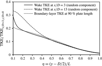
as large as 13.0 leads to the following question: do the velocity statistics of the boundary layer persist in the wake region at cross-stream locations that are removed from shed vortices and braids? Figure 9 shows profiles of the fluctuating kinetic energy (random component only, or TKE) for Case D at the locations
 $x/D=3.0$
and 13.0. The TKE data are normalized with the TKE value at
 $x/D=3.0$
on the wake centreline. The boundary-layer TKE profile (total) at 90 % plate length is also shown in this figure. The contribution from any periodic component is expected to be small because this
 $x$
location is approximately
 $25D$
upstream of the trailing edge.
Profiles of TKE in the boundary layer and wake for Case D.

Because the boundary layer exists only for
 $y/D\geqslant 0.5$
(the wake centreline is at
 $y/D=0.0$
), the TKE data are shown as a function of
 ${\it\eta}=(y-D/2)/L$
, where
 $L$
is a reference length (approximately the boundary-layer thickness). The wake profile at
 $x/D=3.0$
is almost the same as the boundary-layer profile from
 ${\it\eta}\approx 0.2$
onwards (most of the boundary layer). The boundary-layer TKE distribution is preserved even at the location
 $x/D=13.0$
for
 ${\it\eta}\geqslant 0.45$
. The turbulent nature of the boundary layer results in a preservation of boundary-layer properties well into the wake region for large values of
 ${\it\theta}/D$
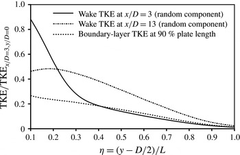
. In contrast, in the case of the cylinder with laminar separating boundary layers, much of the boundary layer rolls up into shed vortices after separation (figure 26, Rai Reference Rai2014). Figure 10 shows profiles of TKE for Case A (smaller value of
 ${\it\theta}/D$
). Here, at
 $x/D=3.0$
the boundary-layer profile is preserved only for
 ${\it\eta}\geqslant 0.4$
. At
 $x/D=13.0$
there is little resemblance between the wake and boundary-layer profiles, implying that the assimilation of boundary-layer fluid is complete at this
 $x$
location. The trend seen in figures 9 and 10 (continued assimilation of boundary-layer fluid at larger values of
 $x/D$
with increasing
 ${\it\theta}/D$
) is consistent with the trend in figure 5(a–c).
Profiles of TKE in the boundary layer and wake for Case A.

Contours of the turbulent transport term in the transport equation for the phase-averaged TKE (coloured contours), and phase-averaged pressure contours (magenta, dashed lines) for Case A (
 ${\it\phi}=0$
); red/magenta represent high/highest positive values, green/blue low/lowest negative values, yellow
 ${\approx}0.0$
.

While some of the discussion above focused on assimilation/entrainment in an instantaneous sense, is there an effective way of understanding this process in a phase-averaged sense in the present situation? The turbulent transport terms in the transport equation for the phase-averaged turbulent stresses (random component) are given by (assuming incompressible flow, Rai Reference Rai2012)
 $$\begin{eqnarray}T_{ij}=-{\it\rho}\left(\frac{\partial \langle u_{i}^{\prime }u_{j}^{\prime }u_{k}^{\prime }\rangle }{\partial x_{k}}\right).\end{eqnarray}$$
Here,
 ${\it\rho}$
is the density,
 $u_{i}^{\prime }~(i=1,2,3)$
are the fluctuating velocity components (random) in the
 $x$
,
 $y$
and
 $z$
directions (
 $x_{i}$
), repeated indices denote summation, and bracketing of any flow variable by
 $\langle \,\rangle$
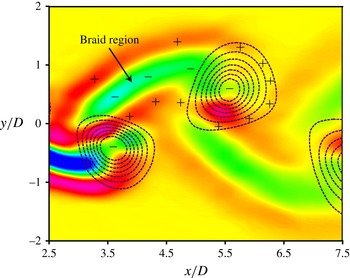
represents phase averaging of the variable. Figure 11 shows the distribution of the turbulent transport term in the transport equation for the phase-averaged TKE (Case A,
 $T_{mm}/2$
) at the phase
 ${\it\phi}=0.00$
. Figure 11 also shows contours of the phase-averaged pressure (magenta, dashed lines) at
 ${\it\phi}=0.00$
so that the shed vortices and their centres can be easily located. The ‘
 $+$
’ and ‘
 $-$
’ signs and the colour scheme provide the sign of the transport term; positive values represent transport of TKE into a region and negative values represent transport out of a region. The distribution of figure 11 represents the ‘averaged or net transport rate’ (in a phase-averaged sense) and not the instantaneous transport rate of TKE.
Figure 11 shows transport of TKE out of the central braid region where we have large values for the production of phase-averaged TKE (figure 7, Rai Reference Rai2013 shows the distribution of the production term). The TKE is transported both above and below the central braid region, creating three distinct layers that define the braid (one negative and two positive). The distribution of the transport term in the shed-vortex region is more complicated. We have transport out of the central region and transport into most of the region surrounding the vortex core except where the braid merges with the vortex core; here once again the transport term is negative. The increase in the area of negative transport (comparing corresponding regions) with increasing
 $x/D$
is evident. This represents a corresponding increase in size of the braid regions that is sustained for the remaining well-resolved portion of the wake (
 $x/D\approx 13.5$
). Figure 11 shows that much of the transport of TKE into the surrounding flow is associated with the braids and not the vortex cores.
As seen in figures 4 and 5, log-layer eddies that are assimilated occur above the braid regions in the upper half of the (
 $x,y$
) plane and below these regions in the lower half of the plane. These eddies are also found in the ‘v’ shaped regions between shed vortices of the same sign where fluid is engulfed because of the rotational motion (clearly seen in figure 4
c). Figure 11 shows the phase-averaged turbulent transport term to be positive in all these regions occupied by log-layer eddies. That is, in a phase-averaged sense, turbulence is transported from the braids and shed vortices into the adjacent separated boundary layer. Powerful rib vortices in the braids and those wrapped around the vortex cores, and also elongated spanwise vortices in the peripheral regions of the shed vortices mentioned earlier, are the most probable cause for the net turbulence transport away from the braids and cores. Interestingly, even though the log-layer eddies are assimilated by the braids and cores, the net transport of turbulence is outward from these braids and cores.
3.2. Instability of the detached shear layers
3.2.1. Shear-layer characteristics
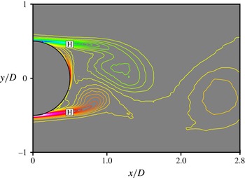
The computed pressure and velocity components at the points marked with an ‘H’ in figure 3 were stored during the sampling period. As discussed in Rai (Reference Rai2014), the incoming velocity fluctuations from the upstream turbulent boundary layer are large and thus do not exhibit a spectral broadband peak because of shear-layer vortex generation. However, the pressure fluctuations that are a result of shear-layer vortices are sufficiently large in comparison with boundary-layer pressure fluctuations. A spectral analysis of the pressure fluctuations at the points marked ‘H’ in Rai (Reference Rai2014) does show a broadband peak in addition to a sharp one at the shedding frequency.
Figure 12 shows the pressure data obtained in a (
 $t,z$
) plane in the upper and lower shear layers over 10 shedding periods at the ‘H’ points for Case C (a similar plot for Case A is provided in Rai Reference Rai2014). The entire spanwise extent of the computational region (
 $4.0D$
) was used to obtain figure 12. The pressure data plotted here were obtained from a high-pass filter applied to the original computed data. The filter was used to eliminate the effect of periodic shedding. The cutoff frequency was set at
 $2.4{\it\omega}_{st}$
; this is higher than the
 $1.5{\it\omega}_{st}$
used in Rai (Reference Rai2014) because of the presence of a small but sharp peak at
 $2.0{\it\omega}_{st}$
in the computed spectrum for Case C (periodic shedding-related component).
Contours of filtered fluctuating pressure in a (
 $t,z$
) plane in both shear layers (Case C); red/magenta represent high/highest positive values, green/blue low/lowest negative values, yellow
 ${\approx}0.0$
.

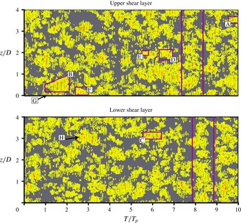
Numerous intermittency events and quiescent periods are evident in both the upper and lower shear layers in figure 12. Every event consists of a few or several vertical bands, each band in the blue/green range or red/orange range. The former set of bands is a result of the pressure minima caused by the passing shear-layer vortices and the latter set represents a recovery of the pressure that occurs between subsequent shear-layer vortices. The vertical lines (magenta) and instability events highlighted in figure 12 (A, B, C, D, E, F, G and H) are used in the following subsections to better understand various attributes of the DSLs such as (a) variation in shear-layer vortex generation rates from event to event, (b) the generation of shear-layer vortices by log-layer eddies and (c) a variation in the prevalence and intensity of shear-layer vortices with shedding phase.
3.2.2. Variation in shear-layer vortex generation rates
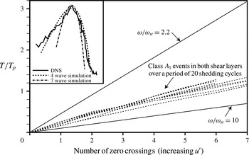
Figure 13 is reproduced from Rai (Reference Rai2010a
). It shows the zero crossings (dashed lines) in the fluctuating velocity signal obtained in the vicinity of the shear layers of a cylinder at
 $\mathit{Re}_{D}=3900$
during powerful intermittency periods (labelled as Class
 $A_{1}$
there). The upper and lower bold lines (
 $2.2{\it\omega}_{st}$
and
 $10.0{\it\omega}_{st}$
) represent the left and right extents of the broadband peak that appears in the velocity spectrum because of the shear-layer instability. The point is made in Rai (Reference Rai2010a
) that the zero crossing lines are clustered together and are distant from the lines corresponding to the left and right extents of the broadband peak. Thus, the shear-layer vortex generation rate does not show the variability that the broadband peak suggests. The point is also made there that the broadband nature of the peak is most probably because of signal modulation (increasing amplitude in the first half of an instability event followed by decreasing amplitude in the second half of the event). The inset in figure 13 shows the computed broadband peak for the cylinder and the peaks obtained for simple single-frequency simulated waves that have undergone modulation, and the agreement between the two.
Times at which zero crossings occur in the
 $u^{\prime }$
signal for Class
 $A_{1}$
events in the upper and lower shear layers over 20 shedding cycles for the cylinder at
 $\mathit{Re}_{D}=3900$
(figure 26, Rai Reference Rai2010a
).

Instantaneous contours of filtered fluctuating pressure in a (
 $t,z$
) plane (Case C) showing (a) Event B and (b) Event D; red/magenta represent high/highest positive values, green/blue low/lowest negative values, yellow
 ${\approx}0.0$
.

The variation in shear-layer vortex generation rate obtained for the numerous instability events portrayed in figure 13 is approximately
 $\pm 15\,\%$
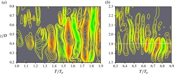
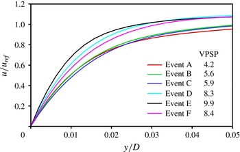
. The variation in the case of the flat plate is larger. Figure 14 shows an enlarged view of events B and D from figure 12. Contour lines close to zero have been omitted in this figure to clearly show the separation between bands. The majority of the bands in figure 14(a) are much wider than those in figure 14(b). There are five pairs of bands (each pair corresponding to the passage of one shear-layer vortex and the accompanying pressure recovery) over a period of 0.9 shedding periods in figure 14(a), that is, a vortex generation rate of approximately 5.6 vortices per shedding period (VPSP). Similar computations for events A, C, D, E and F yield the rates 4.2, 5.9, 8.3, 9.9 and 8.4 VPSP respectively. Thus, the vortex generation rate varies by more than a factor of 2.0 in just the few events that were inspected (not an exhaustive search). Here, we seek the reason behind these differences in vortex generation rates from event to event. Broadening of the spectral peak (associated with the shear-layer instability) because of amplitude modulation is expected in addition to this variation in shear-layer vortex generation rate.
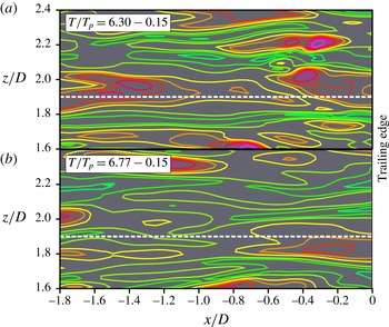
Figure 15(a,b) shows near-wall contours (upper plate surface,
 $y-y_{wall}=0.00846D$
) of fluctuating streamwise velocity (instantaneous velocity – time-averaged velocity at a given
 $x$
and
 $y$
location) upstream of the trailing edge at two instants in time.
Near-wall contours of fluctuating streamwise velocity upstream of the trailing edge (Case C): (a)
 $T/T_{p}=6.15$
, (b)
 $T/T_{p}=6.62$
; red/magenta represent high/highest positive values, green/blue low/lowest negative values, yellow
 ${\approx}0.0$
.

The streamwise extent of these plots is
 $1.8D$
;
 $x/D=0.0$
corresponds to the location of the centre of the circular trailing edge. In the
 $z$
direction the plots extend from
 $z/D=1.6$
to 2.4. The horizontal dashed line in figure 14(b) is located at
 $z/D=1.9$
; it approximately cuts through the centre of the bands that comprise the instability. The spanwise extent in figure 15(a,b) was chosen to contain the location
 $z/D=1.9$
well within the plotted area. The time instant chosen for figure 15(a) is
 $T/T_{p}=6.3-0.15$
(
 $T$
is the time and
 $T_{p}$
is the shedding period). The first component on the right-hand side (6.3) corresponds to the inception of instability event D (
 $T/T_{p}=6.3$
). The second component (0.15) is the estimated time taken for the fluctuating velocity distribution seen in figure 15(a) to arrive at the location
 $x/D=0.5$
at which pressure values are stored (the points marked H in figure 3). In other words, the leading edge of the fluctuating velocity distribution (
 $x/D=0.0$
) at
 $T/T_{p}=6.15$
arrives at
 $x/D=0.5$
at
 $T/T_{p}=6.3$
. The estimate of the time delay was obtained by tracking maxima in the fluctuating velocity distribution, in the vicinity of
 $z/D=1.9$
, in time.
Figure 15(a) shows a high-speed streak extending both above and below
 $z/D=1.9$
(white dashed line) that convects over the point H in the upper shear layer over the entire period of Event D. Figure 15(b) is similar to figure 15(a) but corresponds approximately to the end of the instability in figure 14(b) (the leading edge of the velocity distribution arrives over H at
 $T/T_{p}=6.77$
). Events E and F were also accompanied by a high-speed streak, whereas Events A, B and C corresponded to a mixed velocity distribution. Given that the velocity distribution in high-speed streaks is on average (conditional mean) higher than that obtained in the time-mean velocity distribution, we have one possible candidate to explain the higher vortex generation rate seen in Event D, i.e. higher than average values of velocity (assuming, as in Bloor Reference Bloor1964, that
 ${\it\omega}_{sl}$
is proportional to a characteristic velocity
 ${\it\upsilon}$
divided by a length
 ${\it\lambda}$
). A second possibility is a corresponding thinning of the DSL (a decrease in
 ${\it\lambda}$
). However, first, a quantitative measure of increased (or decreased) velocities in the turbulent boundary layer is desirable. Here, we use a conditional averaging technique to obtain one. The mean velocity distribution associated with an event is computed by averaging the streamwise velocity over the area corresponding to the event seen in figure 12. The time period for averaging takes into account the time delay for the event, as explained previously. The delays were slightly different for each of the events highlighted in figure 12.
Figure 16 shows the velocity profiles thus obtained for these events, at
 $x/D=0.0$
. Events A, B and C have profiles that are close to each other and lower than the rest of the profiles; the corresponding vortex generation rates are between 4.2 and 5.9 VPSP. Events D, E and F have profiles that are higher than those of A, B and C, and vortex generation rates between 8.3 and 9.9 VPSP.
Velocity profiles associated with Events A, B, C, D, E and F obtained via a conditional averaging technique at
 $x/D=0.0$
(Case C).

Thus, velocity fluctuations in the turbulent boundary layer corresponding to sizeable features, such as high-speed streaks, seem to have a substantial effect on shear-layer vortex generation rates. Ultimately, one would like to have a measure of shear-layer thickness in addition to local velocity during an event.
3.2.3. Generation of shear-layer vortices by log-layer eddies
The destabilization of the DSL by recirculation region vortices in the case of the cylinder (laminar separating boundary layers) is discussed in Rai (Reference Rai2010a ). The results of Rai (Reference Rai2014) strongly indicate that the interaction of the DSL with recirculation region vortices is an important contributor to the instability of the DSL in the case of the flat plate with turbulent separating boundary layers as well. Here, we explore the possibility of the log-layer vortices in the proximity of the DSL, convecting past the trailing edge essentially unchanged, contributing to the generation of shear-layer vortices. We also investigate underlying mechanisms of generation.
Instantaneous spanwise vorticity contours showing the interaction of the shear layer with log-layer eddies: (a)
 $n=8230$
and (b)
 $n=8340$
(Case C, Event E,
 $z/D=1.98$
); red/magenta represent high/highest positive values, green/blue low/lowest negative values, yellow
 ${\approx}0.0$
.

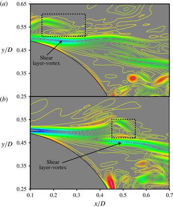
Figure 17(a,b) shows spanwise vorticity contours at two instants in time. Both instants are from the event marked E in figure 12. In figure 17(a) we have a cluster of log-layer eddies (in the rectangular box) interacting with the upper shear layer. This figure also shows the inception of a shear-layer vortex. Figure 17(b) (110 time steps later) shows the same shear-layer vortex further downstream. Thus, log-layer eddies seem to play a role in the evolution of shear-layer vortices. The cluster of log-layer eddies in figure 17(b) is further downstream in relation to the shear-layer vortex. This phenomenon was observed at other times when log-layer eddies were associated with shear-layer vortices. This is unlike cases where recirculation region vortices are the most likely cause for destabilization (the prevalent mode). There, because of low convection velocities in the recirculation region (both forward and reverse flow), vortices of this region interact with a particular area of the shear layer for longer periods. A few relatively powerful shear-layer vortices are generated during such periods. Log-layer eddies are usually associated with the evolution of only one shear-layer vortex; they convect downstream along with this vortex and subsequently move downstream of the recirculation region. The powerful shear-layer vortices sometimes obtained when recirculation region vortices are the likely cause are rarely found when log-layer eddies alone interact with the shear layer. It was also observed that an instability event can be associated with both log-layer eddies and recirculation region vortices. In such cases the potentially productive period of interaction of the shear layer with log-layer eddies typically occurs at the beginning of the instability event.
Consider the inviscid incompressible form of the transport equation for spanwise vorticity:
 $$\begin{eqnarray}\left.\begin{array}{@{}c@{}}\displaystyle \frac{\text{D}{\it\omega}_{z}}{\text{D}t}=T_{T},\\ T_{T}=T_{1}+T_{2}+T_{3},\\ \displaystyle T_{1}={\it\omega}_{x}\frac{\partial w}{\partial x};\quad T_{2}={\it\omega}_{y}\frac{\partial w}{\partial y};\quad T_{3}={\it\omega}_{z}\frac{\partial w}{\partial z}.\end{array}\right\}\end{eqnarray}$$
Here,
 ${\it\omega}_{x},{\it\omega}_{y}$
and
 ${\it\omega}_{z}$
are the components of vorticity in the
 $x$
,
 $y$
and
 $z$
directions respectively and
 $w$
is the spanwise component of velocity. Assuming that the shear layer is initially quiescent and essentially two-dimensional yields
 ${\it\omega}_{x}={\it\omega}_{y}=0$
, and the above equation reduces to
 $$\begin{eqnarray}\frac{\text{D}{\it\omega}_{z}}{\text{D}t}={\it\omega}_{z}\frac{\partial w}{\partial z}.\end{eqnarray}$$
In the cylinder case (Rai Reference Rai2010a
) it was found that the interaction of the shear layer and recirculation region vortices results in an efflux of fluid away from the region of interaction, causing the local value of the derivative of the spanwise velocity in the
 $z$
direction,
 $\partial w/\partial z$
, to become positive. This positive value of
 $\partial w/\partial z$
results in production of
 ${\it\omega}_{z}$
and shear-layer vortices (according to (3.3)). These vortices are essentially oriented with the
 $z$
direction initially. They appear on the ridges caused by the interaction of the shear layer with recirculation region vortices. The development of
 ${\it\omega}_{x}$
that occurs shortly thereafter in the valleys on either side of a ridge results in crescent shaped shear-layer vortices; this is also discussed in Rai (Reference Rai2010a
) utilizing the vorticity transport equation for
 ${\it\omega}_{x}$
.
While the reasoning in the case of a cylinder is relatively straightforward, the existence of complex distributions of
 ${\it\omega}_{x}$
and
 ${\it\omega}_{y}$
in a separating turbulent boundary layer makes a similar analysis formidable. Instead, the instantaneous distributions of the terms on the right-hand side of (3.2) were investigated. It was found that the term
 $T_{2}$
was the dominant contributor to an increase in the magnitude of the local value of spanwise vorticity in the vicinity of the shear-layer vortex at
 $n=8230$
(time instant corresponding to figure 17
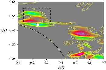
a). Figure 18 shows the distribution of this term at that instant. The cluster of log-layer eddies above the shear layer (in the rectangular box) and the region where
 $T_{2}$
is negative (just below this cluster) are evident. The centre of the shear-layer vortex is marked with an ‘x’ in this figure. The peak negative value of
 $T_{2}$
in this region occurs close to the centre of the shear-layer vortex. It was observed that
 $T_{T}$
was negative as well in the vicinity of the shear-layer vortex. We note here that negative values of
 $T_{T}$
correspond to production of vorticity of the same sign as the vorticity associated with the upper shear layer. The peak value of
 $T_{T}$
was found to occur slightly downstream of the point ‘x’. The shear-layer vortex and the negative peak in
 $T_{T}$
maintained their relative positions with respect to each other as they travelled downstream. The terms
 $T_{1}$
and
 $T_{3}$
are both positive in the region of the point marked ‘x’; this simplifies the search for the reasons underlying shear-layer vortex inception in this particular case. We simply look at instantaneous distributions of the contributors to the term
 $T_{2}$
at the time instant in question (
 ${\it\omega}_{y}$
and
 $\partial w/\partial y$
). This is because only
 $T_{2}$
contributes to a local increase in the magnitude of
 ${\it\omega}_{z}$
.
Instantaneous distribution of
 $T_{2}$
at
 $n=8230$
, (Case C, Event E); red/magenta represent high/highest positive values, green/blue low/lowest negative values, yellow
 ${\approx}0.0$
.

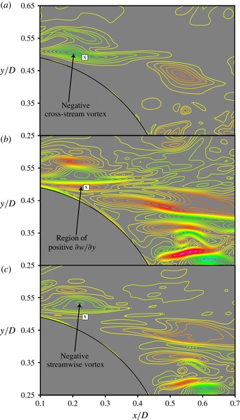
Figures 19(a) and 19(b) show the instantaneous distribution of
 ${\it\omega}_{y}$
and
 $\partial w/\partial y$
respectively, at the time instant
 $n=8230$
. The centre of the shear-layer vortex is marked with an ‘x’ in both these figures. In the region of the point ‘x’ we have a negative cross-stream vortex (figure 19
a) and positive values of
 $\partial w/\partial y$
(figure 19
b). The product of the two is negative; thus we obtain the negative values of
 $T_{2}$
in the region of the shear-layer vortex as seen in figure 18. We now seek the underlying reason for the region of positive
 $\partial w/\partial y$
seen in figure 19(b). Figure 19(c) shows the distribution of
 ${\it\omega}_{x}$
at the same time instant as in figure 19(a,b). The negative streamwise vortex in the log layer located above the shear-layer vortex is evident. The streamwise vortex induces a positive spanwise velocity field that first increases in magnitude with decreasing
 $y$
(starting at the core of this vortex) and then decreases in magnitude (in the absence of other extraneous effects). This results in the region of negative
 $\partial w/\partial y$
just below the streamwise vortex and a region of positive
 $\partial w/\partial y$
further down near the centre of the shear-layer vortex. Thus, we have the cross-stream vortex (figure 19
a) that, for the most part, is located in the shear layer and the streamwise vortex (figure 19
c) in the log layer interacting to generate a shear-layer vortex.
Instantaneous contours of (a)
 ${\it\omega}_{y}$
, (b)
 $\partial w/\partial y$
and (c)
 ${\it\omega}_{x}$
(
 $n=8230$
, Case C, Event E); red/magenta represent high/highest positive values, green/blue low/lowest negative values, yellow
 ${\approx}0.0$
.

The event described above is certainly not an isolated event. For example, the region labelled as ‘G’ in figure 12 also showed the generation of a shear-layer vortex in the absence of an interaction of the shear layer with recirculation region vortices. Log-layer eddies and eddies in the DSL were determined to be the cause. The term
 $T_{2}$
was found to cause the inception of the shear-layer vortex as in Event E. However, the magnitude of the term
 $T_{3}$
(negative) increased substantially as the cluster of log-layer eddies travelled downstream. One particular log-layer streamwise vortex resulted in efflux away from the region of interaction (as in the case of the cylinder, Rai Reference Rai2010a
) and consequently caused the growth of
 $T_{3}$
and also strengthened the shear-layer vortex. While the details of the shear-layer vortex generation process vary somewhat from event to event, the common theme is an interaction of vortices in the shear layer and log layer. It should be noted that a region of negative cross-stream vorticity, not necessarily a cross-stream vortex as in figure 19(a), may also generate the region of negative
 $T_{2}$
seen in figure 18.
As seen above, a cluster of log-layer eddies, because of its rapid convection rate, is usually only responsible for one shear-layer vortex. One or more recirculation region vortices, interacting with the shear layer at approximately the same time, may generate a few shear-layer vortices in succession. Recirculation region vortices are the primary contributor to the instability process. They have been observed to both initiate the generation of shear-layer vortices and strengthen them. Their interaction with the DSL and the shear-layer vortices can at times be very complex, with several of them working in unison to destabilize the DSL.
Instantaneous spanwise vorticity contours showing the interaction of the shear layer with recirculation region vortices: (a)
 $n=3730$
and (b)
 $n=3990$
(Case C, Event H,
 $z/D=3.03$
); red/magenta represent high/highest positive values, green/blue low/lowest negative values, yellow
 ${\approx}0.0$
.

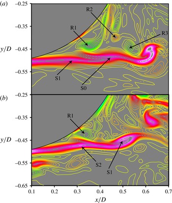
Figure 20(a,b), showing instantaneous spanwise vorticity contours, illustrates a relatively simple interaction between recirculation vortices and the shear layer. Figure 20(a) shows three recirculation region vortices (R1, R2 and R3) and two shear-layer vortices (S0 and S1). The vortex S0 is well formed and is a consequence of the interaction between R1 and the shear layer at an earlier instant. Of interest is the inception of S1 because of the interaction between R1 and the shear layer, around the time period
 $n=3730$
(figure 20
a). A few time steps later (
 $n=3990$
), R1 continues to be a distinct vortex but R2 and R3 seem to have merged with the shear layer. The vortex S1, because of its interaction with R1, R2 and R3, has strengthened and grown in size. The continued interaction of R1 with the shear layer results in the inception of a third shear-layer vortex, S2. Thus, one or more recirculation region vortices remaining mostly in one location may generate several shear-layer vortices. The major contributor to the inception of both S1 and S2 was the term
 $T_{3}$
in (3.2) (efflux of fluid in the
 $z$
direction away from the region of interaction).
3.2.4. Shear-layer vortex generation and shedding phase
An inspection of figure 12 shows that there are short periods in time during which the shear-layer instability is essentially absent over the entire spanwise extent of the computational domain. Some of these periods are marked with vertical lines (magenta) in both the upper and lower shear layers in figure 12. The lines are very nearly one shedding period apart in a given shear layer. The lines in the upper shear layer are displaced by approximately half a shedding period from those in the lower shear layer. The following analysis was performed to determine whether indeed shear-layer vortex generation is related to the phase of shed vortices. We note that any resulting periodicity is different from that obtained directly from the shedding itself (sharp peak in the spectrum at the shedding frequency). The filtered fluctuating signal at each
 $z$
location was squared and then summed in the
 $z$
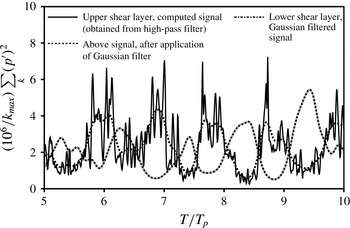
direction. Figure 21 shows the resulting signal obtained in the upper shear layer over five shedding periods. While this signal itself shows shedding-phase dependence in the generation of shear-layer vortices (the low points in the signal indicate times when the shear layer is relatively quiescent), the computed signal is rather noisy. A Gaussian filter was applied to this signal to reduce the high-frequency fluctuations. Figure 21 shows the resulting signal obtained in the upper and lower shear layers. Periodicity in the shear-layer vortex generation process is evident; so is the shift of approximately half a shedding period between the signals of the upper and lower shear layers.
Signals obtained from processing the data of figure 12 (Case C).

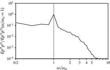
Figure 22 shows the spectrum of the signals obtained after the application of the Gaussian filter (the spectra obtained from the upper and lower shear layers were averaged to obtain the spectrum shown in this figure). The sharp peak at
 ${\it\omega}/{\it\omega}_{st}=1$
is evident. Thus, shear-layer vortex generation peaks and subsides on average, at the shedding frequency. This indicates an interaction between the large-scale shed vortices and the small-scale shear-layer vortices. Here, we seek the underlying physical mechanism.
Spectrum of the
 $z$
-averaged kernel-smoothed signal (upper and lower shear-layer spectra averaged, Case C).

Figure 23 shows phase-averaged spanwise vorticity contours at the phase
 ${\it\phi}=0.76$
. This is approximately the phase at which the peaks of the signal (upper shear layer, signal obtained after the Gaussian filter is applied) occur. The figure shows a well-formed upper shed vortex and the inception of the lower one. The upper shear layer is consequently longer and has greater exposure to the recirculation region vortices (which are driven into it by both the large-scale vortices) and to the log-layer eddies. It is at this stage that the upper shear layer is most susceptible to instability. In contrast, the lower shear layer has just formed at this phase and is less exposed to destabilizing forces. Thus, we obtain high levels of shear-layer instability in the upper shear layer and a relatively quiescent lower shear layer at this phase. The situation reverses over half a shedding period.
Phase-averaged spanwise vorticity contours at the phase
 ${\it\phi}=0.76$
(Case C); red/magenta represent high/highest positive values, green/blue low/lowest negative values, yellow
 ${\approx}0.0$
.

Spectrum of fluctuating pressure obtained within the DSLs (Case C).

3.3. A power-law relationship between
 ${\it\omega}_{sl}/{\it\omega}_{st}$
and
$\mathit{Re}_{{\bf\theta}}$
and
$\mathit{Re}_{D}$


The frequency ratio
 ${\it\omega}_{sl}/{\it\omega}_{st}$
in the case of cylinders (laminar separating boundary layers) has been a topic of considerable interest. It was determined in Rai (Reference Rai2014) that the flat plate with turbulent separating boundary layers also exhibits shear-layer instability. The pressure spectra obtained at the points marked ‘H’ showed a sharp peak at the shedding frequency and a broadband peak at a higher frequency (shear-layer frequency). The pressure spectra for Cases A and B were provided in Rai (Reference Rai2014); the estimated frequency ratios for the two cases were 4.9 and 2.8 respectively. The following relationship for the frequency ratio as a function of
 $\mathit{Re}_{D}$
for the case of the cylinder with laminar separating boundary layers (for the Reynolds number range 1200–50 000) is provided in Prasad & Williamson (Reference Prasad and Williamson1997):
 $$\begin{eqnarray}{\it\omega}_{sl}/{\it\omega}_{st}=0.0235\,\mathit{Re}_{D}^{0.67}.\end{eqnarray}$$
Application of this relationship to the flat-plate case (Case A) yields a frequency ratio of 11.25; this is very different from the computed ratio of 4.9. The important difference between the cylinder and the plate is that while in the case of the cylinder
 $\mathit{Re}_{{\bf\theta}}$
is related to
 $\mathit{Re}_{D}$
(Prasad & Williamson Reference Prasad and Williamson1997, based on the work of Bloor Reference Bloor1964 and other experimental data, propose the relationship
 ${\it\theta}_{separation}/D=0.25/\surd \mathit{Re}_{D}$
), in the case of the plate these Reynolds numbers are independent parameters. The relationship between
 ${\it\omega}_{sl}/{\it\omega}_{st}$
and
 $\mathit{Re}_{D}$
of (3.4) was established with the aid of experimental data from investigations in different facilities. The present objective is to establish a relationship between
 ${\it\omega}_{sl}/{\it\omega}_{st}$
and
 $\mathit{Re}_{{\it\theta}}$
and
 $\mathit{Re}_{D}$
based on the DNS data for Cases A, B, C and D.
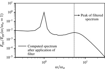
Figure 24 shows the spectrum obtained for Case C. As in Cases A and B (Rai Reference Rai2014), the computed spectrum showed slight oscillations even with a sample size of 160 shedding periods. The spectrum was filtered using a three-point filter (as in Cases A and B) to obtain a smooth curve from which the location of the second peak can be easily determined. The filtered and original spectra are nearly identical (see figure 11 in Rai Reference Rai2014 for example). Figure 24 only shows the filtered spectrum. In an effort to obtain accurate estimates of
 ${\it\omega}_{sl}/{\it\omega}_{st}$
for each of the four cases, the location of the broadband peak was obtained via a quadratic fit to the data in the region of the peak instead of using the visually observed peak. Only the data point corresponding to the observed peak and the data points to the immediate left and right of this peak were used in this process. The values of
 ${\it\omega}_{sl}/{\it\omega}_{st}$
thus obtained for cases A, B, C and D are 4.97, 2.79, 5.47 and 2.58 respectively. The estimated values for Cases A and B are slightly different from those reported in Rai (Reference Rai2014) because of the method used here to obtain
 ${\it\omega}_{sl}/{\it\omega}_{st}$
(quadratic fit), and in Case A a larger sample size (160 instead of 100 shedding periods). The difference in Case A is approximately 1.4 %, even though the sample is 60 % larger. The difference in Case B is negligible.
In addition, to test the adequacy of the sample size, the number of shedding periods over which data was collected for Case C was increased by 25 %. The frequency ratio was then computed for the baseline sample size (160 shedding periods) and
 $\pm 25\,\%$
of the baseline. The average of the three ratios was then determined. The three computed frequency ratios were found to be within
 $\pm 0.5\,\%$
of the average value. Because of the large computational costs associated with DNS, this exercise was restricted to Case C. However, the number of periods over which data were obtained for Cases A, B and D was either equal to or exceeded the baseline value for Case C.
We now assume the following power-law relationship between
 ${\it\omega}_{sl}/{\it\omega}_{st}$
and
 $\mathit{Re}_{{\it\theta}}$
and
 $\mathit{Re}_{D}$
:
 $$\begin{eqnarray}{\it\omega}_{sl}/{\it\omega}_{st}\propto \mathit{Re}_{{\it\theta}}^{{\it\alpha}}\mathit{Re}_{D}^{{\it\beta}}.\end{eqnarray}$$
The values of
 ${\it\alpha}$
and
 ${\it\beta}$
are then estimated from the data. While
 $\mathit{Re}_{D}$
is specified for each of the computations,
 $\mathit{Re}_{{\it\theta}}$
is obtained from the computations. An important question that arises is, at what location on the plate does one compute
 $\mathit{Re}_{{\it\theta}}$
? The trailing edge (
 $x/D=0.0$
) seems to be a reasonable location (the point of separation is very close to
 $x/D=0.0$
). While
 ${\it\alpha}$
and
 ${\it\beta}$
can be obtained from a least-squares fit to the data from the four cases, here we obtain these exponents from Cases A, B and C and use Case D as a validation dataset. This approach has the advantage of providing some assurance of the validity of the functional relationship (model) being used. In addition, given that the combinations of
 $\mathit{Re}_{{\it\theta}}$
and
 $\mathit{Re}_{D}$
for Cases A, B, C and D are at the vertices of a convex quadrilateral in
 $\mathit{Re}_{{\it\theta}}-\mathit{Re}_{D}$
space, prediction of
 ${\it\omega}_{sl}/{\it\omega}_{st}$
for Case D is an extrapolation, and, thus, a more severe test of the model and the exponents (than a test involving only interpolation).
The values of
 ${\it\alpha}$
and
 ${\it\beta}$
obtained are
 $-0.071$
and 0.938 respectively. The precise values may change somewhat depending on the range of
 $\mathit{Re}_{{\it\theta}}$
and
 $\mathit{Re}_{D}$
over which data are available. However, the important findings here are that (a)
 ${\it\alpha}$
is significantly smaller than
 ${\it\beta}$
in magnitude (smaller by approximately a factor of 13), so changes in
 $\mathit{Re}_{D}$
have a much greater impact on
 ${\it\omega}_{sl}/{\it\omega}_{st}$
than similar changes in
 $\mathit{Re}_{{\it\theta}}$
, (b)
 ${\it\alpha}$
is negative, thus increasing
 $\mathit{Re}_{{\it\theta}}$
at a constant value of
 $\mathit{Re}_{D}$
results in lower values of
 ${\it\omega}_{sl}/{\it\omega}_{st}$
, and (c)
 ${\it\beta}$
is close to unity (the dependence is almost linear, unlike the cylinder case where according to (3.4) the exponent is 0.67). The predicted value of
 ${\it\omega}_{sl}/{\it\omega}_{st}$
for Case D using the above values of
 ${\it\alpha}$
and
 ${\it\beta}$
in (3.5) is 2.57; the difference between the computed (2.58) and predicted values is less than 0.1 %. The prediction is accurate, thus the exponents and the model are appropriate for the range of Reynolds numbers considered here.
4. Concluding remarks
The very near and near wakes of flat plates, with turbulent separating boundary layers and vigorous shedding of vortices, are investigated with data obtained from DNS. Four different combinations of Reynolds numbers (
 $\mathit{Re}_{{\it\theta}}$
and
 $\mathit{Re}_{D}$
) have been used in the process. The emphasis here is on entrainment and the instability of the DSLs.
It was observed in Rai (Reference Rai2014) that only a small fraction of the separating turbulent boundary layer forms the DSL and participates in the initial roll-up into the shed vortex. A natural consequence of this behaviour is that for some distance downstream the wake with its shed vortices ingests fluid that was originally part of the turbulent boundary layer. The log-layer eddies are assimilated in this process and become a part of the shed vortices or the braids. A visualization of this process is provided here. A visualization of the effect of increasing
 ${\it\theta}/D$
on assimilation/entrainment is also provided; it clearly shows that wakes with larger
 ${\it\theta}/D$
values continue to assimilate boundary-layer fluid for longer (until a larger value of
 $x/D$
). The present study also shows that wake TKE profiles, in the region away from the shed vortices and braids, are very close to that of the upstream turbulent boundary layer (especially in the very near wake for the large-
 ${\it\theta}/D$
cases). This again is a consequence of the fact that much of the turbulent boundary layer does not participate in the initial shed-vortex roll-up process.
A more direct way of visualizing assimilation/entrainment in an averaged sense is proposed. We look at the distribution of the turbulent transport term in the transport equation for the phase-averaged TKE. The corresponding plot clearly shows the regions exporting turbulence and those importing turbulence. It was found that much of the transport of turbulence occurs in the braid region. The rate of turbulence transport from the shed vortices outward is noticeably smaller.
A visualization of shear-layer instability events in a (
 $t,z$
) plane showed that shear-layer vortex generation rates can vary by as much as a factor of two from event to event. Velocity fluctuations in the upstream boundary layer (for example high-speed streaks near the trailing edge) may indeed have an effect on shear-layer vortex generation rates; the data show that the high-speed streaks may result in higher rates. It remains to be seen whether there is a corresponding thinning of the shear layer or whether differences in the vortex generation rate can be attributed to changes in velocity that coincide with an instability event.
The findings of Rai (Reference Rai2014) strongly indicate that a primary cause of the shear-layer instability is the interaction between the shear layer and recirculation region vortices. This of course raises the question, do the disturbances within the shear layer (originating in the boundary layer upstream) and the log-layer eddies (that convect past the trailing edge) play a role in generating shear-layer vortices? The present study shows that log-layer eddies, like recirculation region vortices, can generate shear-layer vortices. However, because log-layer eddies are convected at a relatively high rate, they usually produce only one shear-layer vortex and continue to interact with it during their passage over the shear layer. Recirculation region vortices, on the other hand, remain in approximately the same position relative to the shear layer because of the much lower convections rates that they encounter. Thus, they tend to produce a few vortices that can be relatively powerful.
The fluctuating pressure data obtained within the DSLs clearly show a relationship between the shedding phase and shear-layer vortex generation. The intensity of the instability peaks and subsides at the vortex shedding frequency. Peak intensity within a shear layer is obtained when it is fully formed and thus maximally exposed to destabilizing agents such as recirculation region vortices.
A power-law relationship between
 ${\it\omega}_{sl}/{\it\omega}_{st}$
and
 $\mathit{Re}_{{\it\theta}}$
and
 $\mathit{Re}_{D}$
was developed based on the four cases computed. The first three cases were used to estimate the exponents and the fourth as a validation dataset. The magnitude of the exponent obtained for
 $\mathit{Re}_{{\it\theta}}$
was found to be approximately 13 times smaller than that obtained for
 $\mathit{Re}_{D}$
. Consequently, changes in
 $\mathit{Re}_{D}$
have a considerably greater effect on
 ${\it\omega}_{sl}/{\it\omega}_{st}$
than corresponding changes in
 $\mathit{Re}_{{\it\theta}}$
. The exponent associated with
 $\mathit{Re}_{{\it\theta}}$
is negative, thus an increase in
 $\mathit{Re}_{{\it\theta}}$
results in a decrease in
 ${\it\omega}_{sl}/{\it\omega}_{st}$
. Unlike the cylinder case, here we have a nearly linear relationship between
 $\mathit{Re}_{D}$
and
 ${\it\omega}_{sl}/{\it\omega}_{st}$
. The predicted value of
 ${\it\omega}_{sl}/{\it\omega}_{st}$
for Case D obtained using the power-law relation developed here was nearly the same as the computed value (in spite of the extrapolation involved), indicating that the model and the related exponents are appropriate for the range of Reynolds numbers considered here.
Acknowledgements
The contents of this paper were originally presented in the AIAA meeting paper ‘Flow features of the near wake of a flat plate with turbulent separating boundary layers’ (paper no. 2015-1967), at the AIAA 53rd Aerospace Sciences Meeting, 5–9 January 2015, Kissimmee, Florida.
Appendix A
As discussed earlier in the section on entrainment, peak normalized spanwise vorticity levels in the shed vortices (phase-averaged) at a given streamwise location decrease with increasing
 $\mathit{Re}_{{\it\theta}}$
and decreasing
 $\mathit{Re}_{D}$
. In cases where
 ${\it\theta}/D$
is significantly larger than the values considered here, shedding is expected to be much weaker and perhaps non-existent, thus resulting in thin-plate wake physics investigated in numerous studies (for example, Chevray & Kovaznay Reference Chevray and Kovaznay1969).
Clearly, it is of interest to determine the rate at which peak vorticity levels change with changing
 $\mathit{Re}_{{\it\theta}}$
and
 $\mathit{Re}_{D}$
in the case of the flat-plate wake. Here, we propose a power-law relationship very similar to the one used earlier between
 ${\it\omega}_{sl}/{\it\omega}_{st}$
and
 $\mathit{Re}_{{\it\theta}}$
and
 $\mathit{Re}_{D}$
. We assume
 $$\begin{eqnarray}{\it\Omega}_{z}\propto \mathit{Re}_{{\it\theta}}^{{\it\mu}}\mathit{Re}_{D}^{{\it\nu}},\end{eqnarray}$$
where
 ${\it\Omega}_{z}$
is the normalized phase-averaged peak spanwise vorticity at shed-vortex cores when they are located at
 $x/D=5.5$
. As before, the exponents are estimated from Cases A, B and C. Case D is used a validation dataset (validation is performed in an extrapolative mode). The exponents thus obtained are approximately
 $({\it\mu},{\it\nu})=(-0.37,0.58)$
. The estimated value of
 ${\it\Omega}_{z}$
for Case D using (A 1) is approximately 9.9 % higher in magnitude than the computed value. Although the estimate is not as accurate as that obtained for the frequency ratio, it is still quite reasonable. A linear fit to the data resulted in a substantially larger estimation error.
As discussed earlier, the ratio of peak vorticity levels for cases C, A and D (at
 $x/D=5.5$
) is 1.65:1.00:0.58. Thus,
 ${\it\Omega}_{z}$
decreases with increasing
 $\mathit{Re}_{{\it\theta}}$
and decreasing
 $\mathit{Re}_{D}$
. The computed exponents reflect this trend;
 ${\it\mu}$
is negative and
 ${\it\nu}$
is positive. The magnitude of
 ${\it\nu}$
is larger than that of
 ${\it\mu}$
. Thus, changes in
 $\mathit{Re}_{D}$
have a greater effect on
 ${\it\Omega}_{z}$
than similar changes in
 $\mathit{Re}_{{\it\theta}}$
.