1 Introduction
Quandles are nonassociative algebraic structures that are modeled on the three Reidemester moves in classical knot theory. Thus, they are appropriate algebraic structures for constructing invariants of knots and links in three-space and knotted surfaces in
 $4$
-space. Quandles were introduced independently by Joyce [Reference Joyce15] and Matveev [Reference Matveev17] in the 1980s. Quandles have been investigated in many areas of mathematics such as quasigroups and Moufang loops [Reference Elhamdadi10], the Yang–Baxter equation [Reference Carter, Elhamdadi and Saito3, Reference Ceniceros and Nelson7, Reference Ceniceros and Nelson8], representation theory [Reference Elhamdadi and Moutuou12], and ring theory [Reference Elhamdadi, Fernando and Tsvelikhovskiy11]. For more information on quandles, the reader is advised to consult the book [Reference Elhamdadi and Nelson13]. Knot theory has been extended in several directions, for example, singular knot theory. In [Reference Birman and Lin2], connections between Jones type invariants defined in [Reference Jones14] and Vassiliev invariants of singular knots defined in [Reference Vassiliev21] were established. In [Reference Juyumaya and Lambropoulou16], a variation of the Hecke algebra was used to construct a Jones-type invariant for singular knots. Combinatorial singular knot theory has the so-called generalized Reidemeister moves [Reference Juyumaya and Lambropoulou16]. These generalized moves were used in [Reference Churchill, Elhamdadi, Hajij and Nelson9] to extend the concept of quandle to an algebraic structure called singquandle to provide invariants for singular knots. In [Reference Bataineh, Elhamdadi, Hajij and Youmans1], generating sets of the generalized Reidemeister moves for oriented singular links were introduced and used to distinguish singular knots and links. In [Reference Chang and Nelson6], the quandle cocycle invariant [Reference Carter, Jelsovsky, Kamada, Langford and Saito4] was extended to oriented singular knots and used to construct a state sum invariant for singular links. Furthermore in [Reference Ceniceros, Churchill, Elhamdadi and Hajij5], the quandle polynomial invariant was extended to the case of singquandles. A singular link invariant was constructed from the singquandle polynomial and it was shown to generalize the singquandle counting invariant in [Reference Ceniceros, Churchill, Elhamdadi and Hajij5].
The article is organized as follows. In Section 2, the basics of quandle theory are reviewed, and some examples are given. Section 3 provides a review of the basic constructions of oriented singquandles as well as the singquandle counting invariant. In Section 4, we discuss the singquandle polynomial and the subsingquandle polynomial, which we introduced in a previous paper [Reference Ceniceros, Churchill, Elhamdadi and Hajij5] and used to define a singular link invariant. Section 5 defines singquandle shadows which is used to generalize the shadow colorings of knot diagrams by quandles previously defined in [Reference Ceniceros and Nelson8]. Furthermore, the shadow singquandle polynomial and the singquandle shadow polynomial invariant for a singular link L is defined. In Section 6, the shadow counting invariant is used to define an enhanced shadow link invariant by combining the shadow singquandle counting invariant and the shadow singquandle polynomial. Lastly, Section 7 examines the strength of the singquandle shadow polynomial invariant. Two examples are provided to illustrate that the singquandle shadow polynomial is sensitive to differences in singular links not detected by the singquandle coloring invariant and singquandle polynomial invariant.
2 Basics of quandles
In this paper, we consider only finite quandles and singquandles. We review the basics of quandles; more details on the topic can be found in [Reference Elhamdadi and Nelson13, Reference Joyce15, Reference Matveev17].
Definition 2.1 A set X with binary operation
 $\ast $
is called a quandle if the following three identities are satisfied.
 $$ \begin{align*} & \text{(i) } \text{For all } x \in X, x* x =x. \\ & \text{(ii) } \text{For all } y,z \in X, \text{ there is a unique } x \in X \text{ such that } x*y=z. \\ & \text{(iii) } \text{For all } x,y,z \in X, \text{ we have } (x*y)*z=(x*z)*(y*z). \end{align*} $$
From Axiom (ii) of Definition 2.1, we can write the element x as
 $z \bar {*} y = x$
. Notice that this operation
 $\bar {*}$
defines a quandle structure on X. The axioms of a quandle correspond respectively to the three Reidemeister moves of types I, II and III (see [Reference Elhamdadi and Nelson13] for examples). In fact, one of the motivations of defining quandles came from knot diagrammatic.
A quandle homomorphism between two quandles
 $(X,*)$
and
 $(Y,\triangleright )$
is a map
 $f: X \rightarrow Y$
such that
 $f(x *y)=f(x) \triangleright f(y) $
, where
 $*$
and
 $\triangleright $
denote respectively the quandle operations of X and Y. Furthermore, if f is a bijection, then it is called a quandle isomorphism between X and Y.
Some typical examples of quandles:
-
• Any nonempty set X with the operation
 $x*y=x$
, for all
$x,y \in X$
, is a quandle called a trivial quandle.
-
• Any group
$X=G$
with conjugation
$x*y=y^{-1} xy$
is a quandle. -
• Let G be an abelian group. For elements
$x,y \in G$
, define
$x*y \equiv 2y-x$
. Then
$\ast $
defines a quandle structure on G called Takasaki quandle. In case
$G=\mathbb {Z}_n$
(integers mod n) the quandle is called dihedral quandle. This quandle can be identified with the set of reflections of a regular n-gon with conjugation as the quandle operation. -
• Any
$\Lambda = (\mathbb {Z }[T^{\pm 1}])$
-module M is a quandle with
$x*y=Tx+(1-T)y$
,
$x,y \in M$
, called an Alexander quandle.


3 Oriented singquandles and the counting invariant
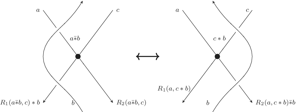
We provide a basic overview of an oriented singquandle as well as the singquandle counting invariant. For a detailed construction of oriented singquandle and the singquandle counting invariant, see [Reference Bataineh, Elhamdadi, Hajij and Youmans1, Reference Churchill, Elhamdadi, Hajij and Nelson9]. We will be adopting the following conventions at classical and singular crossings.
(a) Coloring of arcs at a positive crossing, (b) coloring of arcs at a negative crossing, and (c) colorings of semi-arcs at a singular crossing.

Generating sets of oriented singular Reidemeister moves were studied and were used to define oriented singquandles in [Reference Bataineh, Elhamdadi, Hajij and Youmans1]. We follow the naming convention for oriented singular Reidemeister moves used in [Reference Bataineh, Elhamdadi, Hajij and Youmans1]. Note that if we let
 $(S, *)$
be a quandle, we only need to consider the colorings from singular Reidemeister moves in Figures 2–4.
The Reidemeister move
 $\Omega 4a$
with colors.

The Reidemeister move
 $\Omega 4e$
with colors.

The Reidemeister move
 $\Omega 5a$
with colors.

Definition 3.1 Let
 $(X, *)$
be a quandle. Let
 $R_1$
and
 $R_2$
be two maps from
 $X \times X$
to X. The triple
 $(X, *, R_1, R_2)$
is called an oriented singquandle if the following axioms are satisfied for all
 $a,b,c \in X$
:
 $$ \begin{align} R_1(a\bar{*}b,c)*b&=R_1(a,c*b), \end{align} $$
 $$ \begin{align} \kern26ptR_2(a\bar{*}b, c) & = R_2(a,c*b)\bar{*}b, \end{align} $$
 $$ \begin{align} \kern10pt(b\bar{*}R_1(a,c))*a &= (b*R_2(a,c))\bar{*}c, \end{align} $$
 $$ \begin{align} R_2(a,b)&=R_1(b,a*b), \end{align} $$
 $$ \begin{align} \kern-41ptR_1(a,b)*R_2(a,b)&=R_2(b,a*b). \end{align} $$
Remark 3.1 We only consider oriented singquandles in this paper. Therefore, we simply refer to oriented singquandle as singquandles. For a description of unoriented singquandles, see [Reference Churchill, Elhamdadi, Hajij and Nelson9].
In [Reference Chang and Nelson6], the following family of singquandles was introduced.
Example 3.2 Let n be a positive integer, let a be an invertible element in
 $\mathbb {Z}_n$
and let
 $b,c \in \mathbb {Z}_n$
, such that
 $(1-a)(1-b-c)=0$
. Then the binary operations
 $x*y = ax+(1-a)y$
,
 $ R_1(x,y) = bx + cy$
and
 $R_2(x,y)= acx + [b+ c(1 - a)]y $
make the quadruple
 $(\mathbb {Z}_n,*, R_1,R_2)$
into an oriented singquandle.
The singquandles used in this paper are obtained from Example 3.2 with specific values of
 $a,b,$
and c.
Definition 3.2 Let
 $(X, *, R_1, R_2)$
be a singquandle. A subset
 $M \subset X$
is called a subsingquandle if
 $(M, *, R_1, R_2)$
is itself a singquandle. In particular, M is closed under the operations
 $*, R_1$
and
 $R_2$
.
We can define the notion of a homomorphism and isomorphism of oriented singquandles.
Definition 3.3 A map
 $f: X \rightarrow Y$
is called a homomorphism of oriented singquandles
 $(X, *, R_1, R_2)$
and
 $(Y, \triangleright , R^{\prime }_1, R^{\prime }_2)$
if the following conditions are satisfied for all
 $x,y \in X$
 $$ \begin{align} f(x*y)&= f(x) \triangleright f(y), \end{align} $$
 $$ \begin{align} f(R_1(x,y))&= R^{\prime}_1(f(x),f(y)), \end{align} $$
 $$ \begin{align} f(R_2(x,y))&= R^{\prime}_2(f(x),f(y)). \end{align} $$
An oriented singquandle isomorphism is a bijective oriented singquandle homomorphism. We say two oriented singquandles are isomorphic if there exists an oriented singquandle isomorphism between them.
The authors of this paper introduced the idea of a fundamental singquandle associated to a singular link L, denoted by
 $\mathcal {SQ}(L)$
, in [Reference Ceniceros, Churchill, Elhamdadi and Hajij5]. Therefore, for any oriented singular link L and an oriented singquandle
 $(S,*,R_1', R_2')$
, the set of singquandle homomorphism from
 $(\mathcal {SQ}(L),\triangleright ,R_1,R_2)$
to
 $(S, *, R_1', R_2')$
is defined by:
 $$ \begin{align*} \textrm{Hom}(\mathcal{SQ}(L),S) &= \lbrace f \, : \, \mathcal{SQ}(L) \rightarrow S \, \vert \, f( x\triangleright y) = f(x) * f(y),\\ & \quad f(R_1(x,y))= R_1'(f(x),f(y)),f(R_2(x,y))= R_2'(f(x),f(y)) \rbrace. \end{align*} $$
The set defined above was shown to be an invariant of oriented singular links in [Reference Bataineh, Elhamdadi, Hajij and Youmans1]. Furthermore, this set can be used to define computable invariants of oriented singular links. For example, by taking the cardinality of
 $\textrm {Hom}(\mathcal {SQ}(L),S)$
, we obtain the following invariant of oriented singular links.
Definition 3.4 Let L be an oriented singular link and
 $(S,*,R_1,R_2)$
be an oriented singquandles. The singquandle counting invariant is
 $$ \begin{align*} \#\textrm{Col}_S (L)=\vert \textrm{Hom}(\mathcal{SQ}(L),S) \vert. \end{align*} $$
Remark 3.3 We also note that the image,
 $\textrm {Im}(f)$
, for each
 $f \in \textrm {Hom}(\mathcal {SQ}(L),S)$
is a subsingquandle of S as shown in [Reference Ceniceros, Churchill, Elhamdadi and Hajij5].
4 Review of the singquandle polynomial
The quandle polynomial was introduced in [Reference Nelson18] and generalized in [Reference Nelson19]. In [Reference Ceniceros, Churchill, Elhamdadi and Hajij5], the authors of this paper defined the singquandle polynomial, the subsingquandle polynomial and a polynomial invariant of singular links. In this section, we give an overview of the construction of the singquandle polynomial, the subsingquandle polynomial, and the polynomial invariant of singular links. We follow the construction and notation introduced in [Reference Ceniceros, Churchill, Elhamdadi and Hajij5].
Definition 4.1 Let
 $(X,*,R_1,R_2)$
be a finite singquandle. For every
 $x \in X$
, define
 $$ \begin{align*} C^1(x) = \lbrace y \in X \, \vert \, y * x = y \rbrace \quad \text{and} \quad R^1(x) = \lbrace y \in X \, \vert \, x * y = x \rbrace, \end{align*} $$
 $$ \begin{align*} C^2(x) = \lbrace y \in X \, \vert \, R_1(y , x) = y \rbrace \quad \text{and} \quad R^2(x) = \lbrace y \in X \, \vert \, R_1(x , y) = x \rbrace, \end{align*} $$
 $$ \begin{align*} C^3(x) = \lbrace y \in X \, \vert \, R_2(y , x) = y \rbrace \quad \text{and} \quad R^3(x) = \lbrace y \in X \, \vert \, R_2(x , y) = x \rbrace. \end{align*} $$
Let
 $c^i(x) = \vert C^i(x)\vert $
and
 $r^i(x) = \vert R^i(x)\vert $
for
 $i=1,2,3$
. Then the singquandle polynomial of X is
 $$ \begin{align*} sqp(X) = \sum_{x\in X} s_1^{r^1(x)}t_1^{c^1(x)}s_2^{r^2(x)}t_2^{c^2(x)}s_3^{r^3(x)}t_3^{c^3(x)}. \end{align*} $$
We note that the value
 $r^i(x)$
is the number of elements in X that act trivially on x, while
 $c^i(x)$
is the number of elements of X on which x acts trivially via
 $*, R_1$
and
 $R_2.$
Furthermore, if
 $Y \subset X$
is a subsingquandle we can define the following singquandle polynomial for Y as a subsignquandle of X.
Definition 4.2 Let
 $(X,*, R_1,R_2)$
be a finite singquandle and
 $S \subset X$
a subsingquandle. Then the subsingquandle polynomial is
 $$ \begin{align*} Ssqp(S \subset X ) = \sum_{x \in S} s_1^{r^1(x)}t_1^{c^1(x)}s_2^{r^2(x)}t_2^{c^2(x)}s_3^{r^3(x)}t_3^{c^3(x)}. \end{align*} $$
The subsingquandle polynomials can be thought of as the contributions to the singquandle polynomial coming from the subsingquandles we are considering. Using the subsingquandles polynomial we can now define the following polynomial invariant of singular links.
Definition 4.3 Let L be a singular link,
 $(X,*,R_1,R_2)$
a finite singquandle. Then the multiset
 $$ \begin{align*} \Phi_{Ssqp}(L,X) = \lbrace Ssqp(Im(f) \subset X) \, \vert \, f \in \text{Hom}(\mathcal{SQ}(L), X\rbrace \end{align*} $$
is the subsingquandle polynomial invariant of L with respect to X. We can also represent this invariant in the following polynomial-style form by converting the multiset elements to exponents of a formal variable u and converting their multiplicities to coefficients:
 $$ \begin{align*} \phi_{Ssqp}(L,X) = \sum_{f \in \textrm{Hom}(\mathcal{SQ}(L),X)} u^{Ssqp(Im(f) \subset X)}. \end{align*} $$
Example 4.1 Consider the two-bouquet graphs of type L listed as
 $1^l_1$
in [Reference Oyamaguchi20]. Let
 $(S,*,R_1,R_2)$
be the singquandle with
 $S=\mathbb {Z}_4$
and operations
 $x*y = 3x-2y = x\bar {*}y$
,
 $R_1(x,y)=2 x + 3 y$
, and
 $R_2(x,y)=x$
.
Diagram of
 $1_1^l$
.

We can identify each coloring of
 $1_1^l$
by S with the triple
 $(f(x),f(y),f(z))$
. Using the fact that
 $z = R_1(x,y), x = R_2(x,y)$
and
 $z * x =y,$
by a straightforward computation we obtain the following colorings:
 $$ \begin{align*} &\textrm{Hom}(\mathcal{SQ}(1_1^l),S)\\ &\quad = \{(1, 1, 1), (1, 2, 0), (1, 3, 3), (1, 0, 2), (2, 1, 3), (2, 2, 2), (2, 3, 1), (2, 0, 0),\\ &\quad\qquad (3, 1, 1), (3, 2, 0), (3, 3, 3), (3, 0, 2), (0, 1, 3), (0, 2, 2), (0, 3, 1), (0, 0, 0)\}. \end{align*} $$
Therefore,
 $\#\textrm {Col}_S (1_1^l)=16$
. We compute
 $r^i$
and
 $c^i$
for
 $i=1,2,3$
:
 $$ \begin{align*} \begin{array}{ r| c c } x & r^1(x) & c^1(x) \\ \hline 1& 2 & 2 \\ 2& 2 & 2 \\ 3& 2 & 2 \\ 0& 2 & 2 \\ \end{array} \qquad \begin{array}{ r| c c } x & r^2(x) & c^2(x)\\ \hline 1& 1 & 1 \\ 2& 1 & 1 \\ 3& 1 & 1 \\ 0& 1 & 1 \\ \end{array} \qquad \begin{array}{ r| c c } x &r^3(x) &c^3(x) \\ \hline 1& 4& 4\\ 2& 4 & 4 \\ 3& 4 & 4 \\ 0& 4 & 4 \\ \end{array}. \end{align*} $$
In order to compute the subsingquandle polynomial invariant of
 $1_1^l$
, we consider the corresponding subsingquandle for each coloring. Therefore, we obtain
 $$ \begin{align*} \phi_{Ssqp}(1_1^l,S) = 4 u^{s_1^2 t_1^2 s_2 t_2 s_3^4 t_3^4}+4 u^{2 s_1^2 t_1^2 s_2 t_2 s_3^4 t_3^4}+8 u^{4 s_1^2 t_1^2 s_2 t_2 s_3^4 t_3^4}. \end{align*} $$
5 Singquandle shadows
In this section, we define singquandle shadows which can be used to generalize the shadow colorings of knot diagrams by quandles previously defined in [Reference Ceniceros and Nelson8].
Definition 5.1 Let
 $(S,*,R_1,R_2)$
be a singquandle. An S-set is a set X and a map
 $\cdot : X \times S \rightarrow X$
satisfying the following conditions:
-
1 For all
$s \in S$
,
$\cdot s : X \rightarrow X$
mapping x to
$x \cdot s$
is a bijection.


The meaning of these two equations will become clear from Figure 7.
Definition 5.2 A singquandle shadow or S-shadow is the pair of an oriented sinquandle
 $(S,*,R_1,R_2)$
and a S-set
 $(X,\cdot )$
, denoted by
 $(S,X,*,R_1,R_2,\cdot )$
or simply by
 $(S,X)$
. Let
 $S^{\prime }$
be a subsingquandle of S. A subset Y of X closed under the action of
 $S^{\prime }$
is an subshadow of
 $(S,X)$
, which we denote by
 $(S^\prime , Y) \subset (S,X)$
.
The following definition will allow us to present a shadow operation in an alternate form that will be useful in later sections.
Definition 5.3 When
 $(X,S)$
is a singquandle shadow with X and S finite, the shadow matrix of the singquandle shadow
 $(X = \lbrace x_1, \dots , x_m \rbrace $
,
 $S = \lbrace s_1,\dots , s_n \rbrace )$
is the
 $m \times n$
matrix whose
 $(i,j)$
entry is k where
 $x_k = x_i \cdot s_j$
.
Let
 $(S,*,R_1,R_2)$
and
 $(S',\triangleright , R^{\prime }_1,R^{\prime }_2)$
be singquandles. Furthermore, let
 $(X, \cdot )$
be an S-set and
 $(X', \bullet )$
be an
 $S'$
-set. A map
 $f: S \rightarrow S'$
makes
 $X'$
inherit a natural action of S via the map f by
 $x' \cdot s :=x' \bullet f(s)$
.
Definition 5.4 A homomorphism of sinquandle shadows between
 $(S,X,*,R_1,R_2,\cdot )$
and
 $(S',Y,\triangleright ,R^{\prime }_1,R^{\prime }_2,\bullet )$
is a pair of maps
 $\phi :(X, \cdot ) \rightarrow (Y,\bullet )$
and
 $f:(S,*,R_1,R_2) \rightarrow (S',\triangleright ,R^{\prime }_1,R^{\prime }_2)$
, such that f is a singquandle homomorphism, that is the identities (3.6)–(3.8) are satisfied and for all
 $x \in X$
and
 $s \in S$
, we have
 $$ \begin{align} \phi(x \cdot s)=\phi(x) \bullet f(s). \end{align} $$
Furthermore, if
 $\phi $
and f are bijections then we have a singquandle shadow isomorphism.
From this definition, it is straightforward to obtain the following lemma.
Lemma 5.1
 $(Im(f),Im(\phi ),\triangleright ,R^{\prime }_1,R^{\prime }_2,\bullet )$
is a subshadow of
 $(S',Y,\triangleright ,R^{\prime }_1,R^{\prime }_2,\bullet )$
.
Example 5.2 Let
 $(S,*,R_1,R_2)$
be an oriented singquandle with
 $S=\mathbb {Z}_8=\{ 1,2,3,4,5,6,7,0 \}$
,
 $x*y = 5x-4y = x\bar {*}y$
,
 $R_1(x,y) =3x+4y $
, and
 $R_2(x,y)= 4x+3y$
. Then the four element set
 $X= \mathbb {Z}_4=\{ 1,2,3,0 \}$
with map
 $\cdot s : \mathbb {Z}_4 \rightarrow \mathbb {Z}_4$
for each
 $s \in S$
defined by
 $x\cdot s = x + 2 s + s^2$
is a singquandle shadow. Note that
 $\cdot $
has the following operation table
 $$ \begin{align*} \begin{array}{r|cccccccc} \cdot & 1 & 2 & 3 & 4 & 5 & 6 & 7 & 0\\ \hline 1& 0 & 1 & 0 & 1 & 0 & 1 & 0 & 1 \\ 2& 1 & 2 & 1 & 2 & 1 & 2 & 1 & 2 \\ 3& 2 & 3 & 2 & 3 & 2 & 3 & 2 & 3 \\ 0& 3 & 0 & 3 & 0 & 3 & 0 & 3 & 0 \\ \end{array} \end{align*} $$
Furthermore, by Definition 5.3, the shadow operation
 $\cdot $
can be presented by the shadow matrix,
 $$ \begin{align*} \left[ \begin{array}{cccccccc} 0 & 1 & 0 & 1 & 0 & 1 & 0 & 1 \\ 1 & 2 & 1 & 2 & 1 & 2 & 1 & 2 \\ 2 & 3 & 2 & 3 & 2 & 3 & 2 & 3 \\ 3 & 0 & 3 & 0 & 3 & 0 & 3 & 0 \\ \end{array} \right]. \end{align*} $$
Example 5.3 Let
 $(S,*,R_1,R_2)$
be any oriented singquandle and let
 $X = S$
. Then X is a singquandle shadow under the shadow operation
 $x \cdot s = x * s$
for all
 $x,y \in S$
, since we have
 $$ \begin{align} (x \cdot s_1) \cdot s_2 &= (x * s_1)*s_2 \nonumber\\ &= (x * s_2) * (s_1 * s_2) \nonumber\\ &= (x\cdot s_2) \cdot (s_1 \cdot s_2), \end{align} $$
and
 $$ \begin{align} (x \cdot s_1) \cdot s_2 &= (x * s_1)*s_2 \nonumber\\ &= (x * R_1 (s_1,s_2)) * R_2(s_1,s_2) \nonumber\\ &= (x \cdot R_1 (s_1,s_2)) \cdot R_2(s_1,s_2). \end{align} $$
Remark 5.4 Equation (5.2) is satisfied by the self-distributitive property of
 $*$
. On the other hand, equation (5.3) is satisfied by applying a combination of singquandle properties. Consider equation (3.3) in the definition of a singquandle, let
 $b = c$
. Therefore, we obtain
 $$ \begin{align*} (c \bar{*} R_1(a,c))* a = (c * R_2(a,c)) \bar{*} c, \end{align*} $$
which can be written as
 $$ \begin{align*} ((c \bar{*} R_1(a,c))* a)*c = c * R_2(a,c). \end{align*} $$
Now, we let
 $w = c \bar {*} R_1(a,c) \iff w * R_1(a,c) = c$
. Next, we make the appropriate substitution to obtain
 $$ \begin{align*} (w *a) * c = (w * R_1(a,c)) * R_2(a,c). \end{align*} $$
Lastly, let
 $w=x$
,
 $a = s_1$
, and
 $b = s_2$
to obtain
 $$ \begin{align*} (x * s_1)*s_2 = (x * R_1 (s_1,s_2)) * R_2(s_1,s_2). \end{align*} $$
Let D be a diagram of an oriented singular link L. We denoted the set of arcs of D by
 $\mathcal {A}(D)$
and the connected regions of
 $\mathbb {R}^2\setminus D$
by
 $\mathcal {R}(D)$
. Using the notion of a singquandle homomorphism given in Definition 3.3, we have the following notion of colorings by singquandles.
Definition 5.5 Let
 $(S,*, R_1, R_2)$
be an oriented singquandle. An S-coloring of D is a map
 $f: \mathcal {A}(D) \rightarrow S$
such that at a crossing with
 $u_1, u_2, o_1 \in \mathcal {A}(D)$
and at a singular crossing with
 $a_1,a_2,a_3,a_4 \in \mathcal {A}(D)$
the following conditions are satisfied,
 $$ \begin{align} f(u_2) = f(u_1) * f(o_1), \end{align} $$
 $$ \begin{align} f(a_3) = R_1(f(a_1),f(a_2)), \end{align} $$
 $$ \begin{align} f(a_4) = R_2(f(a_1),f(a_2)). \end{align} $$
The conditions above are illustrated in Figure 6.
Arcs and regions of diagram D.

Shadow coloring at positive, negative, and singular crossings.

Definition 5.6 Let
 $(S,X,*, R_1, R_2, \cdot )$
be a shadow singquandle. An
 $(S,X)$
-coloring of D is a map
 $f \times \phi : \mathcal {A}(D) \times \mathcal {R}(D) \rightarrow S \times X$
satisfying the following conditions,
-
• f is an S-coloring of D.
-
•
$\phi (\mathcal {R}(D)) \subset X$
. -
• For
$a \in \mathcal {A}(D)$
and
$x_1, x_2 \in \mathcal {R}(D)$
the following (5.7)
$$ \begin{align} \phi(x_1) \cdot f(a) = \phi(x_2). \end{align} $$


The condition above is illustrated in Figure 6.
When there is no confusion, we refer to an
 $(S,X)$
-coloring by a shadow coloring of D.
We denote a region coloring by a box around the shadow element and denote an arc coloring by an element of a singquandle without a box. Note that the conditions required for the set X to be an S-set for some oriented sinquandle are the conditions needed to guarantee that shadow colorings are well defined at crossings, see Figure 7.
Proposition 5.5 Let L be a singular link diagram and
 $(S,X,*,R_1,R_2,\cdot )$
be a singquandle shadow. Then for each singquandle coloring of L by S and each element of X there is exactly one shadow coloring of L.
Proof. Consider a singquandle coloring of L and choose a region of L. Any element of X can be assigned to the chosen region, and any choice determines a unique shadow color of each region by following the rule in Figure 6.▪
Definition 5.7 Let L be singular link diagram and
 $(S,X)$
is a singquandle shadow. The shadow counting invariant,
 $\#\textrm {Col}_{(S,X)}(L)$
, is the number of shadow colorings of L by
 $(S,X)$
.
Example 5.6 Let
 $(S,*,R_1,R_2)$
be the singquandle with
 $S=\mathbb {Z}_{10}$
and operations defined by
 $x*y = x= x \bar {*} y $
,
 $R_1(x,y) = 4x$
, and
 $R_2(x,y) = 4y$
. We can define a shadow structure by
 $X=\mathbb {Z}_4$
with the map
 $\cdot s: \mathbb {Z}_4 \rightarrow \mathbb {Z}_4$
for each
 $s \in S$
defined by
 $x\cdot s= 3 x + 2 s + 2 s^2$
. We also represent this shadow operation by the shadow matrix
 $$ \begin{align*} \left[ \begin{array}{cccccccccc} 3 & 3 & 3 & 3 & 3 & 3 & 3 & 3 & 3 & 3 \\ 2 & 2 & 2 & 2 & 2 & 2 & 2 & 2 & 2 & 2 \\ 1 & 1 & 1 & 1 & 1 & 1 & 1 & 1 & 1 & 1 \\ 0 & 0 & 0 & 0 & 0 & 0 & 0 & 0 & 0 & 0 \\ \end{array} \right]. \end{align*} $$
We compute a shadow coloring for the following two-bouquet graph of type K listed as
 $3_1^k$
in [Reference Oyamaguchi20]. This singular knot has one coloring by S given by
 $$ \begin{align*}\textrm{Hom}(\mathcal{SQ}(3_1^k),S) =\lbrace (s_1\to 0,s_2 \to 0, s_3 \to 0, s_4 \to 0)\rbrace. \end{align*} $$
For this coloring, we also obtain one shadow coloring for each element of X. Therefore, we have the following four shadow colorings by the above shadow singquandle.
Shadow coloring of
 $3_1^k$
.

Shadow colorings of
 $3_1^k$
by singquandle shadow X.

Therefore,
 $\#\textrm {Col}_{(S,X)}(3_1^k) = 4.$
The following corollary implies that the shadow counting invariant does not contain any information not contained by the singquandle counting invariant. We obtain the following result by noticing that for each coloring of an oriented singular link by an oriented singquandle, we have a different shadow coloring for each element in the S-set.
Corollary 5.7 The shadow counting invariant of a singular link L by the S-shadow
 $(S,X)$
is given by
 $$ \begin{align*}\# \textrm{Col}_{(S,X)}(L) = \vert X \vert \, \# \textrm{Col}_S(L) ,\end{align*} $$
where
 $\#\textrm {Col}_S(L)$
is the singquandle counting invariant.
We can define the following polynomial for a sinquandle shadow to obtain a singquandle shadow invariant.
Definition 5.8 The shadow singquandle polynomial, denoted by
 $\textrm {sp}(S,X)$
, of the shadow singquandle
 $(S,X,*,R_1,R_2,\cdot )$
is the sum
 $$ \begin{align*} \textrm{sp}(S,X) = \sum_{x \in X} t^{r(x)}, \end{align*} $$
where
 $r(x) = \vert \lbrace s \in S \,; \, x \cdot s = x \rbrace \vert $
. Furthermore, If
 $(S^{\prime },Y)$
is a subshadow of
 $(S,X)$
, then the subshadow singquandle polynomial of
 $(S^{\prime },Y)$
is
 $$ \begin{align*} \textrm{Subsp} ((S',Y) \subset (S,X)) = \sum_{x \in Y} t^{r(x)}, \end{align*} $$
where
 $r(x) =\vert \lbrace s' \in S' \,; \, x \cdot s' = x \rbrace \vert $
.
Example 5.8 Let
 $S= \mathbb {Z}_6 =\{ 1,2,3,4,5,0\}$
with singquandle operations defined by
 $x* y = 5x-4y = x\bar {*}y$
,
 $R_1(x,y)=3x+4y$
and
 $R_2(x,y)= 2x+5y$
. We can define a shadow structure by
 $X = \mathbb {Z}_2 = \{1,0\}$
with the map
 $\bullet s: \mathbb {Z}_2 \rightarrow \mathbb {Z}_2$
for each
 $s \in S$
defined by
 $x\bullet s= x$
. We can also represent the shadow operation with the shadow matrix
 $$ \begin{align*} \left[ \begin{array}{cccccc} 1 & 1 & 1 & 1 & 1 & 1 \\ 0 & 0 & 0 & 0 & 0 & 0 \\ \end{array} \right]. \end{align*} $$
Note that we can compute
 $r(x)$
for each
 $x \in X$
by going through the row of the shadow matrix and counting the occurrences of the row number. Therefore,
 $r(1)=6$
and
 $r(0) = 6$
, and the shadow singquandle polynomial of
 $(S,X)$
is
 $$ \begin{align*} \textrm{sp}(S,X) = 2t^6. \end{align*} $$
We consider two types of subshadows. We first consider a subset of X closed under the action of S. When we consider the subshadow
 $(S, Y) \subset (S,X)$
, where
 $Y = \{1\}$
, note that we can check from the shadow matrix that Y is closed under the action of S. The subshadow
 $(S,Y)$
has the following subshadow singquandle polynomial
 $$ \begin{align*} \textrm{Subsp}(S,Y) = t^6. \end{align*} $$
Next, we consider the subshadow
 $(S',Y) \subset (S,X)$
, where
 $S'$
is the subsingquandle consisting of
 $\{2,4,0\}$
and
 $Y = \{1 \}$
. A straightforward computation shows that
 $S^\prime $
is closed under the singquandle operations. Furthermore, we check from the shadow matrix that Y is closed under the action of
 $S^\prime $
. The subshadow
 $(S',Y)$
has the following subshadow singquandle polynomial,
 $$ \begin{align*} \textrm{Subsp}(S^\prime,Y)= t^3. \end{align*} $$
We now prove that the shadow singquandle polynomial is an invariant of shadow singquandles.
Proposition 5.9 Let
 $(S,X)$
and
 $(S',Y)$
be two singquandle shadows. If
 $(S,X)$
and
 $(S',Y)$
are isomorphic, then they have equal shadow polynomials,
 $\textrm {sp}(S,X) = \textrm {sp}(S',Y)$
.
Proof. Suppose the pair
 $\phi : X \rightarrow Y$
and
 $f: S \rightarrow S'$
is a shadow singquandle isomorphism. Then
 $r(\phi (x)) = r(x)$
and the contribution to
 $\textrm {sp}(S,X)$
from
 $x \in X$
is the same as the contribution of
 $\phi (x) \in Y$
to
 $\textrm {sp}(S',Y)$
. Since
 $\phi $
and f are bijective maps satisfying equations (3.6)–(5.1), the result follows.▪
The shadow polynomial can be used to distinguish and classify shadow singquandles. In the following example, we distinguish two shadow singquandles.
Example 5.10 Let
 $(S,*,R_1,R_2)$
be a singquandle, as in Example 5.2, with
 $S= \mathbb {Z}_8$
,
 $x*y= 5x-4y = x \bar {*} y$
,
 $R_1(x,y) = 3 x + 4 y$
, and
 $R_2(x,y)= 4x+3y$
. We can define a shadow structure by
 $X=\mathbb {Z}_4$
with the map
 $\cdot s: \mathbb {Z}_4 \rightarrow \mathbb {Z}_4$
for each
 $s \in S$
defined by
 $x\cdot s= x + 2 s + s^2$
. We also represent this shadow operation by the shadow matrix
 $$ \begin{align*} \left[ \begin{array}{cccccccc} 0 & 1 & 0 & 1 & 0 & 1 & 0 & 1 \\ 1 & 2 & 1 & 2 & 1 & 2 & 1 & 2 \\ 2 & 3 & 2 & 3 & 2 & 3 & 2 & 3 \\ 3 & 0 & 3 & 0 & 3 & 0 & 3 & 0 \\ \end{array} \right]. \end{align*} $$
The
 $(S,X, *, R_1,R_2,\cdot )$
is a singquandle shadow with shadow polynomial
 $$ \begin{align*} \textrm{sp}(S,X) = 4t^4. \end{align*} $$
Let
 $W = \mathbb {Z}_4$
. We can define a shadow structure by
 $X=\mathbb {Z}_4$
with the map
 $\bullet s: \mathbb {Z}_4 \rightarrow \mathbb {Z}_4$
for each
 $s \in S$
defined by
 $x\bullet s= 3 x + 2 s + 2 s^2$
. We can also represent the shadow operation with the shadow matrix
 $$ \begin{align*} \left[ \begin{array}{cccccccc} 3 & 3 & 3 & 3 & 3 & 3 & 3 & 3 \\ 2 & 2 & 2 & 2 & 2 & 2 & 2 & 2 \\ 1 & 1 & 1 & 1 & 1 & 1 & 1 & 1 \\ 0 & 0 & 0 & 0 & 0 & 0 & 0 & 0 \\ \end{array} \right]. \end{align*} $$
The
 $(S,W, *, R_1,R_2,\bullet )$
is a singquandle shadow with shadow polynomial
 $$ \begin{align*} \textrm{sp}(S,W) = 2+2t^8. \end{align*} $$
We see that the shadow singquandle polynomial is an effective invariant of singquandle shadows.
In this section, we see that by simply computing the shadow counting invariant of an oriented singular link, we do not obtain any more information than that obtained from the singquandle counting invariant. Therefore, in the following section, we enhance the shadow counting invariant in order to obtain a stronger invariant.
6 Enhanced shadow counting invariant
In this section, we jazz up the shadow counting invariant from the previous section. We combine the S-shadow counting invariant and the shadow polynomial in order to define an enhanced shadow singquandle invariant for singular link.
Definition 6.1 Let
 $f \times \phi $
be a shadow coloring of an oriented singular link diagram D. The closure of the set of shadow colors under the action of the image subsingquandle
 $\textrm {Im}(f) \subset S$
of
 $f \times \phi $
is a subshadow called the shadow image of
 $f \times \phi $
, which we denote by
 $\textrm {om}(f \times \phi )$
.Footnote
1
Definition 6.2 Let
 $(S,X)$
be an S-shadow and let L be an oriented singular link with diagram D. The singquandle shadow polynomial invariant of L with respect
 $(S,X)$
is
 $$ \begin{align*} SP(L) = \sum_{f \times \phi \in \mbox{shadow coloring}} u^{\textrm{Subsp} (\textrm{om}(f \times \phi) \subset (S,X))}.\end{align*} $$
7 Examples
In this section, we present two examples in which we show that the shadow sinquandle polynomial is an enhancement of the singquandle counting invariant. In the first example, we include a pair of singular knots with the same singquandle counting invariant and the same singquandle polynomial but are distinguished by the singquandle shadow polynomial invariant. The computations were performed by Mathematica and python independently and checked by hand.
Example 7.1 Let
 $(S,X,*,R_1,R_2,\cdot )$
be the shadow singquandle with
 $S=\mathbb {Z}_8$
,
 $X=\mathbb {Z}_6$
and operations
 $x*y = 3x-2y = x \bar {*} y$
,
 $R_1(x,y) = 7x+6y$
,
 $R_2(x,y) = 2x+3y$
, with map
 $\cdot s: \mathbb {Z}_6 \rightarrow \mathbb {Z}_6$
for each
 $s \in S$
defined by
 $x\cdot s= x + 3 s$
. We can also represent the shadow structure by the shadow matrix
 $$ \begin{align*} \left[ \begin{array}{cccccccc} 4 & 1 & 4 & 1 & 4 & 1 & 4 & 1 \\ 5 & 2 & 5 & 2 & 5 & 2 & 5 & 2 \\ 0 & 3 & 0 & 3 & 0 & 3 & 0 & 3 \\ 1 & 4 & 1 & 4 & 1 & 4 & 1 & 4 \\ 2 & 5 & 2 & 5 & 2 & 5 & 2 & 5 \\ 3 & 0 & 3 & 0 & 3 & 0 & 3 & 0 \\ \end{array} \right]. \end{align*} $$
The following two two-bouquet graph of type K listed as
 $4_1^k$
and
 $5_4^k$
in [Reference Oyamaguchi20]. We obtain the following coloring equations from the singular knot
 $4_1^k$
,
 $$ \begin{align*} s_1 &= s_6 \bar{*} s_2 =-2 s_2 + 3 s_6, \\ s_2 &= s_5 \bar{*} s_6 = 3 s_5 - 2 s_6, \\ s_3 &= R_1(s_1,s_2) = 7 s_1 + 6 s_2, \\ s_4 &= R_2(s_1,s_2) =2 s_1 + 3 s_2, \\ s_5 &= s_4 \bar{*}s_3 =-2 s_3 + 3 s_4, \\ s_6 &= s_3 \bar{*} s_5 = 3 s_3 - 2 s_5. \end{align*} $$
From these equations, we obtain the colorings listed below. In the following list we identify each coloring
 $f \in \textrm {Hom}(\mathcal {SQ}(4_1^k),S)$
with the six-tuple
 $(f(s_1),f(s_2),f(s_3),f(s_4),f(s_5),f(s_6))$
.
 $$ \begin{align*} &\textrm{Hom}(\mathcal{SQ}(4_1^k),S)\\ &\quad= \{(1, 7, 1, 7, 3, 5), (1, 3, 1, 3, 7, 5), (2, 2, 2, 2, 2, 2), (2, 6, 2, 6, 6, 2), \\ &\qquad\quad(3, 5, 3, 5, 1, 7), (3, 1, 3, 1, 5, 7), (4, 0, 4, 0, 0, 4),(4, 4, 4, 4, 4, 4), \\ &\qquad\quad(5, 3, 5, 3, 7, 1), (5, 7, 5, 7, 3, 1), (6, 6, 6, 6, 6, 6), (6, 2, 6, 2, 2, 6), \\ &\qquad\quad(7, 1, 7, 1, 5, 3), (7, 5, 7, 5, 1,3), (0, 4, 0, 4, 4, 0), (0, 0, 0, 0, 0, 0)\}. \end{align*} $$
We obtain the following coloring equations from the singular knot
 $5_4^k$
,
 $$ \begin{align*} s_1 &= s_7 \bar{*} s_5 = -2 s_5 + 3 s_7,\\ s_2 &= s_4 * s_6 = 3 s_4 - 2 s_6,\\ s_3 &= R_1(s_1,s_2) = 7 s_1 + 6 s_2, \\ s_4 &= R_2(s_1,s_2) =2 s_1 + 3 s_2, \\ s_5 &= s_3 \bar{*}s_7 = 3 s_3 - 2 s_7, \\ s_6 &= s_5 * s_2 = 2 s_2 + 3 s_5,\\ s_7 &= s_6 \bar{*}s_3 =-2 s_3 + 3 s_6. \end{align*} $$
From these equations, we obtain the colorings listed below. In the following list, we identify each coloring
 $f \in \textrm {Hom}(\mathcal {SQ}(5_4^k),S)$
with the six-tuple
 $(f(s_1),f(s_2),f(s_3), f(s_4),f(s_5),f(s_6))$
.
 $$ \begin{align*} &\textrm{Hom}(\mathcal{SQ}(5_4^k),S)\\ &\quad=\{(2, 2, 2, 2, 2, 2, 2), (2, 4, 6, 0, 6, 2, 2), (2, 6, 2, 6, 2, 2, 2), (2, 0, 6, 4, 6, 2, 2), \\ &\qquad\quad(4, 2, 0, 6, 0, 4, 4), (4, 4, 4, 4, 4, 4, 4), (4, 6, 0, 2, 0, 4, 4), (4, 0, 4, 0, 4, 4, 4), \\ &\qquad\quad(6, 2, 6, 2, 6, 6, 6), (6, 4, 2, 0, 2, 6, 6), (6, 6, 6, 6, 6, 6, 6), (6, 0, 2, 4, 2, 6, 6), \\ &\qquad\quad(0, 2, 4, 6, 4, 0, 0), (0, 4, 0, 4, 0, 0, 0), (0, 6, 4, 2, 4, 0, 0), (0, 0, 0, 0, 0, 0, 0) \}. \end{align*} $$
Therefore, both singular knots have the same singquandle counting invariant
 $\#\textrm {Col}_S(4_1^k) = 16 = \#\textrm {Col}_S(5_4^k)$
. Therefore, by Theorem 5.7, we obtain that the two singular knots have the same shadow counting invariant
 $\#\textrm {Col}_{(S,X)}(4_1^k) = 96 = \#\textrm {Col}_{(S,X)}(5_4^k)$
. Furthermore, the two singular knots have the same singquandle polynomial
 $\phi _{Ssqp}(4_1^k)=4 u^{s_1^2 t_1^2 s_2^2 t_2^2 s_3 t_3}+4 u^{2 s_1^2 t_1^2 s_2^2 t_2^2 s_3 t_3}+8 u^{4 s_1^2 t_1^2 s_2^2 t_2^2 s_3 t_3} =\phi _{Ssqp}(5_4^k) $
. However, the singquandle shadow polynomial invariant distinguishes the two singular knots:
Singular knots
 $4_1^k$
and
 $5_4^k$
and corresponding
 $SP$
invariant.

Example 7.2 Let
 $(S,X,*,R_1,R_2,\cdot )$
with
 $S=\mathbb {Z}_{12}$
,
 $X=\mathbb {Z}_8$
,
 $x*y = 11x-10y = x \bar {*} y$
,
 $R_1(x,y) = x+6y$
,
 $R_2(x,y) = 6x+y$
, with map
 $\cdot s: \mathbb {Z}_8 \rightarrow \mathbb {Z}_8$
for each
 $s \in S$
defined by
 $x\cdot s= x + 6 s + 3 s^2 + 2 s^3$
. We can also represent the shadow structure by the shadow matrix
 $$ \begin{align*} \left[ \begin{array}{cccccccccccc} 4 & 1 & 4 & 1 & 4 & 1 & 4 & 1 & 4 & 1 & 4 & 1 \\ 5 & 2 & 5 & 2 & 5 & 2 & 5 & 2 & 5 & 2 & 5 & 2 \\ 6 & 3 & 6 & 3 & 6 & 3 & 6 & 3 & 6 & 3 & 6 & 3 \\ 7 & 4 & 7 & 4 & 7 & 4 & 7 & 4 & 7 & 4 & 7 & 4 \\ 0 & 5 & 0 & 5 & 0 & 5 & 0 & 5 & 0 & 5 & 0 & 5 \\ 1 & 6 & 1 & 6 & 1 & 6 & 1 & 6 & 1 & 6 & 1 & 6 \\ 2 & 7 & 2 & 7 & 2 & 7 & 2 & 7 & 2 & 7 & 2 & 7 \\ 3 & 0 & 3 & 0 & 3 & 0 & 3 & 0 & 3 & 0 & 3 & 0 \\ \end{array} \right]. \end{align*} $$
We compute the shadow polynomial for the singular knots in Figure 11 derived from the classical trefoil knot.
Colorings of the singular knots derived from the trefoil.


In this example, we have a collection of singular knots that can be distinguished by a combination of the counting invariant and the shadow singquandle polynomial invariant. We see that the counting invariant distinguishes
 $K_3$
from
 $K_2$
and
 $K_1$
. Furthermore,
 $K_2$
and
 $K_1$
are distinguished by their shadow singquandle polynomial.
Acknowledgment
The authors of this paper thank the referee for all the fruitful comments and pointing out an error in our Mathematica code. The authors also thank Sam Nelson for fruitful discussion and Hamza Elhamdadi for providing python code to verify the examples in Section 7.