Nomenclature
-
 $a$
-
avoidance maneuvers executed by the UAV
-
$d_{i}$
-
distance from the UAV to the i-th obstacle
-
$h_{i}$
-
the vertical projection of the intrusion distance of the i-th obstacle
-
$L$
-
length of UAV Flight Path
-
$N_{D}$
-
the number of detection sectors
-
$o^{k,n}$
-
observation information of the designated sector block by the UAV
-
$P_{goal}$
-
the positional coordinates of the target
-
$R^{D}$
-
detection radius of the UAV
-
$R^{H}$
-
detection altitude of the UAV
-
$t$
-
discrete time steps
- UAV
-
unmanned aerial vehicle
-
$z$
-
the altitude of the UAV


Greek symbol
-
$\varphi$
-
the climb angle of the UAV
-
$\phi$
-
the azimuth angle of the UAV


1.0 Introduction
With rapid advances in autonomous navigation and deep learning technologies, unmanned aeriel vehicles (UAVs) have become essential tools across multiple domains including logistics, agricultural monitoring and search-and-rescue operations [Reference Guebsi1, Reference Jahani2]. Their compact size, lightweight design, cost-effectiveness and high manoeuverability make them particularly suitable for these applications. However, these operational environments often contain unpredictable dynamic obstacles. Collisions may damage or destroy UAVs, leading to economic losses and potential safety hazards. Ensuring safe UAV operations is therefore a primary engineering concern, with autonomous obstacle avoidance in complex environments being critical for operational safety.
Current UAV operations are predominantly conducted in segregated airspace and typically rely on offline global planning to generate deconflicted trajectories, with takeoff and landing executed according to a preplanned route. To accommodate environmental changes and model uncertainties, research has progressively expanded to local replanning, whereby the en-route path is updated from recent observations to improve feasibility without altering the overall mission objective. With the rapid growth of low-altitude applications, research on autonomous obstacle avoidance has become essential to enable safe and scalable UAV operations in complex urban environments. Existing studies and pilot deployments have pushed simulation settings toward more realistic urban scenarios, achieving substantive advances in end-to-end decision and planning [Reference Zhang3], the fusion of onboard sensing with prior maps [Reference Liu, Bai and Sun4] and localisation and mapping in unknown environments [Reference Wang5]. These efforts reduce baseline collision risk in structured settings and allow reliable local avoidance and target tracking when sensing conditions are favourable and scene dynamics are limited.
Urban low-altitude infrastructure remains incomplete. In narrow street canyons and along dense rooftop edges, communication coverage exhibits blind spots and instability; remote dispatch and command transmission are vulnerable to latency, jitter and link outages, making sustained real-time availability difficult to guarantee. Consequently, real-time environmental perception with onboard sensors coupled with intelligent onboard decision-making emerges as a key avenue for enabling safe autonomous flight of UAVs in continuous three-dimensional urban spaces.
2.0 Related work
UAVs predominantly navigate low-altitude airspace where avoiding static obstacles, such as buildings and mountains, constitutes an essential path planning requirement. Traditional approaches address UAV obstacle avoidance through various global and local path planning methods [Reference Nithasree6–Reference Choi, Jimenez and Mavris9]. Alternatively, based on extra flight distance and obstacle threat level [Reference Yu and Luo10], fuel consumption [Reference Mao, Jia and Gu11], researchers formulate the problem as constrained optimisation, establishing single or multi-objective functions [Reference Xu12, Reference Farooq13]. Real-environments present greater complexity, with UAVs encountering mobile obstacles during missions [Reference Wang14]. Aldao et al. [Reference Aldao15] developed an A*-based real-time avoidance method for environments containing both static and dynamic obstacles. Jia et al. [Reference Jia16] proposed a dual-layer planning framework combining global path planning, Rapidly-Exploring Random Trees Star (RRT*) with local path planning, Dynamic Window Approach (DWA), where global paths are generated in static maps and locally adjusted upon dynamic obstacle detection.
Dymanic obstacle avoidance (DOA) demands high real-time performance. Traditional path planning algorithms suffer from heavy computational loads and long processing times, often failing to meet requirements in highly dynamic environments, which may lead to severe consequences. RL [Reference Ouahouah17–Reference Cetin19] as an intelligent approach that learns optimal decisions through agent-environment interactions and environmental feedback, enables autonomous UAV decision-making and shows great potential for UAV obstacle avoidance. Sonny et al. [Reference Sonny, Yeduri and Cenkeramaddi20] proposed a shortest-distance-first strategy using grid-based maps to address both static and dynamic obstacle avoidance. Kalidas et al. [Reference Kalidas21] designed an open-roof room environment with two laterally moving obstacles, demonstrating that off-policy algorithms outperform on-policy algorithms for UAV autonomous operations. In high-dimensional continuous action spaces, UAVs’ highly stochastic exploration results in limited successful experiences in replay buffers and inefficient training. To solve this problem, Gao et al. [Reference Gao22] integrated dual experience buffer pools, self-attention mechanisms and SAC algorithms to improve learning with scarce successful experiences, while employing Convolutional Neural Networks (CNNs) to overcome SAC’ s limitations in image processing. Wang et al. [Reference Wang23] adopted an asymmetric Actor-Critic network structure to enhance experience collection and improve robustness against perceptual noise from partial observability. The reward function critically guides UAVs to learn effective strategies, Sabzekar et al. [Reference Sabzekar24] introduced an inner-product-based reward function that minimises the angle between the agent’s displacement and target path for faster tracking, while reducing inner products with obstacles to maintain safe distances. Li et al. [Reference Li25] resolved potential conflicts between navigation and obstacle avoidance tasks by incorporating human-UAV interaction to adaptively modify reward functions. Gao et al. [Reference Gao26] introduced adaptive weighting into reward functions, enabling agents to prioritise critical tasks and effectively balance obstacle avoidance with target-reaching objectives.
While these studies have significantly advanced DOA, they exhibit limitations in handling high-speed obstacles with complex trajectories. Current approaches remain largely confined to 2D spaces or discrete action spaces, failing to fully account for real-world 3D motion requirements and kinematic constraints. This highlights the critical need for new methods capable of addressing highly dynamic obstacles in continuous 3D action and environment spaces. Our research presents a simulation-based study that develops a Deep Reinforcement Learning (DRL) driven framework for autonomous UAV navigation in dynamic three-dimensional environments. A dedicated simulation environment was constructed, incorporating multiple obstacles with diverse motion trajectories, to rigorously evaluate the proposed DOA strategy under complex and variable movement patterns while considering observation uncertainties. The key contributions include:
-
1. To enhance state perception of large-scale, highly dynamic obstacles, we designed a modular partially observable space that has enabled real-time acquisition of intruding obstacle states.
-
2. We constructed a 3D dynamic environment with multiple obstacles following predefined trajectories, and implemented continuous manoeuver control based on UAV dynamic models.
-
3. We developed a multi-objective reward function integrating path efficiency and dynamic obstacle avoidance, which has effectively balanced safety and operational economy.
3.0 Methodology
3.1 Frame
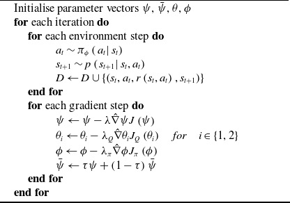
This paper develops a 3D dynamic environment for investigating real-time UAV obstacle avoidance, in which dynamic obstacles are modeled as spheres of varying radii moving along predefined trajectories at different velocities. To enhance motion realism, we implemented continuous UAV control through variable manoeuver commands, with the reinforcement learning framework generating continuous 3D velocity adjustments. Figure 1 illustrates the proposed model architecture.
The framework of the RL-based obstacle avoidance method.

The UAV navigation task requires reaching a randomly positioned target point
 $goal = [{x_g},{y_g},{z_g}]$
from a random start point
 $start = [{x_s},{y_s},{z_s}]$
near the environment boundary in 3D space, while avoiding collisions with dynamic obstacles and maintaining safe distance from boundaries. The UAV operates under partial observability, relying solely on limited detection sectors for environmental perception rather than complete obstacle position and velocity information. This observation scheme introduces perception uncertainty, leading researchers to model the DOA problem as a Partially Observable Markov Decision Process (POMDP). The POMDP framework formally describes the problem using the tuple
 $\left( {S,A,T,R,\Omega ,{\rm O}} \right)$
, where:
 $S = \left\{ {{s_1}, \cdots {s_n}} \right\}$
represents the state space,
 $A = \left\{ {{a_1}, \cdots {a_n}} \right\}$
denotes the action space, the state transition function
 $T\left( {s,a,s'} \right) = P\left( {s'|s,a} \right)$
specifies the probability of moving to state
 $s'$
when taking action
 $a$
in state
 $s$
.
 $R = r(s,a)$
indicates the reward function. The agent directly optimises policy
 ${\pi _\theta }\left( {a|s} \right)$
for obstacle avoidance decisions, with cumulative return is defined as
 \begin{align}J\left( \theta \right) = {{\mathbb E}_{\tau \sim {\pi _\theta }}}\left[ {\sum\limits_{t = 0}^\infty {{\gamma ^t}R\left( {{s_t},{a_t}} \right)} } \right]\end{align}
Under policy
 ${\pi _\theta }$
, the state-value function represents the expected cumulative discounted reward starting from state
 $s$
.
 \begin{align}{V^\pi }\left( s \right) = {{\mathbb E}_\pi }\left[ {J\left( \theta \right)|{s_t} = s} \right] = {{\mathbb E}_\pi }\left[ {\sum\limits_{t = 0}^\infty {{\gamma ^t}R\left( {{s_t},{a_t}} \right)|{s_t} = s} } \right]\end{align}
To evaluate the expected return when taking action
 $a$
in state
 $s$
, we define the action-value function
 ${Q^\pi }\left( {s,a} \right)$
as:
 \begin{align}{Q^\pi }\left( {s,a} \right) = {{\mathbb E}_\pi }\left[ {J\left( \theta \right)|{s_t} = s,{a_t} = a} \right] = {{\mathbb E}_\pi }\left[ {\sum\limits_{t = 0}^\infty {{\gamma ^t}R\left( {{s_t},{a_t}} \right)|{s_t} = s} ,{a_t} = a} \right]\end{align}
The optimal policy maximises the action-value function. For any state-action pair
 $\left( {s,a} \right)$
, we obtain
 ${\pi _\theta }$
by solving the Bellman Optimality Equation (BOE):
 \begin{align}{\pi ^*}\left( s \right) = \mathop {\arg \max }\limits_a {Q^\pi }\left( {s,a} \right),\forall s \in S,\forall a \in {\rm A} = \mathop {\arg \max }\limits_a {{\mathbb E}_\pi }\left[ {{r_t} + \gamma {Q^\pi }\left( {s',a'} \right)|{s_t} = s,{a_t} = a} \right]\end{align}
3.2 Motion model of UAV
Our research proposes a direct control method based on 3D-axis velocity to achieve continuous altitude and speed variations for UAVs in three-dimensional environments. Precise attitude control is enabled through dynamic adjustment of velocity components along three spatial axes. The UAV’s heading is automatically aligned with the resultant velocity vector to ensure motion continuity and flight stability.
To better simulate realistic tracking and avoidance manoeuvers, constraints were imposed on climbing, descending and turning operations. Based on UAV kinematic characteristics, a kinematic model incorporating dual constraints on both azimuth and climbing angles was developed, as shown in Fig. 2. Firstly, the UAV’s position at current time step is
 ${q_t} = ({x_t},{y_t},{z_t})$
, with its previous position is
 ${q_{before}} = ({x_{t - 1}},{y_{t - 1}},{z_{t - 1}})$
and the next position is
 ${q_{next}} = ({x_{t + 1}},{y_{t + 1}},{z_{t + 1}})$
. The azimuth angle
 $\phi $
calculated from the horizontal projection of position vectors, quantifies the heading change in horizontal plane, as shown in Equations (5) and (6).
 \begin{align}{\phi _0} = \arctan \left( {\frac{{\Delta {q_y}}}{{\Delta {q_x}}}} \right) = \arctan \left( {\frac{{{y_t} - {y_{t - 1}}}}{{{x_t} - {x_{t - 1}}}}} \right)\end{align}
 \begin{align}{\phi _1} = \arctan \left( {\frac{{\Delta {q_{next}}_y}}{{\Delta {q_{next}}_x}}} \right) = \arctan \left( {\frac{{{y_{t + 1}} - {y_t}}}{{{x_{t + 1}} - {x_t}}}} \right)\end{align}
UAV kinematic model.

Climbing angle characterises the movement trend of the UAV in the vertical direction, as shown in Equations (7) and (8).
 \begin{align}{\varphi _0} = \arctan \left( {\frac{{\Delta {q_{\rm{z}}}}}{{\Delta {q_{xy}}}}} \right) = \arctan \left( {\frac{{{z_t} - {z_{t - 1}}}}{{\sqrt {{{\left( {{x_t} - {x_{t - 1}}} \right)}^2} + {{\left( {{y_t} - {y_{t - 1}}} \right)}^2}} }}} \right)\end{align}
 \begin{align}{\varphi _1} = \arctan \left( {\frac{{\Delta {q_{next}}_{\rm{z}}}}{{\Delta {q_{next}}_{xy}}}} \right) = \arctan \left( {\frac{{{z_{t + 1}} - {z_t}}}{{\sqrt {{{\left( {{x_{t + 1}} - {x_t}} \right)}^2} + {{\left( {{y_{t + 1}} - {y_t}} \right)}^2}} }}} \right)\end{align}
The maximum azimuth angle
 $\Delta \phi $
limits abrupt heading changes within unit time. The adjusted yaw angle
 ${\phi _{res}}$
follows Equation (9).
 \begin{align}\left\{ \begin{array}{l}{\phi _{res}} = {\phi _1},\quad if\left| {{\phi _1} - {\phi _0}} \right| \le \Delta \phi \\[5pt]{\phi _{res}} = {\phi _0} + sign\left( {{\phi _1} - {\phi _0}} \right) * \Delta \phi ,\quad else\end{array} \right.\end{align}
The climbing angle constraints comprise rate constraints and physical limits. The rate constraint (Equation 10) maintains smooth vertical motion by restricting the climbing angle’s change rate. The physical constraint (Equation 11) enforces UAV performance limits through bounded climbing angle and diving angle.
 \begin{align}{\varphi _{res}} = \left\{ \begin{array}{l}{\varphi _1},\quad \left| {{\varphi _1} - {\varphi _0}} \right| \le \Delta \varphi \\[5pt]{\varphi _0} + sign\left( {{\varphi _1} - {\varphi _0}} \right) * \Delta \varphi ,\quad \left| {{\varphi _1} - {\varphi _0}} \right| \gt \Delta \varphi \end{array} \right.\end{align}
 \begin{align}{\varphi _{res}} = \max \left( {{\varphi _{\min }},\min \left( {{\varphi _{res}},{\varphi _{\max }}} \right)} \right)\end{align}
Where
 ${\varphi _{\max }}$
denotes the maximum climbing angle,
 ${\varphi _{\min }}$
represents the maximum diving angle.
3.3 Target tracking and dynamic obstacles avoidance model based On DRL
The UAV DOA problem is formulated as a Markov process, as illustrated in Fig 3. The environment is modeled in three-dimensional space and populated with multiple dynamic obstacles of different radii and motion patterns, providing diverse conditions for evaluating strategies. At each decision step, obstacle intrusions and target status are detected within the UAV’s sensor range, and the current state is updated accordingly. Conditioned on this observed state and constrained by UAV kinematics, the policy network trained with reinforcement learning selects avoidance actions in the form of incremental velocity adjustments. These actions continuously update the UAV trajectory in a stepwise manner, enabling the agent to react adaptively to dynamic obstacles until the mission is successfully accomplished at the target location.
Autonomous UAV obstacle avoidance model.

3.3.1 State space
The UAV obstacle avoidance task fundamentally involves searching for an optimal collision-free path. Our system processes three primary perception data types: the UAV internal state, intruding dynamic obstacle information and target-relative positioning. UAV internal state is characterised by triaxial velocity components
 $v = [{v_x},{v_y},{v_z}]$
, while its target-relative position is denoted by vector
 $\theta = {p_{goal}} - p$
. For three-dimensional environment perception, we propose a modular partial observation model [Reference Chen27] as shown in Fig. 4. The UAV observes a cylindrical region centred at its current position with detection radii
 ${R^D}$
and height
 $2{R^H}$
. When
 ${z_{obstacle}} - z \le {R^H}$
, the system registers obstacles occupying higher altitude layers
 ${k^u}$
, otherwise marked as
 ${k^l}$
. The detection zone is partitioned into n sectorial regions
 ${N_D}$
ordered relative to the UAV’s horizontal heading, yielding the obstacle observation matrix at timestep
 $t$
follows Equation (12).
 \begin{align}{o_t} = \left[ \begin{array}{l}o_t^{{k^u},1} \cdots o_t^{{k^u},{N_D}}\\[5pt]o_t^{{k^l},1} \cdots o_t^{{k^l},{N_D}}\end{array} \right]\end{align}
UAV obstacle detection model.

The intrusion distance is defined as the distance from the UAV to an obstacle’s surface. We calculate vertical
 $h$
and horizontal
 $d$
projections of through sine and cosine operations of their relative angles. The system registers an obstacle intrusion only when
 $h \le {R^H}\ \textrm{and}\ d \le {R^D}$
, enabling UAV perception. The classification of obstacles based on UAV detection states divides them into three categories. If an obstacle does not intrude, it is marked as undetected. When two obstacles appear in the same detection sector, the UAV only observes the one with the closest intrusion distance. Specifically, if an obstacle intrudes into two detection sectors, it is only counted in the sector containing its closest surface point.
3.3.2 Action space
To enable continuous variations in UAV altitude and speed within three-dimensional environments, this work directly controls the UAV’s 3D-axis velocity. The UAV’s heading always aligning with its velocity direction. The proposed DRL framework learns the 3D-axis velocity increments, which represent the action output
 $a = [\Delta {v_x},\Delta {v_y},\Delta {v_z}]$
at each timestep, allowing the UAV’s velocity and position updates to be expressed by Equation (13).
 \begin{align}\left\{ \begin{array}{l}v_x^{t + 1} = v_x^t + \Delta {v_x}\\[5pt]v_y^{t + 1} = v_y^t + \Delta {v_y}\\[5pt]v_z^{t + 1} = v_z^t + \Delta {v_z}\\[5pt]{x_{t + 1}} = {x_t} + v_x^{t + 1}\Delta t\\[5pt]{y_{t + 1}} = {y_t} + v_y^{t + 1}\Delta t\\[5pt]{z_{t + 1}} = {z_t} + v_z^{t + 1}\Delta t\end{array} \right.\end{align}
The variable
 $({x_t},{y_t},{z_t})$
represents the UAV’s position at timestep
 $t$
, while
 $\Delta t$
denotes the time interval between consecutive velocity control commands sent to the UAV, with a default value of 0.1 seconds. This short timestep interval enables continuous and smooth UAV control.
3.3.3 Reward
The reward value serves as the key mechanism for guiding UAV obstacle avoidance and target approach. We design a reward function to continuously incentivise UAV behaviour, consisting of four components: a sparse reward function, distance function, yaw function and speed function. The sparse reward function incorporates obstacle avoidance rewards, target rewards and boundary rewards as specified in Equation (14). During operation, the UAV receives penalties for colliding with obstacles or exiting the operational area. Additionally, the system imposes minor penalties when the UAV-obstacle distance falls below a buffer threshold to encourage timely evasion. When the UAV completes an action at each timestep, it obtains the full reward if reaching within the target threshold distance, thereby completing the episode. Otherwise, penalties are assessed based on the remaining distance to target when maximum episode steps are reached.
 \begin{align}{R_{sparse}} = {R_{avoid}} + {R_{goal}} + {R_{boundary}}\end{align}
 \begin{align}{R_{avoid}} = \left\{ \begin{array}{l}\frac{{\left\| {{P_{uav}} - {P_{obs}}} \right\|}}{{{r_{obs}}}} - {C_0},\quad 0 \le \left\| {{P_{uav}} - {P_{obs}}} \right\| \le {r_{obs}}\\[5pt]\frac{{\left\| {{P_{uav}} - {P_{obs}}} \right\|}}{{{r_{obs}} + {r_{buffer}}}} - {C_1},\quad {r_{obs}} \le \left\| {{P_{uav}} - {P_{obs}}} \right\| \le {r_{buffer}}\end{array} \right.\end{align}
 \begin{align}{R_{goal}} = \left\{ \begin{array}{l}C,{\rm{ 0}} \le \left\| {{P_{goal}} - {P_{uav}}} \right\| \le threshold\\[5pt]\max \left(c, - \frac{{\left\| {{P_{goal}} - {P_{uav}}} \right\|}}{{{d_{boundary}}}}\right),\quad else\end{array} \right.\end{align}
While sparse rewards prove insufficient for effective UAV mission completion, we augment the reward system with dense rewards comprising distance and yaw functions. These functions operate at every timestep to progressively guide the UAV toward the target point, as specified in Equations (17) and (18). The distance function combines two key components: it simultaneously encourages target approach while maintaining altitude constraints. Specifically, the UAV receives incentives for reducing target distance at each step, but is penalised for exceeding permissible altitude boundaries.
 \begin{align}{R_d} = \left(1 - \frac{{\left\| {P_{goal}^{} - P_{uav}^{t + 1}} \right\|}}{{\left\| {P_{goal}^{} - P_{uav}^t} \right\|}}\right) + \lambda \left\| {z_{goal}^t - z_{uav}^t} \right\|\end{align}
 \begin{align}{R_{{\rm{yaw}}}} = \lambda \cdot \frac{{\left| \phi \right|}}{\pi }\end{align}
The speed function constrains the UAV’s velocity within performance limits, imposing penalties when the resultant speed exceeds the maximum threshold as specified in Equation (19).
 \begin{align}{R_{speed}} = \lambda \cdot \frac{{v - {v_{\max }}}}{{{v_{\max }}}}\end{align}
Integrating all aforementioned reward components yields the complete reward function shown in Equation (20).
 \begin{align}R = {R_{sparse}} + {R_d} + {R_{{\rm{yaw}}}} + {R_{speed}}\end{align}
3.4 Soft Actor-Critic
This study employs the Soft Actor–Critic (SAC) algorithm, which integrates the Actor–Critic framework with policy gradient methods. In the conventional Actor–Critic architecture, the actor network generates candidate actions according to the current policy, while the critic network evaluates these actions by estimating their expected return through a value function. SAC extends this architecture by introducing the maximum entropy reinforcement learning framework, where the optimisation objective consists not only of the cumulative return but also an additional entropy term, thereby explicitly encouraging stochasticity in action selection. By balancing reward maximisation with entropy maximisation, SAC facilitates more effective exploration, prevents premature convergence to suboptimal deterministic solutions and enhances robustness in highly dynamic or uncertain environments. Information entropy, which serves as a measure of uncertainty in action selection, is formally defined in Equation (21).
 \begin{align}{\rm H}\left( x \right) = {{\mathbb E}_{x \sim P}}\left( { - \log P\left( x \right)} \right)\end{align}
The entropy-maximised policy objective becomes Equation (22), where
 ${\rho _\pi }$
represents the state-action pair distribution encountered by the agent under policy
 $\pi $
. The temperature coefficient serves as a hyperparameter that regulates the emphasis on entropy maximisation
 \begin{align}{\pi ^*} = \mathop {\mathop {\arg \max }\limits_\pi } \,\mathbb{E}_{\left( {s_t},{a_t} \right) \sim {\rho _\pi }} \left[ {\sum\limits_t {r\left( {{s_t},{a_t}} \right) + \alpha {\rm H}\left( {\pi \left( {\left. \cdot \right|{s_t}} \right)} \right)} } \right]\end{align}
Traditional reinforcement learning aims to maximise the expected cumulative reward as shown in Equation (1). In contrast, SAC introduces an entropy term that incorporates a policy randomness weight into the reward function, as specified in Equation (23).
 \begin{align}J\left( \theta \right) = {{\mathbb E}_{\tau \sim {\pi _\theta }}}\left[ {\sum\limits_{t = 0}^\infty {{\gamma ^t}R\left( {{s_t},{a_t}} \right) + \alpha H\left( {\pi \left( {\left. \cdot \right|{s_t}} \right)} \right)} } \right]\end{align}
 $H\left( {\pi \left( {\left. \cdot \right|{s_t}} \right)} \right)$
quantifies the randomness level of policy
 $\pi $
in state
 $s$
.
The pseudocode of the SAC algorithm 1 is presented above.
Soft Actor-Critic

4.0 Results and Discussion
4.1 Training scenarios
This study establishes a three-dimensional simulation environment of
 $400\,\textrm{m} \times 400\,\textrm{m} \times 100\,\textrm{m}$
on the Python platform. The scene contains four spherical dynamic obstacles with a radius of 15 m. The centres of these obstacles vary with time, creating a continuously evolving collision risk during flight. At the beginning of each episode, obstacles are randomly placed in the workspace and assigned random motion phases. The UAV is initialised near the boundary and directed toward a target located on the boundary. An episode is counted as successful when the UAV reaches a 10 m neighbourhood of the target. To span diverse motion patterns, obstacle trajectories are drawn from parametric families, including circular and elliptical orbits at constant altitude or with vertical oscillation, as well as reversible piecewise periodic paths. These motions are deterministic functions of time and initial phase. Equation (24) specifies the trajectory of an obstacle executing circular motion at constant altitude.
 \begin{align}c(t) = {c_0} + [R\cos (\omega t + \varphi ),R\sin (\omega t + \varphi ),h]\end{align}
Here,
 $\omega $
denotes the angular rate,
 $h$
denotes the constant altitude,
 $t$
is the simulation time, and
 $R$
is the orbit radius. The instantaneous velocity is the time derivative
 $c(t)'$
. In this study, we design eight types of obstacle motion trajectories; at each initialisation, four moving obstacles are randomly sampled to construct the training scenario. The UAV receives only instantaneous observations within a bounded sensing range, such as the current position and bearing of visible obstacles, and no information about their future trajectories.
4.2 Parameter setting
4.2.1 Experiments setup
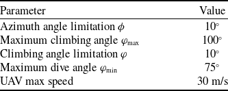
In this experiment, the UAV operates with a 20-m detection radii and height, divided into eight detection sectors. The timestep is set to 0.1 s, with kinematic constraints detailed in Table 1.
Kinematic constraint parameters

4.2.2 Performance index
To evaluate model performance, five metrics are adopted: extra flight distance, threat index (TI), path tortuosity, average steps (AS), success rate and average reward. The success rate and reward value directly quantify the algorithm’s performance. A successful trial requires the UAV to reach the target collision-free within the maximum step limit. Superior models achieve the highest success rates, demonstrating unequivocal performance advantages. The average reward comprehensively evaluates navigation accuracy, obstacle avoidance safety, and motion efficiency, with higher values indicating superior overall performance. The AS measures algorithmic efficiency, where lower values correspond to faster mission completion. Extra flight distance is defined as the difference between the UAV’s actual path length in each episode and the Euclidean distance between its start and end points. Path length calculation follows Equation (25), where n represents the total number of waypoints and
 ${q_i} = \left( {{x_i},{y_i},{z_i}} \right)$
denotes the UAV position at timestep t. The extra flight distance is computed as specified in Equation (26). This metric evaluates trajectory economy, with shorter paths corresponding to lower energy consumption. The TI assesses collision risks during navigation, while path tortuosity measures trajectory smoothness through angular deviation analysis.
 \begin{align}L = \sum\limits_{i = 0}^{n - 2} {\sqrt {{{\left( {{x_{i + 1}} - {x_i}} \right)}^2} + {{\left( {{y_{i + 1}} - {y_i}} \right)}^2} + {{\left( {{z_{i + 1}} - {z_i}} \right)}^2}} } \end{align}
 \begin{align}{L_{extra}} = L - \sqrt {{{\left( {{x_{n - 1}} - {x_0}} \right)}^2} + {{\left( {{y_{n - 1}} - {y_0}} \right)}^2} + {{\left( {{z_{n - 1}} - {z_0}} \right)}^2}} \end{align}
The TI, as defined in Equation (27), quantifies the UAV’s obstacle avoidance performance, where
 ${d_i}$
represents the real-time distance between the UAV and the i-th obstacle, and N denotes the total number of obstacles (set as N = 4 during training). Lower TI values indicate reduced collision risk between the UAV and obstacles.
 \begin{align}TI = \sum\limits_{i = 1}^N {\left\{ \begin{array}{l}100\quad if\quad {d_i} \le 0\\[5pt]\frac{{10}}{{{d_i}}}\quad if\quad {\rm{ 0}} \lt {d_i} \le 10\\[5pt]0\quad if\quad {d_i} \gt 10\end{array} \right.} \end{align}
The path tortuosity metric comprises two components: global tortuosity (GS) and local maximum tortuosity (LS), as defined in Equations (28) and (29), respectively.
 \begin{align}GS = \frac{1}{n}\sum\limits_{i = 1}^n {\left( {{\mu _1} \cdot \Delta {\phi _i} + {\mu _2} \cdot \Delta {\varphi _i}} \right)} \end{align}
 \begin{align}LS = \mathop {\max }\limits_i \left( {{\mu _1} \cdot \Delta {\phi _i} + {\mu _2} \cdot \Delta {\varphi _i}} \right)\end{align}
The variables
 $\Delta {\phi _i}$
and
 $\Delta {\varphi _i}$
represent the yaw angle change and climb angle change, respectively. GS measures the overall path smoothness, where smaller values indicate gradual UAV turns and larger values suggest frequent aggressive manoeuvers with unstable control. LS quantifies the severity of local turns, with lower values demonstrating absence of sharp turns or sudden pitch variations.
Comparison of obstacle avoidance trajectory.

4.3 Experimental results
To demonstrate the effectiveness of the proposed method in dynamic multi-obstacle avoidance scenarios, this paper presents UAV flight trajectories across six distinct obstacle configurations, as illustrated in Fig. 5. Each scenario contains four obstacles with different motion patterns, while maintaining fixed start and target positions for the UAV. The baseline trajectory shows the UAV moving toward the target at constant speed, consistently exhibiting collision points. Under identical environmental conditions, tests conducted with the trained avoidance model successfully eliminate all collision points in the avoidance trajectories, confirming the model’s effectiveness. Experimental results reveal noticeable differences between obstacle trajectories before and after avoidance, attributable to the UAV’s dual strategy of both path deviation and proactive speed adjustment to maintain safe distances before potential collisions, thereby achieving earlier target arrival.
4.4 Comparison experiment
4.4.1 Training curve
This study presents a comparative performance analysis of the proposed UAV autonomous obstacle avoidance method against four baseline algorithms: SAC, Twin Delayed Deep Deterministic Policy Gradient (TD3), Squashed Twin Delayed Deep Deterministic Policy Gradient (SD3) and Deep Deterministic Policy Gradient (DDPG). Figure 6 illustrates the reward function training curves, revealing the performance evolution of each algorithm during training. All experiments were conducted over 20k training episodes, with systematic reward evaluation performed after each episode. The results indicate that all four algorithms converge within the 20k episode training period, confirming their operational effectiveness.
Training curves of different obstacle avoidance algorithms.

Figure 7 displays the convergence characteristics of extra flight distance across all four algorithms during training. This metric serves as a critical performance indicator for UAV obstacle avoidance systems, providing quantitative assessment of trajectory efficiency during avoidance manoeuvers.
4.4.2 Performance comparison
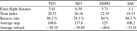
The trained model was evaluated through 1000 simulation trials with randomised start-target configurations in the training environment. Table 2 presents the averaged evaluation metrics from these tests. Performance evaluation based on average reward values demonstrates the SAC algorithm’s superiority over baseline methods. Furthermore, the SAC model achieves shorter extra flight distances and fewer average steps than competing algorithms, confirming its enhanced economic efficiency.
The algorithm’s adaptability to transferred environments is evaluated through the following validation tests. Differentiated test scenarios are constructed by varying the number of obstacles and their radii, enabling comparison of the algorithm’s comprehensive performance when facing obstacles of different scales. Figure 8 shows the evaluation results using success rate and average reward values. In scenarios with large obstacles, the SAC algorithm maintains higher success rates than comparative algorithms. Its average reward values consistently outperform benchmarks, demonstrating the model’s ability to ensure both safety and economic efficiency simultaneously. Notably, the algorithm’s overall performance remains stable without abrupt degradation when encountering large obstacles.
Comparative results of evaluation metrics

Training extra flight distances of different obstacle avoidance algorithms.

Comprehensive performance evaluation of models.

The trained algorithms’ performance is analysed from two perspectives: safety and efficiency. Efficiency is measured by both the average steps required for mission completion and extra flight distance, while safety is assessed through TI evaluation. This framework allows direct comparison of different algorithms’ overall performance characteristics. As shown in Fig. 9, the TI varies under environment transfer conditions. Increasing either obstacle quantity or size raises environmental complexity, leading to higher threat indices. The proposed method maintains consistently lower TI values without dangerous abrupt surges, demonstrating robust safety performance across all scenarios.
Safety performance assessment results.

Figure10 shows the distribution of additional flight distances in transferred scenarios. The results indicate a progressive increase in additional flight distance corresponding to both obstacle quantity and radii. Notably, the SAC algorithm maintains significantly lower maximum additional distances and tighter distribution ranges compared to baseline methods. This advantage becomes particularly evident in complex environments, where SAC exhibits slower growth rates in additional flight distance, demonstrating superior stability.
Extra flight distance distribution in a migration environment.

The average step count serves as a direct measure of UAV travel efficiency between origin and destination. When operating in environments containing numerous or large obstacles, additional navigation steps are required to ensure safe obstruction avoidance. Figure 11 demonstrates that the proposed method maintains controlled step count growth while preserving safety, achieving an optimal balance between operational economy and security needs. Comparative results show that although SD3 and DDPG algorithms produce shorter average paths, they are accompanied by TI fluctuations. Path folding analysis (GS and LS) confirms that these algorithms compromise obstacle avoidance capability through excessive path smoothing, leading to safety degradation during large obstacle encounters.
4.5 Sensitivity analysis
The quantity of detection sectors in the proposed observation matrix constitutes a crucial parameter for this model. The modular observation matrix improves UAV perception of obstacle, while excessive sector partitioning elevates the computational for data processing. Figure 12 displays the training results for various detection sector configurations, illustrating the trade-off between environmental perception and processing efficiency.
Economic performance assessment results.

Training curves for different detection number models.

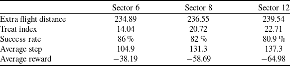
The experimental results clearly demonstrate the unsuccessful training of models without modular observation matrices. As the number of detection sectors increases, the model begins to achieve convergence. However, excessive sector partitioning introduces substantial redundant information, leading to learning instability and noticeable fluctuations in training curves. Table 3 presents the performance evaluation results for models with different numbers of detection sectors, quantitatively illustrating this optimisation trade-off.
The results indicate optimal model performance occurs with six detection sectors. This phenomenon likely stems from the non-negligible physical dimensions of obstacles, which cannot be simplified as point masses. Excessive detection modules may cause obstacles to occupy multiple adjacent sectors, ultimately impairing the UAV’s ability to accurately determine their precise position. Furthermore, increasing the observation space dimensionality not only introduces redundant information but also elevates model complexity, creating additional learning challenges.
5.0 Conclusion
This study proposes a dynamic obstacle avoidance method for low-altitude UAVs that combines SAC reinforcement learning with kinematic performance constraints. The proposed modular observation space significantly improves UAV obstacle perception in highly dynamic environments, while simultaneously enhancing data efficiency and accelerating model convergence. This solution effectively addresses critical safety challenges posed by large-scale, highly dynamic obstacles in real-world operations.
Extensive simulations demonstrate the trained SAC model’s superior performance in extra flight distance, convergence efficiency, average steps, TI and comprehensive evaluation metrics. The experiments also validate the effectiveness of the designed state space and action space configurations.
Sensitivity analysis for detection number

While acknowledging that real-world conditions exceed experimental complexity, this research will extend the simulation environment by integrating visual and distance sensors to better approximate actual operational conditions. Future investigations will focus on reducing this reality gap while preserving the method’s computational efficiency and safety guarantees.
Acknowledgments
The work described in this article was supported by Aeronautical Science Foundation of China (grant 20240055052003) and Shenzhen Longhua Science and Technology Innovation Special Funding Project (Industrial Sci-Tech Innovation Center of Low-Altitude Intelligent Networking) (grant SZRI-2025-02).