

Adolescence is a developmental period characterized by increases in risk behaviors, mood fluctuations, and conflict with parents (Arnett, Reference Arnett1992, Reference Arnett1999), as well as when significant brain development occurs in the frontal lobes, influencing the development of better reasoning and decision-making capabilities (Dahl, Reference Dahl2004; Reyna & Farley, Reference Reyna and Farley2006). Recent national data from the 2005 Youth Risk Behavior Survey (Eaton et al., Reference Eaton, Kann, Kinchen, Ross, Hawkins and Harris2006) highlight that a substantial percentage of adolescents in 9th through 12th grades in the United States are involved in a number of risk behaviors, including current cigarette smoking (23.0%), alcohol use (43.3%), heavy drinking (25.5%), marijuana use (20.2%), aggression and violence (e.g., physical fighting; 35.9%), and extreme feelings of sadness (28.5%) and suicidal ideas (16.9%). The alarmingly high rates of substance use among adolescents and college students are echoed in the most recent report from the Monitoring the Future National Survey (Johnston, O'Malley, Bachman, & Schulenberg, Reference Johnston, O'Malley and Bachman2006). For most adolescents, engagement in some level of risk behavior is part of a statistically normative process that is intertwined with age-appropriate developmental tasks associated with increases in autonomy and self-regulation.
However, researchers agree that there exist subsets of adolescents at elevated risk whose adolescent-typical behaviors may represent atypical developmental processes, and it remains a critical task to detect atypical symptomatic processes from the normative pathway in the field of developmental psychopathology (Cicchetti & Rogosch, Reference Cicchetti and Rogosch2002). Evidence of heterogeneity in developmental pathways consisting of normative as well as atypical processes can be found in depressive disorders and symptoms (Cicchetti & Toth, Reference Cicchetti and Toth1998; Kim, Capaldi, & Stoolmiller, Reference Kim, Capaldi and Stoolmiller2003; Stoolmiller, Kim, & Capaldi, Reference Stoolmiller, Kim and Capaldi2005), heavy drinking (Schulenberg, O'Malley, Bachman, Wadsworth, & Johnston, Reference Schulenberg, O'Malley, Bachman, Wadsworth and Johnston1996; Windle, Mun, & Windle, Reference Windle, Mun and Windle2005), smoking (Chassin, Presson, Pitt, & Sherman, Reference Chassin, Presson, Pitt and Sherman2000; Chassin, Presson, Sherman, & Edwards, Reference Chassin, Presson, Sherman and Edwards1991; Shiffman, Kassel, Paty, Gnys, & Zettler-Segal, Reference Shiffman, Kassel, Paty, Gnys and Zettler-Segal1994), alcohol and drug use (Chassin, Flora, & King, Reference Chassin, Flora and King2004), antisocial behavior (Moffitt, Reference Moffitt1993; Nagin, Farrington, & Moffitt, Reference Nagin, Farrington and Moffitt1995), and aggression (Bongers, Koot, van der Ende, & Verhulst, Reference Bongers, Koot, van der Ende and Verhulst2004; Brame, Nagin, & Tremblay, Reference Brame, Nagin and Tremblay2001; Loeber & Stouthamer-Loeber, Reference Gorman-Smith, Tolan, Loeber and Henry1998). From this corpus of research, variations in onset and desistance, as well as overall levels of the behaviors, have been identified as critical factors for identifying individuals at risk. In these studies, researchers found that the adolescents who are flagged for early onset tend to also show other elevated behavior problems and concurrent clinical symptoms. Thus, it is critical to identify adolescents who are at increased risk for developmental pathways marked by a prolonged period of multiple dysfunctions from other less risky or singular-problem pathways, and to understand how vulnerability develops and is expressed across time.
Cluster Analysis for Identifying Adolescents at Risk
A number of other studies have identified clusters of adolescents who can be distinguished from others based on behavioral domains and/or substance use (Crockett, Moilanen, Raffaelli, & Randall, Reference Crockett, Moilanen, Raffaelli and Randall2006; Gorman-Smith, Tolan, Loeber, & Henry, Reference Gorman-Smith, Tolan, Loeber and Henry1998; Haselager, Cillessen, Van Lieshout, Riksen-Walraven, & Hartup, Reference Haselager, Cillessen, Van Lieshout, Riksen-Walraven and Hartup2002; Miller & Plant, Reference Miller and Plant2002; Potter & Jenson, Reference Potter and Jenson2003; Tubman, Vicary, von Eye, & Lerner, Reference Tubman, Vicary, von Eye and Lerner1990). Although these studies have provided valuable insight into heterogeneous clusters of adolescents who vary on problem behaviors, major methodological limitations are twofold. First, the cluster analyses conducted in these studies used either a limited number of problem behaviors (Miller & Plant, Reference Miller and Plant2002), a small sample size (Tubman et al., Reference Tubman, Vicary, von Eye and Lerner1990), and/or consisted of a highly selective sample such as juvenile offenders (Potter & Jenson, Reference Potter and Jenson2003). Second, and more critically, the cluster analytic techniques used in these studies are considered to have substantial weaknesses. In particular, these clustering algorithms' lack of a statistical fit measure to determine the adequacy of the number of clusters, yields indeterminacy of a cluster solution (Dumenci & Windle, Reference Dumenci and Windle2001; Tonidandel & Overall, Reference Tonidandel and Overall2004), and the clustering solution may be influenced by the order of data input (van der Kloot, Spaans, & Heiser, Reference van der Kloot, Spaans and Heiser2005). These issues are compounded, given that each clustering method has unique tendency to favor a certain solution. For instance, Ward's method, one of the most commonly used clustering methods, tends to result in spherical clusters of the same size (for more detail, see Everitt, Landau, & Leese, Reference Everitt, Landau and Leese2001; von Eye, Mun, & Indurkhya, Reference von Eye, Mun and Indurkhya2004). Furthermore, spurious clusters can be artificially created by a clustering method that imposes a structure on the data even when there are no true clusters (Everitt et al., Reference Everitt, Landau and Leese2001; von Eye & Bergman, Reference von Eye and Bergman2003; von Eye et al., Reference von Eye, Mun and Indurkhya2004). Although a series of careful decisions (e.g., hierarchical vs. nonhierarchical clustering procedures, deterministic vs. stochastic clustering, choosing a linkage method, and deciding on including or excluding outliers) can limit the arbitrariness involved in heuristic clustering procedures (see von Eye et al., Reference von Eye, Mun and Indurkhya2004), findings based on subjective classification rules and means in finding cluster patterns should be viewed cautiously (Hand & Bolton, Reference Hand and Bolton2004; Nagin, Reference Nagin2005).
Mixture Model-Based Cluster Analysis Using Finite Mixture Distributions
Newly emerging model-based cluster analysisFootnote 1 utilizes finite mixture densities (Everitt, Reference Everitt, Everitt and Howell2005; Everitt & Hand, Reference Everitt and Hand1981; McLachlan & Peel, Reference McLachlan and Peel2000). The foci of clustering become that of estimating (a) the parameters of the assumed mixture (e.g., multivariate normal, multivariate t, multivariate multinomial, etc.) and (b) the posterior probabilities of cluster membership (Banfield & Raftery, Reference Banfield and Raftery1993; Everitt et al., Reference Everitt, Landau and Leese2001). This analytic approach targets the identification of unobserved heterogeneity in a population based on the observed data. Model-based cluster analysis assumes that the distribution is made up of a number of multivariate component distributions (typically normal densities), and it utilizes the expectation–maximization (EM) algorithm for maximum likelihood (ML) estimation. The ultimate goal of model-based cluster analysis is similar to any of the heuristic clustering algorithms such as hierarchical agglomerative or the k-means clustering method. It aims to find a number of salient groups of objects (e.g., individuals, genes, etc.) that are similar to one another within a group but sufficiently different from members of other groups. However, mixture model-based cluster analysis is different from the existing heuristic clustering procedures in that it employs the explicit assumption that a population can be approximated as a weighted sum of component distributions a priori unknown and unobserved, which can be interpreted as evidence of distinctive subgroups or heterogeneity in a population. In addition, the cluster membership of an individual is expressed as a probability (range = 0–1), as opposed to hard, deterministic classification that typically assumes that cluster membership of an individual equals 1.
This emerging approach to cluster analysis via a finite mixture model has been better known and utilized in the field of gene expression data (McLachlan, Do, & Ambroise, Reference McLachlan, Do and Ambroise2004). To our knowledge, however, this model-based cluster analysis approach has not been introduced in the field of developmental psychopathology. Latent class analysis, latent class growth curve analysis, and latent class regression using the Mplus program (Muthén & Muthén, Reference Muthén and Muthén1998–2006) can be considered as types of model-based cluster analysis as well (Everitt et al., Reference Everitt, Landau and Leese2001). From a different angle, mixture model-based cluster analysis can be viewed as a type of hybrid latent variable analysis with no measurement invariance and nonparametric factor distribution (i.e., nonparametric factor mixture analysis; Muthén, Reference Muthén2006). If a component in finite mixture densities is considered as a latent class (e.g., Dolan, Schmittmann, Lubke, & Neale, Reference Dolan, Schmittmann, Lubke and Neale2005; see Bollen, Reference Bollen2002, for in-depth discussion on various definitions of latent variables), the mixture model-based cluster analysis may also be understood as latent cluster analysis.
As expected, a mixture model-based cluster analysis has commonalities with recent methodological advances that utilize finite mixture distributions applied to structural equation models (Arminger & Stein, Reference Arminger and Stein1997; Arminger, Stein, & Wittenberg, Reference Arminger, Stein and Wittenberg1999; Dolan & van der Maas, Reference Dolan and van der Mass1998; Jedidi, Jagpal, & DeSarbo, Reference Jedidi, Jagpal and DeSarbo1997; Lubke & Muthén, Reference Lubke and Muthén2005) and longitudinal models (Muthén & Shedden, Reference Muthén and Shedden1999; Nagin, Reference Nagin1999, Reference Nagin2005). Especially the growth mixture modeling and latent class growth curve analysis techniques have sparked an avalanche of empirical studies that have identified and compared groups of individuals who follow particular developmental courses and compared them with other patterns of change groups in terms of the antecedents, correlates, and consequences of their developmental trajectories. These studies have shown evidence of heterogeneous developmental trajectories for smoking behavior (Chassin et al., Reference Chassin, Presson, Pitt and Sherman2000; Colder, Mehta, et al., Reference Colder, Mehta, Balanda, Campbell, Mayhew and Stanton2001; Orlando, Tucker, Ellickson, & Klein, Reference Orlando, Tucker, Ellickson and Klein2004; Tucker, Ellickson, & Klein, 2002; White, Pandina, & Chen, Reference White, Pandina and Chen2002), alcohol use (Chassin, Pitts, & Prost, Reference Chassin, Pitts and Prost2002; Colder, Campbell, Ruel, Richardson, & Flay, Reference Colder, Campbell, Ruel, Richardson and Flay2002; Hill, White, Chung, Hawkins, & Catalano, Reference Hill, White, Chung, Hawkins and Catalano2000; Tucker, Orlando, & Ellickson, Reference Tucker, Orlando and Ellickson2003; Windle et al., Reference Windle, Mun and Windle2005), marijuana use (Flory, Lynam, Milich, Leukefeld, & Clayton, Reference Flory, Lynam, Milich, Leukefeld and Clayton2004; Guo et al., Reference Guo, Chung, Hill, Hawkins, Catalano and Abbott2002; Windle & Wiesner, Reference Windle and Wiesner2004), depressive symptoms (Stoolmiller et al., Reference Stoolmiller, Kim and Capaldi2005; Windle & Mun, Reference Windle and Mun2006), and delinquent behavior (Nagin & Tremblay, Reference Nagin and Tremblay1999; Wiesner & Capaldi, Reference Wiesner and Capaldi2003; Wiesner, Kim, & Capaldi, Reference Wiesner, Kim and Capaldi2005).
Although these studies support heterogeneous subgroups in each of the problem behaviors previously mentioned, the rapidly growing literature has become difficult to synthesize because of its wide variation in measures (e.g., frequency versus quantity of substance use), sample characteristics (e.g., community-based normative samples versus high-risk samples), and analytic models (e.g., conditional vs. unconditional models). Moreover, past studies utilizing latent growth mixture analysis have typically considered a single problem behavior (e.g., delinquency) per study when deriving groups, thereby overlooking the co-occurrence of multiple problem behaviors that is common in adolescence, and consequently limiting the understanding of general and specific causal mechanisms responsible for heterogeneity of pathways and comorbidity. Although a few recent studies have derived groups based on joint or parallel trajectory models (Chassin et al., Reference Chassin, Flora and King2004; Jester et al., Reference Jester, Nigg, Adams, Fitzgerald, Puttler and Wong2005; Nagin & Tremblay, Reference Nagin and Tremblay1999), the scope of adolescent problem behaviors under investigation has been very limited in both number and kind. Furthermore, few existing studies of joint trajectories have investigated two closely related behaviors (Hix-Small, Duncan, Duncan, & Okut, Reference Hix-Small, Duncan, Duncan and Okut2004; Jester et al., Reference Jester, Nigg, Adams, Fitzgerald, Puttler and Wong2005).
The current study intends to fulfill two inseparable goals. We aim to introduce a mixture model-based cluster analysis approach and to derive meaningful clusters of adolescents with different risk profiles from the person-oriented and pattern-oriented approaches (Bergman & Magnusson, Reference Bergman and Magnusson1997; Magnusson, Reference Magnusson, Bergman, Cairns, Nilsson and Nystedt2000; von Eye & Bergman, Reference von Eye and Bergman2003). One typical assumption involved in the variable-oriented research is that all relevant contributing factors to an outcome be included so that each causal factor's contribution can be understood when effects of all other variables are controlled (i.e., at their means). However, an average score is often atypical and uninformative for research on developmental psychopathology, and can be misleading in some situations (von Eye & Bergman, Reference von Eye and Bergman2003). Furthermore, the entire model can be misleading if an important variable is excluded because the exclusion can potentially modify the entire network of relationships among variables. Another related assumption is that variable-oriented research attempts to identify common (“main effect”) causal relations that apply to all individuals (unless an a priori model is hypothesized to account for the specificity of targeted relations for different groups of individuals, i.e., interaction terms). Thus, our understanding of individual vulnerability and resilience with regard to adolescent problem behaviors and their consequences will benefit from the person-oriented research with a within-individual, person-oriented focus, especially because adolescent problem behaviors are well known to co-occur with high frequency and with a higher frequency among some adolescents relative to others. In the present study, we sought to empirically identify clusters of adolescents who differ in their profiles of multiple problem behaviors using a new nonparametric method called model-based cluster analysis and to understand precursors and correlates from middle adolescence to young adulthood.
The Current Study
We focused on identifying distinctive groups of adolescents with different kinds and/or levels of risk, and comparing the empirically derived cluster groups on adolescent temperamental and academic risk factors and young adult outcomes. Adolescent temperamental characteristics (e.g., Chassin et al., Reference Chassin, Flora and King2004; Tubman & Windle, Reference Tubman and Windle1995; Windle, Reference Windle1989, Reference Windle1991) and academic functioning (e.g., Jessor, van den Bos, Vanderryn, Costa, & Turbin, Reference Jessor, van den Bos, Vanderryn, Costa and Turbin1995) have been extensively studied as correlates of adolescent problem behaviors. Furthermore, temperamental deviations, in particular, have been strongly suggested (Moffitt, Reference Moffitt1993; Tarter & Vanyukov, Reference Tarter and Vanyukov1994; Zucker, Ellis, Bingham, & Fitzgerald, Reference Zucker, Ellis, Bingham and Fitzgerald1996; Zucker, Fitzgerald, & Moses, Reference Zucker, Fitzgerald, Moses, Cicchetti and Cohen1995) as an early indicator of neuropsychological risk that may be manifested as deficits in behavioral and emotional regulation and academic difficulties. More broadly, individual differences in temperament may signal different levels of behavioral and emotional self-regulation and reactivity in expressing one's self in socially acceptable ways (Posner & Rothbart, Reference Posner and Rothbart2000). A good number of publications have extended our understanding of early temperament in association with adult functioning and psychopathology (e.g., the Dunedin Multidisciplinary Health and Development Study), but relatively little attention has been given to more temporally proximal associations between adolescent measures and young adult functioning and psychopathology (Cicchetti & Rogosch, Reference Cicchetti and Rogosch2002; Schulenberg, Sameroff, & Cicchetti, Reference Schulenberg, Sameroff and Cicchetti2004). Finally, we examined whether derived clusters of adolescents were linked to young adult outcomes such as young adult substance use and abuse, depressive symptoms, overall perceived health, and education completed. High-risk groups of adolescents were hypothesized to have higher risk young adult profiles for the outcome measures in this study.
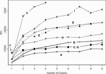
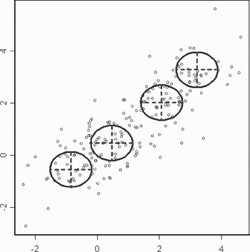
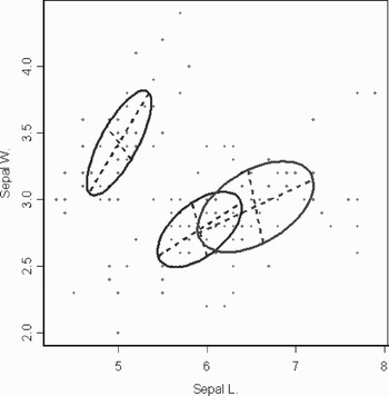
To cluster adolescents, we used the MCLUST program developed by Fraley and Raftery (Reference Fraley and Raftery1998, Reference Fraley and Raftery1999, Reference Fraley and Raftery2002a, Reference Fraley and Raftery2002b, Reference Fraley and Raftery2003) and designed for S-PLUS software program (version 6 or higher; Insightful Corporation, 1988–2006) and R language (available gratis at http://www.r-project.org/). This model-based clustering approach unambiguously postulates that a population consists of heterogeneous subpopulations that can differ in multidimensional data space calibrated in terms of volume (size of a cluster), orientation (an ellipsoid's orientation angles), and shape (a sphere or an ellipsoid). Appendix A provides graphic illustrations of volume, shape, and orientation in two-dimensional space. These geometric properties—volume, shape, and orientation—of a covariance matrix among observed variables are parameterized (see Appendix B for more information). A total of 10 possible models can be simultaneously compared using the Bayesian information criterion (BIC) as a statistical fit measure for the same number of extracted subcomponents (e.g., see Figure 1). The simplest model (Model A = same volume and shape, spherical clusters) has been shown to be very closely related to the k-means clustering algorithm (Celeux & Govaert, Reference Celeux and Govaert1992; Everitt et al., Reference Everitt, Landau and Leese2001; Yeung, Fraley, Murua, Raftery, & Ruzzo, Reference Yeung, Fraley, Murua, Raftery and Ruzzo2001). Because all models are compared at the same time using the BIC, a straightforward, statistical measure is available to draw a conclusion about the optimal number of clusters (e.g., component distributions) and the best clustering procedure reflected by the spatial characteristics of data. This is an important advantage of the MCLUST program because there generally exists a trade-off between the number of clusters and the number of estimated parameters. The more simplistic models may require a larger number of clusters to adequately fit the data, whereas a small number of clusters may be sufficient with increasingly more complex models to provide adequate fit to the data (Yeung et al., Reference Yeung, Fraley, Murua, Raftery and Ruzzo2001; for an empirical demonstration applied to, for instance, latent class growth trajectory analysis, see Bauer & Curran, Reference Bauer and Curran2003, Reference Bauer and Curran2004). After identifying cluster groups, we analyzed adolescent temperamental and academic profiles by cluster groups, and young adult function profiles by cluster groups.
Bayesian information criteria (BIC) of different cluster solutions. A, spherical, equal volume, equal shape; B, spherical, unequal volume, equal shape; C, diagonal, equal volume, equal shape; D, diagonal, unequal volume, equal shape; E, diagonal, equal volume, varying shape; F, diagonal, unequal volume, varying shape; G, ellipsoidal, equal volume, equal shape, equal orientation; H, ellipsoidal, equal volume, equal shape, varying orientation; I, ellipsoidal, unequal volume, equal shape, varying orientation; J, ellipsoidal, unequal volume, varying shape, varying orientation. The BIC for the J model was −16,056.65, the same BIC value as the Model I one cluster solution, and it stopped converging beginning at two clusters. [A color version of this figure can be viewed online at www.journals.cambridge.org]

Methods
Participants
The data used in this study were collected as part of a larger, multiwave panel design focused on vulnerability factors and adolescent and adult substance use (Lives across Time; Windle & Wiesner, Reference Windle and Wiesner2004). Of the maximum original sample of 1,205 adolescent participants (591 males, 614 females) who completed at least one of a maximum of four waves of adolescent assessment, we analyzed 1,126 participants (546 males, 580 females) who provided any information on the seven problem behaviors measured at Wave 2. The Wave 1 data collection during adolescence occurred during the fall semester of the teens' 10th- and 11th-grade years. Waves 2–4 data collection occurred every 6 months thereafter, with Wave 2 data being collected in the spring semester of Year 1, and Waves 3 and 4 being collected in the fall and spring semesters of Year 2, respectively, when adolescents were in 11th and 12th grades. The sample consisted of high school sophomores (53%) and juniors (47%) recruited from two homogeneous suburban public high school districts (a total of three high schools) in Western New York. Fifty-two percent of the sample was female, the average age of the respondents at the first occasion of measurement was 15.54 years (SD = 0.66), and 98% were White. Seventy percent of the sample was Catholic, 18% Protestant, and 12% other. Ninety-six percent of the fathers and 43% of the mothers were employed full-time outside the home (37% of mothers were employed part-time outside the home). Fathers completed an average of 13.79 years of education (SD = 2.39) and mothers completed an average of 13.55 years (SD = 2.01). The median family income was about $40,000, with only 3% of the sample reporting a family income less than $12,000. Eighty-eight percent of the adolescents' primary caregivers were currently married, 12% were divorced, and 1% were widowed. The retention rate at the second occasion of measurement (6 months later) was 93%. Sample retention across the first four waves of measurement was uniformly high, in excess of 90%. The prevalence of drinking and substance use among adolescents in this sample was highly similar to findings in national survey studies (Windle, Reference Windle1996).
Subsequent to the four waves of assessment during adolescence, Wave 5 data collection occurred when the average age of the young adults was 24.2 years. The attempt was made to contact all of the original 1,205 participants and an additional 10 young adult children whose primary caregivers participated in the study at Waves 1–4, although their adolescent children (who were surveyed in school settings) were unable to participate because of competing demands (e.g., scheduling conflicts with participation in sports events). At least one (of three possible) participant from 940 households participated in the study, including 829 young adults at Wave 5. Attrition analyses conducted at Wave 5 among participants (n = 829), refusers (n = 153), and nonlocatables (n = 233) revealed that the nonlocatable females had significantly higher levels of delinquency and stressful life events during adolescence than the participating females. However, the nonlocatable females did not differ from the participating females with respect to substance use, deviant peers, depressive symptoms, a grade point average (GPA), or family relationships (for more information, see Windle & Wiesner, Reference Windle and Wiesner2004).
Data collection
Subsequent to receiving approval from school administrators to conduct the study, schools provided a mailing list of the addresses of 10th and 11th graders. A packet of materials, including a letter of introduction by the principal, a description of the study, and informed consent forms, was mailed to adolescents and their parents. Those individuals willing to participate in the study were requested to sign the informed consent form (both adolescent and one parent) and return it to the investigator in a self-addressed, stamped envelope. Confidentiality was also assured with a Department of Health and Human Services Certificate of Confidentiality. Teachers made announcements about the study in home classrooms. Adolescents completed survey materials in large groups (e.g., 40–50 students) in their high school setting. A trained survey research team administered the survey to adolescents, and neither teachers nor school administrators were in the room during the time the students completed the surveys. The survey took about 45–50 min to complete, and subjects received $10 for their participation. A make-up date for testing was arranged for participants who were absent or unable to participate on the regularly scheduled day of testing. A similar procedure was used at each of the first four waves of measurement.
The young adulthood interviews were conducted via one-on-one interviews either in the subjects' home or at the host institute of the investigators. Subjects were paid $40 to complete an interview that lasted approximately 2 hr. The data collection procedures were computerized and administered via computer-assisted personal interviews. Because some of the young adults resided out of the state for a variety of reasons (e.g., military service, college attendance, jobs), the complete interview was administered to 762 young adults who were available for face-to-face interviews. A reduced-protocol telephone interview was administered to the remaining 67 participating young adults.
Measures
Adolescent problem behaviors
Adolescent problem behaviors measured at Wave 2 were utilized in this study because not all of the problem behavior measures were administered at Wave 1. The measurement interval between Wave 1 and Wave 2 was about 6 months within the same school year.
Delinquent and sexual behaviors
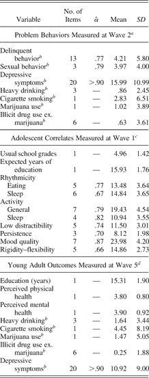
Delinquent behaviors were measured using 13 items selected from prior delinquency research (Elliott, Huizinga, & Menard, Reference Elliott, Huizinga and Menard1989). Thirteen items measured delinquent behavior encompassing property damage (e.g., destroyed school or other public property), aggression (e.g., beat up someone on purpose), and theft (e.g., stole from a store something valued at $20 or less). Three items measured sexual behavior (e.g., engaged in sexual activity not involving actual intercourse, engaged in sexual activity involving actual intercourse, and the number of different persons a participant has had intercourse with). Adolescents were asked to indicate the number of times they were involved in each of the 16 behaviors during the last 6 months prior to assessment. Response options were coded: 0 = never, 1 = once, 2 = 2–3 times, 3 = 4–5 times, 4 = 6–9 times, 5 = 10 or more. Scores from individual items were summed to create two scale scores for delinquent behavior and sexual behavior. The internal consistency measures for the delinquent and sexual behaviors were .77, and .79, respectively. Means, standard deviations, and internal consistency estimates of all measures used in this study are shown in Table 1.
Descriptive statistics of the variables measured at three time points in adolescence and young adulthood

aAverage age = 16.0 years.
bReported values are in original scale units; these variables were log-transformed in subsequent analyses.
cAverage age = 15.5 years.
dAverage age = 24.2 years.
Heavy drinking, smoking, and other substance use
Participants were asked how many times they drank six or more cans or bottles of beer, glasses of wine, or drinks of liquor at one time during the last 6 months (heavy drinking). The three responses for the different alcoholic beverages were summed and divided to create a composite score of heavy drinking that reflected the average number of times participants engaged in heavy drinking per month over the past 6 months. Cigarette smoking was assessed using the average quantity that individuals smoked per day during the last 6 months with a seven-option response format: None, less than 1 cigarette per day, 1–5 cigarettes per day, about one-half pack per day, about 1 pack per day, and about 2 packs or more per day. The measures of marijuana use and other illicit drug use (e.g., cocaine, stimulants, barbiturates, hallucinogens) assessed how often participants had used these substances during the previous 6 months (frequency). The response options were never, a few times in past 6 months, about once a month, 2–3 days a month, about once a week, 2–3 days a week, 4–5 days a week, and every day. The validity of adolescent self-reports of cigarette smoking (e.g., Wills & Cleary, Reference Wills and Cleary1997), drinking and other substance use (e.g., Winters, Stinchfield, Henly, & Schwartz, Reference Winters, Stinchfield, Henly and Schwartz1991) has been supported in existing research studies.
Depressive symptoms
Depressive symptoms were assessed using the Center for Epidemiologic Studies Depression Scale (CES-D; Radloff, Reference Radloff1977). The CES-D consists of 20 self-report items and provides a unitary measure of current depressive symptomatology, with an emphasis on the affective component, depressed mood. Participants are asked to indicate how many days during the past week they experienced the emotions or behaviors indicated in each of the items. The response options for these items ranged from 0 = rarely or none of the time to 3 = most or all of the time.
Adolescent correlates measured at Wave 1
Temperament
The Revised Dimensions of Temperament Survey (DOTS-R) was used to assess adolescent temperament at Wave 1 (Windle, Reference Windle1992; Windle & Lerner, Reference Windle and Lerner1986). The DOTS-R is a 54-item self-report measure that assesses 10 temperament attributes. A four-choice response format was used for each item, with responses ranging from 1 = usually false to 4 = usually true. Concurrent and predictive validity for the DOTS-R have been documented in previous studies (see Windle, Reference Windle1992). Higher subscale scores indicate higher levels of that temperamental characteristic. Of the 10 temperament attributes, the following eight scales were used in the study: rhythmicity-sleep (regularity of sleeping habits in timing and amount), rhythmicity-eating (regularity of eating habits in timing and amount), activity level-general (overt motor activity, energy, getting fidgety), activity level-sleep (tossing and turning in bed), low distractibility (concentrating and maintaining perceptual focus despite distractions), persistence (continuing in an activity for a relatively long period of time), mood quality (levels of positive affect—smiling and being cheerful), and rigidity–flexibility (responding to changes in environment).
Usual grades in school and years of education expected to complete
Adolescents were asked at Wave 1 what grades they usually got in school. Responses ranged from 1 = mostly Ds and Fs to 6 = mostly As. A higher score reflected better grades. The correlation between adolescents' reports of their GPA and official high-school records (that used a somewhat different measurement scale) was .78. Therefore, this self-report item was judged as valid. Dornbusch, Mont-Reynaud, Ritter, Chen, and Steinberg (Reference Dornbusch, Mont-Reynaud, Ritter, Chen, Steinberg, Colten and Gore1991) reported a similar correlation (r = .79) with a sample of 5,000 students. Adolescents were also asked how many years of education they thought they would complete in their lifetime.
Young adult outcome variables measured at Wave 5
Years of education completed, and perceived physical and mental health
Young adults reported on the number of years of education that they had completed. For physical and mental health, young adults were asked two questions: “How would you rate your overall physical health?” and “How would you rate your overall mental or emotional health?” Response options ranged from 1 to 5: 1 = poor, 2 = fair, 3 = good, 4 = very good, and 5 = excellent.
Heavy drinking, smoking, and other substance use
The items assessing heavy drinking, smoking, and other substance use in young adulthood were the same as those used in adolescence.
Psychiatric and substance abuse disorders
Positive lifetime and 12-month psychiatric diagnoses of alcohol use disorder (AUD), cannabis use disorder (CUD), and major depressive disorder (MDD) were derived in the young adulthood interview via the World Health Organisation (WHO) Composite International Diagnostic Interview (WHO, 1997) based on the DSM-IV criteria (American Psychological Association, 1994). The prevalence rates of these disorders in our sample are similar to those reported in the National Cormorbidity Study (NCS; Kessler et al., Reference Kessler, McGonagle, Zhao, Nelson, Hughes and Eshleman1994; for more information see Windle & Wiesner, Reference Windle and Wiesner2004).
Results
Model-based cluster analysis: Identification of groups
The total sample of 1,126 participants had a very small fraction of the data missing (less than 0.1%) on the seven problem behavior variables. The EM algorithm for ML was used for imputation using the SPSS Missing Value Analysis (SPSS, 1989–2004). Little's Missing Completely at Random Test (MCAR; Little, Reference Little1988) resulted in nonsignificant, χ2 (df = 22) = 30.194, p = .114, thus indicating random missing values and subsequent unbiased imputation of missing values. The seven problem behaviors were log-transformed to normalize skewed distributions using the natural logarithm after adding a constant of one. Data were assessed for the degree to which the data fit multivariate normal distributions both before and after subjecting them to data transformations. Although model-based clustering methods work best when the data follow the multivariate normal distribution, the model-based clustering methods are reasonably robust to deviations from the multivariate normal distribution (Hardin & Rocke, 2004; Yeung et al., Reference Yeung, Fraley, Murua, Raftery and Ruzzo2001).
The log-transformed variables were then centered for males and females separately to account for a priori known gender differences in the means of these behaviors. This procedure takes into account any known gender differences in the level of these behaviors a priori so that derived cluster membership probabilities would mostly reflect individual differences or relative standings within, but not across, the same gender. If males and females differ only in terms of mean levels, the results would be equivalent to separate analyses for males and females (Venables & Ripley, Reference Venables and Ripley2002, p. 308). The results of the model-based cluster analysis are shown in Figure 1. The best fitting model involved a four-cluster solution BIC = −2,828.181. The best model consisted of four clusters of different volumes and shapes. The mixing proportion was .183 (n = 204), .235 (n = 265), .350 (n = 394), and .232 (n = 263) in the order of Clusters 1–4. The average posterior probabilities for the most likely cluster classification were .996, .989 .994, and .993, respectively, for Clusters 1–4 (see Appendices B and C for more information). This indicates a high degree of classificatory certainty for the four cluster solution.
We observed that the same model did not converge for five and more clusters. We relaxed the default tolerance level for the purpose of evaluating alternate cluster solutions (see Appendix C). The five-cluster model converged with the relaxed tolerance level and yielded a substantially better BIC, −2,362.02, with the mixing proportion .177 (n = 198), .144 (n = 156), .099 (n = 116), .347 (n = 393), and .232 (n = 263) in the order of Clusters 1–5. We statistically compared the overlap, or the lack thereof, between the two clustering solutions (i.e., the four- and five-cluster solutions) using the variation of information (VI) criterion proposed by Meilă (Reference Meilă, Schölkopf and Warmuth2003, 2007), which measures the amount of information lost in changing from clustering “a” to clustering “b,” and vice versa. This measure has a lower limit of 0 and an upper limit of 1, and is symmetric. The VI criterion, based on information theory, quantifies the amount of the conditional entropy not shared by the mutual information between the clusterings “a” and “b.” It is conceptually analogous to 1 – R 2 in analysis of variance or regression. Unlike Cohen's kappa, this statistic does not require that two clusterings have the same number of categories, nor is it necessary that two clusterings are ordered. The comparison of two clustering solutions yielded a value of .031, a relatively small value for the amount of information lost in comparing the four- and five-cluster solutions. Subsequently, we deemed the five cluster solution as a case of overextraction of components or overfitting, especially given that we greatly relaxed the tolerance level for relative convergence. A common pitfall associated with mixture models is that spurious maxima can be achieved that border on singularities for small but tightly clustered sets of data points (Hipp & Bauer, Reference Hipp and Bauer2006; Leisch, Reference Leisch2004; McLachlan & Chang, Reference McLachlan and Chang2004; McLachlan & Peel, Reference McLachlan and Peel2000). If a component (a cluster or class) is near empty, or two or more components have the same parameters, then it is generally considered as a red flag for the existence of a spurious cluster. One can counter the potential problem of finding a solution based on local optima by using different starting values (Hipp & Bauer, Reference Hipp and Bauer2006; Steinley, Reference Steinley2003), or by dividing a sample into random subsamples (McLachlan & Chang, Reference McLachlan and Chang2004).
For the purpose of validation, we randomly selected half of the sample with a selection probability = 0.5 and ran the same mixture model-based cluster analysis for 563 individuals. The same clustering model (diagonal, unequal volumes, and shapes) with four clusters was the best model, resulting in BIC = −1,889.229. The overlap between the full sample and the random half sample was substantial as indicated by the VI criterion = .085, and Cohen κ = .844, asymptotic standard error = .018, t = 34.532, p < .05. A Cohen κ exceeding .8 is widely considered as excellent chance-corrected agreement (von Eye & Mun, Reference von Eye and Mun2005, pp. 5–6). In addition, we divided the sample into four subsamples of an equal sample size (n = 281 or 282) and ran separate cluster analyses. Three or four clusters of the same clustering model (diagonal, unequal volumes, and shapes) were identified. When compared against the full sample, the VI criterion statistics showed evidence of small discrepancy, ranging from .052 to .166. In addition, we also took steps to evaluate that multivariate normality was observed in each cluster by examining the marginal distributions (univariate normality), and also by examining variance for univariate data and generalized variance for multivariate data. Based on the additional validation analyses involving subsamples of different sizes, we deemed the four cluster solution satisfactory.
Model-based cluster analysis: Interpretation of groups
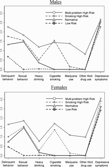
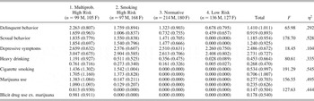
The four clusters included a multiproblem high-risk group (Cluster 1, n = 204; 99 males, 105 females) characterized by the highest levels of all problem behaviors, including high levels of multiple substance use including marijuana and other illicit substances; a smoking high-risk group (Cluster 2, n = 265; 97 males, 168 females) characterized by high levels of delinquent behavior, cigarette smoking, marijuana use, and depressive symptoms, and moderate levels of heavy drinking and sexual behavior; a normative group (Cluster 3, n = 394; 214 males, 180 females) characterized by overall low levels of delinquent and sexual behaviors, depressive symptoms, and heavy drinking; and a low-risk group (Cluster 4, n = 263; 136 males, 127 females) that showed almost nonexistent or very low levels of problem behaviors. The descriptive statistics of the seven behaviors for the four cluster groups are shown in Table 2 for males and females. The profile plots of seven problem behaviors for males and females are shown in Figure 2. Males and females were unequally represented across the four cluster groups, χ2 = 21.43, df = 3, p < .05. Configural frequency analysis (CFA; von Eye, Reference von Eye2002) showed that the data deviated substantially from the assumption of independence (i.e., equal representation of males and females in each cluster) in the following two cluster groups: males were more represented in the Normative group (Cluster 3; 54.3% males) and females were more highly represented in the smoking high-risk group (Cluster 2; 63.4% females) than expected by a model of proportional representation.
Profile plots of adolescent problem behaviors by cluster groups. The figure illustrates Table 2 in visually, so that the numbers along the y axis represent the averages of the log-transformed values reported in Table 2. [A color version of this figure can be viewed online at www.journals.cambridge.org]

Descriptive statistics of adolescent problem behaviors measured at Wave 2 (mean age = 16) by cluster groups (N = 1,126)
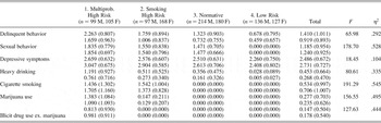
Note: The values, which are means (standard deviations), are averages of log-transformed values using the natural logarithm after adding a constant of 1. The top and bottom values in each pair are for males and females, respectively. See Figure 2 for a graphic illustration of this table.
Adolescent temperamental correlates
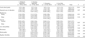
We analyzed how the cluster groups were different across measures of their usual school grades, educational expectations, and the temperamental characteristics assessed at Wave 1. Approximately 19% of the observations were missing for adolescent temperamental and educational variables at Wave 1. We conducted Little's MCAR test (Little, Reference Little1988), resulting in nonsignificant χ2 (df = 74) = 80.316, p = .288. We used the EM algorithm for ML for imputation of the missing values. We included cluster membership, gender, and their interaction as sources of variation (see Table 3). In terms of usual school grades, all three other cluster groups reported lower usual school grades than the low-risk group. The multiproblem high-risk and the smoking high-risk expected to complete fewer years of education than the low risk. Temperamental characteristics were also different across the four cluster groups. The multiproblem high risk and the smoking high risk reported lower levels of rhythmicity in eating and sleeping habits, were more distractible, and less persistent, and reported higher levels of activity compared to the low risk. The multiproblem high risk, however, was less flexible and more active in general activities than the smoking high risk. The Normative was, by and large, similar to the low risk in terms of temperamental characteristics with a few exceptions. The normative was more active and distractible. In addition to group differences because of cluster membership, females reported higher levels of usual school grades and positive mood quality, lower levels of rhythmicity, and were more distractible and less persistent.
Adolescent temperamental correlates at Wave 1 (mean age = 15.5) by cluster groups (N = 1,126)
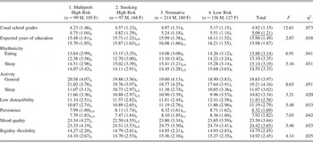
Note: Of the two rows of pairs of means (standard deviations), the numbers on the top and the bottom indicate mean values for males and females, respectively. Values with the same subscript are not significantly different from each other based on Tukey B post hoc tests. Underlined total means indicate significant gender differences. Interaction effects between cluster membership and gender on rhythmicity sleeping and mood quality were statistically significant. All F statistic values are significant at α ≤ .05.
Young adult follow-up
Of the 1,126 adolescents included in the model-based cluster analysis, we subsequently analyzed the 762 young adults who were retained at the Wave 5 follow-up.Footnote 2 The cluster membership information derived using data from Wave 2 and their continued participation in Wave 5 data collection were not independent, χ2 (3) = 9.25, p < .05. The nonparticipation rate was higher for the multiproblem high-risk group (40.7% vs. 28.7, 32.5, and 29.3% compared to the other cluster groups). Individuals who did not participate in the young adult assessment reported higher levels of involvement in delinquent behavior, means = 1.27 versus 1.11, F (df = 1124) = 6.53, p < .05; sexual behavior, means = 1.32 versus 1.16, F (df = 1124) = 7.57, p < .05; cigarette smoking, means = 0.71 versus 0.58, F (df = 1124) = 3.94, p < .05; and marijuana use, means = 0.31 versus 0.27, F (df = 1124) = 4.25, p < .05 among adolescent measures. Therefore, the subsequent findings in young adulthood should be interpreted along with these differential attrition rates that negatively affect the association between cluster membership and young adult variables.
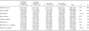
We compared the four groups on the number of years of completed education, overall perceived physical and mental health, depressive symptoms, heavy drinking, cigarette smoking, marijuana use, and other illicit drug use (Table 4). We used cluster membership, gender, and their interaction as explanatory terms in the model. The cluster membership derived at age 16 significantly predicted young adult outcome variables. The clusters had different mean locations in the years of education completed, overall physical health, heavy drinking, cigarette smoking, marijuana use, and illicit drug use (excluding marijuana use). In addition, there were gender differences for heavy drinking, marijuana use, and years of education completed, such that males reported higher levels of heavy drinking and marijuana use than females, and females reported completing more years of education. Interaction effects existed between gender and the cluster membership for heavy drinking and marijuana use.
Young adult follow-up measures at Wave 5 (mean age = 24.2) by cluster groups (N = 762)

Note: The values are means (standard deviations). The top and bottom values in each pair are for males and females, respectively. Reported values of heavy drinking, cigarette smoking, marijuana use, illicit drug use, and depressive symptoms are averages of log-transformed values using the natural logarithm after adding a constant of 1. Values with the same subscript are not significantly different from each other based on Tukey B post hoc tests. Underlined total means indicate significant gender differences. The interaction effects between cluster membership and gender on heavy drinking and marijuana use were statistically significant. All F statistic values are significant at α ≤ .05 unless noted otherwise.
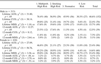
Young adult substance use disorder by cluster groups (N = 723)
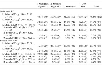
Note: AUD, alcohol use disorder; CUD, cannabis use disorder; MDD, major depressive disorder. Percentages are the proportions of cases meeting criteria for a diagnosis within each of the cluster groups. The numbers in parentheses indicate the actual number of case criteria for a diagnosis within each of the cluster groups.
Overall, the multiproblem high risk showed poor developmental profiles as young adults as indicated by highest levels of heavy drinking, marijuana use, and other illicit drug use. The multiproblem high risk also reported lower levels of educational attainment and physical health; the smoking high risk was statistically not distinguished from the multiproblem high risk on the domains of years of completed education, perceived physical health, and cigarette smoking, but significantly separated from the multiproblem high risk on heavy drinking, marijuana use, and illicit drug use. Compared to the normative who reported elevated levels of heavy drinking and marijuana use in young adulthood, the smoking high risk had lower levels of education and higher levels of cigarette smoking. The normative was, by and large, similar to the low-risk group with two exceptions of moderate levels of marijuana use and heavy drinking.
Lifetime and 12-month substance use and MDD diagnoses
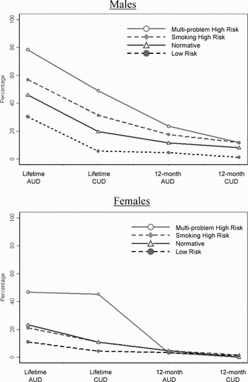
Lifetime and 12-month substance use disorder and MDD diagnoses were made for 313 males and 410 females of the 762 participants at Wave 5. Chi-square analysis showed that lifetime AUD and CUD were significantly associated with the cluster membership for males and females (see Table 5 and Figure 3). The multiproblem high risk, in particular, had 78.4 and 46.8% of males and females, respectively, who met criteria for a lifetime AUD diagnosis. The multiproblem high risk also showed 49.0 and 45.2% of males and females, respectively, who met criteria for a lifetime CUD diagnosis. The AUD and CUD diagnoses for the past 12 months were statistically associated with cluster group membership only for males. For males, the multiproblem high risk had 23.5 and 11.8% of the individuals meeting criteria for the 12-month AUD and CUD diagnoses, respectively. The AUD and CUD diagnoses for the past 12 months were not associated with cluster group membership for females. The lifetime and 12-month MDD diagnoses were not associated with cluster membership for males or females.
Lifetime and 12-month alcohol use disorder and cannabis use disorder diagnoses by cluster groups in young adulthood. [A color version of this figure can be viewed online at www.journals.cambridge.org]

Discussion
Model-based cluster analysis
The current study sought to examine the heterogeneity of problem behaviors among adolescents using a mixture model-based cluster analysis approach. This new analytical procedure is a tool to empirically investigate population heterogeneity and accordingly to classify subpopulations using more rigorous statistical methods for the comparison of alternative models. Model-based cluster analysis utilizing finite mixture densities can be a valuable analytic tool for research on developmental psychopathology for a number of reasons. First, model-based cluster analysis can be used to generate a new set of hypotheses based on detected salient patterns of cases or individuals. Because developmental psychopathology is an integrative discipline that often faces unique challenges to synergize emerging cross-area information (e.g., genetics, neuroscience, psychology, sociology, epidemiology) as they become available to better understand the mechanisms through which psychopathology develops (Cicchetti & Rogosch, Reference Cicchetti and Rogosch2002), it often becomes necessary for researchers to explore data to generate new hypotheses for future directions. Second, this method can be used in comparing subgroups when measurement invariance across subpopulations cannot be established. Measurement invariance is defined as the measurement model that relates the observed variables to the underlying factors is identical across subpopulations and requires equality of factor loadings, intercepts, and residual variances across subpopulations (Meredith, Reference Meredith1993). Model-based cluster analysis does not require the assumption of measurement invariance across different populations, and may be used as an alternative method when the assumption of measurement invariance is either untenable or unreasonable. Third, a model-based cluster analysis can be used to address person-oriented questions that have arisen through variable-oriented research. For example, the literature on child maltreatment suggests that of the three types of often co-occurring maltreatment (i.e., emotional maltreatment, physical neglect and abuse, and sexual abuse), only emotional maltreatment predicted slower increases in self-esteem and slower decreases in depressive symptoms over time for 7- to 12-year-olds when initial levels of depressive symptoms, age, and the other types of maltreatment were controlled (Kim & Cicchetti, Reference Kim and Cicchetti2006). One important follow-up task may be to empirically find the group of children meeting the aggregate-level prediction and other groups of children who do not, and to then investigate their biological, psychological, and environmental characteristics that guided them toward divergent paths.
In the present study we identified four clusters of adolescents who varied with regard to their specific risk behaviors and levels of seven problem behaviors, and we found that the four clusters of adolescents differed significantly from one another on a number of adolescent temperamental characteristics and across young adult outcome measures. The results demonstrate the utility of a model-based cluster analysis as an improved alternative method to heuristic cluster analytic procedures when finding heterogeneous groups in a population. However, it is important to note that any classification should pass the tests of not only statistical validity but the usefulness or meaningfulness of the derived clusters (Everitt et al., Reference Everitt, Landau and Leese2001; Muthén, Reference Muthén2003; Rindskopf, Reference Rindskopf2003; von Eye & Bergman, Reference von Eye and Bergman2003). Citing a point made by Needham (Reference Needham and Hymes1965) regarding the classification of humans into men and women and its usefulness as a classification because it carries more information than mere anatomical differences, Everitt and colleagues (Reference Everitt, Landau and Leese2001, p. 4) illustrated this point using an analogy of classifying books:
A similar point can be made in respect of the classification of books based on subject matter and their classification based on the color of the book's binding. The former, with classes such as dictionaries, novels, biographies, etc., will be of far wider use than the latter with classes such as green, blue, red, etc. The reason why the first is more useful than the second is clear; the subject matter classification indicates more of a book's characteristics than the latter. So it should be remembered that in general a classification of a set of objects is not like a scientific theory and should be judged largely on its usefulness, rather than in terms of whether it is “true” or “false” [italics added].
Therefore, results from cluster analyses should be evaluated not only by the ways that objects are classified but also with regard to the generality or usefulness of the clusters for subsequent use, which, in the present study, demonstrated predictive utility for young adult outcome measures.
Four clusters and their profiles
Substantively, we identified four clusters based on the problem behaviors of delinquent behaviors, sexual behavior, substance use, and depressive symptoms in adolescence. Examining clusters of individuals based on multiple problem behaviors enabled us to find distinctive cluster profiles of adolescents. As indicated by profile plots, illicit drug use at age 16 appears to be a good proxy of risk for a constellation of problem behaviors, including delinquent and violent behaviors for a normative community-based sample. The multiproblem high-risk group accounted for 18.3% of the total sample and exhibited the highest levels of other concurrent problem behaviors measured in this study, including delinquent behavior, other substance use (e.g., cigarette smoking, marijuana use, heavy drinking), and depressive symptoms, and reported lower school grades. Temperamentally, the multiproblem high-risk group was more irregular in terms of eating and sleeping habits, more rigid and distractible to changes in the environment, more active, less persistent in pursuing tasks, and had poor mood quality, compared to the low risk in adolescence. Individuals of this high-risk group had lower levels of usual school grades, educational expectations for themselves in adolescence, and subsequently completed fewer years of education by young adulthood. They also reported poor overall physical health, and continued involvement in heavy drinking, cigarette smoking, marijuana use, and other illicit drug use in young adulthood. The multiproblem high risk also featured elevated proportions of cases meeting diagnostic criteria for lifetime AUD and CUD for both males and females. High proportions of males in this cluster group also met criteria for the 12-month AUD and CUD diagnoses.
The smoking high-risk group accounted for 23.5% of the total sample. The smoking high risk manifested high levels of cigarette smoking, marijuana use, and depressive symptoms in adolescence. Temperamentally and academically, they closely mirrored the profiles of the highest risk group. Compared to the low risk, they were more irregular and hyperactive, more distractible, and less persistent in their self-reported temperament and, as expected, had lower levels of usual school grades, and educational expectations for themselves in adolescence and subsequently completed fewer years of education by young adulthood. Although these individuals also maintained involvement in heavy drinking, cigarette smoking, and marijuana use in young adulthood, the smoking high-risk groups reported lower levels of heavy drinking, marijuana use, and other illicit drug use in young adulthood than the multiproblem high risk. The normative and the low-risk groups accounted for 35.0 and 23.2% of the total sample, respectively. Although the normative engaged in moderate levels of delinquent and sexual behaviors, and heavy drinking, they were largely inseparable from the low risk in terms of their temperamental and educational attributes in adolescence. However, there was evidence that some individuals of the normative, compared to the low risk, showed involvement in marijuana use and heavy drinking episodes in young adulthood, which may be interpreted as occasional substance use in social settings for this subset of individuals.
The continuity and comorbidity path from middle adolescence to young adulthood
The transitional period from adolescence to emerging young adulthood is “a window of opportunity for changing the life course” in terms of having second-chance opportunities or experiencing a turning point (Masten et al., Reference Masten, Burt, Roisman, Obradovic, Long and Tellegen2004). Adult roles can alter one's own expectations and circumstances, thus eliciting encouraging changes (i.e., “adult-role socialization”). It is known that marriage itself is associated with reduced alcohol use (Miller-Tutzauer, Leonard, & Windle, Reference Miller-Tutzauer, Leonard and Windle1991) and with reduced crime (Sampson, Laub, & Wimer, Reference Sampson, Laub and Wimer2006). However, the current study showed that there is also remarkable continuity of risk and dysfunction from adolescence to young adulthood. The current findings suggest that a majority of problem or risk behaviors are carried out by a small group of adolescents (multiproblem high risk, 18.3%) who use hard drugs by age 16 and that these adolescents are more deeply entrenched of the two high risk groups toward the addictive life path as the gateway theory suggests (Kandel, Reference Kandel1975; Newcomb & Bentler, Reference Newcomb and Bentler1988), and illicit drug use by age 16 appears to be a good proxy of risk for other problem behaviors.
The gateway theory of substance use suggests that there is an orderly stagelike progressive sequence of substance use that adolescents go through starting with legal substances such as tobacco or alcohol and proceeding to illicit hard drugs such as marijuana and cocaine, and that the orderly sequence is hard to reverse or to deviate from once initiated as if walking through a “tunnel” (Kandel, Reference Kandel and Kandel2002). Although this is a rigid picture, it may be best understood in the context of recent studies that early entry into substance use such as heavy alcohol use, in and of itself, is shown to damage the prefrontal cortex, which is critical for executive functions such as impulse control and goal setting in animal models, and to lead to impaired cognitive functioning in human adolescents (Monti et al., Reference Monti, Miranda, Nixon, Sher, Swartzwelder and Tapert2005; Reyna & Farley, Reference Reyna and Farley2006). Therefore, it is plausible, for instance, that adolescents who initiate heavy drinking at an earlier age would be vulnerable for other risk behaviors because their decision-making ability to avoid them is compromised in ways that are stable across time and situations in addition to acute, erratic, risky decisions because of acute alcohol consumption.
The current findings are consistent with other studies on the age of onset as an indicator of risk that have suggested that ages 12–15 as a sensitive time window in development for initiation of a range of problem behaviors for at-risk individuals (e.g., age 12 for any substance use; Kaplow, Curran, Dodge, & the Conduct Problems Research Group, 2002; and age 15 for sexual intercourse; Capaldi, Stoolmiller, Clark, & Owen, Reference Capaldi, Stoolmiller, Clark and Owen2002; Raffaelli & Crockett, Reference Raffaelli and Crockett2003). Current findings of illicit drug use at age 16 as a proxy of serious risks suggest that in early teen years coinciding with the advent of puberty, some adolescents initiate risk behaviors beginning with tobacco and alcohol use, then rapidly progress toward other problem behaviors of greater potential harms, and expand their inventory of problem behaviors by middle adolescence. In addition, once adolescents are on the risky path, they are more likely to have to tackle behavioral and social consequences of being arrested and questioned by police, or being suspended from school in adolescence.
In sum, the continuity and comorbidity path from middle adolescence to young adulthood may progress through a sequence of risk aggregation. First, some adolescents appear not to be on equal footing with others when facing risk behaviors as indicated by adolescent risky temperamental characteristics. For example, adolescents who are more active during sleep (low risk vs. all others) could be an indication of sleep problems that are increasingly linked to adjustment problems in childhood and adolescence, including early onset of alcohol and other drug use (Wong, Brower, Fitzgerald, & Zucker, Reference Wong, Brower, Fitzgerald and Zucker2004), and neurobehavioral functioning and behavior problems (Sadeh, Gruber, & Raviv, Reference Sadeh, Gruber and Raviv2002), although the exact mechanisms of these associations remain unknown. Second, adolescents with early onset of multiple substance use and sustained use may become even more vulnerable by their own use. At a time period when the adolescent brain continues to develop well into the mid-20s, especially in the frontal lobes critical for executive functions such as impulse control, substance-abusing adolescents may be sabotaging their own chances in life by putting themselves at even higher risk for other risk behaviors that require better judgment and decision-making to avoid escalating, multiple problems. Thus, the maladaptive patterns of behavioral and emotional self-regulation, and reactivity to the demands of the surrounding environment, become more entrenched. Third, as at-risk adolescents develop, they may be more active in constructing their niche with others with similar attributes, values, and behaviors (e.g., selection of deviant peers), thereby the interlocking continuity gets reinforced as they transition into young adulthood. From a prevention science perspective, the current study underscores the importance of providing early intervention that is tailored for potentially variable needs of different adolescents. Empirically identifying adolescents at risk via sound methods would provide initial steps for understanding and devising ways to intervene and gauging the intensity of the intervention needed.
Limitations and Future Directions
The present study has several limitations. First, the sample for this study was geographically and ethnically limited. Although the schools selected were public schools, the majority of the participants were Catholic, European American, and all participants resided in Western New York at the initial assessment. The sample in this study represents a normative, community-based adolescent sample that includes some high-risk but also low-risk adolescents. Thus, the cluster findings should be generalized to normative adolescent populations; however, they cannot be generalized to high-risk or at-risk populations such as juvenile delinquents. In addition, the current sample was drawn from a few primary sampling units (schools) within which adolescents were nested. This nested data structure typically results in biased standard errors. The exact degree of the bias is unknown, and the study results should be interpreted cautiously because of its homogeneous data characteristics. Second, we relied on self-reports by adolescents to assess their problem behaviors. Although self-reported measures of problem behaviors are widely used in the literature and the validity of those measures have been shown (e.g., smoking measure; Wills & Cleary, Reference Wills and Cleary1997, substance use; Winters et al., Reference Winters, Stinchfield, Henly and Schwartz1991), the extent to which these problem behaviors are correlated because of shared methods is unclear. Third, the present study did not exhaustively include all domains of interest in young adulthood and was limited to young adult outcomes of years of completed education, overall perceived mental and physical health, substance use, and substance use disorders. One obvious area not covered in this study was risky sexual behavior for all participants and reproductive health for females as one of the young adult outcomes, which has been suggested to be related to drinking and substance use in women (see Wilsnack, Plaud, Wilsnack, & Klassen, Reference Wilsnack, Plaud, Wilsnack, Klassen, Wilsnack and Wilsnack1997). In addition, the sexual behavior measured at age 16 mostly likely reflected initiation of sexual activities rather than persistently higher risky sexual behavior (e.g., unprotected sex with multiple partners). For this reason, we suspect that sexual behavior at age 16 was not uniquely related to adolescent and young adult measures included in the present study. For example, the normative did not differ from the low risk in almost all measures. Consistent with data from a national sample of 11th graders, which indicated that 53.2% of adolescents have experienced sexual intercourse (Grunbaum et al., Reference Grunbaum, Kann, Kinchen, Ross, Hawkins and Lowry2004), sexual initiation by age 16 may not be a good measure of generalized problem or risky behaviors. In addition, previous studies have shown that risk factors such as self-regulation may be associated more with risky sexual behavior rather than with the initiation of sexual activity (Raffaelli & Crockett, Reference Raffaelli and Crockett2003). We also did not assess tobacco dependence at Wave 5, which would be of great interest, especially for the smoking high-risk group.
Despite these limitations, we believe that the current study has strengths and contributes to the literature. First, this study utilized a large sample of adolescents and found four distinctive clusters of adolescents that differed not only in their risk level but also in their risk kind. Many existing studies have focused primarily on the unique effects of one variable (e.g., cigarette smoking) above and beyond the effects of other predictors (e.g., heavy drinking). This approach does not address the issue of co-occurring problem behaviors at the individual level. In other recent studies that have used latent growth analysis, the analytic focus has most often been on one problem behavior at a time, thereby preventing the opportunity to understand the common and unique etiological processes of multiple behavior problems underlying their expression (Chassin et al., Reference Chassin, Flora and King2004). The approach taken in this study allowed us to identify other at-risk profiles that may be relevant to understanding and promoting successful transitions to adulthood. Moreover, unlike many other existing clustering procedures, the new mixture clustering method used in this study adopts finite mixture densities and the maximum likelihood estimation method that is ideal for finding groups unknown in advance but where patterns are suspected. The model-based cluster analysis using MCLUST program (Fraley & Raftery, Reference Fraley and Raftery2002a, Reference Fraley and Raftery2002b, Reference Fraley and Raftery2003), in particular, eliminates the subjective arbitrariness one faces when selecting a clustering procedure and deciding the number of clusters, which is especially important because a trade-off generally exists between model complexity and the number of clusters (e.g., Bauer & Curran, Reference Bauer and Curran2003, Reference Bauer and Curran2004).
Second, the current study not only identified a high-risk cluster of adolescents and their adolescent correlates at age 15.5–16 years old, but also prospectively followed them into young adulthood when they were approximately 24.2 years old. Results indicated that in addition to the highest risk group of adolescents identified in adolescence (i.e., the multiproblem high-risk group), there were other individuals sharing the unique risk profile of problem behaviors. The smoking high-risk group, in particular, continued to participate in heavy drinking, cigarette smoking, and marijuana use as young adults, although it is unclear from the current study whether their risk is reduced only in levels, compared to the multiproblem high risk, because of a lack of diverse young adult measures. The findings in this study direct us to contemplate the importance of investigating aggregated problem behaviors from a within-person perspective in the course of adolescence and young adulthood. Third, this study included depressive symptoms and sexual behaviors, which are highly prevalent among females. Thus, we were able to derive clusters that may be more typical of a normative sample for both male and female adolescents. It is highly important to learn more about different subgroups of individuals that differ not only in their level of risk but also in the nature (e.g., developmental changes) of their risk so that we can understand common and unique causal mechanisms associated with being a member of different clusters, and ultimately contribute to the development of effectively tailored prevention and intervention programs based on this knowledge. New studies may gain from the approach taken in this study to find a mixture of clusters for developmental psychopathology research and to conduct follow-up studies with more ethnically and racially diverse samples and with a broader range of risk and protective factors, as well as outcomes.
Appendix A
A graphic illustration of volume, shape, and orientation in two-dimensional space. An example of Model A, spherical, equal volume, and equal shape in two-dimensional space. It was drawn using two normally distributed random variables (N = 200). The solid lines indicate spherical clusters and encircled dotted lines indicate orientation. [A color version of this figure can be viewed online at www.journals.cambridge.org]

An example of Model I is ellipsoidal, unequal volume, equal shape, and varying orientation in two-dimensional space. These data came from the classic Fisher's Iris data set featured in Everitt and Hand (Reference Everitt and Hand1981) and Fraley and Raftery (Reference Fraley and Raftery1998, Reference Fraley and Raftery1999, Reference Fraley and Raftery2002a, Reference Fraley and Raftery2002b, Reference Fraley and Raftery2003). Two ellipsoids are different in their respective volume and orientation. [A color version of this figure can be viewed online at www.journals.cambridge.org]

Appendix B: Geometric Properties of Covariance Matrix
Model-based clustering utilizes finite mixture models with the underlying idea that the observed data set is originated from a mixture of several subpopulations, and that the group membership is a priori unknown. Although the parametric densities can be various, multivariate normal densities are often used to model the components. The observed covariance matrix is decomposed into the following general form

where λk parameterizes the volume of the kth cluster, D k indicates the orientation of that cluster, and A k represents the shape of that cluster (Banfield & Raftery, Reference Banfield and Raftery1993, Fraley & Raftery, Reference Fraley and Raftery1998, Reference Fraley and Raftery1999, Reference Fraley and Raftery2002a, Reference Fraley and Raftery2002b, Reference Fraley and Raftery2003). The subscript k indicates that each component can have different volume, shape, and orientation. The 10 models tested simultaneously using the MCLUST software package reflect different spectral decompositions: A, spherical, equal volume, equal shape; B, spherical, unequal volume, equal shape; C, diagonal, equal volume, equal shape; D, diagonal, unequal volume, equal shape; E, diagonal, equal volume, varying shape; F, diagonal, unequal volume, varying shape; G, ellipsoidal, equal volume, equal shape, equal orientation; H, ellipsoidal, equal volume, equal shape, varying orientation; I, ellipsoidal, unequal volume, equal shape, varying orientation; J, ellipsoidal, unequal volume, varying shape, varying orientation.
Model A is the most simplistic model and Model J is the most complex model. Model A, in particular, has been shown to be very closely related to the k-means clustering algorithm (Celeux & Govaert, Reference Celeux and Govaert1992; Everitt et al., Reference Everitt, Landau and Leese2001; Yeung et al., Reference Yeung, Fraley, Murua, Raftery and Ruzzo2001). Note that a trade-off generally exists between the number of clusters and the number of estimated parameters in the sense that the more simplistic models may require a larger number of clusters to adequately fit the data, whereas a small number of clusters may be sufficient with increasingly more complex models to provide adequate fit to the data (Yeung et al., Reference Yeung, Fraley, Murua, Raftery and Ruzzo2001; for an empirical demonstration applied to, for instance, latent class growth trajectory analysis, see Bauer & Curran, Reference Bauer and Curran2003, Reference Bauer and Curran2004).