





1. Introduction
Evaporation of sessile colloidal droplets is a common phenomenon in both industrial processes and nature. Perhaps the most familiar example is the so-called ‘coffee-ring’ effect, in which the evaporation-driven thinning of a droplet with a pinned contact line drives an outward flow, transporting particles to the contact line where they accumulate to form an annular deposit (Deegan et al. Reference Deegan, Bakajin, Dupont, Huber, Nagel and Witten1997, Reference Deegan, Bakajin, Dupont, Huber, Nagel and Witten2000). The effect is ubiquitous for many different colloids and may be advantageously exploited in, for example, microscale colloidal patterning (Harris et al. Reference Harris, Hu, Conrad and Lewis2007), microcircuits (Layani et al. Reference Layani, Gruchko, Milo, Balberg, Azulay and Magdassi2009), DNA mapping (Blossey & Bosio Reference Blossey and Bosio2002) and blood spatter analysis (Smith & Brutin Reference Smith and Brutin2018), while being a drawback in situations where uniform particle deposition is required, for example in certain inkjet printing or additive manufacturing applications (He & Derby Reference He and Derby2017; Pahlavan et al. Reference Pahlavan, Yang, Bain and Stone2021).
Given its ubiquity and broad range of applications, the evaporation of sessile colloidal droplets has attracted sustained research interest over several decades, as summarized in numerous recent reviews (Sefiane Reference Sefiane2014; Brutin & Starov Reference Brutin and Starov2018; Parsa et al. Reference Parsa, Harmand and Sefiane2018; Lohse & Zhang Reference Lohse and Zhang2020; Parthasarathy et al. Reference Parthasarathy, Thampi, Ravindran and Basavaraj2021; Yang et al. Reference Yang, Jiang, Lyu, Ding and Man2021; Gelderblom et al. Reference Gelderblom, Diddens and Marin2022; Thampi & Basavaraj Reference Thampi and Basavaraj2023; Wilson & D’Ambrosio Reference Wilson and D’Ambrosio2023). One of the most important challenges is how to control the drying process in order to obtain the deposition profile that is most suited to a specific application (Mampallil & Eral Reference Mampallil and Eral2018). When the goal is to suppress the coffee-ring effect, techniques that inhibit pinning of the contact line such as using superhydrophobic (Dicuangco et al. Reference Dicuangco, Dash, Weibel and Garimella2014) or oil-covered (Li et al. Reference Li, Diddens, Segers, Wijshoff, Versluis and Lohse2020) substrates and electrowetting (Li & Mugele Reference Li and Mugele2008) are effective as they may lead to a more uniform profile. Similarly, surfactants may be used to drive Marangoni flows that counter the evaporation-driven liquid flow, inhibiting the outward transport of particles (Hu & Larson Reference Hu and Larson2006; Wang et al. Reference Wang, Karapetsas, Valluri and Inoue2024). Marangoni flows may also be driven by variation in the substrate temperature, leading to a large central deposit known as a ‘coffee eye’ (Li et al. Reference Li, Lv, Li, Quéré and Zheng2015) and also in situations where it is feasible to introduce another liquid to the mixture to form a binary droplet (see, for example, Kim et al. (Reference Kim, Boulogne, Um, Jacobi, Button and Stone2016) and Pahlavan et al. (Reference Pahlavan, Yang, Bain and Stone2021)), where the flow patterns may be significantly more complex and depend on various liquid properties, such as the relative volatility of the components.
In choosing how to control the phenomenon advantageously, it is critical to understand the complexities of the internal dynamics and how the coffee ring grows. The most widely studied models stem from the seminal work of Deegan et al. (Reference Deegan, Bakajin, Dupont, Huber, Nagel and Witten1997, Reference Deegan, Bakajin, Dupont, Huber, Nagel and Witten2000) and exploit the simplifications afforded by the following key modelling assumptions (see, for example, Gelderblom et al. (Reference Gelderblom, Diddens and Marin2022) and Wilson & D’Ambrosio (Reference Wilson and D’Ambrosio2023)). Firstly, they focus on thin, axisymmetric droplets, so as to simplify dramatically the geometry and evolution equations for the transport of liquid, particles and liquid vapour. Secondly, they focus on the diffusion-limited evaporative regime in which the diffusive transport of vapour away from the liquid–gas interface is rate-limiting, so that the evaporative flux has a particularly simple form that is inverse square-root singular at the contact line for a thin droplet. Thirdly, they focus on the low-volume-fraction regime in which the suspension of colloidal particles is initially dilute, so that both the finite size of the growing ring deposit and particle–fluid interactions can be neglected to a first approximation, the liquid advecting the particles towards the pinned contact line as the droplet thins. The tractability of the resulting ‘Deegan-style’ models facilitates not only the mechanistic insights in the original contribution, but the study of numerous additional effects, including the role of diffusive transport of the colloidal particles (Moore et al. Reference Moore, Vella and Oliver2021, Reference Moore, Vella and Oliver2022), gravity (Moore & Wray Reference Moore and Wray2023), substrate adsorption (Zigelman & Manor Reference Zigelman and Manor2018; D’Ambrosio et al. Reference D’Ambrosio, Wray and Wilson2025; Moore, D’Ambrosio & Wray Reference Moore, D’Ambrosio and Wray2025), contact angle (Hertaeg et al. Reference Hertaeg, Rees-Zimmerman, Tabor, Routh and Garnier2021), substrate morphology (D’Ambrosio et al. Reference D’Ambrosio, Colosimo, Duffy, Wilson, Yang, Bain and Walker2021) and droplet geometry (Sáenz et al. Reference Sáenz, Wray, Che, Matar, Valluri, Kim and Sefiane2017; Moore, Vella & Oliver Reference Moore, Vella and Oliver2022).
A particular aspect of the particle transport dynamics that is frequently overlooked is therefore the importance of finite volume fraction effects such as increased viscosity of the fluid mixture, particle jamming and the finite size of the ring deposit (Coombs et al. Reference Coombs, Chubynsky and Sprittles2024a ). The transport of colloidal particles towards the contact line drives the local volume fraction to increase until it reaches the critical jamming fraction – the time frame over which this occurs is typically rapid for diffusion-limited evaporation due to the singularity in the evaporation flux at the contact line (Moore et al. Reference Moore, Vella and Oliver2021). Even before jamming occurs, the Deegan-style decoupling of the flow and transport is likely to break down. However, many models that discuss particle transport and the final deposit profile neglect these effects entirely, despite the crucial role they play in the final shape and size of the deposit.
There are, however, notable exceptions. A natural approach is to relax the assumption that the liquid flow and particle transport may be decoupled by introducing a concentration-dependent viscosity and particle diffusion coefficient (Ozawa et al. Reference Ozawa, Nishitani and Doi2005; Yiantsios & Higgins Reference Yiantsios and Higgins2006; Eales et al. Reference Eales, Routh, Dartnell and Simon2015b ). In this manner, Kaplan & Mahadevan (Reference Kaplan and Mahadevan2015) derive a model in which the flow transitions from Stokesian and dilute in the bulk to essentially a plugged porous medium near the contact line, the latter region growing as the droplet dries. Similar ideas are applied in Coombs et al. (Reference Coombs, Chubynsky and Sprittles2024a , Reference Coombs, Sprittles and Chubynskyb ) and may also be used to treat drying polymers, where gelation near the contact line increases the local viscosity (Okuzono et al. Reference Okuzono, Kobayashi and Doi2009; Eales et al. Reference Eales, Dartnell, Goddard and Routh2015a , Reference Eales, Routh, Dartnell and Simonb ). However, one disadvantage of such approaches is that the constitutive relations for the viscosity and particle diffusion are typically prescribed empirically in terms of the particle concentration, for example by the Krieger–Dougherty law (Krieger & Dougherty Reference Krieger and Dougherty1959), and the resulting flow behaviour can depend strongly on the constitutive law chosen, which may itself depend on the liquid and the particles (Thiele Reference Thiele2014). Indeed, the constitutive law posed by Kaplan & Mahadevan (Reference Kaplan and Mahadevan2015) does not allow the mixture to completely jam before the liquid dries.
Deegan-style models have been shown in the several studies – see, for example, Wray et al. (Reference Wray, Wray, Duffy and Wilson2021), Wray & Moore (Reference Wray and Moore2023) and Wray & Moore (Reference Wray and Moore2024) – to predict with surprisingly high accuracy the net flux of particles delivered to, and hence the volume of, the ring deposit at the contact line, so that finite volume effects appear to be largely confined to a neighbourhood of the ring deposit. It therefore makes good modelling sense to consider in the first instance a model in which these effects are confined to the ring deposit in the dilute limit. Therefore, a simpler approach is to adopt a jamming model whereby in the bulk of the droplet, the particles are assumed to be passively transported by the liquid, while the coffee ring is modelled as a growing region of jammed particles at the contact line (Popov Reference Popov2005; Witten Reference Witten2009; Zheng Reference Zheng2009). The particles are assumed to take the particle jamming fraction in the ring, and the growth of the ring is modelled by a front that propagates into the droplet bulk from the contact line. This model has the distinct advantage that the liquid velocity is determined kinematically and coupled to the growth of the ring deposit by a simple system of differential equations. A similar approach has been used in gelating polymers (Okuzono et al. Reference Okuzono, Kobayashi and Doi2009) and in the context of desiccating blood droplets (Sobac & Brutin Reference Sobac and Brutin2014).
Despite the model of Popov (Reference Popov2005) being one of the simplest pertinent to coffee-ring deposition, it has not been the subject of the asymptotic analysis required to resolve systematically the non-uniformities that arise in the small-time, late-time and dilute limits. That such a delicate asymptotic structure arises is a consequence of the ring deposit growing in the neighbourhood of an initially pristine contact line at which the evaporative flux is singular and of the singularity that develops when the meniscus touches down on the substrate. A systematic asymptotic analysis is therefore crucial to the development of a tailored, high-precision scheme that is capable of bridging these limits, the predictions of the ensuing numerical simulations being used to validate the asymptotic predictions that underpin its development. Such a hybrid approach facilitates the extraction of novel mechanistic insight and the assessment of the veracity of the underlying modelling assumptions by comparing robust modelling predictions with experimental results.
The structure of the paper is as follows. In § 2, we reformulate the model of Popov (Reference Popov2005) and derive a reduced model, which we non-dimensionalize, contrast with that of the original and analyse qualitatively, before discussing the validity of the key modelling assumptions. In § 3, we present the results of our asymptotic and numerical analysis on a hierarchy of timescales up until touchdown of the meniscus, and compare the modelling predictions with a wide selection of experimental results. We conclude in § 4 with a summary of our results and a discussion of directions for future work.
2. Formulation and reduction of the mathematical model
2.1. Governing equations
In this section we revisit the formulation of the depth-averaged, kinematic model of Popov (Reference Popov2005) for evaporation-driven ring deposition in a thin, axisymmetric, colloidal droplet partially wetting an impermeable, rigid, planar substrate. The free boundary of the droplet is assumed to remain attached to the rim of a ring deposit that pins the contact line, as illustrated in figure 1. We introduce cylindrical polar coordinates
 $(r,z)$
with origin at the centre of the circular contact set of radius
 $a$
. We denote by
 $h(r,t)$
the droplet thickness and by
 $\phi (r,t)$
the volume fraction of colloidal particles, which are assumed to be spatially uniform in the cross-section. It is then self-consistent to assume that the deposit front at
 $r = s(t)$
is spatially uniform in the cross-section, splitting the droplet into the bulk region below the meniscus in
 $0 \lt z \lt h(r,t)$
for
 $0 \lt r \lt s(t)$
and the ring deposit in the region
 $0 \lt z \lt h(r,t)$
for
 $s(t) \lt r \lt a$
. The evaporation-driven thinning of the free boundary is assumed to drive an outward radial flow that transports the colloidal particles towards the contact line, just before which they are arrested instantaneously at the deposit front to form the rigid porous ring of jammed particles, through which the liquid may flow.
There is no flux of liquid through the substrate and the liquid is assumed to evaporate from the free boundary with an evaporative flux
 $E(r)$
that we shall prescribe shortly. There is no flux of particles through the substrate or free boundary. As described by Popov (Reference Popov2005) and Kaplan & Mahadevan (Reference Kaplan and Mahadevan2015), for example, the depth-averaged equations for conservation of liquid and colloidal particles are then given by
 \begin{align} \frac {\partial \ }{\partial t}\big (h(1-\phi ) \big ) + \frac {1}{r}\frac {\partial \ }{\partial r}\big (r h (1-\phi ) u_{l} \big ) = -E(r),\quad \frac {\partial \ }{\partial t}\big (h\phi \big ) + \frac {1}{r}\frac {\partial \ }{\partial r}\left (r h \phi u_{\kern-1pt p} \right ) = 0 \end{align}
in the bulk in
 $0 \lt r \lt s(t)$
and in the ring deposit in
 $s(t) \lt r \lt a$
, where
 $u_{l}(r,t)$
and
 $u_{\kern-1pt p}(r,t)$
are the depth-averaged radial velocities of the liquid and particles, respectively.
The colloidal particles are assumed to be advected with the liquid in the bulk of the droplet. The droplet is assumed to be sufficiently small that gravity may be neglected and the colloid–air interface to have a constant surface tension
 $\gamma$
, so that the free boundary forms a meniscus in the bulk whose thickness is governed by the thin-film version of the quasi-steady Young–Laplace equation with spatially uniform pressure
 $p_{0}(t)$
. Thus, the conservation of mass equations (2.1a
,
b
) are closed in the bulk by
 \begin{align} u_{\kern-1pt p} = u_{l},\qquad -\frac {\gamma }{r}\frac {\partial \ \ }{\partial r}\left (r\frac {\partial h}{\partial r}\right ) = p_{0} \quad \mbox{for} \quad 0 \lt r \lt s(t). \end{align}
The particles are assumed to be arrested instantaneously at the jamming volume fraction
 $\phi _{\textit{c}}$
at the deposit front, so that the conservation of mass equations (2.1a
,
b
) are closed in the ring deposit by
 \begin{align} \phi = \phi _{\textit{c}},\qquad u_{\kern-1pt p} = 0 \quad \mbox{for} \quad s(t) \lt r \lt a. \end{align}
Assuming that
 $s(t)$
decreases monotonically from its initial value of
 $a$
, there being no ring deposit initially, it follows from (2.1b
) and (2.3a
,
b
) that the thickness of the ring deposit ceases to evolve once it has been laid down, i.e.
 $\partial h/\partial t = 0$
for
 $s(t) \lt r \lt a$
. In our numerical simulations and comparisons with experimental data we shall use the value
 $\phi _{\textit{c}} = 0.64$
corresponding to that of randomly packed spheres. While the system would support the prescription of a jump discontinuity in
 $\phi _{\textit{c}}$
to model the ordered-to-disordered packing transition described by Marín et al. (Reference Marín, Gelderblom, Lohse and Snoeijer2011a
) for sufficiently small colloidal particles, we neglect such effects as in the model of Popov (Reference Popov2005).
Schematic of evaporation-driven ring formation in the depth-averaged kinematic model of Popov (Reference Popov2005), showing the evaporative flux of vapour (light-blue arrows), the bulk region below the meniscus (blue shading) and the rigid porous ring deposit (dark-blue shading).

Figure 1. Long description
A diagram of the evaporation-driven ring formation process in a colloidal droplet. The diagram shows the evaporative flux of vapour represented by light-blue arrows, the bulk region below the meniscus depicted with blue shading, and the rigid porous ring deposit shown with dark-blue shading. The diagram includes labels for the height of the droplet (h0(t)), the height of the ring deposit (hd(t)), the contact angle (θ(t)), the radius of the droplet base (a), the radius of the ring deposit (s(t)), and the volume of the ring deposit (vd(t)). The evaporative flux is directed upwards, while the flow within the droplet is directed horizontally towards the ring deposit. The diagram also includes mathematical expressions for the height of the droplet (z = h(r,t) = h0(t) − (p0(t)/4γ)r^2) and the flow velocity (u(r,t)).
The transport of the liquid vapour away from the droplet–air interface is assumed to be quasi-steady, dominated by diffusion and unhindered by the presence of the colloidal particles – the pores of the ring deposit remain saturated on the timescale of evaporation because the Darcy pressure drop required to supply the evaporative flux results in a pressure difference across the pore scale liquid–gas interface much smaller than the capillary entry pressure according to the estimates detailed in Routh & Russel (Reference Routh and Russel1998) and Coombs et al. (Reference Coombs, Chubynsky and Sprittles2024a ). In the thin-film limit the leading-order problem for the vapour concentration is equivalent to solving for the potential outside a charged disk in classical electrostatics (Sneddon Reference Sneddon1966; Deegan et al. Reference Deegan, Bakajin, Dupont, Huber, Nagel and Witten2000), the evaporative flux being given by
 \begin{equation} E(r) = \frac {2D_{l} M_{l} \Delta c}{\pi \rho _{l} \sqrt {a^2-r^2}}\quad \mbox{for} \quad 0 \lt r \lt a, \end{equation}
where
 $\rho _{l}$
,
 $D_{l}$
and
 $M_{l}$
are the density, diffusion coefficient and molar mass of the vapour, and
 $\Delta c$
is the difference between the saturation and ambient vapour concentrations.
We now impose the boundary and initial conditions that close the system (2.1)–(2.4), beginning with the symmetry conditions on the axis of symmetry that
 \begin{align} u_{l} = u_{\kern-1pt p} = 0,\qquad \frac {\partial h}{\partial r} = 0 \quad \mbox{at} \quad r = 0. \end{align}
At the deposit front, we assume that the droplet thickness, its partial derivatives and the liquid and particle flux (in the frame of the front) are all continuous, so that
 \begin{align} \Big [ h \Big ]_{-}^{+} = \bigg [ \frac {\partial h}{\partial t} \bigg ]_{-}^{+} = \bigg [ \frac {\partial h}{\partial r} \bigg ]_{-}^{+} = \Big [ r h(1-\phi ) \left (u_{l}-\dot {s}\right ) \Big ]_{-}^{+} = \Big [ r h \phi \left (u_{\kern-1pt p}-\dot {s}\right ) \Big ]_{-}^{+} = 0, \end{align}
where
 $[\boldsymbol{\cdot }]_{-}^{+}$
denotes the jump in a quantity across the deposit front at
 $r = {s}(t)$
whose outward radial velocity we denote by
 $\dot {{s}} = \mathrm{d}{s}/\mathrm{d} t$
. We note that in general
 $\phi$
,
 $u_{l}$
and
 $u_{\kern-1pt p}$
are discontinuous across the deposit front. The final boundary condition is that of no flux of liquid through the pinned contact line, which is given by
 \begin{equation} r h(1-\phi )u_{l} = 0 \quad \mbox{at} \quad r = a. \end{equation}
If the colloidal suspension is well mixed with volume fraction
 $\phi _{\star }$
when a droplet of volume
 $V_{\star }$
is seeded slowly onto the substrate, then it seems reasonable to impose the initial conditions
 \begin{align} \phi (r,0) = {\phi _{\star }} \,\mbox{ for }\, 0 \le r \lt s(0) = a,\quad h(a,0) = 0,\quad 2\pi \int _{0}^{a} rh(r,0) \, \mathrm{d} r = V_{\star }, \end{align}
so that the initial configuration is that of a thin sessile droplet with no ring deposit, the droplet having spread after seeding to reach this quasi-steady state on a faster timescale than that of evaporation; see the discussion in § 2.6.
This completes the specification of the free boundary problem (2.1)–(2.8) for
 $\phi (r,t)$
,
 $h(r,t)$
,
 $u_{l}(r,t)$
,
 $u_{\kern-1pt p}(r,t)$
,
 $p_{0}(t)$
and
 $s(t)$
. Our formulation is equivalent to that of Popov (Reference Popov2005) except that the flow is modelled pointwise in both the bulk and ring deposit and coupled together via the jump conditions (2.6a
–
e
), rather than the effect of ring deposition on the flow in the bulk being modelled using equivalent kinematic and global conservation of mass results. The latter is the more direct and prevalent approach in ring deposition modelling – see, for example, the formulations of Okuzono et al. (Reference Okuzono, Kobayashi and Doi2009), Eales et al. (Reference Eales, Routh, Dartnell and Simon2015b
) and Kaplan & Mahadevan (Reference Kaplan and Mahadevan2015) – with Coombs et al. (Reference Coombs, Chubynsky and Sprittles2024a
,
Reference Coombs, Sprittles and Chubynskyb
) being notable exceptions. We present the underlying pointwise formulation in part because it provides a framework within which to incorporate more readily additional physics or mathematical regularizations of the free boundary problem, as in Coombs et al. (Reference Coombs, Chubynsky and Sprittles2024a
,
Reference Coombs, Sprittles and Chubynskyb
), and in part because it allows the aforementioned global conservation of mass results to be readily verified, as we shall describe shortly. The latter is crucial because particles are not conserved in the bulk in the reduced model derived by Popov (Reference Popov2005), as we shall describe in § 2.4. We note that we shall be most interested in the dilute regime in which
 $\phi _{\star }$
is small, but have formulated the model as if it were of order unity as in Popov (Reference Popov2005).
So long as
 $h \geqslant 0$
, we may integrate from
 $r = 0$
to
 $r = s(t)$
and from
 $r = s(t)$
to
 $r = a$
the product of
 $2\pi r$
and each of (2.1a
,
b
). Using subsequently the no-flux conditions (2.5a
,
b
) and Leibniz’s integral rule, we obtain the global conservation equations
 \begin{align} \frac {\mathrm{d}\ }{\mathrm{d}t} \left ( 2\pi \int _{0}^{s} rh(1-\phi ) \, \mathrm{d} r \right ) &= \Big . -2\pi rh(1-\phi )(u_{l} - \dot {s}) \Big |_{r = s^{-}} - 2\pi \int _0^s rE(r)\,\mathrm{d}r, \end{align}
 \begin{align} \frac {\mathrm{d}\ }{\mathrm{d}t} \left ( 2\pi \int _{s}^{a} rh(1-\phi ) \, \mathrm{d} r \right ) &= \Big . 2\pi rh(1-\phi )(u_{l} - \dot {s}) \Big |_{r = s^{+}} - 2\pi \int _{s}^{a} rE(r)\,\mathrm{d}r, \end{align}
 \begin{align} \frac {\mathrm{d}\ }{\mathrm{d}t} \left ( 2\pi \int _{0}^{s} rh \phi \, \mathrm{d} r \right ) &= \Big . -2\pi rh\phi (u_{\kern-1pt p} - \dot {s}) \Big |_{r = s^{-}}, \end{align}
 \begin{align} \frac {\mathrm{d}\ }{\mathrm{d}t} \left ( 2\pi \int _{s}^{a} rh \phi \, \mathrm{d} r \right ) &= \Big . 2\pi rh\phi (u_{\kern-1pt p} - \dot {s}) \Big |_{r = s^{+}}, \end{align}
which quantify the dependence of the rate of change of the volume of liquid and particles in the bulk and in the ring deposit on the net liquid or particle flux through the moving deposit front and on the net rate at which liquid is lost to evaporation from each region. The equations are linked by the continuity of flux conditions (2.6d , e ) that ensure the flux of liquid/particles leaving the bulk is equal to that entering the ring deposit at the moving deposit front, the flux terms cancelling out when we sum each of (2.9)–(2.10) and (2.11)–(2.12). Integrating with respect to time the resulting equations and imposing the initial conditions (2.8a , c ) gives
 \begin{align} 2\pi \int _{0}^{s}rh(1-\phi )\,\mbox{d}r + (1-\phi _{\textit{c}})v_{\textit{d}} &= (1-{\phi _{\star }})V_{\star } - \mathcal{E}t, \end{align}
 \begin{align} 2\pi \int _{0}^{s}rh\phi \,\mbox{d}r + \phi _{\textit{c}} v_{\textit{d}} &= {\phi _{\star }}V_{\star }, \end{align}
where we used (2.3a
) to introduce the volume
 $v_{\textit{d}}(t)$
of the ring deposit and (2.4) to introduce the net volumetric rate of evaporation
 $\mathcal{E}$
, viz.
 \begin{align} v_{\textit{d}} = 2\pi \int _{s}^{a} rh(r,t)\,\mathrm{d}r,\qquad \mathcal{E} = 2\pi \int _{0}^{a} r E(r)\,\mbox{d}r = \frac {4a D_{l}M_{l} \Delta c}{\rho _{l}}. \end{align}
As expected (2.13) says that the initial volume of liquid is distributed between that in the bulk, that in the ring deposit and that lost to evaporation, while (2.14) says that the initial volume of particles is distributed between that in the bulk and that in the ring deposit.
2.2. Derivation of the reduced model
In this section we manipulate the system (2.1)–(2.8) into a form more amenable to an asymptotic analysis by simplifying the evolution equation for the transport of particles and deriving evolution equations for the auxiliary variables that characterize the geometry of the meniscus and ring deposit, as illustrated in figure 1. Our derivation is similar to those of Popov (Reference Popov2005) and Coombs et al. (Reference Coombs, Chubynsky and Sprittles2024a ), but differs from them in several aspects.
Using the assumption (2.2a
) to eliminate
 $\partial h/\partial t$
between (2.1a
,
b
) in the usual way (see, for example, Okuzono et al. (Reference Okuzono, Kobayashi and Doi2009) and Eales et al. (Reference Eales, Routh, Dartnell and Simon2015b
)), we find that the evolution of the particle volume fraction in the bulk is governed by
 \begin{equation} \frac {\partial \phi }{\partial t} + u_{l} \frac {\partial \phi }{\partial r} = \frac {\phi E}{h}, \end{equation}
so that the goal is to derive simplified expressions for
 $u_{l}(r,t)$
and
 $h(r,t)$
in the bulk.
We begin with the latter by integrating the Young–Laplace equation in the form (2.2b ) subject to (2.5b ) to deduce that the droplet thickness in the bulk is given by
 \begin{equation} h(r,t) = h_{0} - \frac {p_{0} }{4\gamma } r^2, \end{equation}
where
 $h_{0} (t) = h(0,t)$
is the height of the meniscus on the axis of symmetry. Substituting (2.17) into the sum of (2.13) and (2.14), we find that the pressure
 $p_{0}(t)$
is given by
 \begin{equation} \pi s^2h_{0} - \frac {\pi p_{0} s^4}{8\gamma } + v_{\textit{d}} = V_{\star } - \mathcal{E}t, \end{equation}
which says that the initial volume of colloidal suspension in the droplet is distributed between that in the bulk, that in the ring deposit and that lost to evaporation
Integrating with respect to
 $r$
the product of
 $2\pi r$
and the sum of (2.1a
,
b
) using (2.2a
) and (2.5a
), we find that the flux of colloidal suspension is given by
 \begin{equation} 2\pi r h u_{l} = -2\pi \int _{0}^{r} \tilde {r} E(\tilde {r}) \,\mathrm{d} \tilde {r} - \frac {\partial \ }{\partial t} \left ( 2\pi \int _{0}^{r} \tilde {r} h(\tilde {r},t) \,\mathrm{d} \tilde {r} \right )\!, \end{equation}
the first term on the right-hand side being the net rate at which liquid is lost to evaporation and the second the rate of change of the volume caused by the evaporation-driven thinning of the meniscus. Since
 $E(r)$
and
 $h(r,t)$
are given by (2.4) and (2.17), it follows that the depth-averaged liquid velocity is determined kinematically by (2.19).
We now derive the auxiliary equations that are used to close the free boundary problem and simplify (2.19). To this end we follow Popov (Reference Popov2005) in introducing the droplet thickness
 $h_{\textit{d}}(t)$
and angle
 $\theta (t)$
at the deposit front given by
 \begin{align} h_{\textit{d}} = h(s,t) = h_{0} - \frac {p_{0} s^2}{4\gamma }, \qquad \theta = -\frac {\partial h}{\partial r}(s,t) = \frac {p_{0} s}{2\gamma }, \end{align}
these quantities being well defined because
 $h(r,t)$
and its spatial derivative are continuous at the deposit front according to (2.6a
,
c
). We shall derive five differential equations for the evolution of the five quantities
 $s(t)$
,
 $h_{\textit{d}}(t)$
,
 $v_{\textit{d}}(t)$
,
 $h_{0}(t)$
and
 $p_{0}(t)$
.
The first differential equation follows immediately from the condition (2.6e
) for continuity of particle flux across the deposit front upon substituting the values
 $\phi = \phi _{\textit{c}}$
and
 $u_{\kern-1pt p} = 0$
at
 $r = s(t)^{+}$
from (2.3a
,
b
), yielding as in Routh & Russel (Reference Routh and Russel1998) the moving boundary condition given by
 \begin{equation} \frac {\mbox{d}s}{\mbox{d}t} = -\left . \frac {\phi u_{l}}{\phi _{\textit{c}}-\phi } \right |_{r = s^{-}}. \end{equation}
The second differential equation arises from consideration of the kinematics of the deposit front following Deegan et al. (Reference Deegan, Bakajin, Dupont, Huber, Nagel and Witten2000), with an application of the chain rule giving
 \begin{equation} \frac {\mbox{d}h_{\textit{d}}}{\mbox{d}t} = \frac {\mbox{d}\ }{\mbox{d}t} h(s(t),t) = \frac {\partial h}{\partial t}(s(t),t) + \frac {\mbox{d}s}{\mbox{d}t} \frac {\partial h}{\partial r}(s(t),t) = -\theta \frac {\mbox{d}s}{\mbox{d}t}, \end{equation}
wherein the partial derivatives of
 $h$
are well defined by (2.6b
,
c
) and in the third equality we used the fact that
 $\partial h / \partial t = 0$
within the ring deposit and hence at the deposit front by (2.6b
). The differential equation (2.22) ensures that the ring deposit is laid down with slope equal at each instant to that of the meniscus at the deposit front.
The third differential equation arises from consideration of the rate of change of the volume of the ring deposit following Deegan (Reference Deegan2003): using Leibniz’s integral rule to differentiate the integral expression (2.15a
) for
 $v_{\textit{d}}(t)$
, we deduce that
 \begin{equation} \frac {\mbox{d}v_{\textit{d}}}{\mbox{d}t} = -2\pi s h_{\textit{d}} \frac {\mbox{d}s}{\mbox{d}t}, \end{equation}
the integral contribution vanishing and the volume of the ring deposit increasing at the rate at which the cylindrical deposit front sweeps up the colloidal suspension because its thickness is fixed once it has been laid down.
The fourth and fifth differential equations follow from differentiating (2.18) and (2.20a
) and making use of (2.22) and (2.23) to eliminate
 $\dot {h}_{\textit{d}}(t)$
and
 $\dot {v}_{\textit{d}}(t)$
, the contributions involving
 $\dot {s}(t)$
cancelling automatically. The resulting differential equations for
 $h_{0}(t)$
and
 $p_{0}(t)$
are given by
 \begin{align} \frac {\mathrm{d} h_{0} }{\mathrm{d} t} = -\frac {2\mathcal{E}}{\pi s^2},\qquad \frac {\mathrm{d} p_{0} }{\mathrm{d}t} = -\frac {8\gamma \mathcal{E}}{\pi s^4}, \end{align}
the second of which was derived by Popov (Reference Popov2005), though cast in terms of
 $\theta (t)$
.
Substituting (2.4) and (2.17) into (2.19) and making use of (2.24a
,
b
), we deduce that
 $u_{l}(r,t)$
may be written in a form that does not depend on the rates of change of the auxiliary variables as in Popov (Reference Popov2005), viz.
 \begin{equation} u_{l} = \frac {\mathcal{E}}{2\pi r h}\!\left (\! \left ( 1-\frac {r^2}{a^2} \right )^{\!1/2} - \left (1-\frac {r^2}{s^2}\right )^{\!2} \right )\!. \end{equation}
The initial condition for
 $\phi (r,t)$
is given by (2.8a
), while (2.8a
–
c
) imply that those for the deposit front and auxiliary variables are given by
 \begin{align} s(0) = a,\quad h_{\textit{d}}(0) = 0,\quad v_{\textit{d}}(0) = 0,\quad h_{0} (0) = h_{\star }, \quad p_{0} (0) = \frac {4\gamma h_{\star }}{a^2}, \end{align}
where the initial height
 $h_{\star }$
is related to the initial volume by
 $V_{\star } = \pi h_{\star } a^2/2$
.
The algebraic equations (2.18) and (2.20a
) are first integrals of the ordinary differential equations (2.22), (2.23) and (2.24a
,
b
) for the auxiliary variables
 $h_{\textit{d}}(t)$
,
 $v_{\textit{d}}(t)$
,
 $h_{0}(t)$
and
 $p_{0}(t)$
. Hence, a correctly specified free boundary problem may be obtained by closing the hyperbolic partial differential equation (2.16) for
 $\phi (r,t)$
with the moving boundary condition (2.21) for
 $s(t)$
, together with any two of the four ordinary differential equations (2.22), (2.23) and (2.24a
,
b
) and the two first integrals (2.18) and (2.20a
) for the auxiliary variables
 $h_{\textit{d}}(t)$
,
 $v_{\textit{d}}(t)$
,
 $h_{0}(t)$
and
 $p_{0}(t)$
, two of the initial conditions (2.26b
–
e
) then being redundant. In our asymptotic analysis in § 3, it is useful to close the free boundary problem with either the two ordinary differential equations (2.22) and (2.23) for
 $h_{\textit{d}}(t)$
and
 $v_{\textit{d}}(t)$
(in which
 $\theta = p_{0} s/2\gamma$
, with
 $p_{0}(t)$
given by (2.18)) or the two ordinary differential equations (2.24a
,
b
) for
 $h_{0} (t)$
and
 $p_{0} (t)$
(which are coupled solely through
 $s(t)$
), since they facilitate the identification of the dominant balances that govern the evolution of the ring deposit and meniscus, respectively.
The dependence of the velocity field (2.25) on the coupled evolution of the auxiliary variables implies that it is not in general a separable function of
 $r$
and
 $t$
, which severely hampers the mathematical analysis and puts Popov’s model for ring deposition in sharp contrast to that of more widely used Deegan-style models in which the velocity field is separable because of the neglect of the effect of ring deposition on the flow, as discussed in the review of Gelderblom et al. (Reference Gelderblom, Diddens and Marin2022). However, a significant simplification is facilitated by consideration of the integrated mass variable
 $m(r,t)$
, as in, for example, Moore et al. (Reference Moore, Vella and Oliver2021, Reference Moore, Vella and Oliver2022), which we define to be the total volume of particles within a radial distance
 $r$
of the axis of symmetry, viz.
 \begin{equation} m(r,t) = 2\pi \int _{0}^{r} \tilde {r} h(\tilde {r},t) \phi (\tilde {r},t)\,\mathrm{d} \tilde {r}. \end{equation}
Multiplying (2.1b
) by
 $2\pi r$
and integrating with respect to
 $r$
subject to the no-flux condition (2.5a
), we deduce that
 $m(r,t)$
satisfies
 \begin{equation} \frac {\partial m}{\partial t} + u_{l} \frac {\partial m}{\partial r} = 0 \end{equation}
in the bulk, with
 $m(r,0) = \phi _{\star } V_{\star }(1-(1-r^2/a^2)^{2})$
for
 $0 \le r \lt a$
according to (2.8a
), (2.17) and (2.26d
,
e
). There is therefore an equivalent formulation of the reduced problem in terms of the integrated mass variable rather than the particle volume fraction: the evolution equation and initial condition for
 $\phi (r,t)$
as well as the moving boundary condition for
 $s(t)$
may be replaced by the evolution equation and initial condition for
 $m(r,t)$
as well as the global conservation equation (2.14). In this context it is worth noting that (2.14) is readily shown to be an integral version of the moving boundary condition (2.21) by differentiating the former with respect to
 $t$
to recover the latter using (2.23) and (2.27).
Since the thickness of the ring deposit is fixed as it is laid down, once
 $s(t)$
and
 $h_{\textit{d}}(t)$
have been determined, the ring profile is given parametrically by
 $(r,z) = (s(t),h_{\textit{d}}(t))$
or
 $z = h_{\textit{d}}(s^{-1}(r))$
, where
 $t = s^{-1}(r)$
is the time it takes the deposit front to reach a radial distance
 $r$
. Using (2.1a
), (2.3a
,
c
) and (2.7), we find that the liquid velocity is given by
 $2\pi (1-\phi _{\textit{c}})rh u_{l} = \mathcal{E} (1-r^2/a^2)^{1/2}$
in the ring deposit, so that the net liquid flux in the laboratory frame balances the net loss of liquid due to evaporation, which is another consequence of the ring profile being fixed. It follows from (2.22) that the ring deposit makes a finite contact angle with the substrate equal to that of the sessile droplet at
 $t = 0$
, so that the inverse-square root-singularity in the evaporative flux (2.4) drives one in the liquid velocity at the contact line. One or both singularities may be regularized by introducing additional physics such as kinetic effects, as discussed by, for example, Saxton et al. (Reference Saxton, Vella, Whiteley and Oliver2017). Such effects do not appear to play a leading-order role in the ring deposition, so we shall neglect them here.
2.3. Non-dimensionalization
We scale radial distances, vertical distances and pressure by the initial contact radius, height and pressure of the meniscus on the timescale of evaporation, the ratio of the first and last of these quantities giving the velocity scale. Thus, we non-dimensionalize by scaling
 \begin{equation} \begin{array}{c} \displaystyle r = a\,\widehat {r},\quad t = \frac {V_{\star }}{\mathcal{E}}\,\widehat {t}, \quad\phi = \widehat {\phi }, \quad m = V_{\star } \,\widehat {m}, \quad h = h_{\star } \,\widehat {h},\quad u_{l} = \frac {a\mathcal{E}}{V_{\star }} \,\widehat {u}_{l},\\ \displaystyle s = a\,\widehat {s}, \quad h_{0} = h_{\star } \, \widehat {h}_{0}, \quad p_{0} = \frac {4\gamma h_{\star }}{a^{2}}\,\widehat {p}_{0}, \quad h_{\textit{d}} = h_{\star } \, \widehat {h}_{\textit{d}}, \quad v_{\textit{d}} = V_{\star } \,\widehat {v}_{\textit{d}}. \end{array} \end{equation}
We immediately drop the hats
 $\widehat{\, \,}$
on dimensionless variables and recast the dimensionless equations into a convenient form for our asymptotic analysis in § 3, as we shall now describe.
By (2.16), (2.17) and (2.25), the hyperbolic partial differential equation for the particle volume fraction becomes
 \begin{equation} \frac {\partial \phi }{\partial t} + u_{l} \frac {\partial \phi }{\partial r} = \frac {\phi }{4h\sqrt {1-r^2}}\quad \mbox{for} \quad 0 \lt r \lt s(t), \end{equation}
where the liquid velocity and droplet thickness are given by
 \begin{align} u_{l} = \frac {\sqrt {1-r^2} - \left (1-r^2/s^2\right )^{\!2}}{4rh}, \qquad h = h_{0} - p_{0} r^2. \end{align}
By (2.18) and (2.20)–(2.24), the evolution of
 $\phi (r,t)$
is coupled to that of
 $s(t)$
by the moving boundary condition, which we write in the form
 \begin{equation} \frac {\mbox{d} s^2}{\mbox{d}t} = -\left .\frac {\sqrt {1-s^{2}}\,\phi }{2h_{\textit{d}}(\phi _{\textit{c}}-\phi )}\right |_{r = s-} , \end{equation}
as well as to that of either
 $h_{\textit{d}}(t)$
and
 $v_{\textit{d}}(t)$
via the ordinary differential equations
 \begin{align} \frac {\mbox{d} h_{\textit{d}}}{\mbox{d}t} = -p_{0} \frac {\mbox{d} s^2}{\mbox{d}t},\qquad \frac {\mbox{d}v_{\textit{d}}}{\mbox{d}t} = -2h_{\textit{d}} \frac {\mbox{d}s^{2}}{\mbox{d}t}, \end{align}
or
 $h_{0}(t)$
and
 $p_{0}(t)$
via the ordinary differential equations
 \begin{align} \frac {\mbox{d} h_{0} }{\mbox{d}t} = -\frac {1}{s^2}, \qquad \frac {\mbox{d} p_{0} }{\mbox{d}t} = -\frac {1}{s^4},\qquad \end{align}
the auxiliary variables being related to each other by
 \begin{align} 2 s^2 h_{0} - p_{0}s^4 + v_{\textit{d}} = 1 - t,\qquad h_{\textit{d}} = h_{0} - p_{0} s^2. \end{align}
By (2.8a ) and (2.26a – e ), the initial conditions become
 \begin{align} \phi (r,0) = {\phi _{\star }},\quad s(0) = 1,\quad h_{\textit{d}}(0) = 0,\quad v_{\textit{d}}(0) = 0,\quad h_{0}(0) = 1, \quad p_{0}(0) = 1, \end{align}
the first for
 $0 \leqslant r \lt 1$
and two of the final four being redundant because (2.35a
,
b
) are first integrals of the auxiliary equations (2.33a
,
b
) and (2.34a
,
b
).
This completes the statement of the dimensionless free boundary problem, which contains two dimensionless parameters, namely
 $\phi _{\textit{c}}$
and
 $\phi _{\star }$
. While it is possible to scale out one of these parameters by scaling
 $\phi$
with
 $\phi _{\star }$
or
 $\phi _{\textit{c}}$
, for example, so that the evolution depends solely on the ratio
 $\phi _{\star }/\phi _{\textit{c}}$
, we shall not do so in part because it seems helpful for the discussion of the underlying physics and in part because the jamming fraction
 $\phi _{\textit{c}}$
is of order unity and does not vary by orders of magnitude in practice.
We shall make extensive use of the integrated mass variable. The hyperbolic partial differential equation (2.28) for
 $m(r,t)$
is unchanged under the non-dimensionalization, while the accompanying initial condition becomes
 $m(r,0) = {\phi _{\star }} ( 1 - (1-r^2)^{2} )$
for
 $0 \leq r \lt 1$
. The dimensionless version of the global conservation equation (2.14) may be written in the form
 \begin{equation} m(s(t),t) + \phi _{\textit{c}} v_{\textit{d}}(t) = \phi _{\star }. \end{equation}
We note that it follows from the dimensionless versions of (2.27) and (2.28) that
 $\phi (r,t)$
and
 $m(r,t)$
are related by
 \begin{equation} \phi = -\frac {1}{4rh u_{l}} \frac {\partial m}{\partial t} = \frac {1}{4rh}\frac {\partial m}{\partial r}. \end{equation}
Finally, we collect together the characteristic equations that govern the evolution of and on the particle paths. We let
 $r = r(\xi ,t)$
denote the radial position at time
 $t$
of the particle path that has initial position
 $r(\xi ,0) = \xi \in [0,1)$
and moves subsequently with the liquid velocity
 $u_{l}(r(\xi ,t),t)$
, as illustrated in figure 2(a). Combining the hyperbolic partial differential equation (2.30) for
 $\phi (r,t)$
with the formulae for
 $h(r,t)$
and
 $u_{l}(r,t)$
given by and (2.31a
,
b
), we find that the characteristic equations for the particle paths and volume fraction may be written in the form
 \begin{align} \frac {\mathrm{d}r^2}{\mathrm{d}t} = \frac {\sqrt {1-r^2} - \left (1-r^2/s^2\right )^{\!2}}{2\left (h_{0} -p_{0} r^2\right )},\quad \frac {\mathrm{d}\phi }{\mathrm{d}t} = \frac {\phi }{4(h_{0} -p_{0} r^2)\sqrt {1-r^2}} \end{align}
for
 $0 \leqslant r(\xi ,t) \lt s(t)$
, with
 $r(\xi ,0) = \xi$
and
 $\phi (r(\xi ,0),0) = {\phi _{\star }}$
for
 $0 \leqslant \xi \lt 1$
by (2.8a
). The dimensionless version of the hyperbolic partial differential equation (2.28) and accompanying initial condition imply that the integrated mass variable is conserved on particle paths on which it is given by
 \begin{equation} m(r(\xi ,t),t) = \phi _{\star }\big ( 1- \big(1-\xi ^2\big)^{2}\big ) \quad \mbox{for} \quad 0 \leqslant \xi \lt 1, \end{equation}
the volume of particles in the bulk in any region bounded by particle paths being conserved because the particle transport is advective.
2.4. Comparison with Popov’s reduced model
In this section we contrast the reduced model (2.30)–(2.36) to the one proposed by Popov (Reference Popov2005) by considering the evolution of the initial position
 $r = \xi _{\textit{i}}(t)$
of the particle path that reaches the deposit front at
 $r = s(t)$
at time
 $t$
, so that
 $r(\xi _{\textit{i}}(t),t) = s(t)$
, as illustrated in figure 2(a). Setting
 $\xi = \xi _{\textit{i}}(t)$
in (2.40) gives
 $m(s(t),t) = \phi _{\star }(1- (1-\xi _{\textit{i}}(t)^2)^{2})$
and hence, by (2.37), the equivalent equation
 $\phi _{\textit{c}} v_{\textit{d}}(t) = \phi _{\star } (1-\xi _{\textit{i}}(t)^2)^2$
representing global conservation of particles. Differentiating this equation and using (2.33b
) to eliminate
 $\dot {v}_{\textit{d}}(t)$
in favour of
 $\dot {s}(t)$
, we recover the differential equation
 \begin{equation} \phi _{\textit{c}} h_{\textit{d}} \frac {\mathrm{d} s^2}{\mathrm{d} t} = \phi _{\star } \big (1-\xi _{\textit{i}}^2\big ) \frac {\mathrm{d} \xi _{\textit{i}}^2}{\mathrm{d} t}. \end{equation}
The reduced model of Popov (Reference Popov2005) consists of a system of four ordinary differential equations, which in our set-up is equivalent to the system consisting of the three ordinary differential equations (2.33a
), (2.34b
) and (2.41) for
 $h_{\textit{d}}(t)$
,
 $p_{0}(t)$
and
 $s(t)$
, together with the ordinary differential equation for
 $\xi _{\textit{i}}(t)$
that Popov (Reference Popov2005) posed to be given by
 \begin{equation} \frac {\mathrm{d} \xi _{\textit{i}}}{\mathrm{d} t} = -u_{l}(\xi _{\textit{i}},t), \end{equation}
the initial conditions being
 $h_{\textit{d}}(0) = 0$
,
 $p_{0}(0) = 1$
,
 $s(0) = 1$
and
 $\xi _{\textit{i}}(0) = 1$
.
While we are in agreement with regard to the first three ordinary differential equations, we have been unable to recover the differential equation (2.42) posed by Popov (Reference Popov2005) for
 $\xi _{\textit{i}}(t)$
. If it were valid, then the time
 $T$
taken for a particle to travel with velocity
 $u_{l}(r,t)$
from
 $r = \xi _{\textit{i}}(T)$
at
 $t=0$
to
 $r = s(T)$
at
 $t = T$
would be identical to the time
 $T$
taken to travel with velocity
 $-u_{l}(r,t)$
from
 $r = 1$
at
 $t = 0$
to
 $r = \xi _{\textit{i}}(T)$
at
 $t = T$
for all
 $T$
, which we have not attempted to verify for the velocity field given by (2.31a
) because it is not the case in general. For example, fixing
 $T$
, the flow may be modified in a neighbourhood of one path but not the other in such a way that the transit times are different because the start and end points of each path are different. Using the chain rule to differentiate the equation
 $r(\xi _{\textit{i}}(t),t) = s(t)$
and making use of the characteristic equation (2.39a
) for the particle paths, we find that the evolution of
 $\xi _{\textit{i}}(t)$
is coupled to that of the Jacobian
 $J(\xi ,t) = \partial r/\partial \xi$
by the differential equation
 $J(\xi _{\textit{i}},t) \dot {\xi _{\textit{i}}} = \dot {s} - u_{l}(s,t)$
. It follows that in general it is not possible to decouple the evolution of
 $\xi _{\textit{i}}(t)$
from that of the particle paths as proposed by Popov (Reference Popov2005) due to the two-way coupling between the flow and ring deposition, the imposition of (2.42) violating the preceding differential equation for
 $\xi _{\textit{i}}(t)$
and hence the conservation of particles in the bulk.
We conclude that the asymptotic and numerical analysis of Popov’s model remains outstanding, which is the main motivation for this paper. In this context we note that if the ring deposit is small and its affect on the flow neglected by setting
 $s(t) = 1$
and
 $h_{\textit{d}}(t) = 0$
in the equation (2.31a
) for
 $u_{\textit{l}}(r,t)$
, then we recover a Deegan-style model in which the velocity field is separable and
 $\xi _{\textit{i}}(t)$
given by
 \begin{equation} \int _{\xi _{\textit{i}}(t)}^{1} \frac {4r\big(1-r^2\big)\,\mathrm{d}r}{\sqrt {1-r^2}-\big(1-r^2\big)^2} = \int _{0}^{t} \frac {\mathrm{d}\tau }{p_{0}(\tau )}, \end{equation}
so that
 $\xi _{\textit{i}}(t)$
satisfies (2.42) and the aforementioned transit times are identical to a first approximation. We shall therefore recover (2.42) at leading order in our asymptotic analysis in § 3 whenever the ring deposit is small, despite it not holding in general. It is for this reason that, while the asymptotic and numerical analysis in § 3 is novel, we shall recover and extend several well-known Deegan-style results along the way.
2.5. Qualitative analysis of the reduced model
Having motivated the need to analyse the reduced model (2.30)–(2.36), we begin by describing the extent to which a qualitative analysis may be used to understand its behaviour. We illustrate the analysis using our numerical results for the evolution of the particle paths, meniscus, ring deposit and particle volume fraction in figure 2. We choose the initial volume fraction
 $\phi _{\star } = 0.2$
for illustrative purposes and with the caveat that we do not expect the modelling assumptions to apply outside of the dilute regime in which
 $\phi _{\star }$
is small for reasons that we shall discuss in § 2.6. We defer discussion of the details of our numerical simulations to § 3.1, which lays the necessary groundwork, and sequester the technical details in the Supplementary material, available at 10.1017/jfm.2026.11675.
Numerical results for (a) the particle paths and deposit front, (b) the droplet thickness and (c) the particle volume fraction in the dimensionless reduced model (2.30)–(2.36), with
 $\phi _{\star } = 0.2$
and
 $\phi _{\textit{c}} = 0.64$
. In (a) the initial particle positions
 $r(\xi ,0) = \xi$
are uniformly distributed and we indicate the initial position
 $r = \xi _{\textit{i}}(t)$
of the particle path that reaches the deposit front at
 $r = s(t)$
at time
 $t$
. In (b) and (c) the profiles are plotted at times
 $t$
that are uniformly distributed between
 $0$
and the touchdown time
 $t_{\textit{c}}$
at which the meniscus touches down and the particle volume fraction blows up on the axis of symmetry at
 $r = 0$
, while the shading indicates the bulk region below the meniscus (blue) and the ring deposit (dark-blue) at touchdown.

So long as the particle volume fraction is less than the jamming fraction and the liquid flow directed outward on the bulk-side of the deposit front, the moving boundary condition (2.21) implies that the deposit front advances towards the axis of symmetry, with
 $s(t)$
decreasing monotonically from its initial value of unity, as illustrated in figure 2(a). It follows from the auxiliary equations (2.34a
,
b
) that
 $h_{0}(t)$
and
 $p_{0}(t)$
decrease monotonically from their initial values of unity, with
 $p_{0}(t)$
decreasing more rapidly because
 $0 \lt s(t) \lt 1$
for
 $t \gt 0$
, so that
 $p_{0}(t)$
changes sign before
 $h_{0}(t)$
reaches zero at some finite touchdown time
 $t_{\textit{c}} \lt 1$
. This implies that the meniscus, which lies at
 $z = h(r,t) = h_{0}(t) - p_{0}(t)r^2$
according to (2.31b
), must transition from being concave down to concave up, before touching down on the axis of symmetry when
 $h_{0}(t_{\textit{c}}) = 0$
and
 $p_{0}(t_{\textit{c}}) \lt 0$
, as illustrated in figure 2(b). Since the droplet thickness and gradient are continuous at the deposit front by (2.6a
,
c
), it follows that the thickness of the ring deposit increases while the meniscus is concave down, develops a maximum when the meniscus is horizontal (when
 $p_{0}(t)$
changes sign) and then decreases while the meniscus is concave up, all before the meniscus touches down, as illustrated in figure 2(b). Since the meniscus lies on a parabola that lies above the ring deposit at each instant, it follows that
 $h(r,t) \gt 0$
for
 $0 \leqslant r \leqslant 1$
and
 $0 \lt t \lt t_{\textit{c}}$
according to (2.31b
), while
 $(1-r^2)^{1/2} \gt (1-r^2/s^2)^2$
for
 $0 \lt r \leqslant s \lt 1$
. Combining these inequalities in (2.25), we deduce that
 $u_{l}(r,t) \gt 0$
for
 $0 \lt r \leqslant s(t)$
and
 $0 \lt t \lt t_{\textit{c}}$
, the resulting outward radial flux of particles, illustrated by the particle paths in figure 2(a) and now so ubiquitous with the coffee ring effect since it was first identified by Deegan et al. (Reference Deegan, Bakajin, Dupont, Huber, Nagel and Witten1997), being driven by the dominance of the liquid flux generated by the evaporation-driven thinning of the meniscus over that generated by the loss of liquid due to evaporation in (2.19). This completes the qualitative description of the evolution of the ring deposit up until touchdown so long as the particle volume fraction remains below the jamming fraction in the bulk.
The evolution of the particle volume fraction as it is transported to the ring deposit is governed by the characteristic equation (2.39b
), which implies that it increases along particle paths at a faster rate the larger the evaporative flux or the thinner the droplet. The evaporative flux increases monotonically with
 $r$
, while the droplet thickness decreases monotonically with
 $r$
until the meniscus becomes thinner than the growing ring deposit, before which both of these effects drive the particle volume fraction to increase monotonically with
 $r$
, but after which the thinning of the meniscus drives the particle volume fraction to increase more rapidly on those particle paths remaining near the axis of symmetry, as illustrated in figure 2(c). Since there is a stagnation point on the axis of symmetry, it follows from the characteristic equation (2.39b
) that the particle volume fraction evolves there according to the ordinary differential equation
 \begin{equation} \frac {\mathrm{d}\ }{\mathrm{d}t} \log \phi (0,t) = \frac {1}{4h_{0}(t)}, \end{equation}
so that
 $\phi (0,t)$
grows without bound as touchdown is approached, no matter how small the initial particle volume fraction
 $\phi _{\star }$
, providing thereby a potential mechanism for the formation of a nascent eye deposit, as illustrated by the final profile in figure 2(c). However, the form of the ensuing local scaling behaviour requires more than a qualitative analysis.
The derivation of a quantitative description of the dynamics according to the reduced model (2.30)–(2.36) is hindered by the non-uniformities that the characteristic equations (2.39a , b ) drive in the particle paths and volume fraction at small times and as touchdown is approached, as well as in the dilute limit. These non-uniformities are caused either by the inverse-square root singularity in the initial liquid velocity at the contact line or by the finite-time touchdown, and may be resolved systematically using an asymptotic analysis and a tailored numerical scheme, as we shall describe in § 3.
2.6. On the neglect of viscous and diffusive effects
Having performed a qualitative analysis up until touchdown, we are now in a position to comment on the modelling assumptions. To quantify the effects of viscosity and diffusion, we take the colloidal suspension to be a Newtonian viscous fluid with viscosity
 $\mu$
equal to that of the liquid and we suppose that the colloidal particles diffuse with constant diffusion coefficient
 $D_{\textit{s}}$
. We expect these modelling assumptions to apply in the dilute regime except in a neighbourhood of the deposit front and in the late stages of evaporation close to touchdown, as discussed by Popov (Reference Popov2005), Okuzono et al. (Reference Okuzono, Kobayashi and Doi2009), Eales et al. (Reference Eales, Routh, Dartnell and Simon2015b
), Kaplan & Mahadevan (Reference Kaplan and Mahadevan2015) and Coombs et al. (Reference Coombs, Chubynsky and Sprittles2024a
). It therefore seems reasonable to estimate the diffusion coefficient using the Stokes–Einstein equation,
 $D_{\textit{s}} = k_{\textit{B}}T/(6\pi \mu d_{\textit{s}})$
, where
 $k_{\textit{b}}$
is Boltzmann’s constant,
 $T$
the absolute temperature and
 $d_{\textit{s}}$
the particle diameter.
Since the meniscus thins and the ring deposit grows as the droplet evaporates, it is instructive to assess the applicability of the main modelling assumptions in terms of the aspect ratio
 $\delta$
of the droplet, which decreases from
 $\delta _{\star } = h_{\star }/a$
initially to the order of
 $\delta _{\textit{rim}} = h_{\textit{max}}/a$
at touchdown, where
 $h_{\textit{max}}$
is the maximum height of the ring deposit. As we shall describe, the scaling analysis identifies the three critical aspect ratios given by
 \begin{equation} \delta _{\textit{VD}} = \frac {\rho _{l} D_{\textit{s}}}{D_{l} M_{l}\,\Delta c},\qquad \delta _{\textit{HD}} = \frac {D_{l} M_{l}\,\Delta c}{\rho _{l} D_{\textit{s}}},\qquad \delta _{\textit{ST}} = \left ( \frac {\mu D_{l} M_{l}\,\Delta c}{\gamma \rho _{l} a}\right )^{\!1/4}. \end{equation}
By (2.1a
) the evaporation induces a radial liquid velocity of order
 $U_{\star } = E_{\star }/\delta$
in a droplet of aspect ratio
 $\delta$
, where
 $E_{\star } = (D_{l} M_{l} \Delta c)/(\rho _{l} a)$
is the typical size of the evaporative flux given by (2.4). The transport of particles is dominated by diffusion and the particle volume fraction is homogeneous in the cross-section at leading order if the timescale of diffusion across the cross-section,
 $(\delta a)^{2}/D_{\textit{s}}$
, is much faster than that of advection,
 $a/U_{\star }$
, in which case
 $\delta \ll \delta _{\textit{VD}}$
and the reduced Péclet number
 $\delta ^2\,Pe = \delta ^{2} a U_{\star }/D_{\textit{s}} = \delta /\delta _{\textit{VD}}$
is small. The transport of particles is dominated by advection in the radial direction if the timescale of advection,
 $a/U_{\star }$
, is much faster than that of diffusion,
 $a^{2}/D_{\textit{s}}$
, in which case
 $\delta \ll \delta _{\textit{HD}}$
and the Péclet number
 $Pe = a U_{\star }/D_{\textit{s}} = \delta _{\textit{HD}}/\delta$
is large. As described by, for example, Saxton et al. (Reference Saxton, Whiteley, Vella and Oliver2016), surface tension dominates the effects of viscosity in the bulk if the timescale of capillary relaxation,
 $(\mu a)/(\delta ^3 \gamma )$
, is much faster than the timescale,
 $\delta a/E_{\star }$
, of the evaporation-driven thinning of the meniscus, which is the same as the timescale of advection, in which case
 $\delta \gg \delta _{ST}$
and the reduced capillary number
 $Ca = (\mu U_{\star })/(\delta ^3 \gamma ) = (\delta _{\textit{ST}}/\delta )^4$
is small.
In summary, Popov’s model pertains in the regime in which
 $\delta _{ST} \ll \delta \ll \delta _{\textit{VD}},\,\delta _{\textit{HD}}$
or equivalently
 $\delta ^2\,Pe, Ca \ll 1 \ll Pe$
, the latter limit being taken by Coombs et al. (Reference Coombs, Chubynsky and Sprittles2024a
) to recover Popov’s model from a more sophisticated one. It is noteworthy that
 $\delta _{\textit{VD}}$
and
 $\delta _{\textit{HD}}$
are independent of the size of the droplet and related by
 $\delta _{\textit{VD}} \delta _{\textit{HD}} = 1$
, so that as expected there is a trade off between the modelling assumptions in the sense that the stronger the dominance of diffusion in the cross-section, the weaker the dominance of advection in the radial direction, and vice versa. Since the reduced capillary number
 $Ca$
features the ratio of the aspect ratios raised to the fourth power, the effects of viscosity only become important as
 $\delta$
approaches
 $\delta _{\textit{ST}}$
, so that the lower bound on
 $\delta$
is more forgiving.
Table 1 shows the values of the dimensional parameters and ensuing critical aspect ratios for the evaporation of a colloidal droplet of contact set radius 1 mm at a temperature of
 $25\,^{\circ }$
C for a range of base liquids and relative humidities assuming that the colloidal particles have a diameter of 10 nm, which we choose to show that there are colloids for which the window of applicability of Popov’s model is optimal in the sense that
 $\delta _{\textit{VD}},\,\delta _{\textit{HD}} \approx 1$
, while
 $\delta _{\textit{ST}} \ll 1$
, before moving on to consider larger diameters. The table illustrates that for water-based colloidal droplets evaporating at low to moderate relative humidities, the window of validity is either non-existent or very narrow, respectively, the effects of viscosity becoming important almost immediately after diffusion starts to dominate in the cross-section. The table also suggests that there is a much larger window of validity for water-based colloidal droplets evaporating at high relative humidities as well as for isopropanol- and hexane-based colloidal droplets evaporating at a relative humidity of 0 %, the concentration of these liquid vapours being negligible in the atmosphere. Isopropanol-based colloids would appear to make the best of the aforementioned trade off and hence lie well within Popov’s regime even for moderate initial aspect ratios, while hexane-based ones would appear to have the potential for high cross-sectional homogeneity and a large window of validity at the expense of the need to account for diffusion in the radial direction until the aspect ratio is less than approximately
 $0.1$
. For larger colloidal particles of diameter 100 nm, the Stokes–Einstein equation implies that the values of
 $\delta _{\textit{VD}}$
and
 $\delta _{\textit{HD}}$
are a factor of 10 smaller and larger, respectively, than in table 1, so that the windows of validity vanish for water and isopropanol, with the effects of viscosity becoming important almost immediately after diffusion starts to dominate in the cross-section, though the window for hexane becomes approximately optimal in the sense of the aforementioned trade off.
Typical dimensional parameters and critical aspect ratios (2.45) for the evaporation of a colloidal droplet at 1 atmosphere and a temperature of
 $25\,^{\circ }$
C for a range of base liquids and relative humidities. The radius of the contact set is
 $a = 1\,$
mm and the colloidal particles are of diameter of
 $d_{\textit{s}} = 10\,$
nm. The dimensional parameters are based on those in Cercignani (Reference Cercignani2000), Lide (Reference Lide2004), Saxton et al. (Reference Saxton, Whiteley, Vella and Oliver2016) and references therein.

The window of validity would also be reduced by the potentially significant increase in the viscosity of the colloidal suspension as it jams or gelates to form the ring deposit or as it is compressed by the meniscus near to touchdown, but such effects can only be quantified by a more sophisticated model such as those of Eales et al. (Reference Eales, Routh, Dartnell and Simon2015b
), Kaplan & Mahadevan (Reference Kaplan and Mahadevan2015) and Coombs et al. (Reference Coombs, Chubynsky and Sprittles2024a
). We note that the effects of gravity may also be important unless
 $a$
is less than the capillary length (which is approximately
 $2.7\,$
,
 $1.6\,$
and
 $1.7\,$
mm for water, isopropanol and hexane, respectively), but such effects are expected to be secondary except for substantially larger droplets and are in any case readily taken into account within Popov’s modelling framework because they modify only the Young–Laplace equation, as described by Moore & Wray (Reference Moore and Wray2023) for a closely related model.
The vast majority of experiments reported in the literature appear to be for water-based colloidal droplets with particle diameters of the order 10–100 nm evaporating at low to moderate relative humidities; for example, our comparisons in § 3.6 include colloidal particles with diameters
 $22$
,
 $50$
,
 $100$
and
 $216\,$
nm, amongst others. However, the analyses of Larsson & Kumar (Reference Larsson and Kumar2022) and Coombs et al. (Reference Coombs, Chubynsky and Sprittles2024a
) provide strong evidence that depth-averaged models featuring a cross-sectionally homogeneous particle volume fraction may be applicable even when the reduced Péclet number is of order unity or larger. It is for this reason that we present in § 3 a comparison of the modelling predictions with a wide selection of experimental results for water-based colloidal droplets, despite the present analysis suggesting that for most of them the window of applicability should be non-existent or at best narrow.
3. Asymptotic analysis and numerical results
In this section we present the results of an asymptotic and numerical analysis of the evolution at small times, on the timescale of evaporation, on the timescale of touchdown and at late times near touchdown in §§ 3.1–3.4, respectively, focussing for the most part on the dilute regime. In § 3.5 we use the asymptotic and numerical results to validate a uniformly valid approximation for the evolution of the ring deposit in the dilute regime and investigate the effect of varying the initial particle volume fraction. In § 3.6 we compare the modelling predictions with a wide selection of experimental results. The asymptotic predictions are used to motivate, initiate and validate the reformulation of the free boundary problem that underpins our numerical simulations, the technical details of which are sequestered in § B of the Supplementary material.
3.1. Early-time evolution
We begin with a leading-order asymptotic analysis of the small-time limit in which
 $t \rightarrow 0$
with
 $\phi _{\star } = O(1)$
. We shall take subsequently the small-
 $\phi _{\star }$
limit to recover the more intricate asymptotic structure of the early-time evolution in the dilute regime. Our asymptotic analysis formalizes the local analyses of Deegan et al. (Reference Deegan, Bakajin, Dupont, Huber, Nagel and Witten1997), Rio et al. (Reference Rio, Daerr, Lequeux and Limat2006), Berteloot et al. (Reference Berteloot, Hoang, Daerr, Kavehpour, Lequeux and Limat2012) and Coombs et al. (Reference Coombs, Chubynsky and Sprittles2024a
), for example, who show that as
 $t \rightarrow 0$
the inverse-square-root singularity in the evaporative flux and the local wedge shaped geometry of the droplet near to the contact line conspire to deliver to the ring deposit a particle flux that scales with
 $t^{4/3}$
, so that the radial extent and thickness of the ring deposit scale with
 $t^{2/3}$
because the contact angle is of order unity. Thus, in the small-time limit with
 $\phi _{\star } = O(1)$
, we expect the asymptotic structure to consist of two regions, namely an outer region away from the contact line and an inner region of size of order
 $t^{2/3}$
in the neighbourhood of the contact line in which the ring deposit grows.
In the outer region, we start by observing that, since
 $s(t) \sim 1$
as
 $t\rightarrow 0$
in order to satisfy the initial condition (2.36b
), the auxiliary equations (2.34a
,
b
) and the initial conditions (2.36e
,
f
) immediately give
 $h_{0}(t),\,p_{0}(t) \sim 1-t$
, and hence that
 $h(r,t) \sim (1-t)(1-r^{2})$
as
 $t \rightarrow 0$
with
 $1- r = O(1)$
. Thus, the particle paths move initially with the velocity generated by the initial droplet profile, the characteristic equation (2.39a
) giving
 \begin{equation} \frac {\mathrm{d} r^{2}}{\mathrm{d} t} \sim \frac {\sqrt {1-\xi ^2}-\left (1-\xi ^2\right )^{\!2}}{2\big(1-\xi ^2\big)}; \end{equation}
integrating and imposing the initial condition
 $r(\xi ,0) = \xi$
, we deduce that
 $r(\xi ,t) \sim r_{\textit{out}}(\xi ,t)$
as
 $t \rightarrow 0$
with
 $1-\xi = O(1)$
, where
 \begin{equation} r_{\textit{out}}(\xi ,t)^{2} = \xi ^2 + t \left ( \frac {\sqrt {1-\xi ^2}-\left (1-\xi ^2\right )^{\!2}}{2\big(1-\xi ^2\big)} \right )\!. \end{equation}
It follows that the regular perturbation expansion for
 $\xi ^2$
as a function of
 $r^{2}$
and
 $t$
as
 $t \rightarrow 0$
is given by (3.2) up to
 ${O}(t)$
, but with
 $r^{2}$
and
 $\xi ^2$
interchanged and
 $t$
replaced by
 $-t$
. Substituting this expansion into (2.40), which gives the integrated mass variable
 $m$
along particle paths, we deduce that
 \begin{equation} m(r,t) \sim \phi _{\star } \Big (1-\big(1-r^2\big)^2 \Big ) - t {\phi _{\star }} \left ( \big(1-r^2\big)^{1/2} - \big(1-r^2\big)^2 \right ) \end{equation}
as
 $t \rightarrow 0$
with
 $1-r = O(1)$
. It then follows from the second equality in (2.38) and the small-time expansion for
 $h(r,t)$
above that the particle volume fraction is given by
 \begin{equation} \phi (r,t) \sim \phi _{\textit{out}}(r,t) = {\phi _{\star }} + \frac {t {\phi _{\star }}}{4\big(1-r^2\big)^{3/2}} \end{equation}
as
 $t \rightarrow 0$
with
 $1-r = O(1)$
, which completes the leading-order-outer analysis.
The expansion (3.4) for
 $\phi (r,t)$
is non-uniform when
 $(1-r^2)^{3/2}$
is of order
 $t$
as
 $t \rightarrow 0$
, which motivates the introduction of the anticipated inner region of size of order
 $t^{2/3}$
at the contact line and hence the small-time expansion
 \begin{equation} s^2 \sim 1 - {a} t^{2/3}, \end{equation}
in which the constant
 $a$
is a degree of freedom in the sense that it is globally rather than locally determined, as we shall describe below, justifying thereby the form of the expansion. Given (3.5), it follows from the auxiliary equations (2.34a
,
b
) and the initial conditions (2.36e
,
f
) that the small-time expansions for
 $h_{0}(t)$
and
 $p_{0}(t)$
may be refined to obtain
 \begin{align} h_{0} \sim 1 - t -\frac {3}{5} {a} t^{5/3} ,\quad p_{0} \sim 1 - t -\frac {6}{5} {a} t^{5/3}; \end{align}
we may then make use of either the auxiliary equations (2.33a
,
b
) and the initial conditions (2.36c
,
d
) or the first integrals (2.35a
,
b
) to deduce that the small-time expansions for the deposit variables
 $h_{\textit{d}}(t)$
and
 $v_{\textit{d}}(t)$
are given by
 \begin{align} h_{\textit{d}} \sim {a} t^{2/3} ,\quad v_{\textit{d}} \sim {a}^2 t^{4/3}. \end{align}
In the inner region the small-time expansions (3.5) and (3.6a , b ) yield the crucial dominant balance
 \begin{equation} \frac {\mathrm{d} \ }{\mathrm{d} t} \big ( 1-r^{2} \big )^{3/2} = -\frac {3\sqrt {1-r^2}}{4\left (h_{0} -p_{0} r^2\right )} \left (\sqrt {1-r^2}-\big (1-r^2/s^2\big )^{2}\right ) \sim -\frac {3}{4} \end{equation}
as
 $t \rightarrow 0$
with
 $(1-r^2)^{3/2}/t = O(1)$
in the characteristic equation (2.39a
) for the particle paths. Integrating and imposing the initial condition, we deduce that
 $r(\xi ,t) \sim r_{\textit{in}}(\xi ,t)$
as
 $\xi \rightarrow 1^{-}$
on the fast timescale given by
 $t/(1-\xi )^{3/2} = O(1)$
, where
 \begin{equation} \big (1-r_{\textit{in}}(\xi ,t)^2\big )^{3/2} = \big (1-\xi ^{2}\big )^{3/2} - \frac {3}{4}t. \end{equation}
Proceeding as in the outer region, we substitute the expansion for the particle paths into (2.40) to deduce that
 \begin{equation} m(r,t) \sim \phi _{\star }\left \{1- \left (\big(1-r^2\big)^{3/2} + \frac {3t}{4} \right )^{4/3}\right \}, \end{equation}
and hence that the particle volume fraction is given by
 \begin{equation} \phi (r,t) \sim \phi _{\textit{in}}(r,t) = \phi _{\star } \left(1 + \frac {3t}{4\big(1-r^2\big)^{3/2}} \right )^{\!1/3} \end{equation}
as
 $t \rightarrow 0$
with
 $(1-r^2)/t^{2/3} = O(1)$
, where we made use of the second equality in (2.38) and the small-time expansions in (3.6a
,
b
) for
 $h_{0}(t)$
and
 $p_{0}(t)$
.
It remains to determine the degree of freedom
 $a$
. Using (3.5a
) and (3.10) to expand the global conservation of mass result (2.37), we find that
 \begin{equation} \phi _{\textit{c}} v_{\textit{d}}(t) = \phi _{\star } - m(s(t),t) \sim \phi _{\star } \left ( {a}^{3/2} + \frac {3}{4} \right )^{4/3} t^{4/3} \end{equation}
as
 $t \rightarrow 0$
. Equating the small-time expansions (3.5) and (3.12) for
 $v_{\textit{d}}(t)$
, we deduce that
 $a$
is given by
 \begin{equation} {a}^{3/2} = \frac {3\phi _{\star }^{3/4}}{4\Big (\phi _{\textit{c}}^{3/4}-\phi _{\star }^{3/4}\Big )}. \end{equation}
consistent in the dilute limit with the coefficients reported by Deegan et al. (Reference Deegan, Bakajin, Dupont, Huber, Nagel and Witten1997), Rio et al. (Reference Rio, Daerr, Lequeux and Limat2006), Berteloot et al. (Reference Berteloot, Hoang, Daerr, Kavehpour, Lequeux and Limat2012) and Coombs et al. (Reference Coombs, Chubynsky and Sprittles2024a ).
Numerical results (solid lines) and leading-order small-time asymptotics (dotted lines) for (a) the meniscus, (b) the ring deposit, (c) the particle paths in the outer region, (d) the particle paths in the inner region, (e) the particle volume fraction and (f) the particle surface density for
 $\phi _{\star } = 0.01$
, for which
 $t_{\textit{c}} \approx 0.9283$
. In (a)–(d) the leading-order asymptotic predictions are given by (3.2), (3.5), (3.6a
,
b
), (3.7a
,
b
) and (3.9). In (c) and (d) the initial particle positions
 $r(\xi ,0) = \xi$
are logarithmically distributed with respect to the distance
 $1-\xi$
from the contact line. In (e) and (f),
 $\phi _{\textit{in}}(r,t)$
is given by (3.11) in the bulk and by
 $\phi _{\textit{in}}(r,t) = \phi _{\textit{c}}$
in the ring deposit, while
 $h_{\textit{in}}(r,t)$
is given by (2.31b
) and (3.6a
,
b
) in the bulk and by (3.7a
,
b
) in the ring deposit.

By (3.5), (3.7a
,
b
), (3.9), (3.10) and (3.11), the ring deposit, particle paths, integrated mass variable and particle volume fraction have asymptotically self-similar profiles in the inner region in which distances scale with
 $t^{2/3}$
as
 $t \rightarrow 0$
. That the small-time behaviour is non-uniform as
 $t \rightarrow 0$
is an artefact of the presence of the inverse-square root singularity in the evaporative flux (2.4) at the contact line. In § A of the Supplementary material we extend the small-time asymptotics to higher order, revealing that it remains valid in the dilute limit so long as
 $t$
is sufficiently small. Thus, in the dilute limit the asymptotically self-similar inner region contains a nested inner–inner region that is a factor of order
 ${\phi _{\star }}^{\!\!1/2}$
smaller in which the ring deposit grows. With this caveat in mind, we use the higher-order small-time asymptotics to initiate and validate our numerical simulations in both the dilute and non-dilute regimes, as described in § B of the Supplementary material.
We obtain excellent agreement between our asymptotic and numerical predictions for the meniscus, ring deposit, particle paths, particle volume fraction and particle surface density over multiple decades at sufficiently small times, as illustrated in figure 3 for
 $\phi _{\star } = 0.01$
for which the predictions start to deviate when
 $t \approx 0.1$
. The early-time evolution is consistent with that predicted by the qualitative analysis of § 2.5 and similar for other initial volume fractions in the range that we shall consider, namely
 $10^{-4} \leqslant \phi _{\star } \leqslant 10^{-1}$
. In particular, the evaporation-driven thinning of the meniscus (see figure 3a
) drives a flux of particles towards the contact line (see figures 3
c and 3
d) that causes the deposit to grow (see figures 3
b, 3
e and 3
f). We now comment on the salient features of each plot.
The plots of
 $h_{0}(t)$
and
 $p_{0}(t)$
in figure 3(a) illustrate that
 $h \sim (1-t)(1-r^2)$
with an error that is a factor of
 $O(t)$
smaller than the thickness of the deposit as
 $t \rightarrow 0$
, so that the particle paths are transported at small times as if there were no ring deposit to a better approximation than might have been anticipated – this is because the ring deposit is laid down with slope equal at each instant to that of the meniscus at the moving deposit front. The plots of the deposit variables in figure 3(b) illustrate that the asymptotically self-similar growth of the deposit persists deep into the timescale of evaporation. The log–log plots of the leading-order-outer and numerical predictions for the particle paths in figure 3(c) illustrate their excellent agreement at small times in the outer region away from the deposit front. The small-time behaviour in the inner region near the deposit front is instead captured by the leading-order-inner particle paths, which also capture the outer behaviour at sufficiently small times, as illustrated in figure 3(d).
Turning to the particle volume fraction, we note that the two-term-outer expansion of the one-term-inner expansion (3.11) is precisely the two-term-outer expansion (3.4) (because we sought a regular perturbation expansion for
 $r(\xi ,t)^{2}$
rather than
 $r(\xi ,t)$
in each region), so that the asymptotically self-similar inner solution (3.11) dominates the early-time dynamics in the sense that it is uniformly valid up to terms of
 $O(t)$
and of
 $O(1)$
in the outer and inner regions, respectively, which explains the excellent agreement in the time-lapse plots in figure 3(e). We deduce from (3.5), (3.11) and (3.13) that on the bulk side of the deposit front the limiting value of the particle volume fraction is
 ${\phi _{\star }}^{\!\!3/4}{\phi _{\textit{c}}}^{\!\!1/4}$
as
 $t\rightarrow 0$
, so that
 $\phi (r,t)$
is initially discontinuous at the contact line at
 $r = 1$
, with the limiting value on the bulk side of the deposit front being asymptotically large compared with the initial value in the bulk at
 $t = 0$
in the dilute limit, as illustrated in figure 3(e). This distinctive feature of the small-time asymptotics implies that there is a discontinuity in the particle surface density at the deposit front with the ratio of the value on the deposit side to that on the bulk side tending to
 $(\phi _{\textit{c}}/\phi _{\star })^{3/4}$
as
 $t \rightarrow 0$
. That this contrast ratio is constant and large at small times in the dilute limit is illustrated by the time-lapse plots of the surface density in figure 3(f) and consistent with the distinctive nature of the coffee ring effect observed in time-lapse images of the intensity, see, for example, Deegan et al. (Reference Deegan, Bakajin, Dupont, Huber, Nagel and Witten1997).
3.2. Evolution on the timescale of evaporation
In this section we outline the asymptotic analysis of the dilute limit on the timescale of evaporation and compare the resulting predictions with those of our numerical simulations, formalizing and extending thereby the analyses of Deegan et al. (Reference Deegan, Bakajin, Dupont, Huber, Nagel and Witten2000) and Popov (Reference Popov2005). We shall show that as
 $\phi _{\star } \rightarrow 0$
with
 $t = O(1)$
, the asymptotic structure consists of two regions, namely an outer region away from the contact line and an inner region of size of the order of
 ${\phi _{\star }}^{\!\!1/2}$
in the neighbourhood of the contact line in which the ring deposit grows. The square-root scaling follows from the fact that the liquid transport delivers to the ring deposit a particle flux that scales with
 $\phi _{\star }$
, so that the deposit volume
 $v_{\textit{d}}(t)$
also scales with
 $\phi _{\star }$
by (2.37); since the contact angle is of order unity, it follows from (2.33a
,
b
) that both the radial extent and thickness of the ring deposit scale with
 ${\phi _{\star }}^{\!\!1/2}$
.
We therefore begin by expanding
 $s(t)^2$
,
 $h_{0} (t)$
,
 $p_{0} (t)$
,
 $h_{\textit{d}}(t)$
and
 $v_{\textit{d}}(t)$
as power series in powers of
 ${\phi _{\star }}^{\!\!1/2}$
, it being necessary to proceed to terms of order
 $\phi _{\star }$
to derive systematically from (2.33a
,
b
), (2.34a
,
b
) and (2.36c
–
f
) the expansions given by
 \begin{align} s(t)^2 &\sim 1-{\phi _{\star }}^{\!\!1/2} S(t),\qquad h_{\textit{d}}(t) \sim {\phi _{\star }}^{\!\!1/2} H_{\textit{d}}(t),\qquad v_{\textit{d}}(t) \sim {\phi _{\star }} V_{\textit{d}}(t), \end{align}
 \begin{align} h_{0} (t) &\sim 1 - t - {\phi _{\star }}^{\!\!1/2}\int _{0}^{t} S(\tau )\,\mathrm{d}\tau ,\qquad p_{0} (t) \sim 1 - t - 2{\phi _{\star }}^{\!\!1/2}\int _{0}^{t} S(\tau )\,\mathrm{d}\tau \end{align}
as
 ${\phi _{\star }} \rightarrow 0$
with
 $t = O(1)$
, where
 \begin{align} H_{\textit{d}}(t) = S(t) - \int _{0}^{t} \big (S(t) -S(\tau )\big ) \,\mathrm{d}\tau ,\qquad V_{\textit{d}}(t) = S(t)^2 - \int _{0}^{t} \big ( S(t) -S(\tau ) \big )^{2} \,\mathrm{d}\tau . \end{align}
In the outer region we expand
 $r(\xi ,t) \sim r_0(\xi ,t)$
as
 ${\phi _{\star }} \rightarrow 0$
with
 $1-\xi ,\,t = O(1)$
and substitute the small-
 $\phi _{\star }$
expansions (3.14a
) and (3.15a
,
b
) into (2.39a
) to deduce that
 \begin{equation} \frac{\mathrm{d}r_{0}^{2}}{\mathrm{d}t} = \frac {\sqrt {1-r_{0}^2} - \big (1-r_{0}^2\big )^{2}}{2(1-t)\big(1-r_{0}^2\big)}, \end{equation}
with
 $r_{0}(\xi ,0) = \xi$
for
 $0 \leqslant \xi \lt 1$
, the meniscus and particle paths evolving at leading order as if there were no ring deposit because
 $h(r,t) \sim (1-t)(1-r^2)$
as
 ${\phi_{\star}} \rightarrow 0$
with
 $1-r,\,t = \mathrm{O}(1)$
. Separating the variables, it follows that
 $r_{0}(\xi ,t)$
is given by
 \begin{equation} 1- \big (1-r_0(\xi ,t)^2\big )^{3/2} = (1-t)^{-3/4} \big ( 1- \big(1-\xi ^2\big)^{3/2} \big ), \end{equation}
so that all of the leading-order-outer particle paths reach
 $r = 1$
by the dry out time of
 $t = 1$
, except for the one that remains on the axis of symmetry. Substituting the resulting expansion for
 $\xi$
as a function of
 $r$
and
 $t$
into (2.40) gives
 \begin{equation} m(r,t) \sim m_0(r,t) = \phi _{\star } - \phi _{\star } \left (1 - \big (1-t\big )^{3/4} \big (1-\big (1-r^2\big )^{3/2}\big )\right )^{\!4/3}, \end{equation}
and hence, by the second equality in (2.38) and (3.15a , b ),
 \begin{equation} \phi (r,t) \sim \phi _{0}(r,t) = \phi _{\star } \left ( 1 + \frac { 1-(1-t)^{3/4}}{(1-t)^{3/4}\big(1-r^2\big)^{3/2}} \right ) ^{\!1/3}, \end{equation}
each of these expansions being valid in the limit as
 ${\phi _{\star }} \rightarrow 0$
with
 $1-r,\,t = O(1)$
. The leading-order predictions in (3.18)–(3.20) are consistent with previous results in the dilute regime, for example, Deegan et al. (Reference Deegan, Bakajin, Dupont, Huber, Nagel and Witten2000) reported solving for the particle paths as in (3.18) and derived thereby an expression for the mass of particles in the ring deposit consistent with setting
 $r = 1$
in (3.19) – about which more shortly – while expressions equivalent to (3.19) and (3.20) were reported more recently in the Deegan-style models of Moore et al. (Reference Moore, Vella and Oliver2021) and D’Ambrosio et al. (Reference D’Ambrosio, Wilson, Wray and Duffy2023), respectively.
That the leading-order particle volume fraction in (3.20) has an inverse square-root singularity at
 $r = 1$
is a consequence of there being a singularity of the same strength in the evaporative flux (2.4) at the contact line. As in the small-time analysis in § 3.1, the singularity is regularized in an inner region comparable in size to the width of the ring deposit. A local analysis of (3.18) implies that
 \begin{equation} r_0(\xi ,t)^2 \sim 1 - \left ( \frac {3(t_{\textit{i}0}-t)}{4(1-t_{\textit{i}0})} \right )^{\!2/3}\quad \mbox{as} \quad t \rightarrow t_{\textit{i}0}(\xi ) = 1 - \left ( 1-(1-\xi ^{2})^{3/2} \right )^{4/3}, \end{equation}
where
 $t_{\textit{i}0}(\xi )$
is the time at which the leading-order-outer particle path reaches
 $r = 1$
; we note that
 $t_{\textit{i}0}$
is the inverse of
 $\xi _{\textit{i}0}$
, where
 $\xi _{\textit{i}0}(t)$
is the initial position of the leading-order-outer particle path that reaches
 $r = 1$
at time
 $t$
. It follows from (3.21) that the matching of the particle paths in the outer and inner regions is only possible if we expand
 $r(\xi ,t)^2 \sim 1 - {\phi _{\star }}^{\!\!1/2} R(\xi ,\tau )$
as
 ${\phi _{\star }} \rightarrow 0$
with
 $1-\xi = O(1)$
on the fast timescale given by
 $(t-t_{\textit{i}0})/{\phi _{\star }}^{\!\!3/4} = \tau = O(1)$
, the particles moving rapidly with speed of order
 ${\phi _{\star }}^{\!\!-1/4}$
in the inner region in which (2.39a
) and (3.15a
,
b
) give (cf. (3.17))
 \begin{equation} \frac{\mathrm{d} R}{\mathrm{d}\tau} = -\frac {R^{1/2}}{2\big (H_{\textit{d}}(t_{\textit{i}0})+(1-t_{\textit{i}0})(R-S(t_{\textit{i}0}))\big )}, \end{equation}
so that
 \begin{equation} (1-t_{\textit{i}0}) R(\xi ,\tau )^{3/2} + 3\big ( H_{\textit{d}}(t_{\textit{i}0}) - (1-t_{\textit{i}0}) S(t_{\textit{i}0}) \big ) R(\xi ,\tau )^{1/2} = \frac {3}{4}(\tau _0 - \tau ) \end{equation}
for
 $R \gt S(t_{\textit{i}0})$
, where the degree of freedom
 $\tau _0(\xi )$
can only be determined by proceeding to higher order in the outer analysis because (3.21) implies that the inner and outer solutions match automatically up to order
 ${\phi _{\star }}^{\!\!1/2}$
. The leading-order-inner solution (3.23) regularizes the singularity in the leading-order-outer velocity, which is of order
 $(t_{\textit{i}0}-t)^{-1/3}$
as
 $t \rightarrow t_{\textit{i}0}(\xi )^{-}$
by (3.21), and quantifies thereby the manner in which the outward-radial flow generated by the evaporation-driven thinning of the meniscus overcomes the inward-radial flow generated by the evaporative flux to transport the particles into the ring deposit in the inner region, the coefficient
 $H_{\textit{d}}(t_{\textit{i}0}) - (1-t_{\textit{i}0}) S(t_{\textit{i}0})$
being positive by (3.16a
).
The scalings for the particle paths in the inner region imply that they are given there by
 $t = t_{\textit{i}0}(\xi )$
at leading order on the timescale of evaporation. Since the integrated mass variable is conserved along particle paths, it is spatially uniform at leading order in the inner region on the timescale of evaporation, so that (2.40) gives
 \begin{equation} m \sim {\phi _{\star }} \left .\left ( 1- (1-\xi )^2 \right ) \right |_{\xi = t_{\textit{i}0}^{-1}(t)} = \phi _{\star }\left ( 1- \left (1 - \big (1-t\big )^{3/4}\right )^{\!4/3}\right ) \end{equation}
as
 ${\phi _{\star }} \rightarrow 0$
with
 $R = {\phi _{\star }}^{-1/2}(1-r^2),\,1-t = O(1)$
because
 $t_{\textit{i}0}^{-1}(t) = \xi _{\textit{i}0}(t)$
is the initial position of the leading-order-outer particle path that reaches
 $r = 1$
at time
 $t$
. We note that this result may be derived by substituting the inner scaling into the hyperbolic partial differential equation (2.28) for
 $m$
to deduce that
 $\partial m / \partial R$
is of order
 ${\phi _{\star }}^{\!\!3/4}$
in the inner region on the timescale of evaporation and subsequently matching with the leading-order-outer solution
 $m_{0}(r,t)$
to deduce that
 $m \sim m_{0}(1^{-},t)$
as
 ${\phi _{\star }} \rightarrow 0$
with
 $R,\,t = O(1)$
in agreement with (3.24), but this approach risks glossing over the mechanistic insight gained from an analysis of the fate of the particle paths in the inner region.
That (3.24) pertains has two immediate consequences. Firstly, we can use the first equality in (2.38) to deduce that at leading order in the inner region the particle volume fraction is of order
 ${\phi _{\star }}^{\!\!3/4}$
and given by the one-term-inner expansion of (3.20), which is therefore uniformly valid at leading order. Secondly, since the integrated mass variable is spatially uniform in the inner region at leading order,
 $m(s(t),t) \sim m_0(1^{-},t)$
as
 ${\phi _{\star }} \rightarrow 0$
with
 $t = O(1)$
, which makes physical sense because the volume of particles in the inner region is of order
 ${\phi _{\star }}^{\!\!5/4}$
and hence small compared with the order
 $\phi _{\star }$
amount in the outer region. Substituting the expansion for
 $m$
at the deposit front and the expansion (3.14c
) for
 $v_{\textit{d}}(t)$
into (2.37), we deduce that at leading order as
 ${\phi _{\star }} \rightarrow 0$
, the volume of the ring deposit is given by
 \begin{equation} V_{\textit{d}}(t) = \frac {1}{\phi _{\textit{c}}} \big (1-(1-t)^{3/4}\big )^{4/3}, \end{equation}
as reported by Deegan et al. (Reference Deegan, Bakajin, Dupont, Huber, Nagel and Witten2000) and Popov (Reference Popov2005) for the reasons discussed in § 2.4 and more precisely below.
We are now in a position to determine the leading-order evolution of the ring deposit since (3.16b
) and (3.25) give a nonlinear integral equation for
 $S(t)$
and once
 $S(t)$
is known,
 $H_{\textit{d}}(t)$
follows from (3.16a
). To solve for
 $S(t)$
and
 $H_{\textit{d}}(t)$
, we differentiate each of (3.16a
,
b
) with respect to
 $t$
using Leibniz’s integral rule to deduce that
 \begin{align} \frac {\mathrm{d} H_{\textit{d}}^{2}}{\mathrm{d} t} = (1-t)\frac {\mathrm{d} V_{\textit{d}}}{\mathrm{d} t},\qquad \frac {\mathrm{d} S}{\mathrm{d} t} = \frac {1}{2{H_{\textit{d}}}} \frac {\mathrm{d} V_{\textit{d}}}{\mathrm{d} t}, \end{align}
with
 $H_{\textit{d}}(0) = S(0) = 0$
; we note that the differential equations (3.26a,b
) may be recovered more directly by expanding the differential equations (2.33a
,
b
) for
 $h_{\textit{d}}(t)$
and
 $v_{\textit{d}}(t)$
using the expansions (3.14a
–
c
). In a similar manner to Popov (Reference Popov2005), we solve (3.26a
) for
 $H_{\textit{d}}(t)$
and subsequently (3.26b
) for
 $S(t)$
to obtain
 \begin{align} H_{\textit{d}}(t) = \sqrt {\frac {4}{3\phi _{\textit{c}}} B_{1}\!\left (1-(1-t)^{3/4}\right )},\qquad S(t) = \int _{0}^{1-(1-t)^{3/4}} \frac {u^{1/3}\,\mathrm{d} u}{\sqrt {3\phi _{\textit{c}} B_{1}(u)}}, \end{align}
wherein the incomplete beta function is defined by
 \begin{equation} B_{1}(u) = \int _{0}^{u} v^{1/3}(1-v)^{4/3}\, \mathrm{d} v. \end{equation}
That the leading-order solution (3.27a
,
b
) is in agreement with that derived by Popov (Reference Popov2005) using the differential equation (2.42) for
 $\xi _{\textit{i}}(t)$
is because of two consequences of the ring deposit being small in the dilute limit: firstly, the transit time through the inner region is subdominant, so that
 $\xi _{\textit{i}}(t) \sim \xi _{\textit{i}0}(t)$
as
 ${\phi _{\star }} \rightarrow 0$
with
 $1 - t = O(1)$
; secondly, the leading-order-outer flow is a separable function of
 $r$
and
 $t$
according to (3.17), so that
 $\xi _{\textit{i}0}(t)$
satisfies (2.43) and hence (2.42), as described in § 2.4. We note that the small-
 $t$
expansions of (3.25) and (3.27) are readily shown to be in agreement with the small-
 $\phi _{\star }$
limit of the small-
 $t$
expansions (3.5) and (3.7a
,
b
) and that (3.11) is recovered from (3.20) as
 $t \rightarrow 0$
.
We obtain excellent agreement between our asymptotic and numerical predictions for the meniscus, ring deposit, particle paths, particle volume fraction and particle surface density on the timescale of evaporation when
 $\phi _{\star }$
is sufficiently small and time not too near that of touchdown, as illustrated in figure 4 for
 $\phi _{\star } = 0.01$
. The evolution is consistent with that predicted by the qualitative analysis of § 2.5 and similar for other initial volume fractions in the range
 $10^{-4} \leqslant \phi _{\star } \leqslant 10^{-1}$
. The underlying mechanism initiated at small times persists on the timescale of evaporation (cf. figures 3 and 4): the evaporation-driven thinning of the meniscus (see figure 4a
) drives a flux of particles towards the contact line (see figures 4
c and 4
d) that causes the deposit to grow (see figures 4
b, 4
e and 4
f).
Numerical results (solid lines) and leading-order small-
 $\phi _{\star }$
asymptotics (dotted lines) on the timescale of evaporation for (a) the meniscus, (b) the ring deposit, (c) the particle paths in the outer region, (d) the particle paths in the inner region, (e) the particle volume fraction in the bulk and (f) the particle surface density for
 $\phi _{\star } = 0.01$
, for which
 $t_{\textit{c}} \approx 0.9283$
and
 $t_{\textit{c}}-t_{\textit{c0}} \approx 2.628\times 10^{-3}$
. In (a)–(f) the asymptotic predictions are given by (3.14a
–
c
), (3.15a
,
b
), (3.18), (3.20), (3.23), (3.25) and (3.27a
,
b
), with
 $h_{0}(r,t)$
denoting in (f) the resulting asymptotic prediction for the droplet thickness. In (c) and (d) the initial particle positions
 $r(\xi ,0)=\xi$
are uniformly distributed. In (d) we fit the degree of freedom
 $\tau _{0}$
in (3.23) so that the second-order-inner particle paths reach the deposit front simultaneously with the numerical predictions; those that do not are omitted.

Figure 4. Long description
Panel A: A line graph shows the meniscus profile over time, with the horizontal axis labeled ‘t’ and the vertical axis labeled with a dimensionless quantity. Solid lines represent numerical results, while dotted lines represent leading-order small-t asymptotics. Panel B: Another line graph displays the ring deposit over time, with the same axis labels as Panel A. Panel C: A set of curves illustrates particle paths in the outer region, with the horizontal axis labeled ‘r’ and the vertical axis labeled ‘t’. Solid lines represent numerical results, and dotted lines represent asymptotic predictions. Panel D: Similar to Panel C, this set of curves shows particle paths in the inner region. Panel E: A line graph depicts the particle volume fraction in the bulk over time, with the horizontal axis labeled ‘r’ and the vertical axis labeled with a dimensionless quantity. Panel F: A line graph shows the particle surface density over time, with the horizontal axis labeled ‘r’ and the vertical axis labeled with a dimensionless quantity. Each panel includes annotations and legends to clarify the data presented.
The plots of
 $h_{0}(t)$
and
 $p_{0}(t)$
in figure 4(a) illustrate that the growing ring deposit causes the meniscus to thin more quickly near the axis of symmetry, but more slowly near the ring deposit, than the leading-order approximation
 $h \sim (1-t)(1-r^2)$
that would be valid were there no ring deposit as in a Deegan-style model. In particular, the small-
 $\phi _{\star }$
expansions (3.15a
,
b
) imply that the transition from being thinner to thicker takes place when
 $r^2 \sim 1/2$
and that the deviations are of order
 ${\phi _{\star }}^{\!\!1/2}$
, which makes sense because they are caused by the meniscus being attached to the rim of the ring deposit rather than the contact line. The plots of the deposit variables in figure 4(b) illustrate that the leading-order asymptotic and numerical predictions for the location of the deposit front and the deposit volume agree remarkably well up until touchdown, while the leading-order asymptotics overpredict the thickness of the ring deposit as touchdown is approached. The latter is explained by the fact that at leading order the ring deposit is laid down with slope equal at each instant to that of the leading-order meniscus at
 $r = 1$
because
 $\mathrm{d} H_{\textit{d}} /\mathrm{d} S = (1-t)$
according to (3.26a
,
b
), but an explanation for the former requires a careful comparison of the leading-order-outer and numerical predictions for the particle paths. As illustrated in figure 4(c) they are in excellent agreement until approximately
 $t \approx 0.3$
after which the former move more slowly than the latter, unless they reach the deposit front in which case they catch up and arrive at approximately the same time. All of the particle paths that originate away from the axis of symmetry reach the deposit by
 $t = 1$
according to the leading-order-outer flow, while particles remain in the bulk at touchdown in the numerical simulations. This behaviour is consistent with the aforementioned deviation of the meniscus from its leading-order location because it is the latter that dictates the leading-order-outer flow. It is noteworthy that the speeding up and slowing down of the leading-order-outer particle paths relative to the numerical predictions almost cancel out to the extent that the error in the leading-order arrival time and hence deposit volume is smaller in practice than the error of order
 ${\phi _{\star }}^{\!\!1/2}$
in the locations of the leading-order-outer particle paths. This also explains the better than anticipated agreement for the location of the deposit front in figure 4(b) because it is determined by global conservation of particles via (2.37). While the leading-order-outer particle paths arrive at the deposit front at approximately the same time as those for the numerical predictions, they do so more rapidly, which is an artefact of the negative
 $1/3$
-power singularity in the leading-order-outer velocity at
 $r = 1$
according to (3.21). It is in part for this reason that we proceed to second-order in the asymptotic analysis of the particle paths in the inner region, the excellent agreement in figure 4(d) illustrating that the size of the deposit is crucial in determining their rapid approach to the deposit front (despite the deficiency of our fitting of the degree of freedom
 $\tau _{0}$
in (3.23) for each particle path, as described in the caption). As illustrated in figure 4(e) the particle volume fraction in the bulk remains much smaller than the jamming fraction in the ring deposit, resulting in the distinctive coffee ring effect. The leading-order-outer and numerical predictions are in excellent agreement until touchdown is approached, with the former remaining bounded on the axis of symmetry as
 $t \rightarrow 1^{-}$
, while the latter grows without bound as
 $t \rightarrow t_{\textit{c}}^{-}$
. However, the touchdown of the meniscus that drives the unbounded growth of the particle volume fraction on the axis of symmetry at touchdown also counteracts the impact of this effect on the particle surface density, as illustrated by the excellent agreement except near the global maximum of the ring profile in figure 4(f) in which the asymptotic prediction is obtained by retaining terms of order
 ${\phi _{\star }}^{\!\!1/2}$
in (3.15a
,
b
) for the thickness of the meniscus.
In summary, that the leading-order evolution of the meniscus in the outer region does not feel the influence of the finite size of the ring deposit, and hence of the touchdown of the meniscus, is the reason that the asymptotic predictions for the deposit volume, particle paths, particle volume fraction and particle surface density deviate from those of the numerical simulations as touchdown is approached. This coincides with the breakdown of the small-
 $\phi _{\star }$
asymptotics at late times when the thickness of the meniscus becomes comparable to that of the ring deposit, which motivates the need to analyse the evolution on the timescale of touchdown.
3.3. Evolution on the timescale of touchdown
The asymptotic analysis in the preceding section loses its validity on the fast timescale of touchdown in which
 $\overline {t} = (t-1)/{\phi _{\star }}^{\!\!1/2} = O(1)$
as
 ${\phi _{\star }} \rightarrow 0$
, though the asymptotic structure established there persists. Our asymptotic analysis provides mechanistic insight into the ‘rush-hour’ effect – the dramatic increase in flow velocity in the final stages of evaporation – reported by Hamamoto, Christy & Sefiane (Reference Hamamoto, Christy and Sefiane2011) and Marín et al. (Reference Marín, Gelderblom, Lohse and Snoeijer2011b
).
A local analysis of (3.25) and (3.27a , b ) gives
 \begin{align} S \sim S(1) - \frac {2(1-t)^{3/4}}{3\phi _{\textit{c}} H_{\textit{d}}(1)},\quad H_{\textit{d}} \sim H_{\textit{d}}(1) - \frac {2(1-t)^{7/4}}{7 \phi _{\textit{c}} H_{\textit{d}}(1)},\quad V_{\textit{d}} \sim \frac {1}{\phi _{\textit{c}}} - \frac {4(1-t)^{3/4}}{3\phi _{\textit{c}}} \end{align}
as
 $t \rightarrow 1^{-}$
, as in Popov (Reference Popov2005). Substituting these expansions into the small-
 $\phi _{\star }$
expansions (3.14a
–
c
) for
 $s(t)$
,
 $h_{\textit{d}}(t)$
and
 $v_{\textit{d}}(t)$
, we deduce that the matching of these variables between the timescales of evaporation and touchdown can only be achieved if
 \begin{align} s^2 \sim 1- {\phi _{\star }}^{\!\!1/2}\,S(1) - {\phi _{\star }}^{\!\!7/8}\,\overline {S},\quad h_{\textit{d}} \sim {\phi _{\star }}^{\!\!1/2} \, H_{\textit{d}}(1) +{\phi _{\star }}^{\!\!11/8}\overline {H}_{\textit{d}},\quad v_{\textit{d}} \sim \phi _{\star }/\phi _{\textit{c}} + {\phi _{\star }}^{\!\!11/8}\, \overline {V}_{\textit{d}} \end{align}
as
 $\phi _{\star } \rightarrow 0$
with
 $\overline {t} = O(1)$
, so that the evolution of the deposit on the timescale of touchdown is determined by that of the corrections
 $\overline {S}(\,\overline {t}\,)$
,
 $\overline {H}_{\textit{d}}(\,\overline {t}\,)$
and
 $\overline {V}_{\textit{d}}(\,\overline {t}\,)$
. Writing
 $\overline {t}_{\textit{c}} = -H_{\textit{d}}(1) \lt 0$
, it follows from (2.35a
,
b
) that
 \begin{align} h_{0} \sim {\phi _{\star }}^{\!\!1/2}\,\overline {h}_{0} = {\phi _{\star }}^{\!\!1/2}\,\big (\,\overline {t}_{\textit{c}}-\overline {t}\,\big ),\qquad p_{0} \sim {\phi _{\star }}^{\!\!1/2}\,\overline {p}_{0} = {\phi _{\star }}^{\!\!1/2}\,\big (\,2\overline {t}_{\textit{c}}-\overline {t}\,\big ) \end{align}
as
 $\phi _{\star } \rightarrow 0$
with
 $\overline {t} = O(1)$
. By (2.31b
), the corresponding expansion for the meniscus is given by
 $h \sim {\phi _{\star }}^{\!\!1/2}\,\overline {h} = {\phi _{\star }}^{\!\!1/2}\,( \overline {h}_0 - \overline {p}_0 r^2)$
, so that the touchdown time is given by
 \begin{equation} t_{\textit{c}} \sim t_{\textit{c}0} = 1 + \overline {t}_{\textit{c}}\,{\phi _{\star }}^{\!\!1/2} \quad \mbox{as} \quad \phi _{\star } \rightarrow 0. \end{equation}
The leading-order-outer particle path at
 $r = r_{0}(\xi ,t)$
is given by (3.19) and therefore reaches
 $r = 1$
at time
 $t = t_{\textit{i}0}(\xi )$
, where
 $1-t_{\textit{i}0}(\xi ) \sim ( 3\xi ^2/2)^{4/3}$
as
 $\xi \rightarrow 0$
by (3.21). Since
 $1-t$
is of order
 ${\phi _{\star }}^{\!\!1/2}$
on the timescale of touchdown, it is only those particle paths that originate a radial distance
 $\xi$
of order
 ${\phi _{\star }}^{\!\!3/16}$
from the axis of symmetry that remain in the bulk on the timescale of touchdown, the particle paths that were originally farther away having already reached the deposit on the timescale of evaporation. The matching of the particle paths on the timescales of evaporation and touchdown is therefore only possible if we expand
 $r(\xi ,t) \sim \overline {r}(\,\overline {\xi },\overline {t}\,)$
as
 $\phi _{\star } \rightarrow 0$
with
 $\overline {\xi } = \xi /{\phi _{\star }}^{\!\!3/16} = O(1)$
and
 $\overline {t} =O(1)$
in the outer region. It then follows from (3.30a
) and (3.31a
,
b
) that at leading order the characteristic equation (2.39a
) for the particle paths becomes (cf. (3.17))
 \begin{equation} \frac {\mathrm{d}\,\overline {r}^{2}}{\mathrm{d}\,\overline {t}} = \frac { \sqrt {1-\overline {r}^2}-\big (1-\overline {r}^2\big )^2}{2\overline {h}(\,\overline {r},\overline {t}\,)} \end{equation}
for
 $\overline {\xi } \gt 0$
and
 $\overline {t} \leqslant \overline {t}_{\textit{c}}$
in the outer region, the corresponding velocity being of order
 $\phi _{\star }^{-1/2}$
, consistent with the order-of-magnitude increase reported by Hamamoto et al. (Reference Hamamoto, Christy and Sefiane2011) and Marín et al. (Reference Marín, Gelderblom, Lohse and Snoeijer2011b
) – see the comparison in § 3.6. Matching with (3.19) implies that (3.33) should be integrated forward in
 $\overline {t}$
subject to the matching condition
 \begin{equation} \overline {r}(\,\overline {\xi },\overline {t}\,) \sim \overline {\xi }\,(-\overline {t}\,)^{-3/8} \quad \mbox{as} \quad \overline {t} \rightarrow -\infty . \end{equation}
By (3.19) and (3.20) the matching of the leading-order integrated mass variable and particle volume fraction on the timescales of evaporation and touchdown is only possible if we expand
 $\phi (r,t) \sim {\phi _{\star }}^{\!\!7/8}\, \overline {\phi }(r,\overline {t}\,)$
and
 $m(r,t) \sim {\phi _{\star }}^{\!\!11/8}\,\overline {m}(r,\overline {t}\,)$
as
 $\phi _{\star } \rightarrow 0$
with
 $1-r,\ \overline {t} = O(1)$
, the second equality in (2.38) and (2.40) then giving
 \begin{align} \overline {m}(\,\overline {r}(\,\overline {\xi },\overline {t}\,),\overline {t}\,)= 2 \overline {\xi }^{\,2},\qquad \overline {\phi }(r,\overline {t}\,) = \frac {1}{4 r \overline {h}} \frac {\partial \overline {m}}{\partial r}. \end{align}
The volume of particles that remain in the bulk on the timescale of touchdown is therefore a factor of the order of
 ${\phi _{\star }}^{\!\!3/8}$
smaller than that in the ring deposit and hence not insignificant in many experiments in which
 $\phi _{\star }$
takes intermediate values between
 $10^{-4}$
and
 $10^{-1}$
.
We begin by deriving an implicit solution for the particle paths, which are governed by the characteristic equation (3.33). We find that with
 $\overline {\xi }$
held fixed, the ensuing ordinary differential equation for
 $\overline {t}$
as a function of
 $\overline {r}^{2}$
may be solved using an integrating factor. Imposing the matching condition (3.34) to fix the constant of integration in terms of
 $\overline {\xi }$
, we deduce that at leading order the particle paths are given implicitly by
 \begin{equation} 2\overline {t}_{\textit{c}} - \overline {t} = \bigg ( 1 - \Big (1-\overline {r}^{\,2}\Big )^{3/2} \bigg )^{\!-4/3} \left \{\! \bigg (\frac {3}{2}\,\overline {\xi }^{\,2}\bigg )^{\!4/3} + \frac {4\overline {t}_{\textit{c}}}{3}\, B_2\bigg ( 1-\Big (1-\overline {r}^{\,2}\Big )^{3/2} \bigg ) \right \} \end{equation}
for
 $\overline {\xi } \gt 0$
and
 $\overline {t} \leqslant \overline {t}_{\textit{c}}$
, wherein the incomplete beta function is defined by
 \begin{equation} B_2(u) = \int _{0}^{u}v^{1/3}(1-v)^{-2/3}\, \mathrm{d} v. \end{equation}
As illustrated in figure 5(d), the last particle path to reach the deposit at touchdown (corresponding to
 $\overline {\xi } = \overline {\xi }_{\textit{i}}$
say) divides the other particle paths into those that reach the deposit on the timescale of touchdown (for
 $\overline {\xi } \gt \overline {\xi }_{\textit{i}}$
) and those that do not (for
 $0 \lt \overline {\xi } \lt \overline {\xi }_{\textit{i}}$
). The critical value
 $\overline {\xi }_{\textit{i}}$
is uniquely determined by setting
 $\overline {t} = \overline {t}_{\textit{c}}$
and
 $\overline {r} = 1$
in (3.36). It follows that at leading order the initial position of the last particle path to reach the deposit front on the timescale of touchdown is given by
 \begin{equation} r = \xi _{\textit{i}}(t_{\textit{c}}) \sim \overline {\xi }_{\textit{i}}{\phi _{\star }}^{\!3/16} \quad \mbox{as} \quad \phi _{\star } \rightarrow 0, \end{equation}
where
 $\phi _{\textit{c}}^{3/16}\,\overline {\xi }_{\textit{i}} \approx 0.952$
according to a lengthy expression that we omit. The
 $3/16$
-power law scaling implies that
 $\xi _{\textit{i}}(t_{\textit{c}})$
is insensitive to the initial volume fraction and unlikely to be insignificant in practice, for example,
 $\xi _{\textit{i}} \approx 0.184$
for
 $\phi _{\star } = 10^{-4}$
and
 $\phi _{\textit{c}} = 0.64$
.
Numerical results (solid lines) and leading-order small-
 $\phi _{\star }$
asymptotics (dotted lines) on the timescale of touchdown for (a) the meniscus, (b) the ring deposit, (c,d) the particle paths, (e) the particle volume fraction in the bulk and (f) the particle surface density in the bulk for
 $\phi _{\star } = 10^{-4}$
, for which
 $t_{\textit{c}} \approx 0.9926$
and
 $t_{\textit{c}} - t_{\textit{c0}} \approx 6.432\times 10^{-5}$
, where
 $t_{\textit{c0}}$
is given by (3.32). In (a)–(f) the asymptotic predictions are given by (3.31a
,
b
), (3.36), (3.40), (3.45c
) and (3.46). In (b) we fit the degrees of freedom
 $A_1$
and
 $A_2$
in (3.46) so that the asymptotic predictions coincide with the numerical ones at touchdown. In (c) and (d) the initial particle positions are defined such that
 $r = \overline {\xi } {\phi _{\star }}^{\!\!3/16}$
for
 $\overline {\xi }/\overline {\xi }_{\textit{i}} = 0,\,0.1,\ldots ,\,2.0$
, where
 $\xi _{\textit{i}}(t_{\textit{c}}) \sim \overline {\xi }_{\textit{i}}{\phi _{\star }}^{\!3/16}$
is the initial position of the particle path that reaches the deposit front at touchdown according to (3.38).

Solving (3.36) for
 $\overline {\xi }$
and substituting into (3.35a
) gives
 \begin{equation} \overline {m}(r,\overline {t}\,) = \frac {4}{3}\! \left ( 1 - \big(1-r^{2}\big)^{3/2} \right ) \left ( \big ( 2\overline {t}_{\textit{c}} - \overline {t}\,\big )- \frac {4\overline {t}_{\textit{c}}\,B_2\big ( 1-\big(1-r^{2}\big)^{3/2} \big ) }{3\big ( 1 - \big(1-r^{2}\big)^{3/2} \big )^{4/3}}\!\right )^{\!3/4}, \end{equation}
so that, by (3.31a , b ) and (3.35b ),
 \begin{equation} \overline {\phi }(r,\overline {t}\,) = \frac {1}{\sqrt {1-r^{2}}}\left ( \big ( 2\overline {t}_{\textit{c}} - \overline {t}\,\big ) - \frac {4\overline {t}_{\textit{c}}\,B_2\big ( 1-\big(1-r^{2}\big)^{3/2} \big ) }{3\big ( 1 - \big(1-r^{2}\big)^{3/2} \big )^{4/3}}\!\right )^{\!-1/4}, \end{equation}
each of these expressions holding for
 $0 \lt r \lt 1$
and
 $\overline {t} \leqslant \overline {t}_{\textit{c}}$
. We note that it is readily verified that the leading-order solutions (3.39)–(3.40) on the timescale of touchdown match automatically with the leading-order solutions (3.19)–(3.20) on the timescale of evaporation, with
 \begin{equation} \overline {\phi }(r,\overline {t}\,) \sim \frac {(- \overline {t}\,)^{-1/4}}{\sqrt {1-r^2}} \quad \mbox{as} \quad \overline {t} \rightarrow -\infty . \end{equation}
The leading-order particle volume fraction (3.40) has an inverse square-root singularity at
 $r = 1$
that is regularized in an inner region comparable in size to the width of the ring deposit, which is of order
 ${\phi _{\star }}^{\!\!1/2}$
as
 ${\phi _{\star }} \rightarrow 0$
as on the timescale of evaporation. The asymptotic analysis of the inner region is therefore similar to that on the timescale of evaporation in § 3.2. A local analysis of (3.36) implies that (cf. (3.21))
 \begin{equation} \overline {r}(\,\overline {\xi },\overline {t}\,)^2 \sim 1- \frac {(\,\overline {t}_{\textit{i}0} - \overline {t}\,)^2}{16\overline {t}_{\textit{c}}^{\,2}} \quad \mbox{as} \quad \overline {t} \rightarrow \overline {t}_{\textit{i}0}(\,\overline {\xi }\,) = \overline {t}_{\textit{c}} + \bigg (\frac {3}{2}\bigg )^{\!4/3}\bigg ( \overline {\xi }_{\textit{c}}^{\,8/3} - {\xi }^{\,8/3} \bigg ) \end{equation}
for
 $\overline {\xi } \gt \overline {\xi }_{\textit{c}}$
, where
 $\overline {t}_{\textit{i}0}(\,\overline {\xi }\,)$
is the time at which the leading-order-outer particle path reaches
 $r = 1$
. It follows from (3.42) that in the inner region in which
 $1 - r^2$
is of order
 ${\phi _{\star }}^{\!\!1/2}$
, the particle paths for which
 $\overline {\xi } \gt \overline {\xi }_{\textit{c}}$
evolve on the fast timescale given by
 $\tau = (\,\overline {t} - \overline {t}_{\textit{i}})/{\phi _{\star }}^{\!\!1/4} = O(1)$
with
 $r(\xi ,t)^2 \sim 1 - {\phi _{\star }}^{\!\!1/2}\, \overline {R}(\,\overline {\xi },\tau )$
as
 ${\phi _{\star }} \rightarrow 0$
. Since this corresponds to the scaling
 $t = 1 + {\phi _{\star }}^{\!\!1/2}\,\overline {t}_{\textit{i}} + {\phi _{\star }}^{\!\!3/4}\, \tau$
, the evolution of the particle paths in the inner region is on precisely the same fast timescale as on the timescale of evaporation in § 3.2. It follows that the particle paths in the inner region are given by (3.23), but with
 $R$
,
 $\xi$
and
 $t_{\textit{i}0}$
replaced by
 $\overline {R}$
,
 $\overline {\xi }$
and
 $1$
, respectively, so that the particles now have constant acceleration at leading order in the inner region. This is because the radial extent and thickness of the ring deposit are constant up to order
 ${\phi _{\star }}^{1/2}$
on the timescale of touchdown by (3.30a
,
b
).
Since the leading-order-inner particle paths are given by
 $\overline {t} = \overline {t}_{\textit{i}0}(\,\overline {\xi }\,)$
, the integrated mass variable remains spatially uniform at leading order in the inner region. Matching with the outer solution (3.39) and making use of the first equality in (2.38) gives
 \begin{equation} m \sim {\phi _{\star }}^{\!\!11/8}\,\overline {m}(1,\overline {t}\,),\qquad \phi \sim -\frac {{\phi _{\star }}^{\!\!5/8}}{R^{1/2}} \frac {\partial \overline {m}}{\partial \overline {t}}(1,\overline {t}\,) \end{equation}
as
 $\phi _{\star } \rightarrow 0$
with
 $R = {\phi _{\star }}^{-1/2}(1-r^2),\,\overline {t} = O(1)$
, where (3.39) gives
 \begin{equation} \overline {m}(1,\overline {t}\,) = \frac {4}{3} \big ( c\left | \overline {t}_{\textit{c}} \right | - \overline {t}\,\big )^{3/4} \end{equation}
in terms of the constant
 $c= 4B_2(1)/3 - 2 \approx 1.533$
.
Having determined the leading-order evolution of the particle volume fraction, it remains to determine the ensuing leading-order evolution of the ring deposit. Substituting the expansions (3.30a
–
c
) for
 $s(t)$
,
 $h_{\textit{d}}(t)$
and
 $v_{\textit{d}}(t)$
into the differential equations (2.33a
,
b
) for
 $h_{\textit{d}}(t)$
and
 $v_{\textit{d}}(t)$
as well as the global conservation equation (2.37), we deduce that the corrections
 $\overline {S}(\,\overline {t}\,)$
,
 $\overline {H}_{\textit{d}}(\,\overline {t}\,)$
and
 $\overline {V}_{\textit{d}}(\,\overline {t}\,)$
evolve according to the system
 \begin{equation} \frac {\mbox{d} \overline {H}_{\textit{d}}}{\mbox{d}\overline {t}} = \overline {p}_{0}\frac {\mbox{d}\overline {S}}{\mbox{d}\overline {t}}, \qquad \frac {\mbox{d} \overline {V}_{\textit{d}}}{\mbox{d}\overline {t}} = 2 H_{\textit{d}}(1) \frac {\mbox{d}\overline {S}}{\mbox{d}\overline {t}},\qquad \overline {m}(1,\overline {t}\,) + \phi _{\textit{c}} \overline {V}_{\textit{d}}(\,\overline {t}\,) = 0, \end{equation}
where
 $\overline {p}_{0}(\,\overline {t}\,)$
and
 $\overline {m}(1,\overline {t}\,)$
are given by (3.31b
) and (3.44). It follows that
 \begin{align} \overline {S} = A_{1}-\frac { 2(c\left | \overline {t}_{\textit{c}}\right |-\overline {t}\,)^{3/4} }{3\phi _{\textit{c}} H_{\textit{d}}(1)},\qquad \overline {H}_{\textit{d}} = A_{2}+\frac { 8B_2(1)(c\left | \overline {t}_{\textit{c}}\right |-\overline {t}\,)^{3/4} }{9\phi _{\textit{c}}} -\frac { 2(c\left | \overline {t}_{\textit{c}}\right |-\overline {t}\,)^{7/4} }{7\phi _{\textit{c}} H_{\textit{d}}(1)} \end{align}
for
 $\overline {t} \leqslant \overline {t}_{\textit{c}}$
, wherein the degrees of freedom
 $A_1$
and
 $A_2$
can only be determined by proceeding to higher order in the outer analysis because the matching with the corresponding leading-order-outer solutions on the timescale of evaporation is automatic. We shall not pursue here such a higher-order analysis because (3.45)–(3.46) reveal already all of the important mechanistic insight. It follows from (3.46) that the radial extent and volume of the deposit increase monotonically because
 $\overline {m}(1,\overline {t}\,)$
is monotonic decreasing for
 $\overline {t} \lt \overline {t}_{\textit{c}} \lt 0$
. The pressure
 $\overline {p}_{0}(\,\overline {t}\,)$
is initially positive, but eventually changes sign when
 $\overline {t} = 2\overline {t}_{\textit{c}} \lt \overline {t}_{\textit{c}}$
, after which the deposit thickness begins to decrease. Thus, in line with the qualitative behaviour described in § 2.5, the ring deposit develops a maximum just before the meniscus touches down on the axis of symmetry, the asymptotic solution (3.46) quantifying the rapid manner in which it is laid down in the dilute limit.
We obtain good agreement between our asymptotic and numerical predictions for the meniscus, ring deposit, particle paths, particle volume fraction and particle surface density on the timescale of touchdown, as illustrated in figure 5 for
 $\phi _{\star } = 10^{-4}$
, smaller values of
 $\phi _{\star }$
being required to achieve the same level of visual agreement than for the timescale of evaporation, cf. figures 4 and 5. The evolution is again consistent with the qualitative analysis of § 2.5. The plots of
 $h_{0}(t)$
and
 $p_{0}(t)$
in figure 5(a) illustrate that they decrease linearly at leading order on the timescale of touchdown in accordance with the asymptotic predictions (3.31a
,
b
), with excellent agreement in the final stages just before touchdown. Likewise, the plots in figure 5(b) show that there is excellent agreement for the deposit variables on the timescale of touchdown, illustrating that the evolution of the ring deposit in the final stages of evaporation is governed by the effect of its finite-size on the flow in the bulk (despite the deficiency of our fitting of the degrees of freedom
 $A_{1}$
and
 $A_{2}$
in (3.46), as described in the caption). The leading-order-outer particle paths in figure 5(c) are similar to those of the numerical simulations in figure 5(d), the former arriving at
 $r = 1$
just after the latter arrive at the deposit front, the time delay being of the order of
 $0.01$
, which is consistent with the leading-order-outer liquid velocity under predicting the actual one with an error of the order of
 ${\phi _{\star }}^{\!\!1/2}$
. That the particles that are initially near the axis of symmetry remain near it as touchdown is approached is in contrast to the behaviour predicted by the leading-order small-
 $\phi _{\star }$
asymptotics at late times on the timescale of evaporation, as illustrated in figure 4(c). The particle volume fraction in the bulk is monotonic increasing with
 $r$
until the evaporation-driven thinning of the meniscus causes it to increase near the axis of symmetry, with figure 5(e) showing good agreement between the asymptotics and numerics on the timescale of touchdown except near touchdown when the profiles diverge. The latter is an inevitable consequence of the small disparity in the asymptotic and numerical predictions for the touchdown time, the touchdown driving in each case the particle volume fraction to grow without bound on the axis of symmetry. A local analysis of the incomplete beta function in (3.37) gives
 \begin{equation} \frac {4B_2\big ( 1-\big(1-r^{2}\big)^{3/2} \big )}{3\big ( 1 - \big(1-r^{2}\big)^{3/2} \big )^{4/3}} \sim 1 + \frac {4}{7}r^{2} \quad \mathrm{as} \quad r \to 0^{+}, \end{equation}
and hence a local expansion of the leading-order particle volume fraction (3.40) yields
 \begin{equation} \overline {\phi }(r,\overline {t}\,) \sim \frac {1}{\big ( \overline {t}_{\textit{c}}-\overline {t} + \sigma _0^{2} r^2 \big )^{1/4} } \end{equation}
as
 $\overline {t} \rightarrow \overline {t}_{\textit{c}}^{\,-}$
with
 $r/(\,\overline {t}_{\textit{c}}-\overline {t}\,)^{1/2} = O(1)$
, where
 $\sigma _0^{2} = 4|\overline {t}_{\textit{c}}|/7$
. The asymptotically self-similar profile (3.48) takes the form of a slender spike that thins with the square-root of the time until touchdown around the axis of symmetry on which it blows up more slowly as an inverse quarter power of the time until touchdown. That the rate of blowup is so weak explains why the asymptotic and numerical predictions for the particle surface density are in good agreement in figure 5(f). We shall assess the accuracy of (3.48) and discuss its physical significance as part of our analysis of the evolution near to touchdown in § 3.4.
3.4. Evolution near to touchdown
In this section we analyse the local behaviour of the particle paths and volume fraction near the axis of symmetry up until touchdown, beginning with the non-dilute regime. Our matched asymptotic analysis refines that of the fadeout mechanism of Witten (Reference Witten2009) who considered the late-time flow and particle transport on the timescale of evaporation, and provides a mechanism for the formation of a nascent eye deposit in the dilute regime.
A regular perturbation analysis of the characteristic equations (2.39a
,
b
) for
 $r(\xi ,t)$
and
 $\phi (r(\xi ,t),t)$
gives
 \begin{align} r(\xi ,t) \sim \xi \,r_{0}(t),\qquad \phi (r(\xi ,t),t) \sim \phi _{\star } \,\phi _0(t) \end{align}
as
 $\xi \rightarrow 0$
with
 $t = O(1)$
, where
 $r_{0}(t)$
and
 $\phi _0(t)$
are given by
 \begin{align} r_0(t) = \exp \!\left (\int _{0}^{t} \frac {4-s(\tau )^2}{8s(\tau )^2 h_{0} (\tau )}\,\mathrm{d}\tau \right )\!,\qquad \phi _0(t) = \exp \!\left (\int _{0}^{t} \frac {1}{4h_{0} (\tau )}\,\mathrm{d}\tau \right )\!. \end{align}
As mentioned in § 2.5, since there is a stagnation point on the axis of symmetry, the liquid element initially at
 $r = 0$
remains there, so that we recover from (2.44) from (2.39b
). It follows that the expansion (3.49b
) gives the exact solution when
 $\xi = 0$
, i.e.
 $\phi (0,t) = \phi _{\star } \phi _0(t)$
, and hence that the particle volume fraction on the axis of symmetry increases monotonically because
 $h_{0}(t)$
decreases monotonically. The differential equation (2.34a
) for
 $h_{0} (t)$
implies that it is related to
 $r_{0}(t)$
and
 $\phi _{0}(t)$
by the equation
 \begin{equation} h_{0} (t) r_0(t)^2 \phi _0(t) = 1, \end{equation}
which represents leading-order conservation of particles in the bulk in
 $r \lt \xi r_{0}(t)$
and implies that we can work with the integral expression for
 $\phi _0(t)$
, rather than the more complicated one for
 $r_0(t)$
.
The meniscus touches down on the axis of symmetry at the touchdown time
 $t_{\textit{c}} \in (0,1)$
at which
 $h_{0} (t_{\textit{c}}) = 0$
and
 $p_{0} (t_{\textit{c}})\lt 0$
, a Taylor expansion giving
 $h_{0} (t) \sim (t_{\textit{c}}-t)/s(t_{\textit{c}})^2$
as
 $t \rightarrow t_{\textit{c}}^{-}$
by (2.34a
). Using this local expansion to subtract out the singular term in the integrand in (3.50b
) for
 $\phi _0(t)$
and making use of (3.51), we obtain the local expansions given by
 \begin{align} r_0(t) \sim A \big ( t_{\textit{c}} - t \big )^{-(1-\alpha )/2},\qquad \phi _0(t) \sim B \big ( t_{\textit{c}} - t \big )^{-\alpha } \end{align}
as
 $t \rightarrow t_{\textit{c}}^{-}$
, wherein the constants
 $\alpha (t_{\textit{c}})$
,
 $A(t_{\textit{c}})$
and
 $B(t_{\textit{c}})$
are given by
 \begin{align} \alpha = \frac {s(t_{\textit{c}})^2}{4},\qquad A = \frac {s(t_{\textit{c}})}{\sqrt {B(t_{\textit{c}})}},\qquad B = t_{\textit{c}}^{\alpha }\exp \left (\int _{0}^{t_{\textit{c}}}\! \frac {1}{4h_{0} (t)} - \frac {\alpha }{t_{\textit{c}}-t} \,\mathrm{d} t\!\right )\!. \end{align}
We outline in § B.2 of the Supplementary material the reformulation that we used to compute accurately
 $\alpha$
,
 $A$
and
 $B$
for
 $10^{-4} \leqslant \phi _{\star } \leqslant 10^{-1}$
, the results of which are plotted in figure 6(a) to illustrate the approach to the asymptotes
 $\alpha \rightarrow 1/4$
and
 $A,\,B \rightarrow 1$
that may be recovered in the dilute limit using (3.30a
), (3.31a
) and (3.32).
Numerical results (solid lines) and asymptotic predictions (dotted/dashed lines). (a) Variation of
 $\alpha$
,
 $A$
and
 $B$
in (3.53a
–
c
), showing
 $\alpha \rightarrow 1/4$
and
 $A,\,B \rightarrow 1$
as
 $\phi _{\star } \rightarrow 0$
. (b) Touchdown and jamming times compared with the small-
 $\phi _{\star }$
asymptotes (3.32) and (3.54). (c) Particle volume fraction on the axis of symmetry compared with the asymptotically self-similar solutions (3.48) and (3.60), using the numerically predicted touchdown time and exponents
 $\alpha \approx 0.246,\,0.239,\,0.216,\,0.145$
for
 $\phi _{\star } = 10^{-4},\,10^{-3},\,10^{-2},\,10^{-1}$
, respectively. (d) Particle volume fraction near touchdown for
 $\phi _{\star } = 0.01$
compared with (3.60). (e,f) Particle volume fraction at the deposit front at touchdown and on the axis of symmetry as touchdown is approached.

Figure 6. Long description
Panel A: A line graph shows the variation of alpha, A, and B with phi-star. The x-axis is labeled phi-star on a logarithmic scale ranging from 10^−4 to 10^−1. The y-axis ranges from 0 to 1. The graph includes three lines: a dotted purple line for alpha, a solid blue line for A, and a dashed black line for B. Panel B: A line graph compares touchdown and jamming times with small-phi-star asymptotes. The x-axis is labeled phi-star on a logarithmic scale ranging from 10^−4 to 10^−1. The y-axis is on a logarithmic scale ranging from 10^−16 to 10^0. The graph includes multiple lines representing different times and asymptotes. Panel C: A line graph shows the particle volume fraction on the axis of symmetry compared with asymptotically self-similar solutions. The x-axis is labeled t_c − t on a logarithmic scale ranging from 10^−16 to 10^0. The y-axis ranges from 0 to 1. The graph includes multiple lines representing different phi-star values and self-similar solutions. Panel D: A line graph shows the particle volume fraction near touchdown for phi-star compared with an asymptotic solution. The x-axis is labeled r on a logarithmic scale ranging from 10^−5 to 10^0. The y-axis ranges from 0 to 1. The graph includes multiple lines representing different t_c − t values and the asymptotic solution. Panel E: A line graph shows the particle volume fraction at the deposit front at touchdown. The x-axis is labeled phi-star on a logarithmic scale ranging from 10^−4 to 10^−1. The y-axis is on a logarithmic scale ranging from 10^−4 to 10^0. The graph includes multiple lines representing different fractions and asymptotes. Panel F: A line graph shows the particle volume fraction on the axis of symmetry as touchdown is approached. The x-axis is labeled phi-star on a logarithmic scale ranging from 10^−4 to 10^−1. The y-axis is on a logarithmic scale ranging from 10^−4 to 10^0. The graph includes multiple lines representing different h_0(t) values.
Since
 $0 \lt \alpha \lt 1/4$
, both
 $r_0(t)$
and
 $\phi _{0}(t)$
grow without bound as
 $t \rightarrow t_{\textit{c}}^{-}$
, so that the particle volume fraction on the axis of symmetry reaches the jamming volume fraction at some finite ‘jamming time’
 $t = t_{\textit{jam}} \lt t_{\textit{c}}$
, say, with
 $t_{\textit{c}}-t_{\textit{jam}}$
being of order unity unless
 $\phi _{\star }$
is small in which case the asymptote (3.52b
) comes into play and gives
 \begin{equation} t_{\textit{c}}-t_{\textit{jam}} \sim \left (\frac {B\phi _{\star }}{\phi _{\textit{c}}}\right )^{\!1/\alpha } \end{equation}
as
 $\phi _{\star } \rightarrow 0$
. As illustrated in figure 6(b), our numerical predictions for the touchdown and jamming times are in excellent agreement with the leading-order small-
 $\phi _{\star }$
asymptotes given by (3.32) and (3.54) for
 $10^{-4} \leqslant \phi _{\star } \leqslant 10^{-1}$
. The volume of liquid in the meniscus at touchdown scales with the thickness of the ring deposit and hence with
 ${\phi _{\star }}^{\!\!1/2}$
, while the net rate of evaporation is constant, so it takes longer for the meniscus to touchdown the smaller
 $\phi _{\star }$
. The approach to the asymptote
 $t_{\textit{c}}-t_{\textit{jam}} \sim (\phi _{\star }/\phi _{\textit{c}})^{4}$
that is valid as
 $\phi _{\star } \rightarrow 0$
is more gradual, consistent with those of
 $\alpha$
and
 $B$
to their asymptotic values. We plot in figure 6(c) the particle volume fraction on the axis of symmetry, showing for
 $\phi _{\star } = 10^{-4},\,10^{-3},\,10^{-2},\,10^{-1}$
excellent agreement with the asymptote (3.52b
) and its divergence from the asymptote given by (3.48), despite the latter being modified to blow up at
 $t_{\textit{c}}$
rather than at
 $t_{\textit{c}0}$
. It is noteworthy that in the dilute limit it is necessary to account for the curvature of the meniscus and hence the finite size of the ring deposit to capture accurately the jamming time, the rapid approach of the jamming time to the touchdown time and the rate of blowup of the particle volume fraction on the axis of symmetry, the consequences of which we shall discuss further below.
The asymptotic analysis of the blowup of the exact solution available on the axis of symmetry is consistent with the leading-order small-
 $\phi _{\star }$
asymptotics in the sense that (3.48) with
 $r = 0$
is recovered from (3.52b
) in the dilute limit because
 $\alpha \rightarrow 1/4$
and
 $B \rightarrow 1$
as
 $\phi _{\star } \rightarrow 0$
. In order to reconcile the blowup profile, we must interrogate the behaviour of the particle paths and volume fraction in a neighbourhood of the axis of symmetry close to touchdown in the non-dilute limit, as we shall now describe.
Substituting the expansion (3.49a
) for
 $r(\xi ,t)$
into (2.31b
), we find that
 $h(r(\xi ,t),t) \sim h_{0} (t) - \xi ^2 p_{0} (t)r_0(t)^2$
as
 $\xi \rightarrow 0$
. Since
 $h_{0} (t)$
and
 $r_0(t)^2$
are of order
 $(t_{\textit{c}}-t)$
and
 $(t_{\textit{c}} - t)^{-(1-\alpha )}$
, respectively, while
 $p_{0} (t) \sim p_{0} (t_{\textit{c}})$
as
 $t \rightarrow t_{\textit{c}}^{-}$
, the expansion for the droplet thickness becomes non-uniform when
 $\xi ^2(t_{\textit{c}}-t)^{\alpha -1}$
becomes comparable to
 $(t_{\textit{c}}-t)$
as
 $t \rightarrow t_{\textit{c}}^{-}$
, which occurs on the fast timescale near touchdown in which
 $(t_{\textit{c}}-t)$
is of order
 $\xi ^{2/(2-\alpha )}$
and
 $r \sim \xi r_0(t)$
is of order
 $\xi ^{1/(2-\alpha )}$
as
 $\xi \rightarrow 0$
. In this scaling regime the droplet is sufficiently thin near the axis of symmetry that the curvature of the meniscus effects at leading order the trajectories of the particle paths. There is therefore a temporal boundary layer in which matching with the expansions (3.49a
,
b
) for
 $r(\xi ,t)$
and
 $\phi (r(\xi ,t),t)$
using the expansions (3.52a
,
b
) for
 $r_0(t)$
and
 $\phi _0(t)$
implies that
 \begin{align} r(\xi ,t) \sim \xi ^{1/(2-\alpha )}R(T),\qquad \phi (r(\xi ,t),t) \sim \phi _{\star } \xi ^{-2\alpha /(2-\alpha )} \varPhi (T) \end{align}
as
 $\xi \rightarrow 0$
with
 $T = (t-t_{\textit{c}})/\xi ^{2/(2-\alpha )} = O(1)$
. We note that these scalings are consistent with the leading-order conservation of particles in the bulk in
 $r \lt \xi ^{1/(2-\alpha )}R(T)$
. We shall discuss shortly the consequences of both
 $r(\xi ,t)$
and
 $\phi (r(\xi ,t),t)$
being separable functions of
 $\xi$
and
 $T$
at leading order as
 $\xi \rightarrow 0$
, as well as those of (3.55b
) only being applicable when
 $\phi _{\star }$
is sufficiently small that
 $\phi$
is much smaller than
 $\phi _{\textit{c}}$
in the bulk.
Writing
 $\beta = -p_{0} (t_{\textit{c}}) s(t_{\textit{c}})^2 = h_{\textit{d}}(t_{\textit{c}}) \gt 0$
for the deposit thickness at touchdown, the characteristic equations (2.39a
,
b
) for
 $r(\xi ,t)$
and
 $\phi (r(\xi ,t),t)$
imply that at leading order as
 $\xi \rightarrow 0$
, the evolution of
 $R(T)$
and
 $\varPhi (T)$
are governed by
 \begin{align} \frac {\mathrm{d}R^2}{\mathrm{d}T} = \frac {(1-\alpha )R^2}{(-T)+\beta R^2},\qquad \frac {\mathrm{d}\varPhi }{\mathrm{d}T} = \frac {\alpha \varPhi }{(-T)+\beta R^2} \end{align}
for
 $T \lt 0$
, with (3.49a
,
b
), (3.52a
,
b
) and (3.55a
,
b
) giving the matching conditions
 \begin{align} R(T) \sim A(-T)^{-(1-\alpha )/2},\qquad \varPhi (T) \sim B (-T)^{-\alpha } \end{align}
as
 $T \rightarrow -\infty$
. The solutions are readily shown to be given by
 \begin{align} R(T) = \sqrt {(-T)F(T)},\qquad \varPhi (T) = B\big ( (-T) ( 1 + \sigma ^{2} F(T)) \big )^{-\alpha }, \end{align}
where the constant
 $\sigma ^{2} = \beta /(2-\alpha )$
and the positive function
 $F(T)$
is given by
 \begin{equation} F(T) \big ( 1+\sigma ^{2} F(T) \big )^{1-\alpha } = A^2(-T)^{\alpha -2} \end{equation}
for
 $T \lt 0$
, so that it increases monotonically with
 $F(T) \sim A^2(-T)^{\alpha -2}$
as
 $T \to -\infty$
.
Since
 $F(T)$
grows without bound with
 $\sigma ^{2(1-\alpha )} F(T)^{2-\alpha } \sim A^2 (-T)^{\alpha -2}$
as
 $T \rightarrow 0^{-}$
, it follows from (3.55a
) and (3.58a
) that at leading order the fate at touchdown of the particle that is initially a small radial distance
 $r = \xi$
from the axis of symmetry is to be advected to
 $r = \xi ^{1/(2-\alpha )} R(0^{-})$
, where
 $R(0^{-}) = A^{1/(2-\alpha )} \sigma ^{-(1-\alpha )/(2-\alpha )}$
. That the particles that are initially near the axis of symmetry remain near it as touchdown is approached is in contrast to the behaviour predicted at late times on the timescale of evaporation according to (3.52a
), both of these predictions being consistent with the evolution predicted by the asymptotic analysis of the dilute limit in §§ 3.2–3.3.
An immediate consequence of the separable form of the leading-order term in the expansions (3.55a , b ) is that the particle volume fraction has an asymptotically self-similar profile in the temporal boundary layer, with (3.58a , b ) giving
 \begin{equation} \phi (r,t) \sim \phi _{\textit{ss}}(r,t) = \frac {\phi _{\star } B}{ \big ( t_{\textit{c}} - t + \sigma ^2 r^2 \big )^{\alpha }} \end{equation}
as
 $t \rightarrow t_{\textit{c}}^{-}$
with
 $r/\sqrt {t_{\textit{c}}-t} = O(1)$
. The asymptotically self-similar solution (3.60) is in agreement with the local expansion (3.52b
) of the exact solution on the axis of symmetry and with the asymptotically self-similar solution (3.48) that is available in the dilute limit, the latter because the scalings are related by
 $t_{\textit{c}}-t = (\,\overline {t}_{\textit{c}}-\overline {t}\,){\phi _{\star }}^{\!\!1/2}$
with
 $\alpha \rightarrow 1/4$
,
 $B \rightarrow 1$
and
 $\sigma ^{2} \sim \sigma _0^{2}{\phi _{\star }}^{\!\!1/2}$
as
 $\phi _{\star } \rightarrow 0$
. We note that (3.60) may be recovered more directly from the hyperbolic partial differential equation (2.30) for
 $\phi (r,t)$
by substituting the ansatz
 $\phi (r,t) \sim ( t_{\textit{c}}-t)^{-\alpha }\, G(\eta )$
as
 $t \rightarrow t_{\textit{c}}^{-}$
with
 $\eta = r^{2}/(t_{\textit{c}}-t) = O(1)$
and solving the resulting first-order ordinary differential equation for
 $G(\eta )$
subject to the boundary condition
 $G(0) = \phi _{\star } B$
, which follows from the local expansion (3.52b
) of the exact solution on the axis of symmetry.
The asymptotically self-similar profile
 $\phi _{\textit{ss}}(r,t)$
takes the form of a slender spike that thins with the square-root of the time until touchdown around the axis of symmetry on which it blows up more slowly as an inverse power law of the time until touchdown with exponent
 $\alpha \lt 1/4$
. By (3.55a
,
b
), the spike is formed in the dilute regime by the particle paths originating from
 $r = \xi$
with
 ${\phi _{\star }}^{(2-\alpha )/(2\alpha )} \ll \xi \ll 1$
and would reach a volume fraction of order unity when
 $r^2,\, t_{\textit{c}} - t = O({\phi _{\star }}^{\!1/\alpha })$
on the particle paths originating from
 $r = \xi = O({\phi _{\star }}^{\!(2-\alpha )/(2\alpha )})$
as
 $\phi _{\star } \rightarrow 0$
. The plots in figure 6(d) show excellent agreement between our numerical simulations and the self-similar solution (3.60) as touchdown is approached for
 $\phi _{\star } = 0.01$
, the profiles being visually identical near the axis of symmetry over multiple decades in both space and time, highlighting the dependence of the form of the blowup on the curvature of the meniscus at the touchdown point and hence the finite size of the ring deposit. We note that the particle volume fraction does not increase so significantly in the bulk away from the axis of symmetry, as illustrated in figure 6(e) by the plot of the particle volume fraction at the deposit front at touchdown, which remains well below the jamming fraction for
 $\phi _{\star } \leqslant 0.1$
despite its small-time limiting value of
 ${\phi _{\textit{c}}}^{\!1/4}{\phi _{\star }}^{\!3/4}$
being asymptotically large compared with that away from the deposit front.
While the reduced model predicts the formation of a nascent eye deposit in the dilute regime, it would be difficult to observe in practice because the particle surface density on the axis of symmetry scales with
 $(t_{\textit{c}}-t)^{1-\alpha }$
as
 $t \rightarrow t_{\textit{c}}$
. That the exponent
 $\alpha \lt 1/4$
means that the self-similar spike would not exit the dilute regime on the axis of symmetry until very late times when the time until touchdown is of the order of
 $\phi _{\star }^{4}$
as
 $\phi _{\star } \rightarrow 0$
, which results in the acutely small timescales in figures 6(b) and 6(d). To quantify the size of the eye that is predicted to develop before the model breaks down, we consider a colloidal droplet with contact set radius
 $R_{\star } = 1\,$
mm and initial height
 $h_{\star } = 0.1\,$
mm made with a base liquid of water, isopropanol or hexane (as in table 1) and colloidal particles of diameter
 $d_{\textit{s}} = 10{-}100\,$
nm. In this set-up, which is typical of many experiments (see § 3.6), viscous effects become important when
 $h_{0}(t) = \delta _{\textit{ST}} \approx 10^{-3}{-}10^{-2}$
, finite particle size effects when
 $h_{0}(t) = d_{\textit{s}}/h_{\star } \approx 10^{-4}{-}10^{-3}$
and film rupture effects when
 $h_{0}(t) = h_{\textit{rup}}/h_{\star } \approx 10^{-5}{-}10^{-4}$
, where in the latter we took the length scale of film rupture
 $h_{\textit{rup}} = 1{-}10\,$
nm under van der Waals forces that would be relevant in the absence of colloidal particles. In figure 6(f) we plot the particle volume fraction on the axis of symmetry verses
 $\phi _{\star }$
at times
 $t$
such that
 $h_{0}(t) = 10^{0},\,10^{-1},\ldots ,\,10^{-6}$
, which illustrates that the nascent eye is weak in the sense that
 $\phi (0,t)$
increases only by a factor of approximately five by the time viscous effects become important for
 $\phi _{\star } \leqslant 0.01$
. A more sophisticated model, such as those of Eales et al. (Reference Eales, Routh, Dartnell and Simon2015b
), Kaplan & Mahadevan (Reference Kaplan and Mahadevan2015) and Coombs et al. (Reference Coombs, Chubynsky and Sprittles2024a
), is required to predict the effects of viscosity, which may increase rapidly as the particle volume fraction exits the dilute regime. We note the effects of, inter alia, particle adsorption onto the substrate, depinning of the meniscus from the rim of the ring deposit and non-axisymmetric effects have also been neglected, and these too may alter dramatically the dynamics of the free boundary in the final stages of evaporation.
3.5. A uniformly valid approximation and dependence of touchdown profiles on
 $\phi _{\star }$

The small-
 $\phi _{\star }$
asymptotic solutions on the timescales of evaporation and touchdown in §§ 3.2 and 3.3 may be used to construct additive composite expansions for the dependent variables. However, the resulting expansions satisfy the initial conditions only up to terms of order
 ${\phi _{\star }}^{\!\!1/2}$
and predict the volume of the ring deposit to be negative as
 $t\to 0$
, which is unphysical. More generally, any composite expansion that combines the expansions on the two timescales results in asymptotic predictions in which the evolution on the timescale of evaporation depends on quantities that, though subdominant, are determined on the timescale of touchdown. This is inconsistent with the principle of causality for the hyperbolic partial differential equation (2.30), which propagates information about the particle volume fraction along particle paths in the direction of increasing
 $t$
.
In order to overcome these deficiencies, we consider the approximation for the evolution of the meniscus and ring deposit in which the particles are transported with the leading-order-outer velocity of the timescale of evaporation, while retaining the full kinematic and global mass balances governing the evolution of the meniscus and ring deposit. In other words the approximate model is identical to the reduced model (2.30)–(2.36) except that it imposes the values
 $s =1$
and
 $h = (1-t)(1-r^2)$
in the liquid velocity (2.31a
) that governs the transport of the particle volume fraction, yielding a Deegan-style model. Thus, the model reduction in § 2.2 implies that
 $h_{\textit{d}}(t)$
is governed by (2.33a
),
 $v_{\textit{d}}(t)$
by (2.33b
),
 $p_{0}(t)$
by (2.35a
),
 $h_{0}(t)$
by (2.35b
) and
 $s(t)$
by (2.37), the last equation using the leading-order-outer integrated mass variable
 $m_{0}(r,t)$
given by (3.19) evaluated at
 $r = s(t)$
, rather than at
 $r = 1$
as in § 3.2, so that the volume of particles is conserved. If we make the scalings (cf. (3.14))
 \begin{align} s(t)^2 = 1-{\phi _{\star }}^{\!\!1/2}\, \widehat {S}(t),\qquad h_{\textit{d}}(t) = {\phi _{\star }}^{\!\!1/2}\, \widehat {H}_{\textit{d}}(t),\qquad v_{\textit{d}}(t) = {\phi _{\star }} \widehat {V}_{\textit{d}}(t), \end{align}
and change the independent variable from
 $t$
to
 $ \widehat {S}$
, then the approximate model may be reduced to the system of two differential equations given by
 \begin{equation} \frac {\mbox{d} \widehat {H}_{\textit{d}}}{\mbox{d} \widehat {S}} = p_{0} ,\quad \frac {\mbox{d} \widehat {V}_{\textit{d}}}{\mbox{d} \widehat {S}} = 2 \widehat {H}_{\textit{d}}, \end{equation}
with
 $ \widehat {H}_{\textit{d}} = \widehat {V}_{\textit{d}} = 0$
when
 $ \widehat {S} = 0$
, where
 $p_{0}$
and
 $t$
are related to
 $ \widehat {S}$
,
 $ \widehat {H}_{\textit{d}}$
and
 $ \widehat {V}_{\textit{d}}$
by
 \begin{equation} \left ( \frac {1-\big (\phi _{\textit{c}} \widehat {V}_{\textit{d}}\big )^{3/4}}{1-{\phi _{\star }}^{\!\!3/4}\,\widehat {S}^{\,3/2}} \right )^{\!4/3} = 1-t = \phi _{\star } \widehat {V}_{\textit{d}}+2{\phi _{\star }}^{\!\!1/2}\big (1-{\phi _{\star }}^{\!\!1/2} \widehat {S}\,\big ) \,\widehat {H}_{\textit{d}} + \big (1-{\phi _{\star }}^{\!\!1/2}\,\widehat {S}\,\big )^2 p_{0}. \end{equation}
We solve numerically for
 $\widehat {H}_{\textit{d}}$
and
 $ \widehat {V}_{\textit{d}}$
as functions of
 $ \widehat {S}$
and then compute
 $t$
a posteriori up to the touchdown time,
 $t_{\textit{ca}}$
say, at which
 $h_{0} = {\phi _{\star }}^{\!1/2} \widehat {H}_{\textit{d}} + p_{0} (1-{\phi _{\star }}^{\!1/2}S)$
vanishes. We note that the change of independent variable from
 $t$
to
 $\widehat {S}$
has the significant advantage that the numerical simulations may be initiated using the initial conditions at
 $\widehat {S} = 0$
.
By construction the approximate model yields for the meniscus and ring deposit precisely the same expansions (3.5)–(3.7) as the reduced model as
 $t \rightarrow 0$
with
 $\phi _{\star } = \mathrm{O}(1)$
, with
 $a$
given by (3.13) as before, so that the approximate model has the same leading-order behaviour as the reduced model at small times. The approximate model is uniformly valid in the dilute limit in the sense that the leading-order small-
 $\phi _{\star }$
asymptotic predictions (3.14a
,
b
) for
 $1-s^2$
and
 $h_{\textit{d}}$
are recovered on the timescale of evaporation, though only terms of order
 ${\phi _{\star }}^{\!\!1/2}$
are recovered in the corresponding expansions (3.30a
,
b
) on the timescale of touchdown. It seems insightful to assess the accuracy of the uniformly valid approximation as part of an analysis of the effect of varying the initial particle volume fraction
 $\phi _{\star }$
on the profiles at touchdown of the ring deposit and particle surface density, as we shall now describe.
Numerical results (solid lines), leading-order small-
 $\phi _{\star }$
asymptotics (dotted lines) and uniformly valid approximation (dashed lines) at touchdown for (a) the scaled deposit variables, (b) the scaled deposit profile, (c) the scaled particle surface density in the bulk and (d) the (unscaled) particle surface density, in each case for varying
 $\phi _{\star }$
. The asymptotic predictions are given by (3.14a
–
c
), (3.25), (3.27a
,
b
), (3.31a
,
b
) and (3.40) and the uniformly valid approximation is obtained by solving (3.62)–(3.63) numerically, as described in the text. The arrows in (b)–(d) denote decreasing initial particle volume fraction.

The plots of the scaled deposit variables and profile at touchdown in figures 7(a) and 7(b) illustrate the slow rate of convergence of the leading-order small-
 $\phi _{\star }$
asymptotes of § 3.2 as
 $\phi _{\star } \rightarrow 0$
and that the uniformly valid approximation is more accurate, having the same trend as, and being within a few per cent of, the numerical predictions for
 $\phi _{\star }$
less than approximately
 $0.04$
. The uniformly valid approximation is more accurate because it retains the full kinematics and mass balances that govern the evolution of the meniscus and ring deposit, while the leading-order small-
 $\phi _{\star }$
asymptotics does not.
The plots of the scaled particle surface density at touchdown in figure 7(c) illustrates that the leading-order small-
 $\phi _{\star }$
asymptotic profile of § 3.3 gives in practice a remarkably good prediction, the finite size of the ring deposit playing a leading-order role in the evolution of the particle volume fraction on the timescale of touchdown that is neglected at leading order on the timescale of evaporation.
In figure 7(d) we combine the leading-order small-
 $\phi _{\star }$
asymptotic prediction for the particle surface density in the bulk and that of the uniformly valid approximation for the ring deposit to illustrate that they capture remarkably well the main features and scalings of the coffee ring structure predicted by the numerical simulations at touchdown.
3.6. Comparison with experimental results
Despite intense scrutiny of the coffee-ring effect, experimental data reporting actual ring deposit measurements – particularly prior to dry out – are relatively scarce. This is because ring deposition is most readily visualized using fluorescent video microscopy that gives its broader characteristics, but can be challenging to convert to the actual profile. At low concentrations, there is a linear relationship between the fluorescence and deposit thickness, as discussed by Kajiya et al. (Reference Kajiya, Kaneko and Doi2008), but this is no longer the case at high concentrations for which a variant of the Beer–Lambert law for fluorescence is required (see, for example, Bhatt & Routh (Reference Bhatt and Routh2024)). While there is an increasing use of surface profilers to measure the final deposit thickness after dry out, the vast majority of experiments are conducted using water-based colloidal droplets at low to moderate relative humidities, so that the window of validity of Popov’s modelling assumptions would appear to be non-existent or narrow, as discussed in § 2.6. Motivated by the success of depth-averaged models outside their apparent window of validity, in this section we test the veracity of the modelling predictions by comparing them with a wide selection of experimental results. We begin with some comparisons of the time evolution, before moving on to a comparison of final deposit profiles . The experimental data is extracted from the figures in the cited papers using the Digitzer application of Wilkening (Reference Wilkening2025).
(a) The meniscus height at a room temperature of
 $30\,^{\circ }\textrm{C}$
according to figure 4(a) of Li et al. (Reference Li, Yang, Li and Song2016) and as predicted by the corresponding numerical simulations. (b) The radial location of the peak intensity according to figures 5(a), 2 and 3(b) of Berteloot et al. (Reference Berteloot, Hoang, Daerr, Kavehpour, Lequeux and Limat2012), Kajiya et al. (Reference Kajiya, Kaneko and Doi2008) and Kajiya & Doi (Reference Kajiya and Doi2011), respectively, and that of the maximum particle surface density predicted by the numerical simulations, which lies at the deposit front while the ring thickness is increasing, after which it lies at the stationary global maximum of the ring thickness. The bars indicate the uncertainty in the extracted location of the peak intensity. (c) The radial liquid velocity at a point in the bulk, comparing data digitized from figure 3 of the Supplementary material of Marín et al. (Reference Marín, Gelderblom, Lohse and Snoeijer2011a
) with the numerical results and leading-order small-
 $\phi _{\star }$
asymptotics, the latter being the same as for the model presented in that paper; this panel is consequently similar to figure 3 of both the main article and its Supplementary material. (d) The particle volume fraction on the line of symmetry extracted from measurements of the intensity and droplet thickness according to figure 7(b) of Kajiya et al. (Reference Kajiya, Kaneko and Doi2008) and as predicted by the corresponding numerical simulations. In (a)–(d) we took
 $\phi _{\textit{c}} = 0.64$
. For panel (c), relevant material reused with permission from A.G. Marin, H. Gelderblom, D. Lohse and J.H. Snoeijer, Phys. Rev. Lett. 107, 085502 (2011), doi:10.1103/PhysRevLett.107.085502. Copyright 2011 by the American Physical Society.

Figure 8. Long description
Panel A: A line graph shows the meniscus height over time, comparing data from Li et al. (2016) with numerical simulations. The x-axis represents normalized time (t/tc), and the y-axis represents the normalized meniscus height (h0(t)). The graph includes two data series: one from Li et al. (2016) and one from numerical simulations, with an arrow indicating specific values of phi-star. Panel B: A line graph displays the radial location of the peak intensity over time, comparing data from Berteloot et al. (2012), Kajiya et al. (2008), and Kajiya & Doi (2011) with numerical simulations. The x-axis represents time (t), and the y-axis represents the location peak intensity. The graph includes error bars indicating uncertainty in the extracted location of the peak intensity. Panel C: A scatter plot and line graph compare the radial liquid velocity at a point in the bulk, with data digitized from Marin et al. (2011) and numerical results and leading-order small- asymptotics. The x-axis represents time (t), and the y-axis represents radial velocity. The graph includes data points from Marin et al. (2011), a dotted line for asymptotics, and a solid line for numerical results. Panel D: A line graph shows the particle volume fraction on the line of symmetry over time, comparing data from Kajiya et al. (2008) with numerical simulations. The x-axis represents time (t), and the y-axis represents the particle volume fraction (phi(0,t)). The graph includes two data series: one from Kajiya et al. (2008) and one from numerical simulations, with specific values of phi-star indicated.
In figure 8(a) we plot the time evolution of the height of the meniscus on the axis of symmetry that was measured by Li et al. (Reference Li, Yang, Li and Song2016) for the evaporation of a colloidal droplet of polystyrene nanospheres with
 $d_{\textit{s}} = 216\,$
nm in water at a room temperature of
 $30^{\,\circ}$
C and a relative humidity of 50 %. The initial mass fraction of particles is reported to be between
 $10^{-4}$
and
 $10^{-1}$
, the precise value for the extracted results not being given, so we plot the numerical predictions for
 $\phi _{\star } = 0.1$
and
 $0.01$
, the predictions for smaller values of
 $\phi _{\star }$
being indistinguishable from the latter one. Despite there being no window of validity according to the estimates
 $\delta _{\star } \approx 0.39$
,
 $\delta _{\textit{ST}} \approx 0.007$
,
 $\delta _{\textit{VD}} \approx 0.003$
and
 $\delta _{\textit{HD}} \approx 249$
, there is good quantitative agreement that would be excellent were the initial mass fraction towards the upper end of the given range.
The radial location of the maximum of the particle surface density is a property that should be insensitive to the relationship between fluorescence intensity and concentration – we display it in figure 8(b), where the numerical predictions are plotted alongside the experimental results extracted from Berteloot et al. (Reference Berteloot, Hoang, Daerr, Kavehpour, Lequeux and Limat2012) for the evaporation of a colloidal droplet of silica slurry in water with
 $d_{\textit{s}} = 50\,$
nm and likewise from Kajiya et al. (Reference Kajiya, Kaneko and Doi2008) and Kajiya & Doi (Reference Kajiya and Doi2011) for fluorescent polystyrene in anisole with
 $D_{\textit{s}} = 20\,{\unicode{x03BC}} \mathrm{m}^{2}\mathrm{s}^{-1}$
. The window of validity is non-existent with
 $\delta _{\star } \approx 0.32$
,
 $\delta _{\textit{ST}},\,\delta _{\textit{VD}} \approx 0.007$
and
 $\delta _{\textit{HD}} \approx 141$
in the first of them, and at best narrow with
 $\delta _{\star } \approx 0.3$
,
 $\delta _{\textit{ST}} \approx 0.01$
,
 $\delta _{\textit{VD}} \approx 0.067$
and
 $\delta _{\textit{HD}} \approx 14.9$
in the second and third. Nevertheless, there is good quantitative agreement between the modelling predictions and the experimental data, despite the uncertainty in the extraction of the location of the peak intensity due to it being shallow or hard to distinguish visually due to experimental profiles being overlaid.
In figure 8(c) we plot PIV measurements for the radial liquid velocity at a point that is
 $2\,{\unicode{x03BC}}$
m above the substrate and a radial distance
 $174\,{\unicode{x03BC}}$
m from the contact line extracted from figure 3 of the Supplementary material of Marín et al. (Reference Marín, Gelderblom, Lohse and Snoeijer2011a
) for an evaporating colloidal droplet of polystyrene latex beads in water with particle diameter in the range
 $0.5{-}2\,{\unicode{x03BC}}$
m. We use our numerical predictions to compute the corresponding radial liquid velocity as in Marín et al. (Reference Marín, Gelderblom, Lohse and Snoeijer2011a
) by assuming a lubricational velocity profile with no slip on the substrate and zero shear stress on the meniscus for a range of values of
 $\phi _{\star }$
that spans those used in the experiment. The leading-order small-
 $\phi _{\star }$
asymptotic predictions coincide with the model presented therein for the evolution of the meniscus in the absence of a ring deposit, which we use to fit the values
 $a \approx 1.67\,$
mm and
 $\delta _{\star } \approx 0.45$
that are not reported. Despite there being no window of validity according to the estimates
 $\delta _{\textit{ST}} \approx 0.007$
,
 $\delta _{\textit{VD}} \approx 0.0017$
and
 $\delta _{\textit{HD}} \approx 606$
(taking the smallest particle diameter
 $d_{\textit{s}} = 0.5\,{\unicode{x03BC}}$
m and a room temperature of
 $20\,^{\circ }$
C to estimate
 $D_{\textit{s}}$
), we observe good quantitative agreement for the two smaller values of
 $\phi _{\star }$
.
In figure 8(d), we plot the particle volume fraction on the axis of symmetry as a function of time as predicted by the numerical results and as extracted from figure 6 of Kajiya et al. (Reference Kajiya, Kaneko and Doi2008). Since the particle volume fraction is relatively low for the majority of the drying time, we expect its linear relationship with fluorescence intensity to hold at the droplet centre, and we see that the comparisons are good for the majority of the drying time, despite the narrow window of validity suggested by the critical aspect ratios listed above. Although the particle volume fraction does grow at later times in the experiments, the growth is substantially less slow than predicted by the touchdown-driven blowup. This is likely to be a result of viscous or finite volume effects not considered here, but could also be due to the breakdown of the aforementioned linear relationship at the larger volume fractions seen at late times.
We now move onto a comparison of the final deposition profiles for the 12 sets of experimental results whose details are presented in table 2. The experiments span a range of different colloids and initial volume fractions in which the substrate is a clean glass slide or silicon wafer whose surface roughness should be of the order of a nanometre and hence one or two orders of magnitude smaller than the diameters of the colloidal particles. The final height profile is measured using an optical or contact surface profilometer, except for Bourrianne et al. (Reference Bourrianne, Lilin, Sintès, Nîrca, McKinley and Bischofberger2021) who use a laser scanning confocal microscope to measure the jammed profile during drying after the ring deposit has been laid down. The vertical resolution should therefore be at least an order of magnitude smaller than the diameter of the colloidal particles. The table shows that, while there is a narrow window of validity for the experiments of Bourrianne et al. (Reference Bourrianne, Lilin, Sintès, Nîrca, McKinley and Bischofberger2021) and none for those of Li et al. (Reference Li, Yang, Li and Song2016) and Malla et al. (Reference Malla, Bhardwaj and Neild2019), there is a more substantial window for those of Gao et al. (Reference Gao, Huang and Zhao2018) and Kajiya et al. (Reference Kajiya, Kaneko and Doi2008).
The initial volume fraction
 $\phi _{\star }$
, the initial aspect ratio
 $\delta _{\star } = h_{\star }/a$
, the aspect ratio on the timescale of touchdown
 $\delta _{\textit{rim}} = h_{\textit{max}}/a$
and the critical aspect ratios (2.45) for the experimental results in figure 9. The colloidal droplets consist of silica nanoparticles in water with
 $d_{\textit{s}} = 22\,$
nm for Bourrianne et al. (Reference Bourrianne, Lilin, Sintès, Nîrca, McKinley and Bischofberger2021); egg-white solution diluted in water for Gao et al. (Reference Gao, Huang and Zhao2018) using the estimate
 $D_{\textit{s}} = 77.6\,{\unicode{x03BC}} \mathrm{m}^{2}\mathrm{s}^{-1}$
for ovalbumin from Tyn & Gusek (Reference Tyn and Gusek1990); polystyrene particles in anisole for Kajiya et al. (Reference Kajiya, Kaneko and Doi2008) and Kajiya & Doi (Reference Kajiya and Doi2011) with
 $D_{\textit{s}} = 20\,{\unicode{x03BC}} \mathrm{m}^{2}\mathrm{s}^{-1}$
taken from the latter; polystyrene nanospheres in water with
 $d_{\textit{s}} = 216\,$
nm for Li et al. (Reference Li, Yang, Li and Song2016); and polystyrene latex beads in water with
 $d_{\textit{s}} = 100\,$
nm for Malla et al. (Reference Malla, Bhardwaj and Neild2019). The Stokes–Einstein equation is used to estimate the diffusion coefficient
 $D_{\textit{s}}$
for those papers that report the particle diameter
 $d_{\textit{s}}$
, but not
 $D_{\textit{s}}$
. The number (
 $\#$
) labels the results for the legend in figure 9(b).

(a) Extraction and smoothing of a ring profile from figure 6(a) of Malla et al. (Reference Malla, Bhardwaj and Neild2019); the smoothed data is used to determine the indicated distances and volumes. (b) Scaled ring profiles for the twelve experimental datasets in table 2. (c) Ratio of the final-to-initial particle volume. (d) Ratio of the particle volume in the exterior portion of the ring to its initial value. (e) Ratio of the radial distance of the ring-profile maximum from the contact line,
 $w_{\textit{max}}$
, to its leading-order small-
 $\phi _{\star }$
approximation,
 $w_{\textit{max}0}$
. (f) Ratio of the maximum ring height,
 $h_{\textit{max}}$
, to its leading-order small-
 $\phi _{\star }$
approximation,
 $h_{\textit{max}0}$
. In (d)–(f) the experimental results are plotted for
 $\phi _{\star }$
ranging from the value reported for the preseeded suspension in table 2 to that for which the initial particle volume equals that measured in the final deposit, together with the corresponding asymptotic and numerical predictions for
 $\phi _{\textit{c}} = 0.64$
.

Since our modelling predictions cease to be valid just before the touchdown of the meniscus, we shall focus attention on the exterior portion of the final ring deposit corresponding to the dark-grey shaded cross-section in figure 9(a). As part of the digitization of the experimental data in the Digitizer application of Wilkening (Reference Wilkening2025), we excise the cracks in the final profiles of Gao et al. (Reference Gao, Huang and Zhao2018) and use the rloess filter to smooth out the noise in the experimental data of Malla et al. (Reference Malla, Bhardwaj and Neild2019). We use pchip to interpolate the data onto a finer grid in order to compute accurate estimates for the the maximum height of the ring deposit,
 $h_{\textit{max}}$
, and its radial distance from the contact line,
 $w_{\textit{max}}$
, as well as for the volumes
 $V_{\textit{ext}}$
,
 $V_{\textit{int}}$
and
 $V_{\textit{dep}}$
of the exterior portion, of the interior portion and of the whole deposit, respectively, as illustrated in figure 9(a). We note that the smoothed profiles yield a more accurate estimate for the location of the global maximum and we checked that the estimates are insensitive to the grid refinement.
In figure 9(b) we plot the ring profiles obtained by scaling the radial distance from the contact line by
 $w_{\textit{max}}$
and the height by
 $h_{\textit{max}}$
. Not only are the modelling predictions for the scaled ring profile robust in the sense that they are close together for
 $\phi _{\star } = 10^{-1},\,10^{-2},\,10^{-3},\,10^{-4}$
and close to the leading-order small-
 $\phi _{\star }$
asymptotic prediction, this robustness is reflected in the collapse of the 12 experimental results onto the modelling predictions prior to touchdown. The largest deviations are for the smaller values of
 $\phi _{\star }$
for which the experimental data is of lower resolution. It is noteworthy that there is significantly larger variation in the experimental results for the interior ring profile.
In figure 9(c) we plot the ratio
 $\phi _{\textit{c}} V_{\textit{dep}} / \phi _{\star } V_{\star }$
of the final-to-initial volume of particles, which should be equal to unity if their total volume is conserved. That this is not the case could be for a number of reasons ranging from errors introduced in the measurement or digitization of the deposit profile, to the ‘loss’ of particles during the seeding of the colloidal droplet onto the substrate or due to particle adsorption onto the substrate as the droplet evaporates, to changes in the properties of the colloidal particles before, during or after their deposition, none of which are accounted for in the model. The most likely candidate for loss of colloidal particles during the seeding of the droplet is perhaps their aggregation and adsorption onto the surface of the dispenser, which may lead to nozzle clogging (a common problem in inkjet printing, as described in, for example, Lohse (Reference Lohse2022)). The most likely candidate for postseeding loss of incompressible colloidal particles is perhaps the errors introduced in the measurement or digitization of the deposit profile, but the situation is likely to be more complicated for colloids that undergo conformational changes during gelation, adsorption or dry out, such as the proteins that make up egg-white solution in the experiments of Gao et al. (Reference Gao, Huang and Zhao2018). We note that it is only the left-hand side of a cross-section of the ring profile for silica nanoparticles in water in figure 1(a) of Li et al. (Reference Li, Yang, Li and Song2016) that appears to conserve the total volume of particles to a good approximation – that the right-hand side of the same cross-section gains a significant amount of particle volume suggests that there may have been substantial azimuthal variations in the ring deposition in this experiment alone.
That the total volume of colloidal particles does not appear to be conserved in the digitized experimental results raises fundamental difficulties in comparing experimental and modelling predictions, especially when the cause may be multifaceted. It therefore seems prudent to make the comparisons by taking the initial particle volume fraction
 $\phi _{\star }$
to lie between the values corresponding to the two extreme hypotheses that either none or all of the volume change occurs during the seeding of the colloidal droplet onto the substrate. In the former case we simply take the initial particle volume fraction
 $\phi _{\star }$
to be the value reported for the preseeded colloidal suspension in each paper as reported in table 2, while in the latter case we take
 $\phi _{\star } = \phi _{\textit{c}} V_{\textit{dep}}/V_{\star }$
, so that the initial volume of particles is equal to the final volume in the measured deposit, fixing
 $\phi _{\textit{c}} = 0.64$
throughout. In reality we expect the actual value of
 $\phi _{\star }$
to lie between these two extremes.
In figure 9(d) we plot the ratio of the volume of particles in the exterior portion of the ring to the initial volume of particles. In figure 9(e) we plot the ratio of the radial distance of the maximum ring height from the contact line,
 $w_{\textit{max}}$
, to that of its leading-order small-
 $\phi _{\star }$
approximation,
 $w_{\textit{max}0}$
, which is given by
 $w_{\textit{max}0}/a = ({1}/{2})S(1){\phi _{\star }}^{\!\!1/2}$
according to (3.14a
). In figure 9(f) we plot the ratio of the maximum height of the ring,
 $h_{\textit{max}}$
, to that of its leading-order small-
 $\phi _{\star }$
approximation,
 $h_{\textit{max}0}$
, which is given by
 $h_{\textit{max}0}/h_{\star } = H_{\textit{d}}(1){\phi _{\star }}^{\!\!1/2}$
according to (3.14b
). In figure 9(d–f) we plot each of the experimental results over the aforementioned range of values of
 $\phi _{\star }$
together with the numerical predictions. While it is only possible to make tentative conclusions given the uncertainty in the experimental results and their ensuing spread, there is potential for reasonable quantitative agreement for the proportion of particles in the exterior portion of the ring in figure 9(d) and for good quantitative agreement for the rim width in figure 9(e), especially for those results with steeper interior ring profiles in figure 9(b). However, the modelling predictions are typically a factor of two or three larger than the experimental results for the rim height in figure 9(f), except for those of Li et al. (Reference Li, Yang, Li and Song2016), which are much closer, consistent with similar comparisons by Coombs et al. (Reference Coombs, Chubynsky and Sprittles2024a
). The discrepancies may be due to the depth-averaged model being applied largely outside its expected window of validity or the neglect of inter alia viscous, diffusive and particle adsorption effects. That the comparisons are the correct order of magnitude is significant and suggests that it would be worthwhile making comparisons with experimental results deeper within Popov’s regime as they become available, as discussed in § 2.6.
4. Conclusion
In this paper, we presented for the first time a systematic matched asymptotic analysis of the depth-averaged kinematic model of Popov (Reference Popov2005) for ring formation in an evaporating colloidal droplet. In the small-reduced capillary-number regime, the free boundary of the droplet forms a meniscus that is assumed to remain attached to the rim of a rigid porous ring of jammed particles adjacent to, and pinning, the contact line. In the small-reduced-Péclet-number and large-Péclet-number regime, the particle volume fraction is cross-sectionally homogeneous and the depth-averaged transport of particles is purely advective at leading order. The colloidal particles are assumed to be arrested instantaneously at a constant jamming volume fraction at the cross-sectionally homogeneous deposit front. The evaporation is assumed to be in the quasisteady, diffusion-limited regime and unhindered by the presence of the colloidal particles. Since the ring profile is fixed once it has been laid down and this is expected to be the case in practice as the ring deposit dries out, at least for incompressible colloidal particles and in the absence of significant cracking (see, for example, Mondal et al. (Reference Mondal, Lama and Sahu2023)), the modelling predictions for the jammed portion of the ring deposit should be directly relevant to the final droplet profile measured using a surface profiler, despite the applicability of the model, and hence our analysis, terminating when the meniscus touches down on the substrate.
While the model constitutes one of the simplest conceivable for ring deposition, the coupled evolution of the meniscus, liquid, particles and ring deposit result in a challenging free boundary problem because of the non-uniformities present at small times, at late times and in the dilute limit due to the singular nature of the evaporative flux at the pinned contact line and the finite-time touchdown of the meniscus. Having reformulated the model and corrected an error in the reduction presented by Popov (Reference Popov2005), we used a qualitative analysis to recover the well-known mechanism underpinning the coffee-ring effect: the evaporation-driven thinning of the meniscus drives an outward radial flow that delivers a flux of particles to the deposit front causing the ring deposit to grow. The evolution at small times was shown to be governed by a uniformly valid asymptotically self-similar solution in which the particle surface density jumps across the deposit front by a constant factor that results in a bulk/ring contrast ratio distinctive of the coffee-ring effect. The matched asymptotic analysis of the dilute regime formalized existing results to take account of the effect of the finite size of the ring deposit and extended them to analyse the rush-hour effect on the fast timescale of touchdown in which the thickness of the meniscus becomes comparable to that of the ring deposit. It quantified thereby the leading-order evolution governing the formation of the maximum in the ring profile and the asymptotically self-similar finite-time blowup of the particle volume fraction on the axis of symmetry. A matched asymptotic analysis was used to show that the curvature of the meniscus at the touchdown point, and hence the finite size of the ring deposit, is crucial in determining the form of the blowup singularity, whose weakness may explain why eye deposits are not typically observed in practice at small dilutions.
The matched asymptotic analysis was used to construct and validate a uniformly valid approximation for the leading-order evolution of the ring deposit that consists of two ordinary differential equations, respects the causality of the underlying hyperbolic partial differential equation for the particle volume fraction and is more accurate than the leading-order predictions. It was also used to construct and validate a numerical scheme that enables an off-the-shelf ordinary differential equation solver to control concomitantly and equitably the numerical errors over the multiple decades in space and time required to resolve the small- and late-time asymptotically self-similar solutions in the dilute limit, notably by distributing the discrete set of particle paths so that the interpolation error at the deposit front is uniform at small times in the dilute limit.
Despite the window of validity of Popov’s regime appearing to be either non-existent or narrow as the droplet thins, the modelling predictions were compared favourably with a wide selection of experimental results. We found good quantitative agreement for the evolution of the height of the meniscus, the location of the peak intensity, the liquid velocity in the bulk and the particle volume fraction near the centre of the droplet prior to touchdown. Comparison of modelling predictions and experimental results for the final deposit profile after dry out were hampered by the seemingly significant loss of colloidal particles in the experimental data, the volume of particles in the measured deposit being a proportion of 10 %–75 % of the volume of particles in the preseeded colloidal suspension for 10 out of 12 of the experimental results considered. While the most likely cause may be the loss of colloidal particles during the seeding of the droplet due to their aggregation and adsorption onto the surface of the dispenser or errors in the measurement or extraction of the profiles, the loss of particle volume may also be a bona fide effect that occurs after seeding, during the evaporation of the droplet, for example, due to particle adsorption or changes in configuration for more complex colloids such as egg-white solution. By considering the extreme cases in which none or all of the particle volume loss occurs during the seeding of the droplet, we showed that the modelling predictions for the shape of the exterior portion of the ring deposit and the radial location of its maximum are robust and have the potential to be in good quantitative agreement, while those for the maximum thickness of the ring deposit are of the correct order of magnitude, but too large by a factor of two to three. Aside from the loss of particle volume in the experiments and the application of Popov’s model outside or narrowly within its window of validity, the most likely cause of this deficiency is that the colloidal particles undergo a more gradual jamming or gelation process in which dynamical effects are important, rather than there being a sharp deposition front as in Popov’s model. Although gelation effects have been modelled in a similar manner to that presented here (see, for example, Okuzono et al. (Reference Okuzono, Kobayashi and Doi2009)), the effect of gelation on flow characteristics such as viscosity and diffusivity is likely to play a significant role especially just before dry out; see, for example, the discussion and modelling in Eales et al. (Reference Eales, Routh, Dartnell and Simon2015b ), Kaplan & Mahadevan (Reference Kaplan and Mahadevan2015) and Coombs et al. (Reference Coombs, Chubynsky and Sprittles2024a ).
It would be beneficial to test the veracity of the modelling predictions deeper within Popov’s regime, for example, by comparing with measurements of final deposit profiles for water-based colloidal droplets at a high relative humidity or for isopropanol- or hexane-based colloids at a low relative humidity. Popov’s depth-averaged model also neglects many other important physical effects, including, but not limited to, surface capture (Kang et al. Reference Kang, Vandadi, Felske and Masoud2016; Coombs et al. Reference Coombs, Sprittles and Chubynsky2024b ), particle diffusion (Moore et al. Reference Moore, Vella and Oliver2021), particle adsorption (Widjaja & Harris Reference Widjaja and Harris2008), ordered-to-disordered packing (Marín et al. Reference Marín, Gelderblom, Lohse and Snoeijer2011a ) and gravity for larger droplets (Moore & Wray Reference Moore and Wray2023). The modelling of such effects within and beyond Popov’s modelling framework provides the potential to build mechanistic insight and predictive capability facilitated by the concomitant application of systematic asymptotic and numerical methods tailored to resolve robustly the non-uniformities that arise.
Supplementary materials
Supplementary materials are available at https://doi.org/10.1017/jfm.2026.11675.
Acknowledgements
The authors would like to thank the three anonymous reviewers for their comments, which significantly improved the manuscript. The authors would like to thank H.-M. D’Ambrosio (School of Mathematics and Statistics, University of Glasgow), R. Deegan (Department of Physics, University of Michigan), S. Morris (Department of Engineering Science, Oxford) and A. Wray (Department of Mathematics and Statistics, University of Strathclyde) for useful discussions. The first author used ChatGPT Edu (OpenAI, accessed April 2026) during peer review to assist in checking the accuracy and formatting of the BibTeX entries for the bibliography, which was compiled by the authors using standard search engines. Here ChatGPT Edu was also used to assist in shortening some of the figure captions during the preparation of the postacceptance production files. All scientific content, analysis and conclusions were produced and verified by the authors.
Funding
M.R.M. would like to acknowledge the support of EPSRC grant EP/X035646/1. For the purpose of open access, the author has applied a CC BY public copyright licence to any author accepted manuscript arising from this submission.
Declaration of interests
The authors report no conflict of interests.
Author contributions
J.M.O. performed the mathematical analysis, numerical simulations and paper writing. L.M. contributed to §§ 2.1, 2.2 and 3.2 as part of their undergraduate dissertation at Lincoln College, Oxford under the supervision of J.M.O. (December 2022–April 2023). M.R.M. performed some preliminary numerical simulations, contributed to the writing of the paper and provided feedback on paper drafts.
Data availability statement
All asymptotic and numerical results presented in this work may be reproduced from the equations in § 3 and the numerical scheme described in the Supplementary material. The experimental data shown in figures 8 and 9 were digitized from the cited papers using the Digitizer application of Wilkening (Reference Wilkening2025). The digitized datasets are available in the Oxford University Research Archive (ORA) at https://doi.org/10.5287/ora-m86rddxvx.


 ϕ⋆=0.2
 ϕc=0.64
 r(ξ,0)=ξ
 r=ξi(t)
 r=s(t)
 t
 t
 0
 tc
 r=0
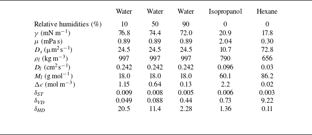
 25∘
 a=1
 ds=10

 ϕ⋆=0.01
 tc≈0.9283
 r(ξ,0)=ξ
 1−ξ
 ϕin(r,t)
 ϕin(r,t)=ϕc
 hin(r,t)

 ϕ⋆
 ϕ⋆=0.01
 tc≈0.9283
 tc−tc0≈2.628×10⁻³
 h0(r,t)
 r(ξ,0)=ξ
 τ0

 ϕ⋆
 ϕ⋆=10−4
 tc≈0.9926
 tc−tc0≈6.432×10⁻⁵
 tc0
 A1
 A2
 r=ξ¯ϕ⋆3/16
 ξ¯/ξ¯i=0,0.1,…,2.0
 ξi(tc)∼ξ¯iϕ⋆3/16

 α
 A
 B
 α→1/4
 A,B→1
 ϕ⋆→0
 ϕ⋆
 α≈0.246,0.239,0.216,0.145
 ϕ⋆=10−4,10−3,10−2,10−1
 ϕ⋆=0.01

 ϕ⋆
 ϕ⋆

 30∘C
 ϕ⋆
 ϕc=0.64
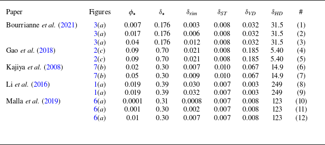
 ϕ⋆
 δ⋆=h⋆/a
 δrim=hmax/a
 ds=22
 Ds=77.6μm2s−1
 Ds=20μm2s−1
 ds=216
 ds=100
 Ds
 ds
 Ds
 #

 wmax
 ϕ⋆
 wmax0
 hmax
 ϕ⋆
 hmax0
 ϕ⋆
 ϕc=0.64


 Open access

