1 Introduction
Dusty plasma is one of the fields of basic research at the present forefront of plasma science. It is one of the forms of complex plasmas containing grains and dust particles (extremely massive charged micro-particulate). The presence of charged dust particles brings about a significant change in the (collective) properties of the plasma medium. There has been much interest in dusty plasmas, because of their importance in the study of space environment research, such as of the rings of Saturn, in cometary tails or in the interstellar medium, see e.g. Horanyi & Mendis (Reference Horanyi and Mendis1986), Goertz (Reference Goertz1989), Mendis & Rosenberg (Reference Mendis and Rosenberg1992), Northrop (Reference Northrop1992). They are also present in industrial processing and laboratory plasmas such as flames and laboratory industrial plasmas (Selwyn Reference Selwyn1993; Hayashi & Tachibana Reference Hayashi and Tachibana1994; Thomas, Morfill & Dammel Reference Thomas, Morfill and Dammel1994). A detailed analysis and discussion of dusty plasmas can be found in Nakamura, Yokota & Shukla (Reference Nakamura, Yokota and Shukla2000), Shukla & Mamun (Reference Shukla and Mamun2002) and Fortov & Morfill (Reference Fortov and Morfill2010).
One of the important acoustic modes in (uniform, unmagnetized, collisionless) plasmas is the ion-acoustic wave (IAW). These waves are longitudinal density perturbations which are produced by oscillations of ions and electrons in the low-frequency mode. Taking into account the presence of dust in this plasma, they may be termed dust ion-acoustic waves (DIAW). The linear and nonlinear aspects of DIAW have been quite well studied and our interest here is due to the nonlinear aspects.
Nonlinear theory for IAW was first considered in Leontovich (Reference Leontovich1966). It has been established that stationary IAW can exist in the form of periodic or localized waves. The physics of nonlinear aspects in plasma (especially in the collective modes in dusty plasmas) has seen significant progress and is one of the leading mainstreams in modern research of plasmas. As is well known, the presence of nonlinearity can lead to a number of interesting localized structures such as solitary waves (solitons), shock fronts, etc. The nonlinear propagation of solitary waves and shock waves occupy an important place in the present-day physics of dusty plasmas. The nonlinear propagations have been widely studied to gain an understanding of the electrostatic disturbances in space plasma environments (Grün, Morfill & Mendis Reference Grün, Morfill and Mendis1984; Goertz Reference Goertz1989) and in laboratory plasma devices (Barkan, D’Angelo & Merlino Reference Barkan, D’Angelo and Merlino1994; Adhikary, Deka & Bailung Reference Adhikary, Deka and Bailung2009). The existence and formation of dust ion-acoustic shocks in dusty plasmas have been studied by many laboratory experiments (Luo & Merlino Reference Luo and Merlino1999; Nakamura, Bailung, & Shukla Reference Nakamura, Bailung and Shukla1999; Luo, D’Angelo & Merlino Reference Luo, D’Angelo and Merlino2000).
Also, from the anomalous dissipation viewpoint, the existence of the dust ion-acoustic shock has been proved analytically (Popel, Yu & Tsytovich Reference Popel, Yu and Tsytovich1996). Linear theory is valid only when the wave amplitude is so small that one may neglect the nonlinearities. However, the dusty plasma is a nonlinear medium and waves of finite amplitude cannot be generally considered independently. Due to a large number of different wave modes which (the unstable modes) can saturate and attain large amplitudes, there are numerous processes leading to different types of nonlinear coherent structures such as shock and solitary waves. The latter are important from both theoretical and experimental points of view and have been studied in the literature, e.g. Kim (Reference Kim1977), Nakamura (Reference Nakamura1987), Bharuthram & Shukla (Reference Bharuthram and Shukla1992), Sheridan (Reference Sheridan1998), Khanna, Brinks & Mould (Reference Khanna, Brinks and Mould2015). The solitons are formed when nonlinear steepening is balanced by dispersion. When the lowest-order nonlinear terms are quadratic, the weakly nonlinear soliton dynamics is governed by the Korteweg–de Vries (KdV) equation. The third-order KdV equation is of the form
 $$\begin{eqnarray}\frac{\partial u}{\partial t}+f(u)\frac{\partial u}{\partial x}+\frac{\partial ^{3}u}{\partial x^{3}}=0,\end{eqnarray}$$
where
 $u=u(x,t)$
is a function of space
 $x$
and the time variable
 $t$
. The nonlinear term
 $f(u)$
appears in many of forms which for
 $f(u)=\pm 6u$
and
 $f(u)=6u^{2}$
, the KdV equation is completely integrable. The case
 $f(u)=6u^{2}$
is known as modified KdV and appears in multi-component plasmas.
As mentioned, a stable soliton solution is obtained by balancing the steepening due to nonlinearity and the dispersion effect of higher-order terms. When the amplitudes of the waves and the dissipation are sufficiently large, nonlinearities can no longer be neglected and can overcome the dispersion effects and this precedence can generate solitons or shock waves. The conventional dissipation is often determined by viscosity, and then the nonlinearity can be described by the KdV–Burgers equation:
 $$\begin{eqnarray}\frac{\partial u}{\partial t}+6u\frac{\partial u}{\partial x}+a\frac{\partial ^{2}u}{\partial x^{2}}+\frac{\partial ^{3}u}{\partial x^{3}}=0,\quad a\neq 0,\end{eqnarray}$$
which admits both rarefactive solitons as well as shocks. The rarefactive dust lattice solitons appear in a collisionless dusty plasma with
 $a=0$
.
It is important to emphasize the difference between the current dusty plasma (containing electrons, positive ion and negatively charged dust grains) and a multi-component plasma (containing electrons, positively and negatively charged ions). The remarkable difference is the much higher amount of charge residing in the dust grains in the dusty plasma. Such a difference causes different dynamics for these two type of plasmas, including shocks and solitary waves. For example, the formation and excitation of nonlinear solitary waves in inhomogeneous magnetized plasmas having negative ions have been studied in Malik & Kawata (Reference Malik and Kawata2007), Malik & Stroth (Reference Malik and Stroth2008), Singh & Malik (Reference Singh and Malik2008) and the nonlinear solitary waves in plasmas including (impurity) dust particles in (Kumar & Malik Reference Kumar and Malik2011; Kumar, Malik & Singh Reference Kumar, Malik and Singh2012; Malik & Malik Reference Malik and Malik2014). Also, the difference is important from another aspect, that is, dust particles differ from negative ions in that their charge is not a fixed quantity and therefore, this can also cause different dynamics. For instance, the reflection and transmission of an ion-acoustic soliton in a dusty plasma with variably charged dust has been studied in Malik, Tomar & Dahiya (Reference Malik, Tomar and Dahiya2014).
The other successful approach for the study of nonlinear effects described by (1.1) and (1.2) is the Sagdeev potential (SP) method (also called the quasi-potential method). This method is a very convenient approach to the study of solitons of arbitrary amplitude. One can derive all of the one soliton solutions with perturbation methods and compare them with the exact results obtained by the quasi-potential method.
In this work, we consider the collective motion of the negatively charged dust particles in a background of hot electrons and ions in thermodynamic equilibrium in a dusty plasma. The dusty plasma is assumed to be unmagnetized and collisionless and it is composed of three components, namely negatively charged dust grains, hot electrons and ions. By identifying the number density and distribution function for each of the constituent particles of the dusty plasma, the SP is determined for our model and we employ it to compute the width of the solitary waveFootnote
1
for the ion-acoustic wave propagated in dusty plasma. The collective dynamics is governed by the Vlasov–Ampere–Gauss system of equations and we focus on (the travelling wave) far-field solutions which are asymptotic solutions to the initial value conditions (Turski, Atamaniuk & Uchowski Reference Turski, Atamaniuk and Uchowski1999). The dusty plasma has three important parameters which have an important role in our discussion and analysis. The parameters include Mach number
 $M$
, ion–electron temperature ratio
 $R$
and the dust–ion charge ratio
 $S$
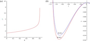
whose values are allowed in certain ranges. Our main purpose is to find the relationship between the width of the solitary wave and the values of the plasma parameters. In the other words, we want to know how the width changes when we change any of the parameters. Because of the complexity of the relevant equations, we cannot obtain an explicit function of the parameters and we have to use a numerical method to illustrate the width changes versus each parameter. Due to the lack of an explicit function, a graphical solution can help us to understand how to change the width function.
Our analysis is based on the analogy between SP and the one-dimensional (say
 $x$
) potential energy for a real particle moving in conservative field. For such a particle, the energy conservation theorem can be written as
 $$\begin{eqnarray}\frac{1}{2}m\left(\frac{\text{d}x}{\text{d}t}\right)^{2}+U(x)=E=\text{constant},\end{eqnarray}$$
where
 $U(x)$
is the potential energy. If the particle is subjected to small oscillations around an equilibrium point
 $x_{m}$
, the angular frequency of the small oscillations is given by
 $$\begin{eqnarray}{\it\omega}^{2}=\frac{1}{m}\left.\frac{\text{d}^{2}U(x)}{\text{d}x^{2}}\right|_{x=x_{m}}.\end{eqnarray}$$
On the other hand, for the plasmas in this work, the SP (say
 $V({\it\phi})$
) satisfies the following energy conservation law
 $$\begin{eqnarray}\frac{1}{2}\left(\frac{\text{d}{\it\phi}}{\text{d}{\it\xi}}\right)^{2}+V({\it\phi})=0,\end{eqnarray}$$
where
 ${\it\phi}$
is electrostatic potential. In view of analogy considerations, (1.3) and (1.5) are analogues and hence the former can be regarded as energy condition for a (pseudo) particle of unit mass (
 $m=1$
) with
 $E=0$
. According to this analogy, the potential
 ${\it\phi}$
plays the role of position and the coordinate position
 ${\it\xi}$
plays the role of time. Therefore, the plasma counterpart of (1.4), can be written as
 $$\begin{eqnarray}k_{s}^{2}=\left.\frac{\text{d}^{2}V({\it\phi})}{\text{d}{\it\phi}^{2}}\right|_{{\it\phi}={\it\varphi}_{m}},\end{eqnarray}$$
where the analogue of
 ${\it\omega}$
(in (1.4)) is denoted by
 $k_{s}$
. It is easy to check that
 $k_{s}$
has the dimensions of inverse length.
For a given potential energy,
 $U=U(x)$
, even in cases where the equation of motion cannot easily be integrated or the resulting equation is solved to give an explicit solution for
 $x(t)$
, a lot of useful information about the motion can be obtained from the potential curve, that is, the graph of
 $U(x)$
versus
 $x$
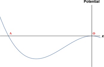
. It is interesting to note that the general character of the motion, as inferred from the energy diagram, would be the same for any potential curve, including the SP one. According to this, we can give the following description of (pseudo) particle motion in an arbitrary potential well with the shape illustrated in figure 1.Footnote
2
A potential curve including a well.

The (pseudo) particle (of zero energy) enters the well from the right (point O) and will go to the left-hand side of the well. Because of energy conservation, at the first point at which the potential vanishes (point A), it must stop and return to the entrance point. Thus, it makes a single transition between two points and this is nothing other than a soliton, which is propagated in the medium as a potential disturbance. However, when the system undergoes small energy dissipations, the (pseudo) particle will never return to the entrance point and is trapped inside the well and oscillates about the equilibrium point
 ${\it\varphi}_{m}$
. In what follows below and using this mechanical analogy, we obtain an equation to calculate the soliton width.
In the oscillation motion of a real particle with angular frequency
 ${\it\omega}$
, the motion period is given by:
 $$\begin{eqnarray}\displaystyle & & \displaystyle T=\text{a time interval corresponding to one complete temporal}\nonumber\\ \displaystyle & & \displaystyle \qquad \text{oscillation of a real particle in the well}=2{\rm\pi}/{\it\omega},\end{eqnarray}$$
which, using (1.4), gives
 $$\begin{eqnarray}T=2{\rm\pi}/\sqrt{U^{\prime \prime }(x_{m})/m}.\end{eqnarray}$$
On the other hand, owing to the above definition of a soliton, that is, one complete oscillation of a pseudo-particle in the SP well, we can write
 $$\begin{eqnarray}\displaystyle & & \displaystyle {\it\lambda}_{s}=\text{a distance interval corresponding to one complete spatial oscillation}\nonumber\\ \displaystyle & & \displaystyle \quad \quad \text{of a pseudo-particle in the well}=2{\rm\pi}/k_{s},\end{eqnarray}$$
which, using (1.6), gives
 $$\begin{eqnarray}{\it\lambda}_{s}=2{\rm\pi}/\sqrt{V^{\prime \prime }({\it\varphi}_{m})}.\end{eqnarray}$$
Since the above definition for
 ${\it\lambda}_{s}$
is the definition of soliton width, thus (1.10) is the basic formula for our computation in the work. This is the reason why the width is given by a second derivative.
As we will see, because of the complication of the function (1.10), it cannot be generally expressed in an explicit form (in terms of plasma parameters). Hence, it is not possible to have any information about its overall behaviour. Therefore, to illustrate the graph of the width function, we have to use numerical plotting (by computer algebra) which largely contributes to our understanding of the behaviour of the function. One such analytical treatment discussed above has been used to compute and illustrate the width of the shock wave propagated in a pair plasma (Malakolkalami & Mohammadi Reference Malakolkalami and Mohammadi2014).
The work is organized as follows:
In the next section, the basic equations and the model are introduced. In § 3, the SP method is employed to compute the soliton width (function) and its corresponding graphs are presented. The conclusions and remarks are given in the last section.
2 Basic equations and the model
We investigate the nonlinear characteristics of DIAW which propagate as solitons with negative electrostatic potential. Let us consider a three-component unmagnetized dusty plasma (dust (d)–electron (e)–ion (i)). The dynamics of one-dimensional ion-acoustic oscillations is given by the Vlasov–Ampere–Gauss system of equations (Turski et al. Reference Turski, Atamaniuk and Uchowski1999; Turski, Atamaniuk & Turska Reference Turski, Atamaniuk and Turska2003):
 $$\begin{eqnarray}\displaystyle & \displaystyle \left(\partial _{t}+u\partial _{x}+\frac{q_{{\it\alpha}}}{m_{{\it\alpha}}}E(x,t)\partial _{u}\right)f_{{\it\alpha}}(u,x,t)=0, & \displaystyle\end{eqnarray}$$
 $$\begin{eqnarray}\displaystyle & \displaystyle {\it\varepsilon}_{0}\partial _{t}E+\mathop{\sum }_{{\it\alpha}}q_{{\it\alpha}}\int _{-\infty }^{+\infty }uf_{{\it\alpha}}\,\text{d}u=0, & \displaystyle\end{eqnarray}$$
 $$\begin{eqnarray}\displaystyle & \displaystyle {\it\varepsilon}_{0}\partial _{x}E+\mathop{\sum }_{{\it\alpha}}q_{{\it\alpha}}\int _{-\infty }^{+\infty }f_{{\it\alpha}}\,\text{d}u=0, & \displaystyle\end{eqnarray}$$
 $f_{{\it\alpha}},q_{{\it\alpha}}$
and
 $E(x,t)$
are the distribution function, electric charge of species
 ${\it\alpha}$
and electric field, respectively. The number densities of plasma components in equilibrium state are
 $N_{0{\it\alpha}(=d,e,i)}$
and ion temperature and electron temperature are denoted by,
 $T_{i}$
and
 $T_{e}$
, respectively. The total charge neutrality condition (
 $N_{0i}=ZN_{0d}+N_{0e}$
) is to be assumed where
 $Z$
is the number of electrons residing on the dust grain surface at equilibrium, that is
 $q_{d}=-Ze$
.
Assuming the Dirac delta equilibrium distribution for a cold plasma species (dust grains) and (square) pulse equilibrium distribution (Heaviside function) for hot plasma species (ions and electrons), then it can be shown that a stationary far-field solution exists and the corresponding particle number densities take the following forms (Turski et al. Reference Turski, Atamaniuk and Turska2003):
 $$\begin{eqnarray}\displaystyle & \displaystyle n_{c}=\frac{N_{0c}}{\sqrt{1-{\displaystyle \frac{2q_{c}{\it\phi}}{m_{c}U^{2}}}}}, & \displaystyle\end{eqnarray}$$
 $$\begin{eqnarray}\displaystyle & \displaystyle n_{h}=N_{0h}\frac{v_{h}+U}{2v_{h}}\sqrt{1-\frac{2q_{h}{\it\phi}}{m_{h}(v_{h}+U)^{2}}}+N_{0h}\frac{v_{h}-U}{2v_{h}}\sqrt{1-{\displaystyle \frac{2q_{h}{\it\phi}}{m_{h}(v_{h}-U)^{2}}}}, & \displaystyle\end{eqnarray}$$
 $U$
and
 $v_{h}$
are the phase velocity of the wave and thermal velocity, respectively and the index c (h) stands for cold (hot) species. Moreover, we assume that the localized structures (solitons) move at velocities of an order which should be less than the electron and ion thermal velocity, that is
 $U/v_{h}\ll 1$
. Under this assumption, it is easy to show that, up to the first power in binomial expansion, the right-hand side of (2.5) is approximated by Turski et al. (Reference Turski, Atamaniuk and Uchowski1999):
 $$\begin{eqnarray}n_{h}\approx N_{0h}\sqrt{1-\frac{2q_{h}{\it\phi}}{m_{h}v_{h}^{2}}}.\end{eqnarray}$$
Given the above number densities (2.4) and (2.6), one can calculate the SP.
2.1 Sagdeev potential
Assuming an stationary solution, to study the evolution of the waves, we transform the set of equations (2.1)–(2.3) to a stationary frame moving with the phase velocity of the wave
 $U$
. Therefore, by making use of coordinate transformation
 ${\it\xi}=x-Ut$
(normalized by the Debye length of the ion plasma
 ${\it\lambda}_{Di}=\sqrt{T_{i}/4{\rm\pi}N_{0i}e^{2}}$
) and taking the normalized potential
 $y({\it\xi})=(e{\it\phi}({\it\xi}))/(m_{i}v_{i}^{2})$
, the SP can be written Turski et al. (Reference Turski, Atamaniuk and Uchowski1999, Reference Turski, Atamaniuk and Turska2003):
 $$\begin{eqnarray}\displaystyle V(y) & = & \displaystyle \mathop{\sum }_{{\it\alpha}}V_{{\it\alpha}}(y)=V_{d}(y)+V_{e}(y)+V_{i}(y)=SM^{2}\left(1-\sqrt{1+\frac{2y}{M^{2}}}\right)\nonumber\\ \displaystyle & & \displaystyle +\,\frac{1}{3}(1-(1-2y)^{3/2})+\frac{1-S}{3R}(1-(1+2Ry)^{3/2}),\quad y<0,\end{eqnarray}$$
where the three important parameters
 $M$
,
 $R$
and
 $S$
are defined by
 $$\begin{eqnarray}M=\text{Mach number}=U/c_{s},\end{eqnarray}$$
 $$\begin{eqnarray}R=\text{ion{-}electron temperature ratio}=T_{i}/T_{e},\end{eqnarray}$$
 $$\begin{eqnarray}S=\text{dust{-}ion charge ratio}=ZN_{0d}/N_{0i},\end{eqnarray}$$
where
 $c_{s}=v_{i}\left(Zm_{i}/m_{d}\right)^{1/2}$
is the dust–ion sound speed. The range of the parameters can easily be fixed because we have
 $$\begin{eqnarray}c_{s}<U,\quad T_{i}<T_{e}\quad \text{and}\quad ZN_{0d}<N_{0i},\end{eqnarray}$$
and so it is easy to check that (Turski et al. Reference Turski, Atamaniuk and Uchowski1999, Reference Turski, Atamaniuk and Turska2003):
 $$\begin{eqnarray}M>1\quad \text{and}\quad 0<S,R<1.\end{eqnarray}$$
Since, we are looking for soliton solutions, it is important to choose the appropriate values of the parameters in their allowed ranges. This means that any choice of the parameters (even in their allowed ranges) does not necessarily lead to a soliton solution. The necessary conditions for the existence of solitary waves are:
 $$\begin{eqnarray}V(0)=V^{\prime }(0)=0\quad \text{and}\quad V^{\prime \prime }(0)<0,\end{eqnarray}$$
of course, the form of the SP (2.7) would determine whether soliton solutions may exist or not. In our model, only negative potential solitons (rarefactive solitons) are admissible due to the presence of negatively charged dust grains. That is, the well structures of the SP allow only dust ion-acoustic solitons with negative potential. In addition to the conditions (2.13), the following sufficient condition also must be satisfied: there should be an electrostatic potential
 ${\it\phi}_{m}$
such that
 $V({\it\phi})<0$
for
 ${\it\phi}_{m}<{\it\phi}<0$
, and
 $V({\it\phi})>0$
for
 ${\it\phi}<{\it\phi}_{m}$
and also
 $V({\it\phi}_{m})=0$
.Footnote
3
In preparation for the next section, we calculate the following derivatives from (2.7):
 $$\begin{eqnarray}V^{\prime }(y)=-\frac{S}{\sqrt{1+{\displaystyle \frac{2y}{M^{2}}}}}+\sqrt{1-2y}-(1-S)\sqrt{1+2Ry},\end{eqnarray}$$
 $$\begin{eqnarray}V^{\prime \prime }(y)=\frac{S/M^{2}}{\left(1+{\displaystyle \frac{2y}{M^{2}}}\right)^{3/2}}-\frac{1}{\sqrt{1-2y}}-{\displaystyle \frac{(1-S)R}{\sqrt{1+2Ry}}}.\end{eqnarray}$$
At the end of this section, two points should be noted:
-
(1) Since, in the low-frequency mode, the behaviour of a dusty plasma is very similar to that of a plasma consisting of negative ions, many results from the theory of negative-ion plasmas can be adapted to dusty plasmas (Rao et al. Reference Rao, Shukla and Yu1990).
-
(2) Because of the large mass of the dust grains, namely
 $m_{d}\gg m_{i}\gg m_{e}$
, the ion plasma frequency is much larger than the dust plasma frequency and therefore, the dynamics may be neglected from the dust inertia.

3 The soliton width as a function of the plasma parameters
To compute the width of the solitary wave, we return now to the mechanical analogy discussed in § 1. It is an analogy between the oscillation of a pseudo-particle in a pseudo-potential well and the oscillation of a real particle in a potential well. As explained, we are interested in the oscillatory motion of a particle around an equilibrium point for which the angular frequency of the small oscillations is given by (1.4). Therefore, we can make an analogous replacement in the case of a dusty plasma according to the following in (1.4):
 $$\begin{eqnarray}{\it\omega}\rightarrow k_{s},\quad U\rightarrow V,\quad x\rightarrow y\quad \text{and}\quad m\rightarrow 1\end{eqnarray}$$
which gives
 $$\begin{eqnarray}k_{s}^{2}=\left.V^{\prime \prime }(y_{m})=\frac{\text{d}^{2}V(y)}{\text{d}y^{2}}\right|_{y=y_{m}},\end{eqnarray}$$
and hence the width function becomes
 $$\begin{eqnarray}{\it\lambda}_{s}=2{\rm\pi}/k_{s}=\frac{2{\rm\pi}}{\sqrt{V^{\prime \prime }(y_{m})}}.\end{eqnarray}$$
We note that the equilibrium point
 $y_{m}$
is determined by a vanishing first derivative (2.14), that is
 $$\begin{eqnarray}V^{\prime }(y_{m})=-\frac{S}{\sqrt{1+{\displaystyle \frac{2y_{m}}{M^{2}}}}}+\sqrt{1-2y_{m}}-(1-S)\sqrt{1+2Ry_{m}}=0,\end{eqnarray}$$
this equation is an algebraic one for which there is no formula to find its exact solution, that is, it cannot be solved for
 $y_{m}$
in terms of the parameters
 $M$
,
 $R$
and
 $S$
. In other words, (3.4) defines an implicit function
 $y_{m}$
and hence it does not allow us to have any information of the behaviour of the function (3.3). Although an explicit form of the defined function is unknown, the graph of function (3.3) can be illustrated by numerical plotting and as we will see, (equation (3.3)) provides useful information about its behaviour.
To investigate and illustrate the dependence of the width function (3.3) on each parameter, let us keep two of the parameters (say
 $R$
and
 $S$
) fixed and consider the function of one parameter
 ${\it\lambda}_{s}=f(M)$
. This procedure is carried out for all parameters in three following case:
(I)
 ${\it\lambda}_{s}$
as a function of
 $M$
:
In this case, for any allowed fixed values of parameters
 $S$
and
 $R$
, the soliton width (3.3) is a function of
 $M$
. We begin with the case
 $S=1$
which is independent on the ion–electron temperature ratio
 $R$
(the electron number density vanishes). Indeed, this case is the only exact one which we can obtain in a closed form for the width function (3.3). From a physics point of view, this is a two-component (dusty) plasma, something like a pair plasma in which the electrons carry a charge greater than
 $-e$
.
Substituting
 $S=1$
into (3.4) and solving for
 $y_{m}$
, we obtain
 $$\begin{eqnarray}y_{m}=\frac{1-M^{2}}{2}.\end{eqnarray}$$
Remember that if
 $M>1$
then
 $y_{m}<0$
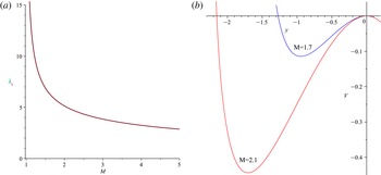
. The graph of the SP (2.7) is illustrated in figure 2(b) for
 $S=1$
and the two values of
 $M$
. Substituting (3.5) into the right-hand side of the second derivative (2.15) gives
 $$\begin{eqnarray}\displaystyle k_{s}^{2}={\it\lambda}_{s}(M)=M-\frac{1}{M}=\frac{M^{2}-1}{M}, & & \displaystyle\end{eqnarray}$$
and finally, the width function (3.3) takes the form
 $$\begin{eqnarray}\displaystyle {\it\lambda}_{s}={\it\lambda}_{s}(M)=2{\rm\pi}\sqrt{\frac{M}{M^{2}-1}}. & & \displaystyle\end{eqnarray}$$
This function is plotted in figure 2(a) and represents a decreasing monotonic function over the interval
 $(1,\infty )$
. As the figure shows, the function drops off rapidly up to
 $M\approx 3$
. The form of the graph may be explained as follows:
The value of
 ${\it\lambda}_{s}$
is the length of a complete oscillation (of the pseudo-particle) in the potential well and the narrower wells correspond to a greater Mach number (figure 2
b), thus the generated solitons corresponding to the greater
 $M$
have lower width.
(a) Plot of the width versus
 $M$
and (b) SP curves versus
 $y$
for
 $S=1$
and two different values of
 $M$
.

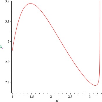
Plot of the width versus
 $M$
for
 $S=0.8$
and
 $R=0.1$
.

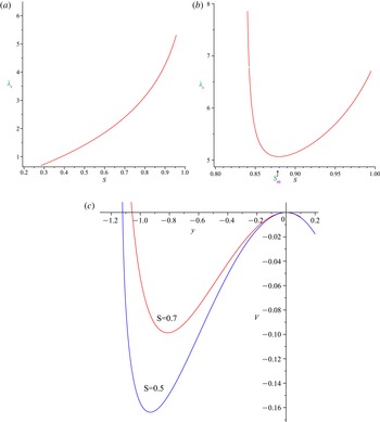
Plot of the width versus
 $S$
for the values, (a)
 $M=1.5$
,
 $R=0.03$
and (b)
 $M=1.5$
,
 $R=0.6$
– (c) SP curves versus
 $y$
for the values
 $M=1.5$
and
 $R=0.01$
.

(a) Plot of the width versus
 $R$
, for the values
 $M=1.5$
and
 $S=0.6$
(b) SP curves versus
 $y$
for the values
 $M=1.5$
and
 $S=0.6$
.

It should be noted that the latter statement is true not only for two potential wells corresponding to different values of Mach numbers, but also for two different values of the other parameters
 $S$
or
 $R$
. This means that if we consider two potential wells corresponding to two different values for one of the parameters
 $M$
,
 $S$
and
 $R$
, then the narrower (wider) well generates the soliton of smaller (larger) width. This is important in order to understand the variations of the width function.
As mentioned, the previous case (
 $S=1$
) was independent of the temperature ratio parameter, but for any other value (i.e.
 $S\neq 1$
), the value of the parameter
 $R$
should be determined and fixed. In this case, the width function cannot be expressed in a closed form and therefore, the graphical solution may be obtained only by a numerical method. For the fixed values
 $S=0.8$
and
 $R=0.1$
, the numerical graph is illustrated in figure 3. The figure shows that the graph has local and global extremum, unlike the graph corresponding to the two-component plasma (
 $S=1$
) which demonstrates a monotonic decreasing function (figure 2
a). Indeed, figure 3 indicates that
 ${\it\lambda}_{s}$
increases over the (approximate) interval
 $1<M<1.5$
, and then decreases over
 $1.5<M<3.1$
, after which a rapid increase (not to infinity) takes place along the curve over a comparatively small increase in the Mach number.
(II)
 ${\it\lambda}_{s}$
as a function of
 $S$
:
For any allowed fixed values of
 $M$
and
 $R$
, the width is a function over the interval
 $0<S<1$
. A numeric graphical representation of the function (3.3) is illustrated in figure 4(a) for
 $R=0.03,M=1.5$
. The graph represents a monotonic increasing function of
 $S$
. In fact, this case may be considered as a low temperature limit (
 $R\ll 1$
) and figure 4(a) shows the character of this case qualitatively. There is an absolute minimum point (here
 $S=S_{m}\approx 0.28$
) for which
 ${\it\lambda}_{s}\approx 0$
and there is an absolute maximum point (here
 $S\approx 1$
) for the width function (
 ${\it\lambda}_{s}\approx 5.5$
).
The figure 4(b) is the graph of the width function for
 $R=0.6,M=1.5$
and it may be considered a as high temperature limit. There is an absolute minimum point (here
 $S=S_{m}\approx 0.88$
) for which
 ${\it\lambda}_{s}\neq 0$
and also an absolute maximum point (here
 $S\approx 1$
) for the width function (
 ${\it\lambda}_{s}\approx 6.75$
).
It should be noted that the decreasing part of the graph in figure 4(b) (approximately
 $0<S<0.88$
) corresponds to the motion of the pseudo-particle in a region for which a soliton solution does not exist and thus, the decreasing part of the graph is not admissible. More precisely, the potential wells cannot be formed for any allowed values of
 $0<S<1$
but they can be formed from a certain point onwards (here
 $S=S_{m}\approx 0.88$
).
Therefore, in the both temperature limits, there are soliton solutions and the width
 ${\it\lambda}_{s}$
is a monotonic increasing function of
 $S$
, but the allowable range (
 $0<S<1$
) is reduced.
(III)
 ${\it\lambda}_{s}$
as a function of
 $R$
:
By fixing the values of parameters
 $M$
and
 $S$
, we can find the soliton width as a function of
 $R$
. For
 $M=1.5$
and
 $S=0.6$
, a numerical plot of the function is presented in figure 5(a). The figure illustrates the graph of the width function over the interval
 $0<R<0.53$
. Out of the interval, there is no soliton solution unless
 $S\rightarrow 1$
, because, as previously mentioned, the case
 $S=1$
is independent of the temperature ratio
 $R$
. In other words, for any allowable choice of parameters
 $M$
and
 $S$
, the temperature ratio parameter
 $R$
cannot take any value in its allowable range, that is
 $0<R<1$
. This is the same situation we encountered in the previous case II in which there is not a soliton solution for any (arbitrary) value of
 $S$
in its allowable range. We note that, figure 5(a) illustrates an increasing monotonic function over the interval
 $0<R<0.53$
where it represents a slowly increasing function over a large part of the interval, and a rapidly increasing one (not infinity) over the small rest interval. The upward slope of the width graph can be explained as follows:
Based on figure 5(b), the potential well corresponding to the larger value (
 $R=0.2$
) is wider than the smaller one (
 $R=0.1$
) and hence,
 ${\it\lambda}_{s}$
is increased.
In the end of this section, it is necessary to say that our ability to plot the graph of the width function
 ${\it\lambda}_{s}$
(as continues function) is because of the analytical form of the SP (2.7). Indeed, the method presented in this work can be used to compute and plot a graph of the soliton width for any SP of analytic form. When the SP has no analytic form, there is no such possibility, although we can still calculate numerically
 ${\it\lambda}_{s}$
at each allowable equilibrium point. This is based on estimation of the equilibrium point and substitution of the estimated value in the second derivative. In this case we have a (discrete) point diagram instead of a continues curve. One such computation has been represented in Malakolkalami & Mohammadi (Reference Malakolkalami and Mohammadi2012) for an electron–positron plasma including stationary ions in the background.Footnote
4
3.1 Amplitude of the solitary wave
In this subsection, we give a brief discussion of the soliton amplitude and how it depends on the dusty plasma parameters.
The shock amplitude
 ${\it\phi}_{m}$
may be obtained by solving the equation:
 $$\begin{eqnarray}V(y)=SM^{2}\left(1-\sqrt{1+\frac{2y}{M^{2}}}\right)+\frac{1}{3}(1-(1-2y)^{3/2})+\frac{1-S}{3R}(1-(1+2Ry)^{3/2})=0,\end{eqnarray}$$
with
 $y=e{\it\phi}_{m}/mv_{i}^{2}$
. Equation (3.8) cannot be easily solved for
 $y$
but fortunately, as we know,
 ${\it\phi}_{m}$
is determined by the point of intersection (except
 $y=0$
) of the SP curve and the
 $y$
axis, hence, it is possible to provide a quantitative description of the amplitude by referring to the SP curves. From this we may conclude that:
-
(A) According to figure 2(b), the amplitude increases with increasing Mach number.
-
(B) According to figure 4(c), the amplitude decreases with increasing dust–ion charge ratio, that is, either increasing the elementary negative charge on the dust grains or the number density of the dust grains.
-
(C) According to figure 5(b), the amplitude increases with increasing ion–electron temperature ratio.
We note that the results A and B are contrary to the width change which decreases with increasing Mach number and result C is the same as that of the width change.
3.2 Concerns and applications
As mentioned in the introduction, the study of a dusty plasma and its physical properties has an important place in plasma research. Dusty plasmas are encountered in various branches of research including industrial processing plasmas, space plasmas, the mesosphere of the Earth and specifically designed laboratory experiments. Also, a variety of wave phenomena in dusty plasmas have been described. One of the important waves in dusty plasmas are electrostatic modes among which are the ion-acoustics waves. These waves can propagate both linearly and nonlinearly in a dusty plasma. The most significant nonlinear phenomena may be shock and solitary wave propagation and associated physical quantities such as the width and the amplitude. Since dust is present in space and astrophysical environments, one of the main research fields of plasma astrophysics may be related to dusty and grain plasma and the propagation of ion-acoustic solitons and shocks Peratt (Reference Peratt2015). Examples of dusty plasmas in space plasma include comets, planetary rings, exposed dusty surfaces and the zodiacal dust cloud. Moreover, dust particles in interstellar space attract much attention in relation to the planetary rings (Shukla & Mamun Reference Shukla and Mamun2002).
From this point of view, the authors do believe that the subject of the manuscript may have some relevance. Specifically, the dusty plasma model discussed here has astrophysical and solar system applications and the acoustic modes have some relevance to low-frequency noise in the F-ring of Saturn (Turski et al. Reference Turski, Atamaniuk and Turska2003).
4 Conclusions
In this manuscript we have considered an unmagnetized, collisionless dusty plasma containing three components (dust grain–ion–electron). Given the propagation of an ion-acoustic solitary wave, we have attempted to compute the width of the solitary wave as a function of the plasma parameters. The parameters are the Mach number
 $M$
, ion–electron temperature ratio
 $R$
and dust–ion charge ratio
 $S$
. The allowable range of parameters are determined and fixed by their definitions.
The Vlasov–Ampre–Gauss system of equations describes the nonlinear dynamics of the model and the SP method is employed to obtain an equation describing the width function. Because of the complexity of the relations which are given in the implicit representation, it is not possible to obtain a function in an explicit form and thus we have to use a numerical method to illustrate the graph of the width function. To display the function dependence on each parameter, the three following cases are distinguished:
(I) The soliton width is a function of the Mach number:
For any allowed fixed values of parameters
 $R$
and
 $S$
, the soliton width becomes a function of the Mach number. For the particularly simple case
 $S=1$
and
 $R=$
arbitrary, the graph of the width function represents a rapidly monotonic decreasing function. In this case, the electrons are not present and in fact it is a two-component plasma (dust–ion), something like a pair plasma. The presence of electrons changes the monotonic nature of the width function. For example, by choosing the values
 $S=0.8,R=0.1$
, we have the graph of ascending and descending parts, as illustrated in figure 2.
(II) The soliton width is a function of the dust–ion charge ratio:
We consider
 $M=1.5$
and two different values (
 $R=0.03,0.6$
). The latter values can be regarded as low (
 $R\ll 1$
) and high (
 $R\rightarrow 1$
) temperature limits, respectively. There is no qualitative difference between the plots corresponding to (
 $R\ll 1$
) and (
 $R\rightarrow 1$
), because in the both limits, the width of the solitary waves are a monotonic increasing function. However, in the low limit
 $R=0.03$
, there is a (non-vanishing minimum) value of
 $S$
for which the soliton width vanishes, but in the high limit
 $R=0.6$
, there is a minimum value
 $S_{m}\neq 0$
for which
 ${\it\lambda}_{s}$
has a non-zero absolute minimum value. Indeed, soliton solutions can exist for
 $S_{m}<S<1$
where
 $S_{m}$
depends on the chosen values for
 $M$
and
 $R$
.
(III) The soliton width is a function of the ion–electron temperature ratio:
With the fixed values
 $M=1.5$
and
 $S=0.6$
, the width is a monotonic increasing function of
 $R$
. In this case, there is a non-zero value for the width function at
 $R=0$
, (contrary to the previous case in which there is no soliton solution for
 $S=0$
). In other words, when the ion temperature is much smaller than the electron temperature, the solitary wave can be propagated in the plasma ambient. This is equivalent to saying that a complete potential well can be formed for
 $0\leqslant R<R_{m}<1$
where
 $R_{m}$
depends on the chosen values for
 $M$
and
 $S$
.